Sensitivity Analysis Method for Spectral Band Adjustment between Hyperspectral Sensors: A Case Study Using the CLARREO Pathfinder and HISUI


1
Department of Information Science and Technology, Aichi Prefectural University, 1522-3 Ibaragabasama, Nagaute, Aichi 480-1198, Japan
2
The Institute of Geology and Geoinformation, National Institute of Advanced Industrial Science and Technology (AIST), Central 7, 1-1-1 Higashi, Tsukuba, Ibaraki 305-8567, Japan
Remote Sens. 2019, 11(11), 1367; https://0-doi-org.brum.beds.ac.uk/10.3390/rs11111367
Submission received: 5 May 2019
/
Revised: 30 May 2019
/
Accepted: 5 June 2019
/
Published: 6 June 2019
(This article belongs to the Special Issue Calibration/Validation of Hyperspectral Imagery)
Abstract
:The International Space Station has become the platform for deploying hyperspectral sensors covering the solar reflective spectral range for earth observation. Intercalibration of hyperspectral sensors plays a crucial role in evaluating/improving radiometric consistency. When intercalibrating between hyperspectral sensors, spectral band adjustment is required to mitigate the effects of differences between the relative spectral responses (RSRs) of the sensors. Errors in spectral parameters used in spectral band adjustment are propagated through to the adjustment results. The present study analytically approximated the uncertainty in the spectral band adjustment for evaluating the relative contributions of uncertainties in parameters associated with the exo-atmosphere, atmosphere, and surface to the total uncertainty. Numerical simulations using the derived equations were conducted to perform a sensitivity analysis for the case of the spectral band adjustment between the Climate Absolute Radiance and Refractivity Observatory (CLARREO) Pathfinder (CPF) and the Hyperspectral Imager Suite (HISUI). The results show that the effects of errors in the solar irradiance were greater than those of other sources of error, indicating that accurate estimates of atmospheric reflectances and tranismittances are not needed for spectral band adjustment between CPF and HISUI in the atmospheric windows. The accuracy of the analytical approximation was also evaluated in the simulations. The framework of the sensitivity analysis is applicable to other pairs of hyperspectral sensors.
1. Introduction
The International Space Station (ISS) has become the platform for deploying hyperspectral sensors covering the solar reflective spectral range for earth observation [1]. Currently, the German Aerospace Center (DLR) Earth Sensing Imaging Spectrometer (DESIS) [2] on the ISS makes measurements over the spectral range 400–1000 nm. Hyperspectral sensors will be placed on the ISS, including the Hyperspectral Imager Suite (HISUI) [3], the Earth Surface Mineral Dust Source Investigation (EMIT) [4], and the Climate Absolute Radiance and Refractivity Observatory (CLARREO) Pathfinder (CPF) [5]. Radiometric intercalibration of these sensors plays a crucial role in evaluating radiometric consistency across sensors (e.g., CPF and HISUI [6] and HISUI and DESIS [7]), thereby allowing multiple sensors to be tied onto a common radiometric scale for interoperability and synergistic applications [8,9].
A key objective of the CPF is to use it as a reference for the intercalibration of the earth observation sensors in orbit [10,11,12]. The broadband radiometric accuracy of the CPF is <0.5% and the spectral accuracy is <1% [5]. Intercalibration using the CPF is especially important for multispectral sensors observing parameters necessary for climate studies (e.g., the Visible Infrared Imaging Radiometer Suite (VIIRS) on board the Suomi-National Polar-Orbiting Partnership (NPP) and Joint Polar Satellite System (JPSS) satellites). The CPF would therefore be beneficial as a reference for intercalibration of hyperspectral sensors on board the ISS.
The accuracy of the intercalibration of hyperspectral sensors is influenced by several sources of error, including differences between their relative spectral response (RSR), differences in sun target sensor viewing geometry, uncertainties in radiometric and spectral calibration, potential RSR shifts of sensors, differences in instrument sensitivity to polarized light [13], and relative geolocation errors. Differences in sun target sensor viewing geometry are expected to have relatively small effects when the sensors are mounted on a single platform such as the ISS.
Differences in RSR between sensors give rise to systematic errors in the intercalibration. Mitigating the effects of differences in RSR between sensors requires spectral conversion using a technique called spectral band adjustment, which produces coefficients called spectral band adjustment factors (SBAFs) [14]. SBAFs are often derived from hyperspectral sensors such as the Earth Observing (EO)-1 Hyperion and are successfully used to cross-calibrate satellite sensors (e.g., [15]); however, SBAFs may include errors due to band-to-band calibration inconsistencies [16,17]. SBAFs obtained using the Scanning Imaging Absorption spectrometer for the Atmospheric CHartographY (SCIAMACHY) are also used for spectral band adjustment. This instrument provides reasonable and accurate spectral band adjustment results [9]. The nadir footprint size of the SCIAMACHY product used to derive SBAFs can be extensive (e.g., about 30 km by 240 km [18]) relative to the footprint size of the target sensors.
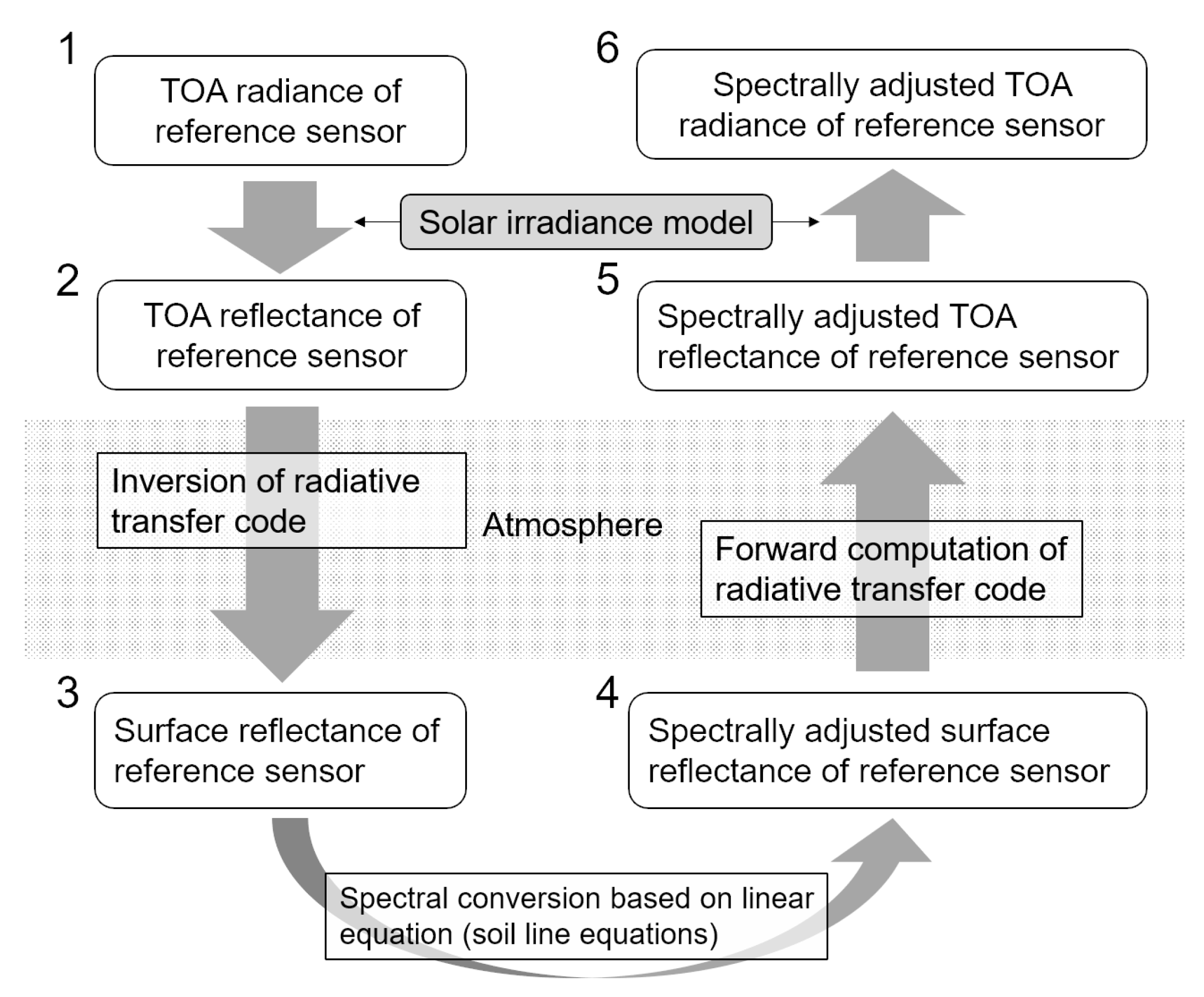
Another approach to spectral band adjustment involves using a model-based spectral band adjustment, in which measurements made using a reference sensor are spectrally converted to those of a spectrally matching band of a destination sensor using an atmospheric radiative transfer code and a linear equation describing the relationships between surface reflectances, as shown in Figure 1. The units of the measurements are those of reflectance or radiance. When the primary signals of reference and destination sensors are calibrated in reflectance units; one should follow Steps 2–5 in Figure 1 (reflectance-to-reflectance conversion). The model-based spectral band adjustment does not require hyperspectral data from satellites, although it does require in-situ measurements of hyperspectral reflectances (e.g., at 1 nm intervals) on surfaces to derive the linear equation [19]. Nevertheless, this approach has been successfully applied to spectral band adjustment in intercalibration studies [19,20,21,22]. In the following sections, the model-based spectral band adjustment is referred to as spectral band adjustment for simplicity.
The overall uncertainty in spectral band adjustment is attributed to errors in the solar irradiance model, errors in the atmospheric spectral parameters, and errors in the coefficients of the linear equations of surface reflectance used for spectral conversion. Errors in the atmospheric spectral parameters are primarily caused by errors in the atmospheric radiative transfer code inputs. The effects of errors in the solar irradiance model need not be considered when outputs of two sensors are calibrated based on reflectances; that is, the primary products of the sensors are the reflectances, such as those from the MODIS and VIIRS.
Uncertainties in spectral band adjustment of hyperspectral sensors are expected to be small due to the small differences in the center wavelengths and band widths of the spectrally matched bands. In addition, the two-way use of an atmospheric radiative transfer model (Steps 1–6 in Figure 1) reduces uncertainties in the spectral band adjustment produced by errors in the solar irradiance model and the atmospheric parameters (e.g., [20]); however, uncertainties in the spectral band adjustment are not negligible when propagated through to the intercalibration results [15,16]. Evaluating the relative contributions of parameter uncertainties in the exo-atmosphere, atmosphere, and surface data to the total uncertainty is important for improving our understanding of the uncertainty and improving the accuracy of spectral band adjustment.
The objective of the present study was to develop a sensitivity analysis method that is capable of quantifying and evaluating the relative contributions of the uncertainties in parameters associated with the exo-atmosphere, atmosphere, and surface to the total uncertainty of the spectral band adjustment. CPF and HISUI were used as the reference and destination sensors, respectively, in the numerical simulations of the sensitivity analysis. To achieve these objectives: (1) the uncertainty in the spectral band adjustment was analytically approximated; (2) a sensitivity analysis of spectral band adjustment between CPF and HISUI was conducted using the equations for numerically evaluating the uncertainties; and (3) the approximation errors in the derived equations were evaluated using numerical experiments.
Note that the launch dates for the CPF and HISUI have been shifted several times in the past; hence, the overlap period of these sensors remains uncertain at present. The method developed in the present study should, however, be beneficial not only for the CPF and HISUI pair, but also for other pairs of hyperspectral sensors, especially those on the ISS platform.
2. Derivation of Propagated Errors
First, the propagated errors were derived for the radiance-to-radiance conversion (Steps 1–6 in Figure 1). Then, the propagated errors in the reflectance-to-radiance conversion (Steps 2–6 in Figure 1) could be derived by eliminating certain parameters in the derivation of the radiance-to-radiance conversion. The latter equation was used in the sensitivity analysis for CPF and HISUI.
Sensor measurements of top-of-atmosphere (TOA) radiances could be modeled using parameters convolved with the sensor’s RSR,
where p stands for any parameters relating to the exo-atmosphere, atmosphere, or surface. The subscript i corresponds to an arbitrary band i. P is computed by spectrally convolving p as a function of the wavelength with the spectral response function of band i, .
The land surface was assumed to be uniform and Lambertian, and its bihemispherical reflectance was represented by . The TOA radiances over the surface were expressed by using and rearranging the equations describing the four-stream radiative transfer theory [23,24],
where is the TOA radiance for band i, is the exo-atmospheric solar irradiance, is the solar zenith angle, is the TOA reflectance, is the atmospheric bidirectional reflectance, is the product of the total downward and upward atmospheric transmittances, is the bottom-of-atmosphere (BOA) spherical albedo of the atmosphere, is the direct atmospheric transmittance from the sun to the ground, is the diffuse atmospheric transmittance from the sun to the ground, is the direct atmospheric transmittance from the ground to the sensor, and is the diffuse atmospheric transmittance from the ground to the sensor.
2.1. Radiance-to-Radiance Conversion
Equation (3) can be rewritten using the sum of the atmospheric reflectance, first-order interaction terms between the surface and atmosphere, and second- and higher-order interaction terms between the surface and atmosphere,
Two arbitrary bands were defined for intercalibration: a reference band (band 1) and a destination band (band 2). The second- and higher-order interaction terms (last term in the right hand side of Equation (5)) for the two bands were truncated [25] and substituted into Equation (2) to provide the following equations,
where is the radiance approximation, neglecting the second- and higher-order interaction terms. Given that the soil reflectances of the solar reflective bands showed a linear relationship between arbitrary bands, the relationship can be represented by
where and are the slope and offset of the linear equation describing the relationship between the two bands. The equations describing the linear relationship between the red and near-infrared bands over bare soil are called the soil line equations [26]. The relationship between and (radiance-to-radiance conversion) can be described analytically using Equations (6)–(8),
Equation (9) indicates that changes in soil brightness may be described using a linear relationship between bands 1 and 2 in the radiance space, and the slope and offset of the linear relationship depend on the solar irradiance, atmospheric conditions, soil line parameters, and solar zenith angle. Similar approaches have been applied to derive the interband relationships of the reflectances of the vegetation canopy (e.g., canopy–soil or atmosphere–canopy–soil system), called the vegetation isoline equations [25,27,28,29,30], as well as to derive the interband (intersensor) relationships between bands or sensors for intercalibration processes [31,32,33,34].
The effects of the parameters on the right hand side of Equation (9) on were investigated by focusing on categorizing the effects of the parameters in the three layers (exo-atmosphere, atmosphere, and surface). The parameters describing the exo-atmosphere are the solar irradiances ( and ); the parameters describing the atmospheric layer are the atmospheric reflectances and the product of the upward and downward transmittances (, , , and ); and the parameters describing the surface are the soil line slopes and offsets ( and ). The standard uncertainty in , s, can be approximated using the following equation [35],
where
The partial derivatives in Equations (11)–(13) are described in Appendix A. with a subscript that is a single parameter (e.g., ) representing the uncertainty computed using the standard deviations of the parameter. with a two-parameter subscript (e.g., ) is the covariance of the parameters. Note that, for simplicity, the cross terms corresponding to the parameters between the layers (e.g., the solar irradiances and the atmospheric reflectances) and higher order terms of the statistics (e.g., skewness and kurtosis) were not considered in our sensitivity analysis. The uncertainties in the atmospheric parameters are specific to the errors of the inputs of the atmospheric radiative transfer code, including the column water vapor (CWV), wavelength-dependent aerosol optical thickness (AOT), and column ozone amount (COA), which vary spatially and temporally and are not readily estimated with a higher level of accuracy.
The analytical expression in Equations (10)–(13) allows a sensitivity analysis and clearly indicates that the uncertainty in each parameter and correlation (covariance) between parameters are key to understanding the uncertainties in the spectral band adjustment. The terms, including the covariances in Equations (11)–(13), cancel out the uncertainties computed using the square terms if the parameters are correlated. In general, high correlations between parameters are expected in spectral band adjustments of hyperspectral sensors because spectral registration of a destination sensor is expected to be similar to that of a reference sensor. The lower uncertainties due to the covariance terms are consistent with results presented in previous studies, in which small uncertainties were identified by the two-way use of the atmospheric radiative transfer code between spectrally matched bands in spectral band adjustments [19,20]; however, the magnitudes of the covariance terms were small when poor correlation was observed between pairs of bands, providing greater uncertainty. Such situations were apparent in spectral band adjustments for bands such as the molecular and water vapor absorption bands, even though the center wavelength and band width of the two bands were close.
2.2. Reflectance-to-Radiance Conversion
The TOA reflectance of the reference band () can be approximated using the term describing the reflectance in Equation (6)
Using Equations (7), (8), and (14), the relationship between the radiance of the destination sensor and reflectance of the reference sensor can be derived using
where , originally included in Equation (15), is replaced with to distinguish it from in Equation (9). The standard uncertainty in in Equation (15), can be represented using the following equation,
where
The partial derivatives in Equations (17)–(19) are described in Appendix A. No covariance term is present in Equation (17).
3. Numerical Simulations
3.1. Sensors and Their Spectral Band Adjustment
Table 1 summarizes the sensor specifications of the CPF and HISUI. The primary product of the reference sensor in the present study, that is, the CPF, is the reflectance [5] and the primary product of the destination sensor, the HISUI, is the radiance. Therefore, the spectral band adjustment procedure follows Steps 2–6 in Figure 1.
The targets for intercalibration (spectral band adjustment) were assumed to be dry lake and desert areas, since the spectrum of the soil over the visible and near-infrared (VNIR) and shortwave infrared (SWIR) bands tend to have a flat shape, unlike other types of surface (e.g., vegetation), which mitigated the effects of spectral band differences. The deep convective cloud (DCC), which is frequently used for intercalibration, was not selected, because VNIR bands of HISUI can saturate in observing cloud due to the limitation of dynamic ranges designed for land observation and high energy of solar irradiances in the bands.
The number of opportunities to collect HISUI data over fixed calibration sites, such as desert areas in middle-latitude regions, will be limited to only a few [6] due to the orbital characteristics of the ISS, the swath of the HISUI (20 km), and the limited time period for observations in a single orbit because of, for example, limited data transfer capacity from the sensor to the storage inside the ISS [38]; thus, it is not realistic to use fixed calibration sites for the intercalibration where prior information about the hyperspectral reflectances of the surfaces for the spectral conversion (the processing between Steps 3 and 4 in Figure 1) is available. As a result, no conversions could be applied to surface reflectances, and effects of the RSR differences in the surface reflectances could not be corrected.
3.2. RSR and Band Assumptions for Spectral Convolution
The band centers for the CPF were assumed to start from 350 nm with 4 nm increments to 2298 nm, and the CLARREO RSRs were simulated using a Gaussian function with a full width at half maximum (FWHM) of 8 nm. The relationship between the FWHM (), where represents the band number of the CPF, and the standard deviation of the Gaussian () could be expressed as
The SRFs for the CLARREO band , were
where corresponds to the center wavelength of band . The spectral convolution was performed using , i.e., by substituting into in Equation (1) to compute the parameters for the band ().
The HISUI observes the Earth using VNIR and SWIR pushbroom-type sensors, with 228 detectors (channels) along wavelength dimensions in the VNIR and 256 such detectors in the SWIR. The spectral data are binned along wavelength dimensions in the onboard processing unit (Hyper Electronics Unit [37]). The signal-to-noise ratio is expected to increase, and smile effects are corrected, in the binning process. A 185-band product will be produced for users [3].
RSRs for every channel of HISUI were simulated using a Gaussian function with a specific FWHM. The relationship between the FWHM () and the standard deviation of the Gaussian (), where represents the band number of the HISUI, may be expressed using
The FWHM for each VNIR channel was assumed to be 5 nm, and the center wavelength lay between 401.25 nm and 968.75 nm in 2.5 nm increments (228 channels). Similarly, a Gaussian function with a 12.5 nm FWHM, from 903.125 nm to 2500 nm in 6.25 nm increments (256 channels) was selected to simulate the RSRs of the SWIR channels. To mimic the binning process, the band centers of the HISUI VNIR bands were defined from 405 nm to 965 nm with 10 nm increments (57 bands), and the band center for the HISUI SWIR band was assumed to increase from 906.25 to 2493.75 in 12.5 nm increments (128 bands). The binning was performed using the following equations to obtain the RSR of the HISUI band , ,
where
and is the band-dependent number representing the starting channel of the binning. N identifies the total number of weights , which is 4 for the VNIR bands and 2 for the SWIR bands. The values of the weights for the VNIR were , and the values for the SWIR were . corresponds to the center wavelength of band .
The increment in the spectral parameters that were convolved and simulated to obtain the RSRs for the CPF and HISUI was assumed to be 0.1 nm in the numerical simulations. Spectra of the exo-atmosphere, atmosphere, and surface were thus interpolated to 0.1 nm increments from the original spectral resolution prior to band convolution.
The wavelength range for the CPF band was 350–2300 nm, and that for the HISUI was 400–2500 nm. The overlapping wavelengths were thus 400–2300 nm. Each HISUI band until 2300 nm was paired with the CPF band whose center wavelength was closest to the HISUI band relative to other CPF bands. This resulted in a total of 169 band pairs (57 bands in the VNIR and 112 bands in the SWIR) for spectral band adjustment.
Note that the actual number of spectral bands, the registration of the center wavelength, and the FWHM for the two sensors may differ from those assumed in this subsection and could potentially be determined after the pre-launch calibration and characterization of the sensors, the in-orbit calibrations, and a series of science team discussions regarding each sensor.
3.3. Solar Irradiance Models
The 15 solar irradiance models listed in Table 2 were used in the numerical simulations. Descriptions of each irradiance model can be found elsewhere [39,40,41,42,43,44,45,46,47,48,49]. A previous analysis of actual data concluded that primary sources of uncertainties in the solar irradiance models would be the instrument calibration uncertainties, which would be 2–3% in the solar reflective range [43].
The original solar irradiance spectra were interpolated to 0.1 nm and convolved for the HISUI bands. The relative differences between each convolved spectrum and the mean spectrum were computed. Figure 2 shows the relative differences as a function of the wavelength. The irradiance values for the first six SWIR bands (<965 nm), which overlapped with the VNIR band region, are not shown. The numbers in the legend of Figure 2 correspond to the numbers of the solar irradiance models listed in Table 2. The differences were within 5% across most of the bands, but were in the range of 5–10% for some bands.
3.4. Spectral Parameters Used to Describe the Atmosphere
The modified MODTRAN Interrogation Technique (MIT) [24] was used to simulate the atmospheric parameters for and . MODTRAN 5.2 was implemented to output *.tp7 files [49,50]. was directly obtained from the contents of the *.tp7 files, and was estimated using
where corresponds to the direct solar reflected radiance received at the sensor. The spherical albedo () was obtained using
where and correspond to the ground-reflected radiances obtained by MODTRAN simulation using surface reflectances of 1.0 and 0.5, respectively. was obtained using
and using
where and are the solar multi-scattered radiances received at the sensor, simulated by MODTRAN using surface reflectances of 1.0 and 0.5, respectively. The four variables , , , and were used to compute in Equation (4). The atmospheric bidirectional reflectance was obtained using
In the sensitivity analysis, the above parameters were calculated using simulations in which five values of each of CWV, AOT, and COA were employed. Specifically, CWV was varied from 0.5 to 2.5 in 0.5 intervals in units of g/cm; AOT was varied from 0.1 to 0.5 in 0.1 intervals (dimensionless), and COA was varied from 0.26 to 0.34 in 0.02 intervals in units of atm-cm. The ranges of the parameters might be reasonable for dry lake and desert in clear sky condition that are located within approximately ±52 degree of latitude where the ISS can make observations from its orbit. The various combinations of the five values of each of the three atmospheric parameters resulted in 125 atmospheric conditions.
3.5. Soil Reflectances
In the present study, spectral data for soils, rocks, and their mixtures, measured using an Analytical Spectral Devices (ASD) FieldSpec spectroradiometer (0.35–2.5 m), were obtained from the US Geological Survey (USGS) spectral library [53]; from these data, 43 samples of hyperspectral data were extracted. Figure 3 shows the soil spectra for the 43 samples obtained from the library. The magnitudes of the reflectances might have been greater than those of natural surfaces with the size of spatial resolution of satellite sensors (e.g., 30 m) affected by soil moisture, organic matter, shadows and anisotropic scattering due to the grain size, shape, and topography. The reflectances of the samples were multiplied by 0.5 for each spectrum; the resulting values, referred to as scaled soil reflectances, were used in the numerical simulations.
3.6. Computation of Standard Deviations and Covariances for the Sensitivity Analysis
The standard deviations and covariances in Equations (17)–(19) for the sensitivity analysis were computed as follows. Two levels of uncertainty (standard deviations, ) in the solar irradiance model for the 169 HISUI bands (<2300 nm), Case-1 and -2, were assumed in the simulations: Case-1 uses the lower values of the standard deviations. The mean standard deviation computed using the 15 solar irradiance models was 1.5% for HISUI VNIR bands and 1.7% for HISUI SWIR bands (<2300 nm). The original standard deviations of the VNIR and SWIR regions were multiplied by 0.1625 and 0.1519, respectively, to derive of Case-1, such that the mean value of the standard deviation for each wavelength region was 0.25%. The value of 0.25% was based on the estimated uncertainties in the spectral solar irradiance values of the CPF obtained from data obtained using the Total Solar Irradiance Spectrometer (TSIS) [5], which is much more accurate than the existing solar irradiance models (whose uncertainty is >2%). The Case-2 approach used the original standard deviation level for deriving , computed directly using the 15 irradiance models.
The standard deviations and covariances for the atmospheric layer , , , , , , , and were computed for the 125 atmospheric conditions and 169 band pairs. In each atmospheric condition and band pair, these variables were derived by the following steps: (1) Ten sets of perturbed CWV, AOT, and COA were simulated using Gaussian-distributed random numbers with a standard deviation. The value of the standard deviation for CWV was 13% of its value [54], the standard deviation for AOT was 15% of its value plus 0.05 [55], and the standard deviation for COA was 10% of its value [56]. The AOT value was set to 0.04178 (the minimum value) when the output values of a random number generator were below 0.04178. (2) Using the 10 sets of three inputs, 10 sets of atmospheric spectral parameters (atmospheric reflectance and transmittance) for a single pair of HISUI and CLARREO bands were computed. (3) The standard deviations and covariances were computed using the 10 sets of atmospheric spectral parameters.
No coefficients were available that could be used to convert the CPF surface reflectances to those of the HISUI for spectral band adjustment (Section 3.1). Given these circumstances, the standard deviations and covariances for the soil. line coefficients for the 169 band pairs, , , and , were simulated using a variety of soil spectral data to express the conditions prior to the sensitivity analysis. The values of , , and for each pair of CPF and HISUI bands were computed using 100 sets of and . The following processes were iterated 100 times to obtain 100 sets: (1) randomly select five samples from among the 43 soil reflectances; (2) compute the soil reflectances for the CPF and HISUI corresponding bands using RSRs; and (3) derive and based on a linear regression using the five pairs of CPF and HISUI reflectances.
3.7. Sensitivity Analysis
The sensitivity analysis was conducted based on Equations (16)–(19). In the analysis, 15 solar irradiance values were used, 125 sets of atmospheric conditions were used, and the soil line slope and offset were fixed to the average values of 100 sets computed in Section 3.5. Therefore, sets of approximation values were obtained in 169 band pairs for Case-1 and -2. The standard deviations and covariances in each band used in the sensitivity analysis were computed in Section 3.6, in which , , , and were band-dependent, and the variances and covariances for the atmospheric layer were band- and atmospheric condition-dependent.
The uncertainties were evaluated using relative values computed by dividing the approximated uncertainties using the TOA radiances of the HISUI for each set. Finally, 1875 approximated uncertainty values were averaged to provide the mean uncertainty in each band.
3.8. Evaluation of the Derived Equation
Approximations of the uncertainties computed as shown in Section 3.7 were evaluated by comparison to simulated uncertainties based on conditions identical to those used in the sensitivity analysis. Case-2 was used for this evaluation. The simulated uncertainties were produced as follows: Simulated CPF TOA reflectances were converted to HISUI radiances of the corresponding bands using the spectral band adjustment (Equation (15)), with solar irradiance selected randomly out of the 15 values, the input parameters of the atmospheric code, which were functions of CWV, AOT, and COA perturbed using the normally distributed random number, and the soil line slope and offset selected randomly from among the 100 sets. This process was conducted 100 times for the 125 atmospheric conditions. Standard deviations of the 100 HISUI radiance estimates were computed and divided by the average of the TOA radiance used to normalize every band for each atmospheric condition. Finally, the normalized standard deviations (125 variations) were averaged along the atmospheric condition to provide the averaged standard deviation as a function of the HISUI band. The resulting averaged standard deviations were assumed to be the simulated uncertainties, that is, the total uncertainty in relative values. The absolute differences between the simulated uncertainties and approximated uncertainties in relative values were computed.
4. Results
4.1. Sensitivity Analysis
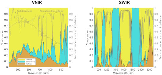
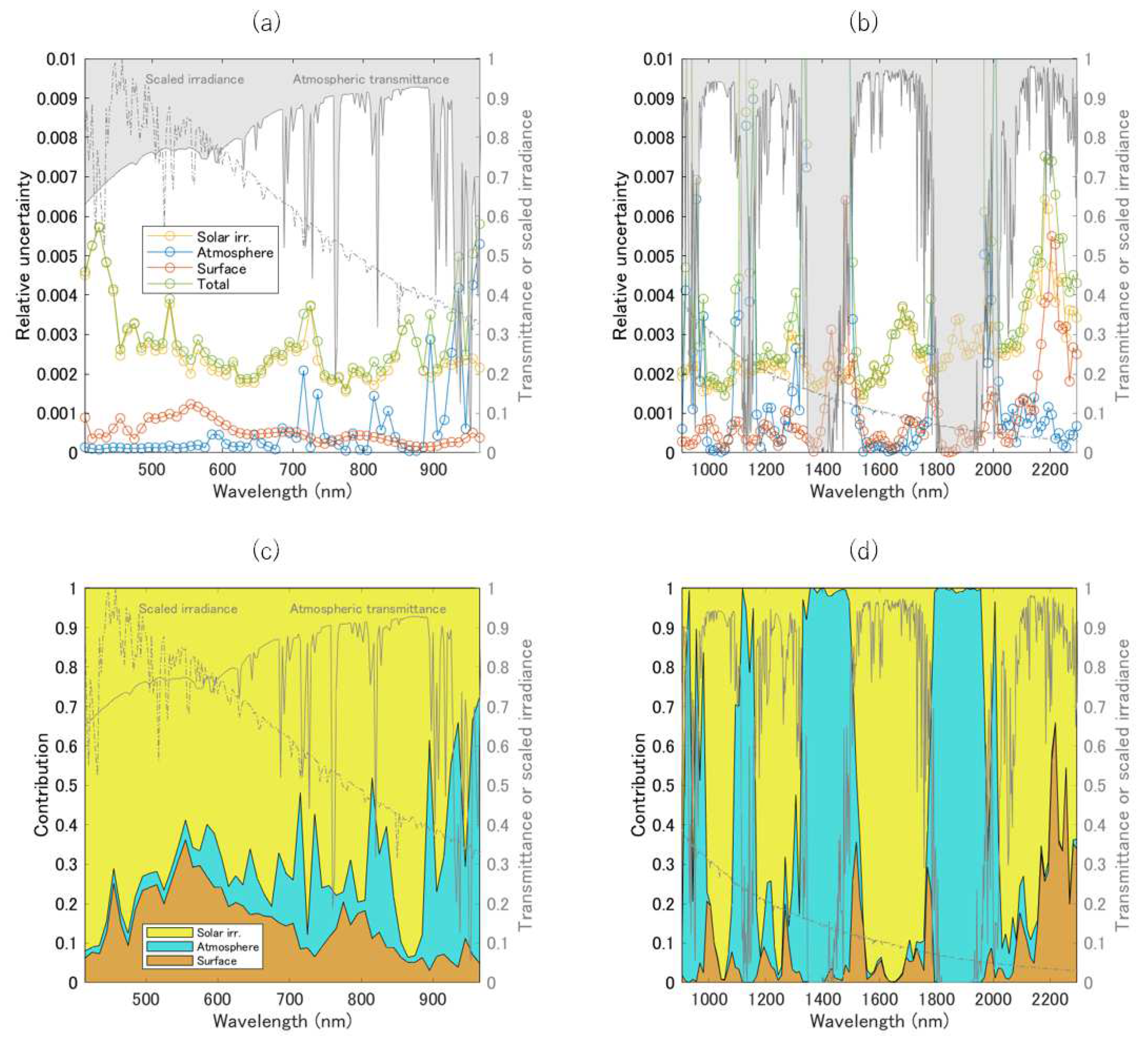
The uncertainty in each layer and the total uncertainty in the VNIR bands for Case-1 of the solar irradiance uncertainty are shown in Figure 4a. The scaled solar irradiance spectrum and the products of the total upward and downward transmittances are plotted to reveal the relationships between the parameters and uncertainties. The scaled solar irradiance, denoted by a gray dash-dot line, was derived by interpolating the kurucz2005 solar irradiance (No. 12 in Table 2) into 2.5 nm resolution, followed by normalization. The product of the atmospheric transmittance spectra, denoted by a gray line, corresponds to the simulated results obtained from MODTRAN interpolated into 2.5 nm resolution.
The values of the total uncertainties ranged from 0.002 (0.2%) to 0.006 (0.6%) (Figure 4a). Bands that were affected by atmospheric absorption and fluctuations in the solar irradiance showed relatively higher values. Figure 4c shows the relative contributions of the uncertainties for each layer (relative values of , , and ). Overall, the effects of the exo-atmospheric layer, i.e., the solar irradiance uncertainty, dominated the effects of the other two layers. The effects of the solar irradiance uncertainty and the soil line coefficients, i.e., the surface reflectance spectral variability, were greater at shorter wavelengths, especially between 500 nm and 650 nm. The effects of the uncertainty in the atmospheric parameters gradually increased with the wavelength and showed a greater contribution to the wavelength in the presence of strong atmospheric absorption. The wavelength region between 840 nm and 900 nm, used for remote sensing of vegetation, was significantly affected by the solar irradiance uncertainty. The effects of the soil line coefficients were smaller at longer wavelengths because the soil reflectance tended to be less wavelength-dependent than it was at shorter wavelengths.
The uncertainties in each layer and the total uncertainty in the SWIR bands for Case-1 of solar irradiance uncertainty are shown in Figure 4b. The value of the total uncertainty ranged from 0.0015 (0.15%) to 0.008 (0.8%) in the bands less affected by atmospheric absorption. Relatively large errors were identified at wavelengths exceeding 2100 nm, at which the effects of the surface reflectance and solar irradiance were dominant. Figure 4d shows the relative contributions of each layer in the SWIR band region. In wavelength regions corresponding to atmospheric windows of less than 2100 nm, the effects of the solar irradiance were greatest, followed by the effects of the surface reflectance. A effects were very small in these regions (e.g., 1600–1700 nm). The relative contributions of the uncertainties in the wavelength region between 2100 and 2300 nm are clearly identified in Figure 4d, revealing that the surface reflectance and solar irradiance effects were greater than the effects of the atmospheric spectra, and that the atmospheric effect was small.
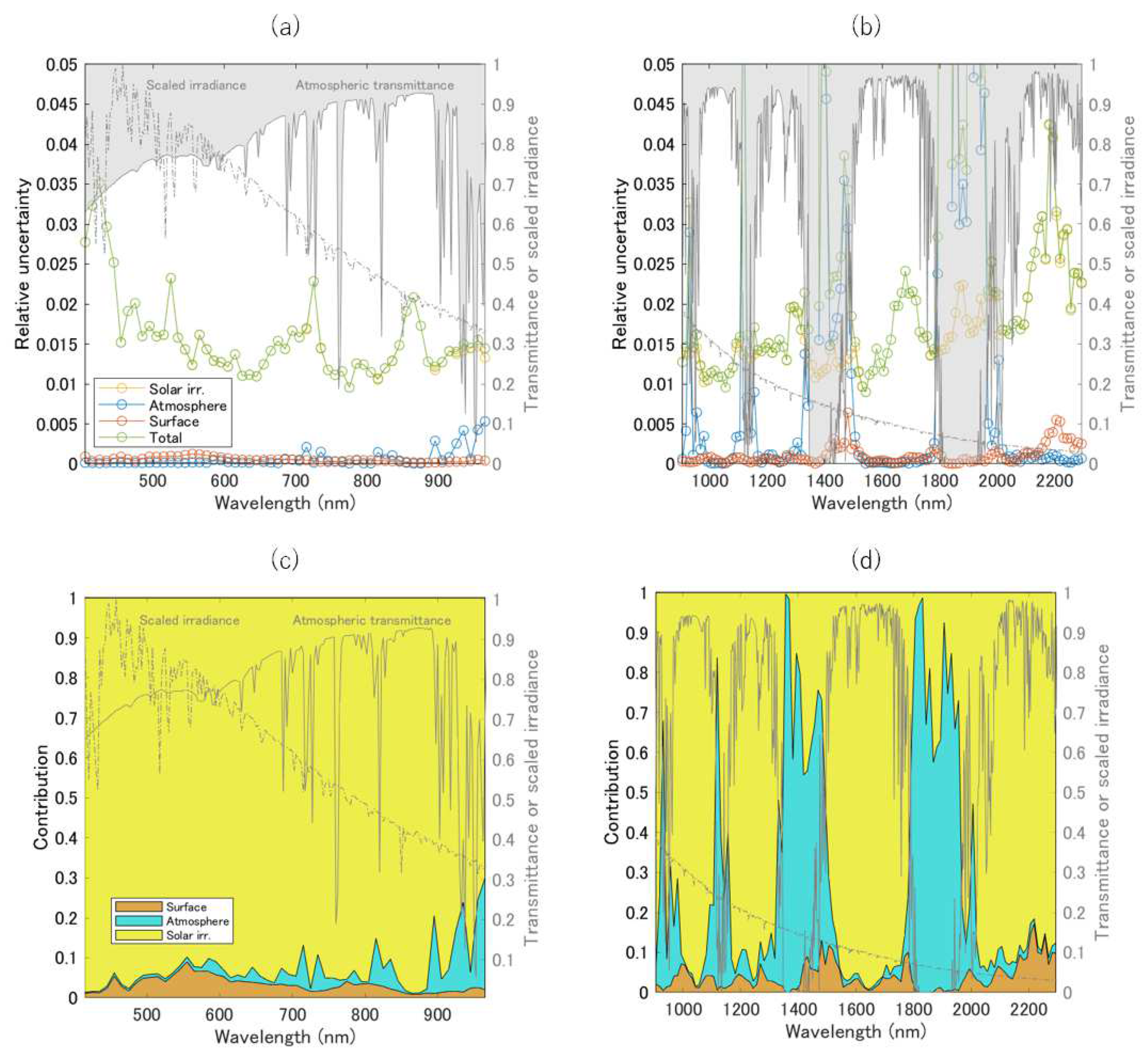
Figure 5a,c shows the approximations of the uncertainties and the relative contributions to the VNIR band for Case-2. The total uncertainty ranged from 0.01 and 0.04 (1% and 4%). Solar irradiance effects were much higher than the effects of the other layers in this case. Figure 5b,d shows the results obtained in the SWIR band. The total uncertainty ranged from 0.01 and 0.045 (1% and 4.5%) in the atmospheric window. The solar irradiance effects were high, as shown in Figure 5d.
4.2. Evaluation of the Derived Equation
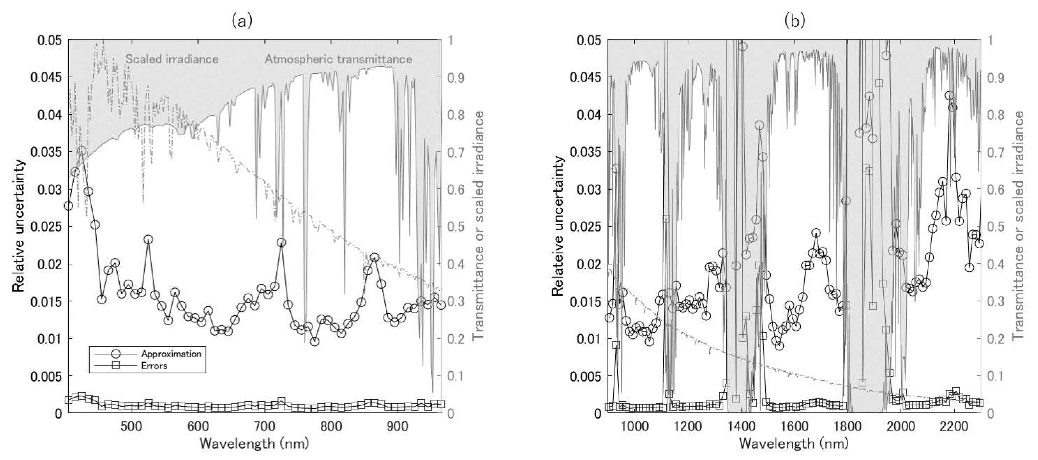
Errors in the approximations based on Equation (16) for the VNIR region were, in general, small relative to the approximations in the uncertainty, as shown in Figure 6a. The average error in the VNIR region of the approximation was 6.4%.
The results obtained from the SWIR region (Figure 6b) indicated that the errors were small relative to the approximated uncertainties, except for the strong atmospheric absorption bands. The average approximation error in the SWIR region was 6.3% when the product of the atmospheric transmittances exceeded 0.5. In the bands that were strongly affected by water vapor absorption, the approximation errors were significantly larger, possibly due to the lower correlation between the spectral matching band parameters.
5. Discussion
The relative contribution of the uncertainty in solar irradiance to the total uncertainty was higher than the contributions of the uncertainty in the spectral parameters for atmosphere and surfaces in the atmospheric windows over the entire spectral range examined. Even at the lower solar irradiance uncertainty level of 0.25% (Case-1), the effects were consistently high. These results can be attributed to the use of solar irradiance values in the conversion of reflectances to radiances. The uncertainty could be approximated using a single term, as represented in Equation (17), with no covariance terms; however, the effects of solar irradiance would be small in the radiance-to-radiance conversion because the covariance terms in Equation (11) cancel out. Therefore, the large effects of the solar irradiance uncertainty are unavoidable for the reflectance-to-radiance conversion, and the use of accurate irradiance models is key to obtaining accurate spectral band adjustments and intercalibrations.
Numerical simulations indicated that the total uncertainty ranged from <0.6% to <0.8% in the VNIR and SWIR bands, respectively, for atmospheric windows in Case-1 of solar irradiance uncertainties, whereas the total uncertainty was <4.0% to <4.5% in the VNIR and SWIR bands, respectively, for atmospheric windows in Case-2. The results for the uncertainty obtained in the present study correspond to a 68% confidence level (a coverage factor, k = 1) for a Gaussian distribution. The CPF radiometric accuracy of baseline is, however, 0.3% (k = 2) at 700–1000 nm and 1% (k = 2) at 350–2300 nm, smaller than results obtained in the present study even though the coverage factor (k) was 2. The fact implies that the effects of uncertainties in spectral band adjustment are not negligible relative to the calibration accuracy when CPF is used as the reference sensor, even for Case-1.
The uncertainty approximation in Equation (16) was influenced by various factors and limitations. The higher-order terms in the statistics (e.g., skewness and kurtosis) were neglected; hence, the outputs were assumed to be Gaussian, an assumption that does not always apply. Additionally, the model describing the error propagation was based on a first-order Taylor series. Higher-order terms were neglected, although Equation (15) is not a linear function. Finally, all inputs were assumed to be Gaussian, even though this assumption does not always apply. The factors may have introduced errors into the uncertainty approximations, as shown in Figure 6. In addition, the atmospheric spectral parameters were not explicitly expressed as a function of AOT, CWV, and COA in the approximation of uncertainties. Such expression would be more appropriate to understand the relationships between the uncertainties in the inputs and outputs [32]; however, it would be complicated for use in the first step of the derivation, and current forms of the derivation are satisfactory for addressing the objective and obtaining the results and insights presented in this study.
The results obtained in the present study are specific to the parameter settings of the spectral band configuration, selected solar irradiance model, atmospheric model, magnitude of the input errors of the atmospheric variables, and selected spectral surface reflectances. Changes in these conditions can alter the results, but the insights obtained from the results are generally applicable if conditions are not significantly different from those used in the simulations.
The framework of the present study is applicable not only to reflectance-to-radiance conversion, but also to reflectance-to-reflectance and radiance-to-radiance conversions. For example, the German hyperspectral sensor onboard the ISS, DESIS, provides radiance products [2]. Intercalibration between HISUI and DESIS [7] requires the radiance-to-radiance conversion of the spectral band adjustment, and the uncertainty could be evaluated using the equations derived in the present study (Equations (10)–(13)).
In intercalibration between hyperspectral sensors, sources of uncertainty include radiometric and spectral calibration uncertainties, the effects of differences in the spatial resolution, relative geolocation errors, and polarization sensitivity differences, among others. Specifically, the geometric accuracy of the products of the sensors on the ISS may be low compared with the accuracies of satellites flying at around 700 km, because the ISS experiences large variations in attitude and altitude [57]. The magnitudes of these effects on intercalibration should be investigated in a separate study.
6. Conclusions
The effects of the uncertainties in the spectral parameters of each layer on the results of spectral band adjustment were derived using the theory of error propagation. The derived results reveal that the keys to understanding the uncertainty in spectral band adjustment were the magnitudes of the errors in the parameters and the correlations between parameters within each layer. The small errors in spectral band adjustment obtained using two-way atmospheric radiative transfer code, reported in previous studies [19,20], were attributed to the covariance terms that cancel out the uncertainty and lead to small errors in the derived results.
A sensitivity analysis using the derived equations provided information about the relative contributions of each layer to the total uncertainty for the spectral band adjustment between CPF and HISUI. The effects of the solar irradiance dominated the atmospheric window, whereas the effects of the atmosphere and surface were relatively small. The findings indicate that accurate estimates of atmospheric parameters, such as AOT, CWV, and COA, are not needed. In addition, in-situ measurements of hyperspectral surface reflectances for soil surfaces are not required. The findings should be useful when devising methods for spectral band adjustment as well as intercalibration. Consequently, measuring solar irradiance with high accuracy is important for the spectral band adjustment of hyperspectral sensors, especially for reflectance-to-radiance conversion.
Funding
This research received no external funding.
Acknowledgments
The present study was supported by the Ministry of Economy, Trading and Industry of Japan (METI). The author is grateful to the HISUI calibration working group and to people related to the HISUI project for their support. Solar irradiance data from Arvesen [39] and Colina [41] were downloaded from the SOLID (First European SOLar Irradiance Data Exploitation) project website (http://projects.pmodwrc.ch/solid/). Wehrli [40] and ASTM [42] irradiance data were downloaded from the website of the U.S. N Renewable Energy Laboratory (https://www.nrel.gov/grid/solar-resource/spectra.html). Fontenla [45] irradiance data were downloaded from the website of the Solar Radiation Physical Modeling (SRPM) [51]. NRLSSI2 irradiance data were downloaded from the website of the Naval Research Laboratory (https://www.ncei.noaa.gov/data/spectral-solar-irradiance/access/ancillary-data/). SAGTIRE-S data were downloaded from the website of the Max Planck Institute for Solar System Research (http://www2.mps.mpg.de/projects/sun-climate/data.html). SOLAR-ISS data were downloaded from the web page http://bdap.ipsl.fr/voscat/SOLAR_ISS_V1.html.
Conflicts of Interest
The author declares no conflicts of interest.
Appendix A. Partial Derivatives of the Errors Propagated during the Radiance/Reflectance-to- Radiance Conversion
References
- Foerster, S.; Guanter, L.; Lopez, T.; Moreno, J.; Rast, M.; Schaepman, M.E. Guest Editorial: International Space Science Institute (ISSI) Workshop on Space-Borne Imaging Spectroscopy for Exploring the Earth’s Ecosystems. Surv. Geophys. 2019, 40, 297–301. [Google Scholar] [CrossRef]
- Müller, R.; Bachmann, M.; Alonso, K.; Carmona, E.; Cerra, D.; los Reyes, R.D.; Gerasch, B.; Krawczyk, H.; Ziel, V.; Heiden, U.; et al. Processing, Validation And Quality Control Of Spaceborne Imaging Spectroscopy Data From DESIS Mission on the ISS. In Proceedings of the IGARSS 2018—2018 IEEE International Geoscience and Remote Sensing Symposium, Valencia, Spain, 22–27 July 2018; pp. 189–191. [Google Scholar] [CrossRef]
- Matsunaga, T.; Iwasaki, A.; Tsuchida, S.; Iwao, K.; Nakamura, R.; Yamamoto, H.; Kato, S.; Obata, K.; Kashimura, O.; Tanii, J.; et al. HISUI Status Toward FY2019 Launch. In Proceedings of the IGARSS 2018—2018 IEEE International Geoscience and Remote Sensing Symposium, Valencia, Spain, 22–27 July 2018; pp. 160–163. [Google Scholar] [CrossRef]
- Green, R.O. The Earth Surface Mineral Dust Source Investigation (EMIT). Available online: https://hyspiri.jpl.nasa.gov/downloads/2018_Workshop/day1/13_HyspIRI_EMIT_Overview_20180815b.pdf (accessed on 19 April 2019).
- CLARREO Pathfinder Mission Team. Pathfinder Mission for Climate Absolute Radiance and Refractivity Observatory (CLARREO); Technical Report; National Aeronautics and Space Administration: Washington, DC, USA, 2016.
- Obata, K.; Tsuchida, S.; Nagatani, I.; Yamamoto, H.; Kouyama, T.; Yamada, Y.; Yamaguchi, Y.; Ishii, J. An overview of ISS HISUI hyperspectral imager radiometric calibration. In Proceedings of the IGARSS 2018—2018 IEEE International Geoscience and Remote Sensing Symposium, Beijing, China, 10–15 July 2016; pp. 1924–1927. [Google Scholar] [CrossRef]
- Yamamoto, H.; Obata, K.; Tsuchida, S.; Kerr, G.; Bachmann, M. Cross-sensor calibration and validation between DESIS and HISUI Hyperspectral Imager on the International Space Station (ISS). In Proceedings of the 2016 IEEE International Geoscience and Remote Sensing Symposium (IGARSS), Beijing, China, 10–15 July 2016; pp. 1928–1930. [Google Scholar] [CrossRef]
- Chander, G.; Markham, B.L.; Barsi, J.A. Revised Landsat-5 Thematic Mapper Radiometric Calibration. IEEE Geosci. Remote Sens. Lett. 2007, 4, 490–494. [Google Scholar] [CrossRef]
- Chander, G.; Mishra, N.; Helder, D.L.; Aaron, D.B.; Angal, A.; Choi, T.; Xiong, X.; Doelling, D.R. Applications of Spectral Band Adjustment Factors (SBAF) for Cross-Calibration. IEEE Trans. Geosci. Remote Sens. 2013, 51, 1267–1281. [Google Scholar] [CrossRef]
- Lukashin, C.; Wielicki, B.A.; Young, D.F.; Thome, K.; Jin, Z.; Sun, W. Uncertainty Estimates for Imager Reference Inter-Calibration With CLARREO Reflected Solar Spectrometer. IEEE Trans. Geosci. Remote Sens. 2013, 51, 1425–1436. [Google Scholar] [CrossRef]
- Roithmayr, C.M.; Lukashin, C.; Speth, P.W.; Kopp, G.; Thome, K.; Wielicki, B.A.; Young, D.F. CLARREO Approach for Reference Intercalibration of Reflected Solar Sensors: On-Orbit Data Matching and Sampling. IEEE Trans. Geosci. Remote Sens. 2014, 52, 6762–6774. [Google Scholar] [CrossRef] [Green Version]
- Wu, A.; Xiong, X.; Jin, Z.; Lukashin, C.; Wenny, B.N.; Butler, J.J. Sensitivity of Intercalibration Uncertainty of the CLARREO Reflected Solar Spectrometer Features. IEEE Trans. Geosci. Remote Sens. 2015, 53, 4741–4751. [Google Scholar] [CrossRef]
- Lukashin, C.; Jin, Z.; Kopp, G.; MacDonnell, D.G.; Thome, K. CLARREO Reflected Solar Spectrometer: Restrictions for Instrument Sensitivity to Polarization. IEEE Trans. Geosci. Remote Sens. 2015, 53, 6703–6709. [Google Scholar] [CrossRef]
- Teillet, P.; Barker, J.; Markham, B.; Irish, R.; Fedosejevs, G.; Storey, J. Radiometric cross-calibration of the Landsat-7 ETM+ and Landsat-5 TM sensors based on tandem data sets. Remote Sens. Environ. 2001, 78, 39–54. [Google Scholar] [CrossRef] [Green Version]
- Mishra, N.; Haque, M.O.; Leigh, L.; Aaron, D.; Helder, D.; Markham, B. Radiometric Cross Calibration of Landsat 8 Operational Land Imager (OLI) and Landsat 7 Enhanced Thematic Mapper Plus (ETM+). Remote Sens. 2014, 6, 12619–12638. [Google Scholar] [CrossRef] [Green Version]
- Uprety, S.; Cao, C. Suomi NPP VIIRS reflective solar band on-orbit radiometric stability and accuracy assessment using desert and Antarctica Dome C sites. Remote Sens. Environ. 2015, 166, 106–115. [Google Scholar] [CrossRef]
- Barrientos, C.; Mattar, C.; Nakos, T.; Perez, W. Radiometric Cross-Calibration of the Chilean Satellite FASat-C Using RapidEye and EO-1 Hyperion Data and a Simultaneous Nadir Overpass Approach. Remote Sens. 2016, 8, 612. [Google Scholar] [CrossRef]
- Doelling, D.R.; Lukashin, C.; Minnis, P.; Scarino, B.; Morstad, D. Spectral Reflectance Corrections for Satellite Intercalibrations Using SCIAMACHY Data. IEEE Geosci. Remote Sens. Lett. 2012, 9, 119–123. [Google Scholar] [CrossRef]
- Obata, K.; Tsuchida, S.; Yamamoto, H.; Thome, K. Cross-Calibration between ASTER and MODIS Visible to Near-Infrared Bands for Improvement of ASTER Radiometric Calibration. Sensors 2017, 17, 1793. [Google Scholar] [CrossRef] [PubMed]
- Teillet, P.; Slater, P.; Ding, Y.; Santer, R.; Jackson, R.; Moran, M. Three methods for the absolute calibration of the NOAA AVHRR sensors in-flight. Remote Sens. Environ. 1990, 31, 105–120. [Google Scholar] [CrossRef]
- Thome, K.J.; Biggar, S.F.; Wisniewski, W. Cross comparison of EO-1 sensors and other Earth resources sensors to Landsat-7 ETM+ using Railroad Valley Playa. IEEE Trans. Geosci. Remote Sens. 2003, 41, 1180–1188. [Google Scholar] [CrossRef]
- Lacherade, S.; Fougnie, B.; Henry, P.; Gamet, P. Cross Calibration Over Desert Sites: Description, Methodology, and Operational Implementation. IEEE Trans. Geosci. Remote Sens. 2013, 51, 1098–1113. [Google Scholar] [CrossRef]
- Verhoef, W.; Bach, H. Simulation of hyperspectral and directional radiance images using coupled biophysical and atmospheric radiative transfer models. Remote Sens. Environ. 2003, 87, 23–41. [Google Scholar] [CrossRef]
- Mousivand, A.; Verhoef, W.; Menenti, M.; Gorte, B. Modeling Top of Atmosphere Radiance over Heterogeneous Non-Lambertian Rugged Terrain. Remote Sens. 2015, 7, 8019–8044. [Google Scholar] [CrossRef] [Green Version]
- Yoshioka, H. Vegetation isoline equations for an atmosphere-canopy-soil system. IEEE Trans. Geosci. Remote Sens. 2004, 42, 166–175. [Google Scholar] [CrossRef]
- Baret, F.; Jacquemoud, S.; Hanocq, J. About the soil line concept in remote sensing. Adv. Space Res. 1993, 13, 281–284. [Google Scholar] [CrossRef]
- Yoshioka, H.; Huete, A.R.; Miura, T. Derivation of vegetation isoline equations in red-NIR reflectance space. IEEE Trans. Geosci. Remote Sens. 2000, 38, 838–848. [Google Scholar] [CrossRef]
- Yoshioka, H.; Miura, T.; Huete, A.; Ganapol, B. Analysis of Vegetation Isolines in Red-NIR Reflectance Space. Remote Sens. Environ. 2000, 74, 313–326. [Google Scholar] [CrossRef]
- Miura, M.; Obata, K.; Yoshioka, H. Vegetation isoline equations with first- and second-order interaction terms for modeling a canopy-soil system of layers in the red and near-infrared reflectance space. J. Appl. Remote Sens. 2015, 9, 095987. [Google Scholar] [CrossRef]
- Miura, M.; Obata, K.; Taniguchi, K.; Yoshioka, H. Improved Accuracy of the Asymmetric Second-Order Vegetation Isoline Equation over the RED-NIR Reflectance Space. Sensors 2017, 17, 450. [Google Scholar] [CrossRef] [PubMed]
- Obata, K.; Miura, T.; Yoshioka, H.; Huete, A.R. Derivation of a MODIS-compatible enhanced vegetation index from visible infrared imaging radiometer suite spectral reflectances using vegetation isoline equations. J. Appl. Remote Sens. 2013, 7, 073467. [Google Scholar] [CrossRef] [Green Version]
- Fan, X.; Liu, Y. Quantifying the Relationship Between Intersensor Images in Solar Reflective Bands: Implications for Intercalibration. IEEE Trans. Geosci. Remote Sens. 2014, 52, 7727–7737. [Google Scholar]
- Fan, X.; Liu, Y. A Generalized Model for Intersensor NDVI Calibration and Its Comparison With Regression Approaches. IEEE Trans. Geosci. Remote Sens. 2017, 55, 1842–1852. [Google Scholar] [CrossRef]
- Fan, X.; Liu, Y. Multisensor Normalized Difference Vegetation Index Intercalibration: A Comprehensive Overview of the Causes of and Solutions for Multisensor Differences. IEEE Geosci. Remote Sens. Mag. 2018, 6, 23–45. [Google Scholar] [CrossRef]
- Taylor, J.R. An Introduction to Error Analysis: The Study of Uncertainties in Physical Measurements, 2nd ed.; University Science Books: Mill Valley, CA, USA, 1997. [Google Scholar]
- Currey, C.; Bartle, A.; Lukashin, C.; Roithmayr, C.; Gallagher, J. Multi-Instrument Inter-Calibration (MIIC) System. Remote Sens. 2016, 8, 902. [Google Scholar] [CrossRef]
- Tanii, J.; Kashimura, O.; Ito, Y.; Iwasaki, A. Flight model performances of HISUI hyperspectral sensor onboard ISS (International Space Station). In Proceedings of the Sensors, Systems, and Next-Generation Satellites XX, Edinburgh, UK, 26–29 September 2016; Volume 10000, p. 104230Q. [Google Scholar] [CrossRef]
- Ogawa, K.; Konno, Y.; Yamamoto, S.; Matsunaga, T.; Tachikawa, T.; Komoda, M. Observation planning algorithm of a Japanese space-borne sensor: Hyperspectral Imager SUIte (HISUI) onboard International Space Station (ISS) as platform. In Proceedings of the Sensors, Systems, and Next-Generation Satellites XXI, Warsaw, Poland, 11–14 September 2017; Volume 10423. [Google Scholar]
- Arvesen, J.C.; Griffin, R.N.; Pearson, B.D. Determination of Extraterrestrial Solar Spectral Irradiance from a Research Aircraft. Appl. Opt. 1969, 8, 2215–2232. [Google Scholar] [CrossRef] [PubMed]
- Wehrli, C. Extraterrestrial Solar Spectrum. Publication No. 615, Physikalisch Meteorologisches Observatorium Davos + World Radiation Center (PMOD/WRC); PMOD/WRC: Davos Dorf, Switzerland, 1985. [Google Scholar]
- Colina, L.; Bohlin, R.C.; Castelli, F. The 0.12-2.5 micron Absolute Flux Distribution of the Sun for Comparison With Solar Analog Stars. Astron. J. 1996, 8, 307–315. [Google Scholar] [CrossRef]
- American Society for Testing and Materials. Standard Solar Constant and Zero Air Mass Solar Spectral Irradiance Tables. Standard E490-00. 2000. Available online: http://rredc.nrel.gov/solar/spectra/am0/ASTM2000.html (accessed on 15 December 2017).
- Thuillier, G.; Hersé, M.; Labs, D.; Foujols, T.; Peetermans, W.; Gillotay, D.; Simon, P.; Mandel, H. The Solar Spectral Irradiance from 200 to 2400 nm as Measured by the SOLSPEC Spectrometer from the Atlas and Eureca Missions. Sol. Phys. 2003, 214, 1–22. [Google Scholar] [CrossRef]
- Gueymard, C.A. The sun’s total and spectral irradiance for solar energy applications and solar radiation models. Sol. Energy 2004, 76, 423–453. [Google Scholar] [CrossRef]
- Fontenla, J.M.; Harder, J.; Livingston, W.; Snow, M.; Woods, T. High-resolution solar spectral irradiance from extreme ultraviolet to far infrared. J. Geophys. Res. Atmos. 2011, 116, D20108. [Google Scholar] [CrossRef]
- Coddington, O.; Lean, J.L.; Pilewskie, P.; Snow, M.; Lindholm, D. A Solar Irradiance Climate Data Record. Bull. Am. Meteorol. Soc. 2016, 97, 1265–1282. [Google Scholar] [CrossRef]
- Yeo, K.L.; Krivova, N.A.; Solanki, S.K.; Glassmeier, K.H. Reconstruction of total and spectral solar irradiance from 1974 to 2013 based on KPVT, SoHO/MDI, and SDO/HMI observations. Astron. Astrophys. 2014, 570, A85. [Google Scholar] [CrossRef] [Green Version]
- Meftah, M.; Damé, L.; Bolsée, D.; Hauchecorne, A.; Pereira, N.; Sluse, D.; Cessateur, G.; Irbah, A.; Bureau, J.; Weber, M.; et al. SOLAR-ISS: A new reference spectrum based on SOLAR/SOLSPEC observations. Astron. Astrophys. 2018, 611, A1. [Google Scholar] [CrossRef]
- Berk, A.; Anderson, G.; Acharya, P.; Shettle, E. MODTRAN 5.2.1 User’s Manual; Spectral Sciences, Inc.: Burlington, MA, USA, 2011. [Google Scholar]
- Berk, A.; Anderson, G.P.; Acharya, P.K.; Bernstein, L.S.; Muratov, L.; Lee, J.; Fox, M.; Adler-Golden, S.M.; Chetwynd, J.H.; Hoke, M.L.; et al. MODTRAN 5: A reformulated atmospheric band model with auxiliary species and practical multiple scattering options: Update. In Proceedings of the Algorithms and Technologies for Multispectral, Hyperspectral, and Ultraspectral Imagery XI, Orlando, FL, USA, 28 March–1 April 2005; Volume 5806, pp. 662–668. [Google Scholar] [CrossRef]
- Fontenla, J. Solar Radiation Physical Modeling (SRPM). 2000. Available online: http://www.digidyna.com/Results2010/spectra/irradiance/index_spectra_irradiance.html (accessed on 15 December 2017).
- Ball, W.T.; Krivova, N.A.; Unruh, Y.C.; Haigh, J.D.; Solanki, S.K. A New SATIRE-S Spectral Solar Irradiance Reconstruction for Solar Cycles 21-23 and Its Implications for Stratospheric Ozone. J. Atmos. Sci. 2014, 71, 4086–4101. [Google Scholar] [CrossRef]
- Clark, R.; Swayze, G.; Wise, R.; Livo, E.; Hoefen, T.; Kokaly, R.; Sutley, S. USGS Digital Spectral Library Splib06a: U.S. Geological Survey, Digital Data Series 231. Available online: http://speclab.cr.usgs.gov/spectral.lib06 (accessed on 15 December 2017).
- Gao, B.C.; Kaufman, Y. The MODIS Near-IR Water Vapor Algorithm; NASA: Washington, DC, USA, 1998.
- Levy, R.C.; Mattoo, S.; Munchak, L.A.; Remer, L.A.; Sayer, A.M.; Patadia, F.; Hsu, N.C. The Collection 6 MODIS aerosol products over land and ocean. Atmos. Meas. Tech. 2013, 6, 2989–3034. [Google Scholar] [CrossRef] [Green Version]
- Borbas, E.; Seemann, S.; Kern, A.; Moy, L.; Li, J.; Gumley, L.; Menzel, W. MODIS Atmospheric Profile Retrieval Algorithm Theoretical Basis Document Collection 6; University of Wisconsin0Madison: Madison, WI, USA, 2011. [Google Scholar]
- Dou, C.; Zhang, X.; Guo, H.; Han, C.; Liu, M. Improving the Geolocation Algorithm for Sensors Onboard the ISS: Effect of Drift Angle. Remote Sens. 2014, 6, 4647–4659. [Google Scholar] [CrossRef] [Green Version]
Figure 1.
Illustration of model-based spectral band adjustment, including the conversion between radiance and reflectance.
Figure 1.
Illustration of model-based spectral band adjustment, including the conversion between radiance and reflectance.

Figure 2.
Relative differences between the 15 solar irradiances listed in Table 2 and their mean (each irradiance minus mean).
Figure 2.
Relative differences between the 15 solar irradiances listed in Table 2 and their mean (each irradiance minus mean).
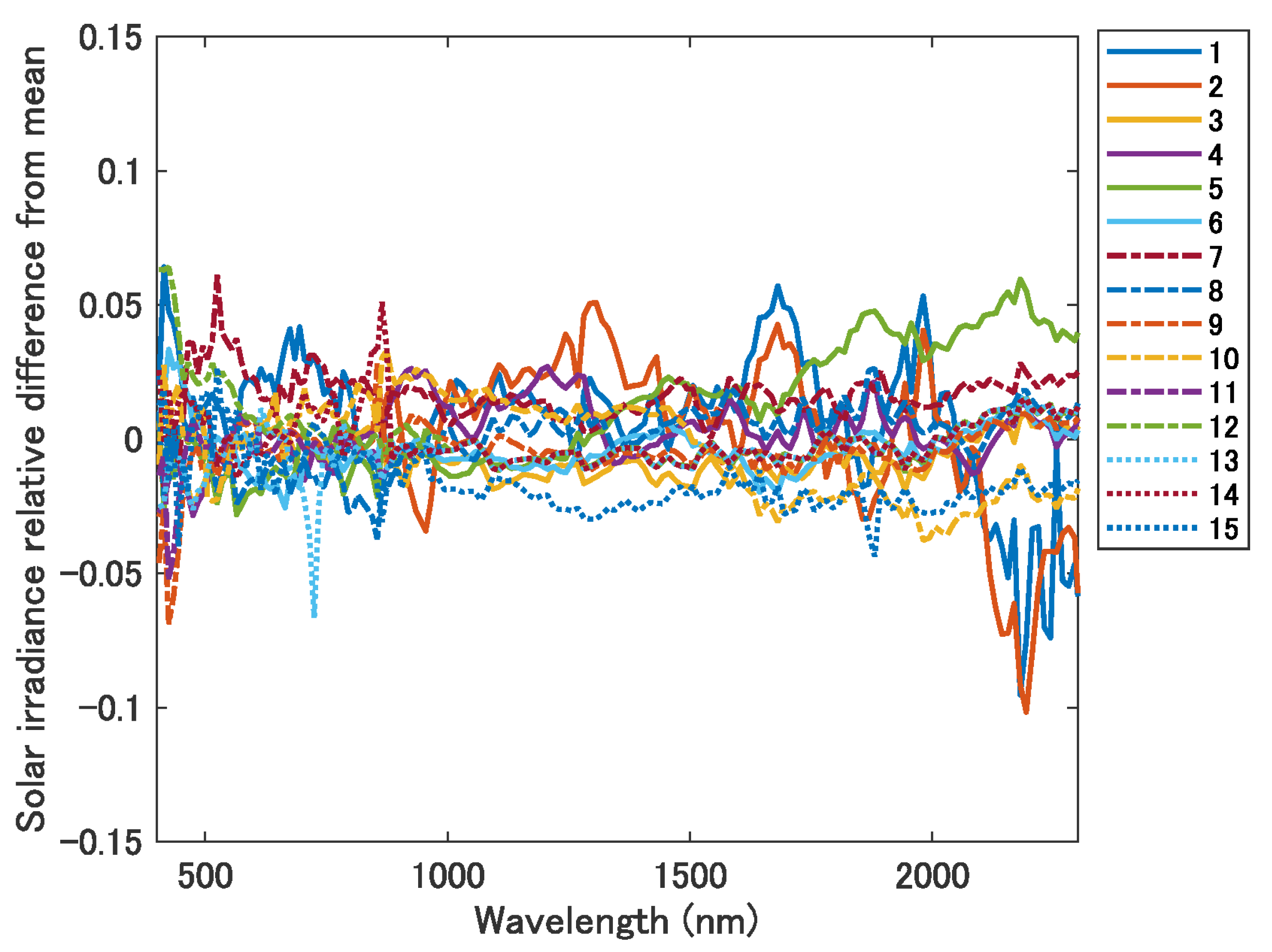
Figure 3.
Reflectance samples for soil, rocks, and their mixtures obtained from the USGS spectral library [53].
Figure 3.
Reflectance samples for soil, rocks, and their mixtures obtained from the USGS spectral library [53].
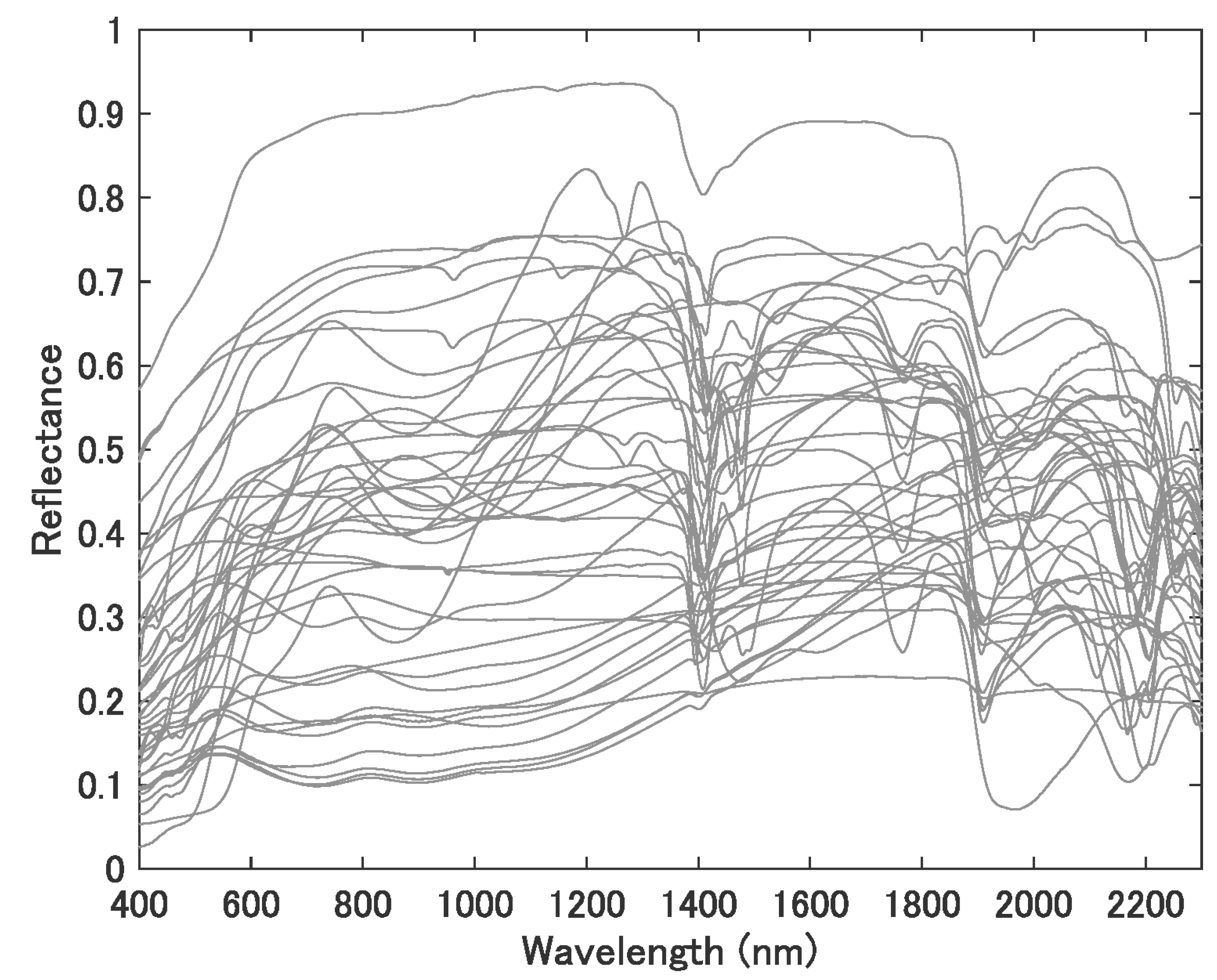
Figure 4.
(a) Plot of the approximated uncertainties in the relative values obtained from each layer (exo-atmosphere, atmosphere, and surface) and the total uncertainties of the approximations in relative values for the HISUI VNIR band region at a lower standard deviation for the solar irradiance models (Case-1). (b) The same plot for the HISUI SWIR region (<2300 nm). (c) Plot of the relative contributions of the uncertainties in each layer to the total uncertainties in the VNIR region for Case-1 of the solar irradiance model. (d) The same plot for the SWIR region (<2300 nm).

Figure 5.
(a) Plot of the approximated uncertainties in the relative values from each layer (exo-atmosphere, atmosphere, and surface) and the total uncertainties in the approximations of the relative values for the HISUI VNIR band region at a higher standard deviation in the solar irradiance models (Case-2). (b) The same plot for the HISUI SWIR region (<2300 nm). (c) Plot of the relative contributions of the uncertainties in each layer to the total uncertainties in the VNIR region for Case-2 of the solar irradiance model. (d) The same plot for the SWIR region (<2300 nm).

Figure 6.
(a) Plot of the uncertainty approximation in the relative values using the derived equation (Equation (16)) for the HISUI VNIR band region. The absolute differences between approximated and simulated uncertainties in the relative values are also shown. (b) Plot of the approximated uncertainties and absolute errors between approximated and simulated uncertainties in the relative values of the HISUI SWIR band region (<2300 nm).


| CLARREO Pathfinder | HISUI | |
|---|---|---|
| Mission lifetime | 1–2 years | 3 years |
| Spectral range | 350–2300 nm | 400–2500 nm |
| Spectral resolution | 4 nm sampling and 8 nm bandwidth (baseline) | 10 nm in VNIR |
| 8 nm sampling and 16 nm bandwidth (threshold) | 12.5 nm in SWIR | |
| Spatial resolution | 500 m | 30 m (AT) by 20 m (CT) |
| Swath width | 70 km | 20 km |
| Radiometric accuracy | 0.3% () at 700–1000 nm (baseline) | 5% |
| 1% () at 700–1000 nm (threshold) | ||
| 1% () at 350–2300 nm (baseline) | ||
| 3% () at 350–2300 nm (threshold) | ||
| Spectral accuracy | 1% () (baseline) and 2% () (threshold) | 0.2 nm in VNIR |
| 0.625 nm in SWIR |
CT means cross-track and AT means along-track. means a 95% confidence level (2) for a Gaussian distribution [5].
Table 2.
List of the spectral solar irradiances. Nos. 11–15 are based on spectral solar irradiances available at MODTRAN 5.2 [49,50].
| No. | Author | Year | Range (nm) | Interval (nm) | Solar Constant (W/m) |
| 1 | Arvesen [39] | 1969 | 300–2495 | 0.1 to 5 | - |
| 2 | Wehrli [40] | 1985 | 200–100,075 | 1 to 25 (≤2642.5) | 1367.0 |
| 3 | Colina [41] | 1996 | 120–2500 | 1 to 2 | - |
| 4 | ASTM [42] | 2000 | 120–100,000 | 1 to 2 (≤2500) | 1366.1 |
| 5 | Thuiller [43] | 2003 | 200–2400 | 0.1 to 1 | - |
| 6 | Gueymard [44] | 2004 | 0.5–1,000,000 | 1 to 5 (≤4000) | 1366.1 |
| 7 | Fontenla [45] | 2011 | 201–100,077 | 0.2 | 1379.91 |
| 8 | Coddington (NRLSSI2) [46] | 2016 | 115–100,000 | 1 | 1360.45 |
| 9 | Yeo (SATIRE-S) [47] | 2017 | 115–160,000 | 2 to 10 (≤3185) | 1372.3 |
| 10 | Meftath (SOLAR-ISS) [48] | 2017 | 0.5–3000 | 0.05–0.2 | - |
| No. | Product name | Year | Range (cm) | Interval (cm) | Solar constant (W/m) |
| 11 | SUN01kurucz1997 [49] | 1997 | 50–5000 | 1 | 1368.2 |
| 12 | SUN01kurukz2005 [49] | 2005 | 0–5000 | 1 | 1400.7 |
| 13 | SUN01chkur [49] | - | 50–5000 | 1 | 1359.75 |
| 14 | SUN01thkur [49] | - | 50–5000 | 1 | 1376.73 |
| 15 | SUN01fontenla [49] | - | 50–5000 | 1 | 1361.0 |
The values of each characteristic varied with the features of the data available at [51]. The present study employed irradiance spectra obtained when the Sun was covered by Model 1001 (feature B) at 1 nm resolution and 0.2 nm sampling. The value of the solar constant corresponded to the low activity case [45]. Spectral solar irradiances used in the present study were obtained from the SATIRE-S data (version date 20170610). Three-month averages of the data obtained between November 2008 and January 2009 involved the times of the Cycles 23–24 solar minima (December 2008) [52]. Version 1.1 (10-May-2017) was used. e The values of the solar constants were calculated by the author.
© 2019 by the author. Licensee MDPI, Basel, Switzerland. This article is an open access article distributed under the terms and conditions of the Creative Commons Attribution (CC BY) license (http://creativecommons.org/licenses/by/4.0/).
Share and Cite
MDPI and ACS Style
Obata, K. Sensitivity Analysis Method for Spectral Band Adjustment between Hyperspectral Sensors: A Case Study Using the CLARREO Pathfinder and HISUI. Remote Sens. 2019, 11, 1367. https://0-doi-org.brum.beds.ac.uk/10.3390/rs11111367
AMA Style
Obata K. Sensitivity Analysis Method for Spectral Band Adjustment between Hyperspectral Sensors: A Case Study Using the CLARREO Pathfinder and HISUI. Remote Sensing. 2019; 11(11):1367. https://0-doi-org.brum.beds.ac.uk/10.3390/rs11111367
Chicago/Turabian StyleObata, Kenta. 2019. "Sensitivity Analysis Method for Spectral Band Adjustment between Hyperspectral Sensors: A Case Study Using the CLARREO Pathfinder and HISUI" Remote Sensing 11, no. 11: 1367. https://0-doi-org.brum.beds.ac.uk/10.3390/rs11111367
Note that from the first issue of 2016, this journal uses article numbers instead of page numbers. See further details here.