Sub-Pixel Crop Type Classification Using PROBA-V 100 m NDVI Time Series and Reference Data from Sentinel-2 Classifications

Abstract

This paper presents the results of a sub-pixel classification of crop types in Bulgaria from PROBA-V 100 m normalized difference vegetation index (NDVI) time series. Two sub-pixel classification methods, artificial neural network (ANN) and support vector regression (SVR) were used where the output was a set of area fraction images (AFIs) at 100 m resolution with pixels containing estimated area fractions of each class. High-resolution maps of two test sites derived from Sentinel-2 classifications were used to obtain training data for the sub-pixel classifications. The estimated area fractions have a good correspondence with the true area fractions when aggregated to regions of 10 × 10 km², especially when the SVR method was used. For the five dominant classes in the test sites the R² obtained after the aggregation was 86% (winter cereals), 81% (sunflower), 92% (broad-leaved forest), 89% (maize), and 67% (grasslands) when the SVR method was used.

1. Introduction

One of the major benefits of low resolution sensors, such as SPOT-VEGETATION, MODIS (MODerate Resolution Imaging Spectroradiometer), and Sentinel-3, with respect to agricultural applications, is their temporal resolution, therefore the possibility to obtain (regular) time series of vegetation indices, such as normalized difference vegetation index (NDVI), throughout the growing season of crops. The data can be further derived to generate information either for crop growth status or for crop type discrimination and mapping, thanks to their distinct evolutive behaviors of reflectance related to their growth patterns. However, the applications are restricted by the coarse resolution of these sensors, and hence, the mixture of crop types within a single pixel. To overcome this problem a variety of sub-pixel classification methods have been proposed in literature.

The sub-pixel classification approach is also termed “soft” classification, as unlike the “hard” classification methods where each pixel is unambiguously assigned to one single class, it tries to reveal possible mixtures and define for each pixel the area fractions covered by the different cover classes [1]. Alternatively, instead of deriving area fractions of classes, similar softened classification output may be achieved by using posterior probabilities of class membership derived from maximum likelihood (MXL) classification [2,3]. Sub-pixel classification methods have been used in different contexts including crop area estimation [4,5], natural vegetation ecotone mapping [3,6], urban expansion [7], and change detection studies [8]. Different methods have been proposed for deriving sub-pixel class fractions including the linear mixture model (LMM) [4], artificial neural network (ANN) [9,10,11], regression tree [5], fuzzy classification [6,12], and support vector machine (SVM) [13].

Liu and Wu [11] argued that the non-linear models, especially neural network-based models, outperformed the traditional linear unmixing models. Support for such a conclusion is given in Verbeiren et al. [1] who compared ANN and LMM in an attempt to generate a sub-pixel map from SPOT-VEGETATION 1 km data across Belgium. The authors showed that the ANN approach outperformed LMM and that, for the major classes, the acreage estimates obtained via ANN, when aggregated to the level of the administrative regions, were in good agreement with the true values. Also, a multilayer perceptron (MLP) neural network regression algorithm has been shown to outperform the regression tree algorithm [5]. Atkinson et al. [9] also obtained better results with ANN than with the other tested methods but pointed out that its successful implementation depends on accurate co-registration and the availability of a training data set. Liu et al. [14] compared a linear spectral unmixing model, a supervised fully-fuzzy classification method and a SVM to generate a fraction map and achieved the most accurate fraction result using SVM. Six machine learning methods were compared in a recent study [15] based on multiple criteria, where the authors found that, in general, no method performs best for all evaluation criteria. However, when both time available for preprocessing and the magnitude of the training data set are unconstrained, support vector regression (SVR) and least-squares SVM for regression clearly outperform the other methods.

Regarding the satellite imagery widely used for agricultural monitoring, SPOT-VEGETATION (SPOT-VGT) sensors provided one of the longest time series of multispectral reflectance since 1998. The mission was succeeded in 2013 by PROBA-V (PRoject for On-Board Autonomy–Vegetation), a small satellite commissioned by the European Space Agency. The sensor on-board PROBA-V generates products at three different spatial resolutions: 1 km, 300 m and 100 m [16,17]. For agricultural applications, the 100 m product is of particular interest and has been shown useful for cropland and crop type mapping [18,19,20]. These studies used the traditional, hard classification approach where each pixel is assigned to one class. However, even with the improved spatial resolution of 100 m, the presence of mixed pixels may be a problem in agro-systems dominated by small fields [20]. It is thus meaningful to test the feasibility of the sub-pixel classification approach with the new PROBA-V 100 m data. Exhaustive testing and comparison of all possible sub-pixel classification methods is outside the scope of this study. Instead, we selected the ANN and the SVR methods as they have shown good results in previous studies for crop type area estimation, e.g., References [1,15].

Like all supervised approaches, the sub-pixel classification relies on ground truth data sampling. Ground sampling by field campaigns has to be designed following statistical principles, and therefore is onerous to be implemented. In a general circumstance, it provides data for a small number of spatially discontinuous polygons, which may not be sufficient for the training of a sub-pixel PROBA-V classification because pixels with different mixtures of classes must be included in the training samples. The area fractions for the training may be obtained, most conveniently, if we have high-resolution, wall-to-wall land-use datasets for one or more representative areas. These datasets may be obtained by classification of high-resolution satellite images for which purpose much smaller field datasets may be sufficient.

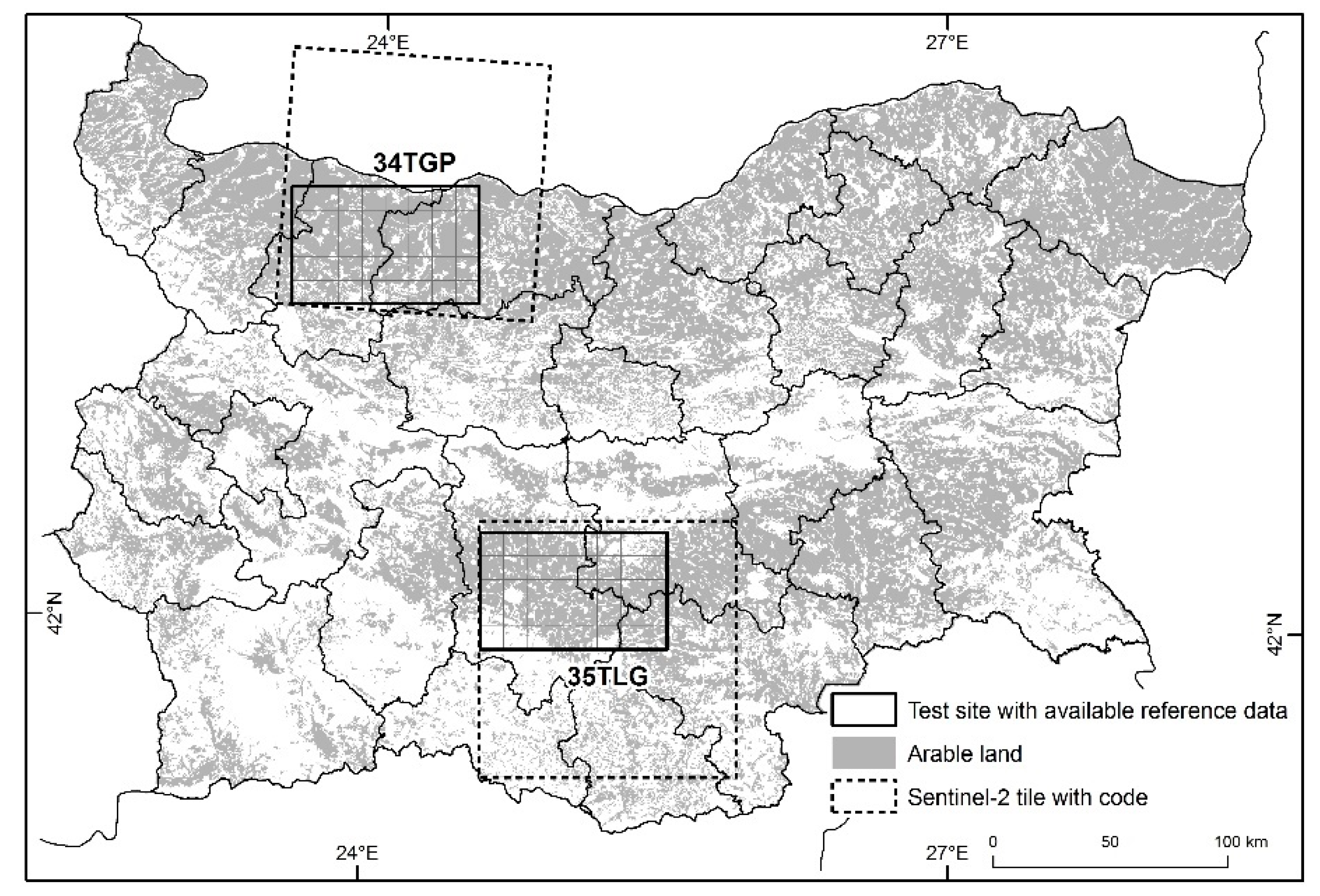
The general objective of this study was therefore to generate a sub-pixel crop (and land-use) map of Bulgaria using PROBA-V 100 m NDVI time series relying on a limited amount of ground reference data. To this aim, Sentinel-2 data was first used to produce a crop (and land-use) map at two test sites at 10 m spatial resolution. In a second stage, classification of the PROBA-V NDVI time series was performed using Sentinel-2 classifications results as training data. For Sentinel-2 classifications, two different input datasets, i.e., NDVI time series and multi-date cloud-free multi-spectral bands, as well as three different classifiers, i.e., maximum likelihood (MXL), SVM, and random forest (RF) were tested. The accuracy of the resulting Sentinel-2 maps was compared and the classification with the best results was used as reference dataset for training the PROBA-V classification.

2. Materials and Methods

2.1. Test Sites

Two test sites in Bulgaria, each covering area of ~80 × 50 km² (Figure 1) were selected to perform Sentinel-2 classifications and produce training data for the national level PROBA-V classification. The sites have artificially defined borders and their location was selected based on the following criteria: (i) each site must fall entirely into a single Sentinel-2 image tile (to ease the image pre-processing and avoid the need of mosaicking files) and (ii) the sites must be in the lowland part of the country where agriculture is the dominant class of land-use. In addition, the two sites are representative of two different agricultural settings. In both sites, the major crops are winter cereals (mostly winter wheat) and sunflower (Figure 2) but they differ in the relative importance of the next most abundant crops. For example, in the northern test site (called “Knezha”) the share of maize is 23% of the agricultural land, while alfalfa occupies only 1%. In the southern test site (called “Belozem”) alfalfa covers 6% and maize 5% (Figure 2). Rice covers about 2% of the agricultural land in “Belozem” but is not cultivated in “Knezha”. The diversity of crops is generally greater in “Belozem”, which is partly the reason for the large share of “other crops” as shown in Figure 2. Varied vegetables, permanent crops, and lavender are among the crops contributing to this diversity. Finally, the two test sites differ in average field size, 0.11 km² in “Knezha” and 0.04 km² in “Belozem”.

2.2. Reference Data Collection for Training of the Sentinel-2 Classifications

Reference data for the training of the Sentinel-2 classifications were collected by means of field campaign and visual image interpretation. Ten classes were included in the reference dataset, as well as all subsequent classifications: winter cereals (WCE), sunflower (SUN), maize (MAI), winter rapeseed (WRA), grasslands (GRA), alfalfa (ALF), rice (RIC), other crops (OCR), broad-leaved forest (BFO), and coniferous forest (CFO). Urban areas and water bodies were not considered in this study and therefore masked (see Section 2.4 and Section 2.5). The classes were defined so that all major crops or crop-types in Bulgaria, in terms of area, were represented. In the same time, the similarity of the phenological cycle of many crops was taken into account. For example, winter wheat was combined with winter barley, winter oat, triticale, durum wheat and other winter cereals to becoming the class winter cereals. Corns for grain and for silage were combined in class maize. The grasslands class encompassed pastures and meadows with different management intensity. The field campaigns were carried out in June 2018 for each test site. The campaigns followed predefined routes along the main road network for 3–4 days. Crop type information was collected for 881 agricultural fields and grasslands (678 in “Knezha” and 203 in “Belozem”). This dataset was compiled in a vector file containing the borders and the attributive information for each field. New polygons were added to this file by on screen vectorization of representative samples for broad-leaved forest and coniferous forest land-cover classes. In addition, more grasslands polygons were added as this land-cover class was not well sampled during the campaigns. The visual interpretation of these additional grassland and forest data were based on high-resolution images from Google Earth as well as Sentinel-2 images from different dates. This approach was justified as these three classes may be visually interpreted from the satellite images and time-consuming field data collection was not necessary.

Table 1. Size of the reference training dataset per class expressed as an area and number of 10 m Sentinel-2 pixels.

Class	Area (ha)		Number of 10 m Sentinel-2 pixels
	Knezha	Belozem	Knezha	Belozem
Winter cereals	6841	1982	684,053	198,223
Sunflower	4326	2034	432,594	203,381
Maize	3559	663	355,929	66,253
Winter rapeseed	833	789	83,271	78,909
Grasslands	624	394	62,356	39,361
Alfalfa	169	660	16,890	65,967
Rice	0	404	0	40,429
Other crops	492	355	49,178	35,543
Broad-leaved forest	1359	103	135,893	10,312
Coniferous forest	85	37	8490	3733

shows the size of the training dataset per class in terms of area and number of Sentinel-2 pixels.

2.3. Reference Data Collection for Validation of the Sentinel-2 Classifications

A second reference dataset was compiled using a stratified random sampling for the purpose of validation of the Sentinel-2 classifications. First, each test site was stratified using a vector layer provided by the Integrated Administration and Control System (IACS). The IACS dataset is an annually updated crop layer generated by the Bulgarian Ministry of Agriculture, Food, and Forestry. The IACS is a vector dataset containing the borders of agricultural parcels (arable fields, grasslands, and permanent crops) accompanied by information about the crop/land-cover type in each parcel according to the declarations submitted by the farmers. It is maintained at national level as a tool to control the area-based subsidies in the frame of the EU Common Agricultural Policy (CAP). Land-use classes other than those related to agriculture (e.g., forest) are not represented and thus the dataset does not cover the whole territory of the test sites. The IACS 2018 dataset was aggregated to the eight crop classes of the legend (i.e.,WCE, SUN, MAI, WRA, GRA, ALF, RIC, and OCR) thus forming eight strata. A ninth stratum was defined to include all areas not covered by the IACS dataset (mostly broad-leaved and coniferous forests, but also some grasslands and permanent crops). Again, masked areas, urban and water bodies, were not considered. In each test site the total number of sampling points was 2000. The number of points allocated to each stratum was determined using Equation (1) [21]:

$$n_i=p_i\times \left(\frac{n}{2}\right)+\left(\frac{n}{2k}\right)$$

(1)

where n_i is the number of points for stratum i, p_i is the proportion of the area of stratum i, n is the overall sampling intensity (in this case n = 2000), and k is the number of strata (in this case k = 9). Then, the sampling points were labeled using reference classification with the same 10 classes as defined in Section 2.2. For points falling within the IACS dataset the class was determined by the IACS dataset itself, while for the points outside the IACS dataset a visual interpretation was used. When a point was outside the IACS dataset but clearly represent arable land it was removed because we cannot determine the crop by visual image interpretation. Otherwise the point was labeled broad-leaved forest, coniferous forest, grasslands, or other crops (in case of orchards and vineyards). Thus, the size of the final sample was 1893 in “Belozem” and 1914 in “Knezha”. This stratification procedure guarantied at least 100 points in each class, a common minimum value recommended in literature [22]. The pixels contained in this validation dataset were not included in the training reference data described in Section 2.2.

2.4. Sentinel-2 Data and Pre-Processing

Sentinel-2 data for the tiles 34TGP and 35TLG (Figure 1) from September 2017 to October 2018 were produced and pre-processed by the Belgian TerraScope platform (https://remotesensing.vito.be/case/terrascope). The data of both Sentinel-2 satellites (Sentinel-2A and the later launched Sentinel-2B) were acquired. The data from TerraScope consist of, among others, atmospherically corrected top of canopy (TOC) reflectance for bands B01 to B08, B8A, B11, and B12 in native resolution, and an NDVI raster, all of which are masked for clouds and cloud shadows. The urban areas and water bodies were also masked as they were not relevant for this particular study. The images were cropped to the extent of the corresponding test site. Two Sentinel-2 datasets were prepared as described in turn below: 10-daily NDVI time series (S10 NDVI) and multidate spectral bands stack (MSBS).

10-daily NDVI composites (or other temporal composites) were generated using the maximum-NDVI rule. However, these composites still contained perturbations due to clouds, snow, and missing values. These perturbations could be remediated through a temporal profile “smoothing” of the time series. The operation usually involves scanning of the temporal profile of each pixel, detecting those with outlier values and replacing them with more appropriate ones. Several methods of temporal smoothing have been reported such as best index slope extraction (BISE) algorithm [23], weighted least square regression [24], Savitzky–Golay polynomial filtering [25].

In this study, the approach “weighted least square regression” was applied as implemented in the SPIRITS software [26], which can be downloaded from a dedicated website (https://spirits.jrc.ec.europa.eu/). An output series of 36 dekadal (S10) time series for the 2017–2018 agricultural year was produced using this adapted smoothing method and by setting the length of the regression and combination windows to 50. The agricultural year was defined starting on 1 October 2017 and ending on 30 September of the following year. The Sentinel-2 images immediately before and after this period (from September 2017 and October 2018) were also included in the pre-processing for accurate interpolation of the first and last months of the period of interest. The 36 S10 images were mostly free of flags and the series showed smooth NDVI-profiles per pixel. The dekads (10 day) in the winter period from December to March were removed due to their little relevance for crop differentiation and mapping and the snow cover during that period. Thus, the final time series comprised 24 dekadal NDVI images for the 2017–2018 agricultural year, with 10 m spatial resolution.

To construct the second dataset, consisting of multi-date and multi-spectral bands, quick-looks of all available Sentinel-2 images for 2017–2018 agricultural year were visually examined and three cloud-free images (less than 5% cloud cover over the test sites) were selected in each of the two test sites. The approach was analogous of what was reported by Vuolo et al. [27]. The images registered on 9 April, 29 April, and 8 June 2018 for “Knezha” test site and on 12 December 2017, 1 May, and 31 May 2018 for “Belozem” test site were assembled. The image acquisition periods through the growing season and their relations with the phenological cycle of the main crops is presented in Figure 3. For each test site, Sentinel-2 bands B02–B08 and B11–B12 for the three selected dates were stacked together resulting in a single raster dataset with 27 bands. The bands with 20 m resolution (B05, B06, B07, B11, and B12) were resampled to 10 m resolution by means of bilinear interpolation. The dataset of 10 m resolution was preferred so that the multidate spectral bands stack dataset had the same resolution as the S10 NDVI dataset, which would permit a fairer comparison of the two datasets.

2.5. PROBA-V Data and Pre-Processing

For this study, the S5 TOC 100 m product was acquired from the PROBA-V product distribution portal (http://www.vito-eodata.be). The S5 TOC 100 m product is composed of cloud, shadow, and snow/ice screened observations which are corrected for atmospheric reflectance contributions. For the Bulgarian territory, which is beyond 40° latitude, one or two observations per five-day synthesis period are available. In case where two observations were available the best-quality observation was selected [28]. The products contained the reflectance data for the four PROBA-V bands, a status map (SM) and a NDVI layer. The SM was used to mask the cloud and snow pixels. After this masking it was found that practically all S5 products available for the studied agricultural year were affected by cloud cover to some extent. This means that none of the S5 images were completely cloud-free over the territory of Bulgaria. Because of this, it was not possible to prepare for PROBA-V a MSBS dataset similar to that prepared for Sentinel-2. This is not surprising as the territory of Bulgaria is much larger than that of any of the test sites. However, as discussed in Section 2.4 a cloud contaminated NDVI time series can be easily smoothed to fill the gaps of missing data. Thus, the S5 NDVI were further processed to generate 10-daily NDVI composites using the “weighted least square regression” as described in Section 2.4. The output time series included 36 dekadal (S10) images from 1 October 2017 to 30 September 2018. Again, the dekads in the winter period from 1 December 2017 to 31 March 2018 were removed. The water bodies and urban areas were also masked.

2.6. Methodology

The methodology included three steps. First, the limited amount of ground truth data collected by field campaign and image interpretation was used to produce maps of crop types/land-use in two test sites based on Sentinel-2 data. These high-resolution (10 m) maps were then used to generate area fraction images (AFIs) for each class at 100 m resolution. In the third step the AFIs were used as the reference data to train and validate the sub-pixel classification of the PROBA-V NDVI time series.

2.6.1. Classifications of Sentinel-2

The MXL, SVM and RF methods were applied for classifying the two Sentinel-2 datasets described in Section 2.4 and producing crop/land-use maps for the two test sites based on the 10-class legend (Section 2.2). In contrast to the sub-pixel approach adopted for the PROBA-V 100 m classification (see below) here we used hard classification because the assumption that each pixel represents only one class is reasonable at 10-m resolution. The MXL is a parametric supervised classifier assuming unimodal distribution of the training sample of each class. The MXL classifications were carried out with in-house developed software GLIMPSE (it can be made available upon request). However, the MXL classification algorithm is available in many geographic information system and remote sensing image processing software products including the free Sentinel Application Platform (SNAP). In this study, all pixels were classified regardless of their post-probability of the estimated class. Thus, unclassified pixels were not allowed. SVM is a group of non-parametric supervised learning algorithms applicable to both classification and regression problems. The theoretical basis and mathematical formulation of the method can be found in Vapnic [29]. It has shown its performance for land cover classification tasks with high accuracy (e.g., [30]). A non-technical overview of SVM and thorough examination of its applications on remote sensing was provided in Mountrakis et al. [31]. Random forest is another non-parametric supervised machine learning algorithm widely used in remote sensing in the recent years [32]. It can also be used for classification and regression tasks [33]. In general, the RF classifier is an ensemble classifier that uses a set of classification trees to make a prediction [34]. Both SVM and RF classifications in this study were realized using the EnMAP-Box version 3.3 [35] which utilizes the machine learning python package Scikit-learn [36]. The parameterization of the SVM was as follows: the radial basis function (RBF) was selected as the kernel type; the optimal values of the kernel coefficient γ and the regularization parameter C were searched using a grid search procedure with the following tested values [0.001, 0.01, 0.1, 1, 10, 100, 1000]. The default parameter values were used for parameterization of the RF except for the number of trees, which was set to 500. This value has been suggested in previous studies [34]. The default value for the number of variables to be selected and tested for the best split was a square root of the number of input variables (in this study 27 for the MSBS dataset and 24 for S10 NDVI dataset).

All three classifiers were trained with data from the reference dataset described in Section 2.2. For the MXL all available pixels were used. However, this approach was not possible for SVM because of the overwhelming training time. Instead, a random sample of 1000 pixels per class was used. Although other methods for training data selection have been proposed random sampling have been shown to provide good results as well [37]. For the training of the RF classification we tried both approaches, i.e., using all available pixels and using the same randomly sampled pixels as used for SVM. The latter approach was finally selected as it provided better map accuracy.

The output maps were enhanced by applying a conditional mode-filter to remove isolated pixels. A circular moving window with radius of 11 pixels was used to replace the central pixel’s class with the predominant (mode) class within the window subject to the following conditions. The replacement was not executed (i) if the frequency of the central pixel’s class within the window was higher than 25% (otherwise this would deteriorate the edges of bigger and homogeneous zones in the image) and (ii) if the frequency of the mode was lower than 35% (this avoided the replacement for cases where the mode itself is not very reliable). The filtering procedure was repeated twice.

Those filtered maps were subject to accuracy assessment through comparison with the independent validation dataset described in Section 2.3. First, an error matrix of sample counts was constructed where the map classes (i = 1,2,…,q) were represented by rows and the reference classes (j = 1,2,…,q) by columns [38]. An example error matrix of sample counts is shown in

Table 2. Example of error matrix of sample counts, n_ij [38].

Class	1	2	…	q	Total
1	$n_{11}$	$n_{12}$	…	$n_{1q}$	$n_{1.}$
2	$n_{21}$	$n_{22}$	…	$n_{2q}$	$n_{2.}$
$⋮$	$⋮$	$⋮$	$\ddots$	$⋮$	$⋮$
q	$n_{q1}$	$n_{q2}$	…	$n_{qq}$	$n_{q.}$
Total	$n_{.1}$	$n_{.2}$	…	$n_{.q}$	$n$

. The cells in the body of the matrix contained the corresponding number of validation dataset pixels, n_ij, which were classified by the classifier as class i and determined to be of class j according to the validation dataset. Following the recommendations in [38] the error matrix of estimated area proportions, ${\widehat{p}}_{ij}$, was constructed based on the error matrix of sample counts, where:

$${\widehat{p}}_{ij}=W_i\frac{n_{ij}}{n_{i\cdot }}$$

(2)

where W_i is the proportion of the area mapped as class i. The values of W_i were calculated for each map as the mapped area of classes differed slightly from map to map. Masked areas (urban and water) were not considered in this calculation. An example error matrix of estimated area proportions is shown in

Table 3. Example of error matrix of estimated area proportions, ${\widehat{p}}_{ij}$ [38].

Class	1	2	…	q	Total
1	${\widehat{p}}_{11}$	${\widehat{p}}_{12}$	…	${\widehat{p}}_{1q}$	${\widehat{p}}_{1.}$
2	${\widehat{p}}_{21}$	${\widehat{p}}_{22}$	…	${\widehat{p}}_{2q}$	${\widehat{p}}_{2.}$
$⋮$	$⋮$	$⋮$	$\ddots$	$⋮$	$⋮$
q	${\widehat{p}}_{q1}$	${\widehat{p}}_{q2}$	…	${\widehat{p}}_{qq}$	${\widehat{p}}_{q.}$
Total	${\widehat{p}}_{.1}$	${\widehat{p}}_{.2}$	…	${\widehat{p}}_{.q}$	1

. This error matrix was used to calculate user’s accuracy (UA_i), producer’s accuracy (PA_j) and F-score [39] for any class, as well as overall map accuracy (OA). The equations used to estimate these accuracy measures were:

$$U{A}_i=\frac{{\widehat{p}}_{ii}}{{\widehat{p}}_{i.}}$$

(3)

$$P{A}_j=\frac{{\widehat{p}}_{jj}}{{\widehat{p}}_{.j}}$$

(4)

$$F-score=\frac{2\times P{A}_j\times U{A}_i}{P{A}_j+U{A}_i}$$

(5)

$$OA={{\displaystyle \sum }}_{j=1}^q{\widehat{p}}_{jj}.$$

(6)

2.6.2. Reference Data at 100 m Resolution

The best Sentinel-2 maps in term of input Sentinel-2 dataset (S10 NDVI and MSBS) and classifier (MXL, SVM, and RF) were used to derive reference data for training and validation of the sub-pixel classifications of PROBA-V NDVI time series. The Sentinel-2 maps were transformed into a set of ten AFIs, one for each of the ten classes. The AFIs were congruent to the PROBA-V 100 m images and they gave, for each pixel, the area fractions occupied by the considered classes (per pixel, the fractions sum up to 1). To calculate the AFIs the following procedure was used. The Sentinel-2 maps were examined using blocks of 10 × 10 pixels. These blocks corresponded to the PROBA-V 100 m pixel grid. The fractions of each class within the block was recorded and stored in a raster with 100 m resolution. The obtained AFIs were termed true AFIs in the further analysis.

2.6.3. Sub-Pixel Classifications

In this study, an ANN was made to link observed temporal pattern in the NDVI time series of a PROBA-V pixel with a particular composition of that pixel in terms of fractions of the considered classes. The ANN can be used as a regressor, i.e., deriving estimates for quantitative variables such as sub-pixel area fractions, in much the same way it is used for per-pixel classification [5]. The ANN consisted of three layers with 24 nodes in the input layer (24 NDVI images of the time series), 10 nodes in the output layer (area fractions for the ten classes), and 17 nodes in the hidden layer (automatically defined by the program). As we also added “bias” (offset) nodes to the input and hidden layers, the ANN comprised 605 weights in total. The activation function for the hidden layer was hyperbolic tangent function (Tansig). No activation function was used for the output layer. For ANN training, the true AFIs were used. A sample of 1000 (PROBA-V) pixels per class (with known true AFIs) was selected. In this case, “per class” meant per subset of pixels which were dominated by a class. The training stopped if the mean absolute deviation (which is the estimated minus the true area fraction) was ≤ 0.1. The maximal possible number of iterations was set to 100,000. The trained ANN was then applied on the PROBA-V dataset of the entire country. The output of the procedure was a set of the “estimated” area fraction for each considered class based on the NDVI profiles. The outputs were rescaled so that, for each pixel, the sum of area fractions of the ten classes was one.

As an alternative method, SVR as implemented in EnMAP-Box version 3.3 [35] was also tested to estimate the area fractions. The sample of 1000 pixels per class which was used with the ANN method was used also with the SVR method. The default parameterization of the SVR was used, i.e., the kernel type was RBF, the epsilon parameter was 0.1, and the values of the kernel coefficient γ and the regularization parameter C were found through a grid search procedure with the following tested values [0.001, 0.01, 0.1, 1, 10, 100, 1000]. Ten separate SVR models were fit, one for each class. They were then used to produce estimated AFIs for Bulgaria based on the PROBA-V dataset for the classes, one at a time. As the procedure is independently applied for each class the sum of area fraction for a given pixel is not necessarily equal to one. Moreover, the SVR method does not constrain the output to the interval 0–1; e.g., negative values and values exceeding one are also possible. To be comparable with the output from the ANN method the estimated area fractions were forced to fall in the interval 0–1 by setting all negative values to 0 and all values above 1 to 1.

The results were validated by comparing true and estimated AFIs (per class) for the territory of the two test sites. All 100 m AFI pixels over the two test sites which were not masked as urban areas or water bodies were used in the comparison (~800,000 pixels). These also included the pixels used in the training (1000 per class), but they represented only ~0.1%. As this percentage is very low, we do not expect that the validity of the accuracy assessment was negatively affected. The validation was made at two levels: individual 100 m pixels and artificial regions of 10 × 10 km². For the second validation, 80 regions were defined by superimposing a grid of 10 × 10 km² over the test sites (Figure 1). The validation was based on the coefficient of determination (R²), the intercept and the slope of the linear regression of true area fractions (in %) on estimated area fractions (in %) for each class and for all classes together. At the regional level, the mean area fractions were used for the regression.

3. Results

3.1. Sentinel-2 Crop/Land-Use Maps of the Two Test Sites

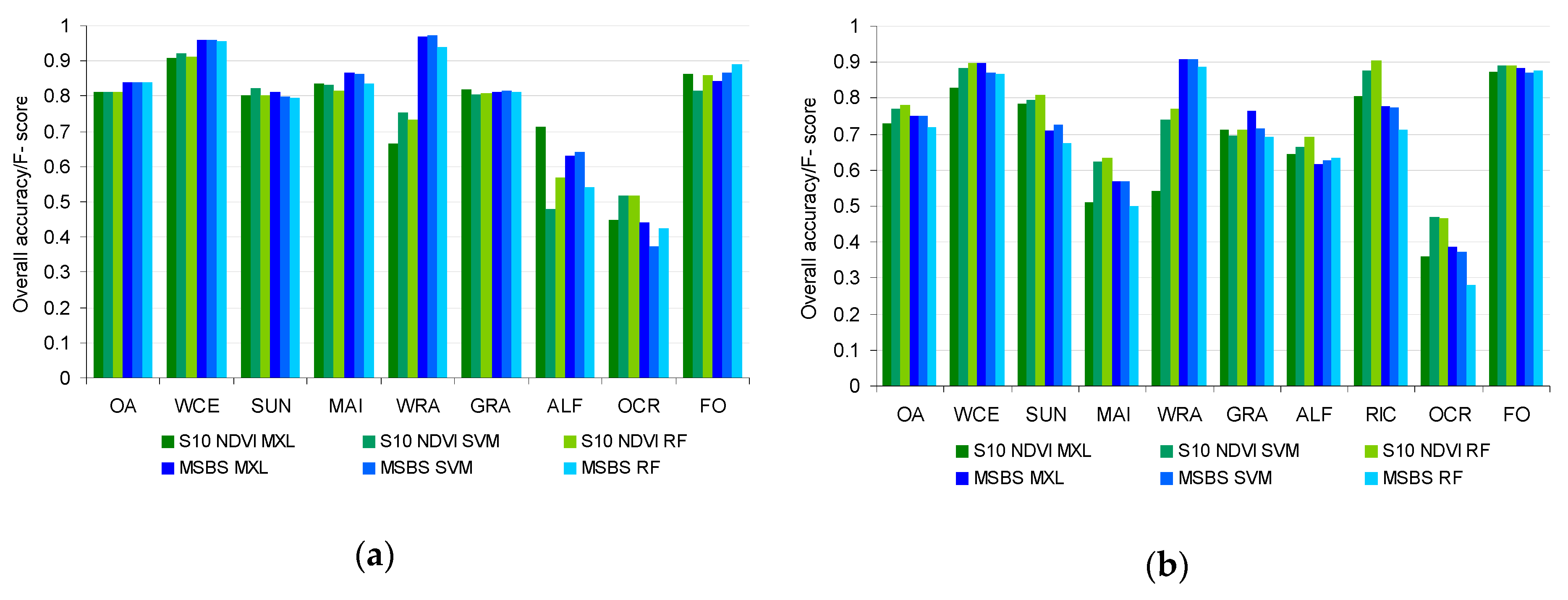
We compared the crop/land-use maps derived by two input Sentinel-2 datasets i.e., S10 NDVI time series and MSBS and the three classification methods. Figure 4 shows the overall map accuracy (OA) and the class F-scores for all compared maps, calculated using Equations (6) and (5) respectively. The broad-leaved forest and coniferous forest classes were combined for the purpose of the accuracy assessment into a single class forest. This was necessary because very few reference points of coniferous forest class were available. However, it was important to retain both forest types in the adopted legend and therefore the maps as they have quite different phenology.

The OA of the Sentinel-2-derived crop/land-use maps varied between 72% and 84%. The best OA for Knezha test site, which was 84%, was achieved with the MSBS dataset and the results were very similar for all three classification methods. The S10 NDVI dataset produced slightly less accurate classification results (OA = 81%), and again, without major discrepancy between the classification methods. In the Belozem test site, none of the maps reached the 80% OA threshold. The most accurate map (OA = 78%) was produced by RF classification using the S10 NDVI dataset as input.

The F-scores differed significantly between classes. The highest F-scores, overall, were achieved for winter cereals and forest, for which the accuracy levels of about 85%–95% were stable among input dataset, classification method and test site. The F-score for the winter rapeseed was also high (about 90%–95%), but only with the MSBS dataset. The accuracy of rice was also dependent on the dataset but here S10 NDVI provided more accurate results than MSBS, with F-score up to 90%. The maximum achieved F-score for sunflower was 81%–82% for the two test sites. For that class, the input using S10 NDVI dataset generated consistent results for all classifiers and test sites. This was not the case with MSBS used as the input dataset, which performed well only in the Knezha test site. The accuracies of classification varied for other classes depending on the test site. In general, it was lower for the Belozem test site. For example, the F-score of maize was above 80% in Knezha for all maps, while it was 63% at maximum in the Belozem test site. Not so severe but still an important discrepancy was observed for grasslands where F-scores were about 10% lower in the Belozem test site for most combinations of input datasets and the used classifiers. Finally, the class with lower F-scores was other crops, not higher than 52%.

When class F-scores and OA were considered there is no clear indication which of the two input image datasets was better. For some classes this may be the MSBS while for others the S10 NDVI. The decision also seemed to vary with the test site and the classification method which further complicate the comparison. In short, none of the Sentinel-2 datasets is perfect for all classes. One clear advantage of the MSBS classifications in both test sites was the markedly higher F-score for winter rapeseed. The S10 NDVI dataset, from the other hand, provided better results for rice when SVM or RF were used. The same was true also for other crops, but as stated earlier the accuracy for this class was very low in all maps.

The relative performance of the three classification methods, MXL, SVM, and RF, with the test site and image dataset being constant, can be most easily assessed using the OA (Figure 4). As stated before, the three methods performed equally well for the S10 NDVI dataset in the Knezha test site. There was no difference between methods for the MSBS dataset in the Knezha test site as well. For the S10 NDVI dataset in the Belozem test site RF produced the highest OA, followed by SVM and MXL. For the MSBS dataset in Belozem RF produced the lowest OA, while MXL and SVM topped the ranking with equal OAs (Figure 4). In any case, the differences between the classifiers were negligible in magnitude. Another approach to evaluate the performance of classifiers is presented in

Table 4. Number of classes for which MXL, SVM, and RF was the best performing method according to the F-scores (Figure 4). Note that the columns do not add up to 10 or 9 i.e., the numbers of classes in the Belozem and Knezha test site maps respectively (the mapped classes in Knezha test site are nine because there is no rice). This is because broad-leaved forest and coniferous forest classes were combined for the purpose of the accuracy assessment and because when more than one method performed best the class is counted to each of them.

Classification Method	S10 NDVI/Belozem	S10 NDVI/Knezha	MSBS/Belozem	MSBS/Knezha
MXL	1	4	7	5
SVM	2	5	3	4
RF	9	2	1	2

. The table contains the number of classes for which each of MXL, SVM, and RF was the best performing method according to the F-score (Figure 4). The data in the table shows for example that the RF classifier was top ranked in all nine classes (broad-leaved and coniferous forest being combined) in the Belozem test site map based on S10 NDVI. However, this classifier was worst for the other combinations of Sentinel-2 input image dataset and test site (Table 4). The SVM and MXL classifiers were more stable in their performance in terms of the number of classes for which they provided the highest F-score.

Finally, it is worth to single out, once again, that more accurate maps were produced in the Knezha test site regardless of the input dataset used or classifier. These results were consistent through all classes.

As a conclusion, we selected, for both test sites, the map derived by using the MSBS Sentinel-2 dataset and the SVM method as an optimal variant which was to be used as reference data for the sub-pixel PROBA-V classification. The MSBS-derived maps were preferred because of the higher accuracy for the winter rapeseed class. The SVM classifier was selected because it showed stable performance and, in general, allowed the use of a smaller training dataset than the MXL method.

3.2. Sub-Pixel Classification of NDVI Time Series from PROBA-V 100 m

Table 5. Results from the validation of the estimated AFIs: per pixel and after aggregation to the 80 artificial regions of 10x10 km². R², b, and m are the coefficient of determination, intercept and slope of the linear regression of true area fractions (%) on estimated area fractions (%). The column Relative area indicates the relative importance of each class for the total of both test sites according to the reference Sentinel-2 maps. ANN-artificial neural network; SVR-support vector regression. The last row shows the result of the regression performed with data from all pixels, regardless of their class.

Class		ANN						SVR
	Relative area (%)	Pixel			Region			Pixel			Region
		R2 (%)	b (%)	m	R2 (%)	b (%)	m	R2 (%)	b (%)	m	R2 (%)	b (%)	m
Winter cereals	27.9	73.7	5.82	1.00	86.8	4.56	0.95	73.4	7.27	1.07	85.8	6.87	0.97
Sunflower	16.1	64.9	3.41	0.98	84.2	1.60	1.02	65.2	4.34	1.03	81.1	3.01	1.04
Broad-leaved forest	15.6	70.2	1.62	0.97	87.6	−0.61	1.02	78.1	2.43	1.08	91.7	0.85	1.08
Maize	12.8	61.7	2.38	0.89	88.4	1.30	0.90	63.0	3.14	1.00	89.2	2.52	0.96
Grassland	12.6	36.1	3.59	0.78	65.2	1.43	0.88	46.8	2.86	1.10	67.4	2.69	1.01
Alfalfa	5.3	29.1	1.47	0.48	76.2	0.90	0.50	33.2	2.02	1.04	72.9	1.39	1.10
Other crops	3.9	35.5	0.79	0.64	75.1	−0.21	0.80	44.0	0.75	0.82	87.9	−0.07	0.98
Winter rapeseed	3.0	30.9	−0.10	0.46	39.1	−0.44	0.48	37.3	−0.58	0.68	30.6	0.19	0.49
Coniferous forest	2.0	34.2	−0.38	0.44	91.0	−1.53	0.63	54.8	−0.01	0.77	95.9	−0.22	0.78
Rice	0.8	38.5	−0.44	0.43	84.8	−0.84	0.52	69.1	−0.15	0.82	96.4	−0.22	0.81
All classes	-	57.8	1.33	0.86	84.7	−1.14	1.02	64.9	1.91	1.04	89.0	0.40	1.13

shows the validation results for the estimated AFIs at pixel level and at the level of the 80 artificial regions using the two methods. The overall R² amounted to 57.8% at pixel-level for the ANN, with higher scores for some of the dominant classes (73.7% for winter cereals, 64.9% for sunflower, 70.2% for broad-leaved forest and 61.7% for maize), but far worse performance for some other classes (e.g., 29.1% for alfalfa and 30.9% for winter rapeseed). The classes with higher R² also had a regression line with the slope close to one and intercept close to zero, which shows that the estimates were not biased. 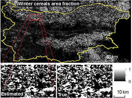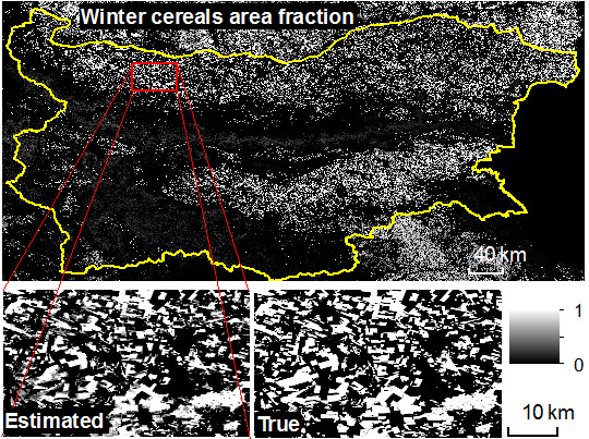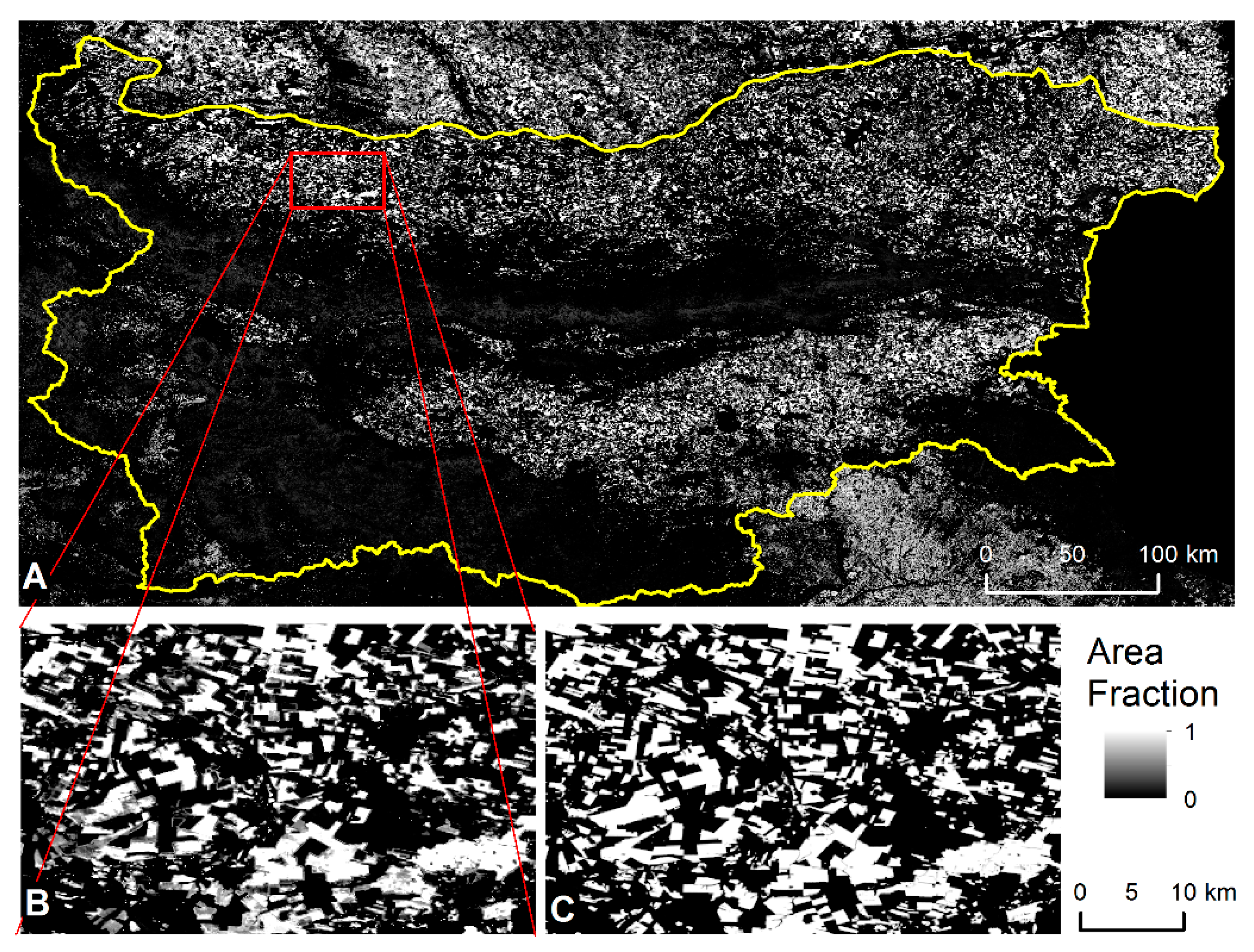Figure 5 and Figure 6 show the AFIs for winter cereals and winter rapeseed, which are one of the most accurately and one of the least accurately estimated classes respectively. The ANN was generally successful in representing the spatial distribution of winter cereals as indicated by the similar spatial patterns depicted in the estimated and the true winter cereals AFIs (Figure 5B,C). In contrast, the spatial distribution of winter rapeseed was poorly characterized by the estimated AFI (Figure 6B,C). This was due to widespread overestimation of the true area fraction for this class.

The overall R² amounted to 64.9% at pixel-level for the SVR, with highest scores for broad-leaved forest (78.1%) and winter cereals (73.4%). Again, alfalfa and winter rapeseed were the classes which performed poorly. For most classes, the R² was higher for SVR. ANN resulted in higher R² only for winter cereals, but the difference was negligible. The most pronounced difference between the two methods was observed for rice, for which R² increased by 31% when SVR was used instead of ANN. The two methods also differed in the slope of the regression line for the rarest and poorly performing classes; it was closer to 1 with the SVR (for example see alfalfa in Table 5).

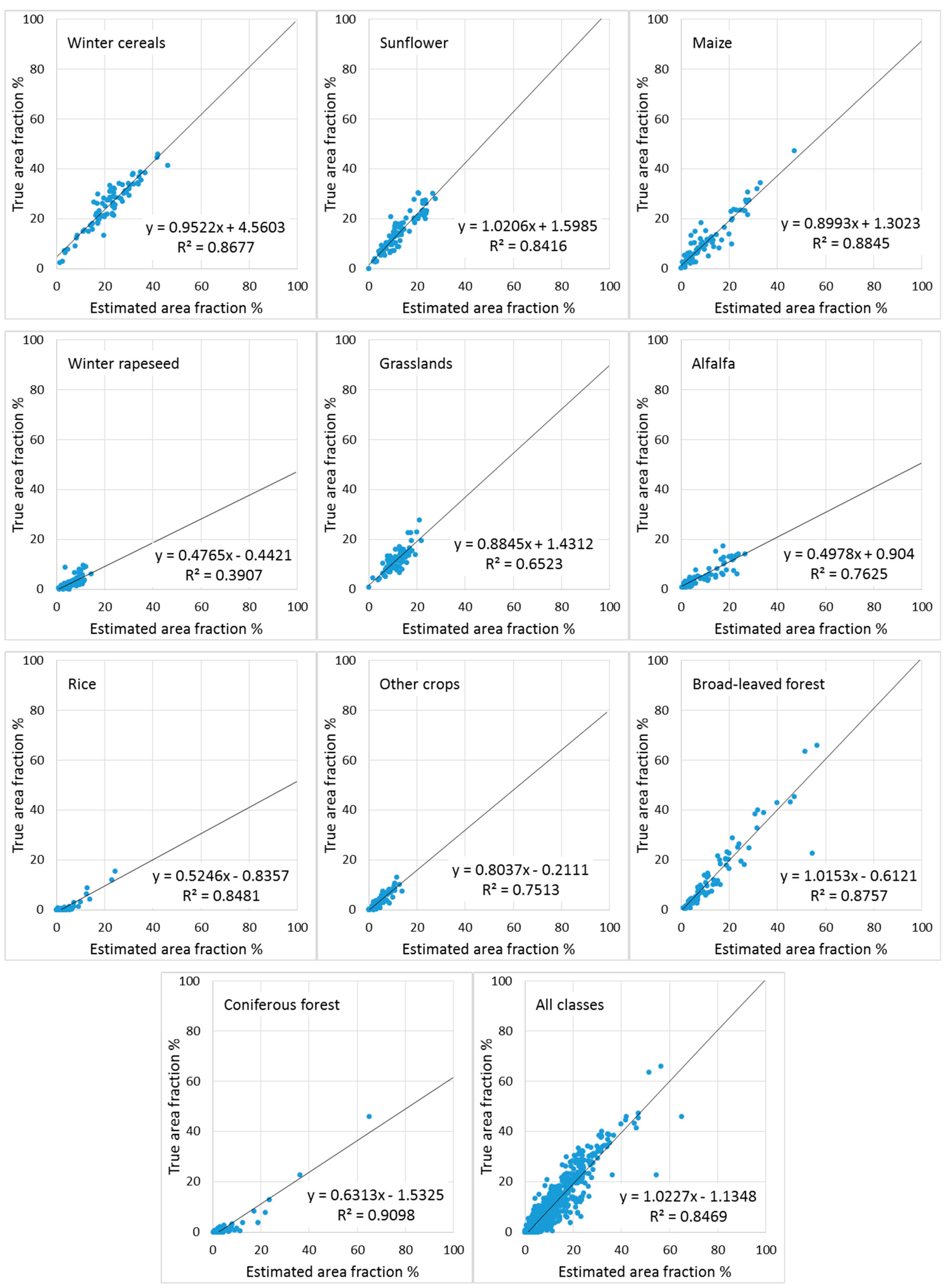
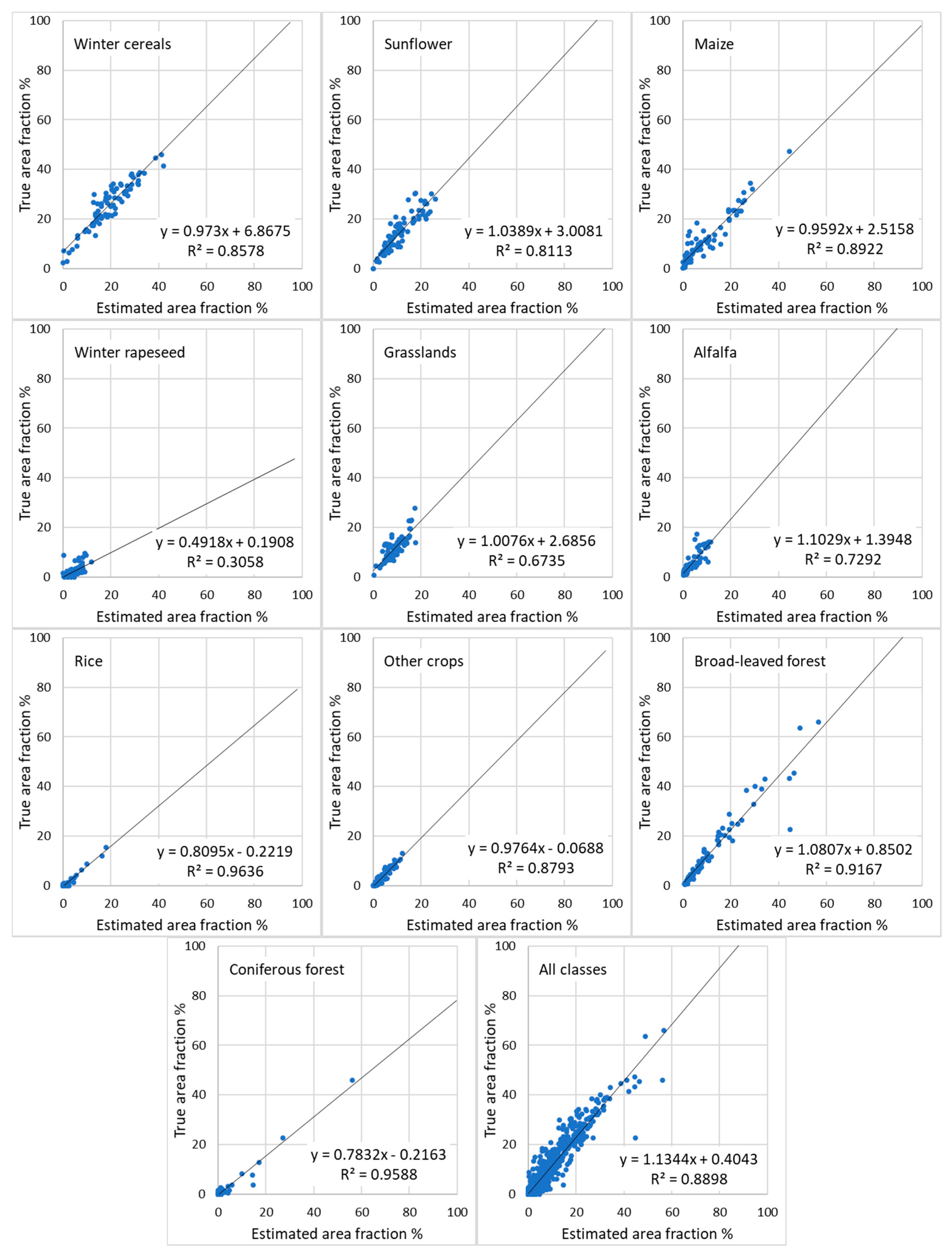
The regional aggregation drastically improved the AFI estimation accuracies (Table 5) for both methods. Figure 7 shows the scatterplots of estimated versus true area fractions for the ten classes and for the overall result (all classes merged together) at the region level obtained by ANN. Figure 8 shows the corresponding data for the SVR method. When all classes are considered together, the R² was raised from 57.8% per pixel to 84.7% per region for the ANN method (Table 5). The rise in the corresponding figures for the SVR method was from 64.9% to 89.0%. The improvement of R² was most important for the small classes: alfalfa, rice, other crops, and coniferous forest. With the ANN method the bias remained high in the estimates of alfalfa, coniferous forest, and rice, for which an overestimation of these true area fractions was observed (Table 5, Figure 7). With the SVR method the bias was much smaller for these same classes. Note, that severe overestimation was observed for winter rapeseed with both ANN and SVR, and this class did not show any practically important improvement in accuracy after regional aggregation.

4. Discussion

This study applied ANN and SVR methods for sub-pixel classification to produce crop (and land use) map of Bulgaria from PROBA-V 100 m NDVI time series. These methods were reported before using other low-resolution satellite images but have not been tested, to our knowledge, with PROBA-V 100 m data. Unlike previous studies (e.g., [1]), which made use of existing crop type databases for training of the sub-pixel classification, here, the aim was to test the feasibility of an approach which is independent of such datasets. For this aim, crop/land-use maps of two test sites derived by classification of Sentinel-2 data were first produced. The classifications were trained with a limited number of ground truth observations collected during the dedicated field campaigns. The resulted high-resolution maps (10 m) provided the reference data needed for training and validation of the PROBA-V 100 m sub-pixel classification. In this study we considered the results of the Sentinel-2 data classifications as reference or ground truth even though they were not 100% accurate. This is justified in the cases where better ground truth data was not available or was too onerous to acquire.

Even though this study demonstrated an approach for crop mapping at national level, which was independent of existing crop type datasets, such as IACS, it did require the additional effort of collecting ground truth data in a small number of representative test sites. In addition, if spatial differences in crops phenology or cropping density were observed, the region should be stratified on an agro-meteorological principal or other agronomic parameters and should separate PROBA-V classifications made in each sub-region [1].

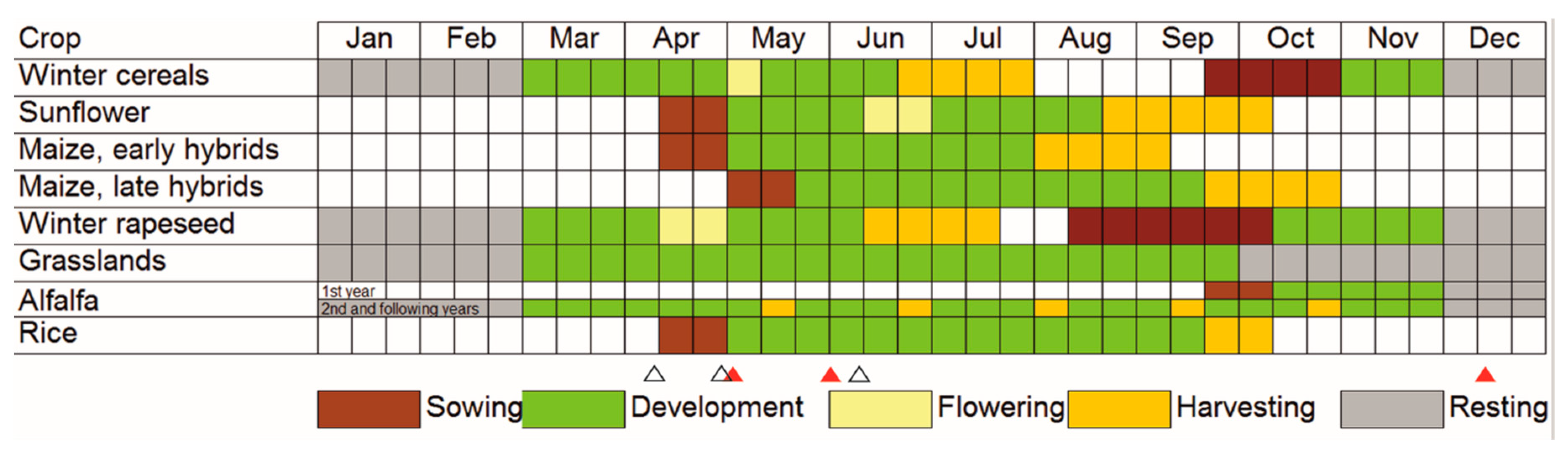
Two input datasets were compared for the production of reference, high-resolution crop maps from Sentinel-2 imagery. The approach using S10 NDVI time series as input data had the advantage of being operationally fully automated, and was generally less affected by the availability of cloud-free Sentinel-2 images. Disadvantage lay on the classification accuracy for the winter rapeseed class. The misclassification of winter rapeseed was not unexpected as the NDVI time profile of that crop was very similar to that of winter cereals. The approach using multidate stack of Sentinel-2 spectral bands (i.e., the MSBS approach) as input data had the advantage of enabling the extraction of more spectral information from a Sentinel-2 image including that of red edge bands. However, it highly relied on the availability of cloud-free images and their acquisition timing relative to important crop phenological events. The acquisition dates of the cloud-free Sentinel-2 images used for the multidate stack in this study seemed appropriate for most crops (at least in the Knezha test site) because they coincided with the periods when both winter and summer crops were observable in the field (Figure 3). Moreover, the MSBS approach was successful in discriminating between winter cereals and winter rapeseed. For instance, April–May is the period of flowering of winter rapeseed and is the best time for discriminating it from winter cereals. The better performance of using MSBS dataset as input for discriminating winter rapeseed indicated that the spectral characteristics induced by the flowering were better captured by the combined nine Sentinel-2 bands. It can be concluded here that crop classification using Sentinel-2 data may deliver maps with higher accuracy when individual spectral bands of the images registered on the phenologically important dates are used as input. In the circumstances of unavailability, or for operational purposes, the approach using NDVI time series may be preferable.

None of the three hard classifiers tested for the Sentinel-2 classifications i.e., MXL, SVM, and RF, guarantied markedly and consistently a higher accuracy of classification. For example, RF was clearly the most successful method in classifying the S10 NDVI dataset in the Belozem test site, but was outperformed by the other methods when applied to the MSBS dataset or to the Knezha test site. To conclude, as with the input image dataset, no general recommendation could be given as for a best classifier in any circumstances. Moreover, such generalization of results was neither possible nor sought in this study. Instead, our results suggested that different classifiers should be tested for crop mapping using Sentinel-2 imagery, according to the region of interest and the dataset available for the input.

The lower accuracy of the crop/land-use maps of the Belozem test site may be related to the quality of the input satellite data and factors specific to this site. First, the accuracies for the classifications based on the MSBS datasets may differ due to the input images with different registration dates for the two test sites. In particular, the Knezha MSBS dataset contained three images in the most important period from April to June, while the Belozem MSBS dataset contained only two, the third being from the winter period (12 December). The S10 NDVI datasets for both test sites was composed of a regular series of 10-day composites covering the same period. The two NDVI time series, however, cannot be regarded as of precisely the same quality because the availability of cloud-free observations has some effect on the smoothing algorithm [24]. The land-use or landscape specificity of each test site also contributed to the different accuracy. For example, the agricultural landscape in the Belozem test site was more complex due to the smaller average field size, greater diversity of cultivated crops, and larger relative area of the problematic other crops class.

Furthermore, the accuracy of the Sentinel-2-derived reference maps used for training of the PROBA-V classification is worth more discussion. For both test sites we selected the maps derived by SVM classification using the MSBS datasets. The OA of the maps was 75% and 84% for the Belozem and Knezha test site respectively. These accuracies may not seem high for a reference dataset especially when compared with ground-based crop datasets such as IACS available in many developed countries. However, maps derived from Sentinel-2 remain a feasible option as reference data where no other ground truth information is available, for example in data-poor countries. Compared with other studies the accuracy achieved here is reasonable. For example, Van Tricht et al. [40] applied random forest classification algorithm on monthly NDVI time series from Sentinel-2 to map 12 crops and land cover types in Belgium. An overall accuracy of 78% was obtained using an input dataset encompassing the period March–August and 72% using another dataset covering the period March–June. Better results were achieved by incorporating radar data from Sentinel-1. Vuolo et al. [27], also using random forest, classified multi-date Sentinel-2 datasets. They achieved overall accuracy of ~95% in mid-August based on stacks of five and eight cloud-free images in 2016 and 2017 growing seasons respectively. The accuracy was slightly lower (~85%) when images acquired till the end of June were used (four and six images in the two growing seasons respectively). In our study the number of used cloud-free images was lower, as such were not available, and this may explain the lower accuracy.

The MSBS dataset included 20 m Sentinel-2 bands upscaled to a higher spatial resolution of 10 m. The error introduced in the classifications by this upscaling was not thoroughly evaluated in this study. However, a preliminary test using the MXL classifier showed that the classification accuracies remain very similar when the datasets of 10 or 20 m resolution were used as input.

The area fraction estimates derived by applying the two sub-pixel classification methods on the PROBA-V time series were less reliable at pixel level, especially for small or less frequent classes. The SVM method slightly outperformed the ANN method. However, these results were better than those reported in the previous study by Verbeiren et al. [1], which used ANN, notably for main dominant classes. For instance, the two highest R² values reported by these authors were 64% (for the forest class) and 58% (for the winter wheat class). In this study, the maximal R² values obtained at pixel level with the ANN method were 74% (for winter cereals) and 70% (for broad-leaved forest).

Nevertheless, our results confirmed once again that the accuracy of the estimated area fractions increased with the aggregation per region. For our artificial regions of size 100 km², R² was over 80% for most classes with R² = 87% for the most important class (winter cereals) when the ANN method was applied. It can be expected that the accuracy may be further increased if estimates are aggregated at the municipality level, which most often, has areas larger than 100 km². The crop area estimates are usually reported at the level 3 of the Nomenclature of Territorial Units for Statistics (NUTS 3) in the European Union, which is even larger.

In this study the area fraction estimates derived by the SVR method were more accurate than those derived by ANN at both pixel and region-level, as far as the R² is considered. This remained true for most classes and for the general assessment of all classes combined.

The results of this work may be further considered in the context of future operational monitoring, for example on monthly basis, of the sub-pixel crop area fraction for whole country, based on 100 m imagery. Indeed, for classifying a large area using high resolution datasets, at high temporal frequency, would involve a large amount of ground truth data, and mosaicking dozen individual tile classification results. When only the crop area fractions at a certain administrative zone are needed, and its updates are frequently required, the sub-pixel classification as we described here would be the most convenient way.

5. Conclusions

This study showed that the sub-pixel classification approach, used previously with 1 km SPOT-VEGETATION and other low-resolution imagery to classify crop types, was applicable to PROBA-V 100 m data as well. The two used methods, ANN and SVR gave similar results with slightly better performance for the SVR. The obtained area fractions of major crop/land-use classes in Bulgaria had relatively low accuracy at pixel level (R² = 57.8% with the ANN method and 64.9% with the SVR method), but much better accuracy was observed with aggregation at an artificial region level of 100 km² (R² = 84.7% with the ANN method and 89.0% with the SVR method). In addition, we tested the hypothesis that a sub-pixel PROBA-V classification can be produced at national level when insufficient ground truth is available to train the sub-pixel classification directly. We showed that the usage of Sentinel-2 derived land-use maps is an appropriate approach for extrapolating the small ground truth dataset. For crop mapping applications, the well selected multidate Sentinel-2 individual bands were the most suitable input, at least for applications in that part of Europe. In an operational perspective, as the automation is entirely feasible, the use of NDVI time series as the input is recommended. Further studies should compare the performance of sub-pixel and hard classification approaches on PROBA-V 100 m data for the purpose of regional crop area estimation. Furthermore, the effect of the different size of agricultural parcels on the relative performance of sub-pixel and hard classification approaches should be investigated. In addition, further studies are needed to assess the performance of other machine learning algorithms for regression with the objective of crop area fraction estimation from PROBA-V 100 m data.

References

1. Verbeiren, S.; Eerens, H.; Piccard, I.; Bauwens, I.; Orshoven, J.V. Sub-pixel classification of SPOT-VEGETATION time series for the assessment of regional crop areas in Belgium. Int. J. Appl. Earth Obs. Geoinform. 2008, 10, 486–497. [Google Scholar] [CrossRef]
2. Bastin, L. Comparison of fuzzy c-means classification, linear mixture modelling and MLC probabilities as tools for unmixing coarse pixels. Int. J. Remote Sens. 1997, 18, 3629–3648. [Google Scholar] [CrossRef]
3. Hill, R.A.; Granica, K.; Smith, G.M.; Schardt, M. Representation of an alpine treeline ecotone in SPOT 5 HRG data. Remote Sens. Environ. 2007, 110, 458–467. [Google Scholar] [CrossRef]
4. Quarmby, N.A.; Townshend, J.R.G.; Settle, J.J.; White, K.H.; Milnes, M.; Hindle, T.L.; Silleos, N. Linear mixture modelling applied to AVHRR data for crop area estimation. Int. J. Remote Sens. 1992, 13, 415–425. [Google Scholar] [CrossRef]
5. Shao, Y.; Lunetta, R.S. Comparison of Sub-pixel Classification Approaches for Crop-specific Mapping. In Proceedings of the 2009 17th International Conference on Geoinformatics, Fairfax, VA, USA, 12–14 August 2009. [Google Scholar] [CrossRef]
6. Foody, G.M. A Fuzzy Sets Approach to the Representation of Vegetation Continua from Remotely Sensed Data: An Example from Lowland Heath. Photogramm. Eng. Remote Sens. 1992, 58, 221–225. [Google Scholar]
7. MacLachlan, A.; Roberts, G.; Biggs, E.; Boruff, B. Subpixel land-cover classification for improved urban area estimates using Landsat. Int. J. Remote Sens. 2017, 38, 5763–5792. [Google Scholar] [CrossRef]
8. Wu, K.; Du, Q.; Wang, Y.; Yang, Y. Supervised Sub-Pixel Mapping for Change Detection from Remotely Sensed Images with Different Resolutions. Remote Sens. 2017, 9, 284. [Google Scholar] [CrossRef]
9. Atkinson, P.M.; Cutler, M.E.J.; Lewis, H. Mapping sub-pixel proportional land cover with AVHRR imagery. Int. J. Remote Sens. 1997, 18, 917–935. [Google Scholar] [CrossRef]
10. Foody, G.M.; Lucas, R.M.; Curran, P.J.; Honzak, M. Nonlinear mixture modelling without end-members using an artificial neural network. Int. J. Remote Sens. 1997, 18, 937–953. [Google Scholar] [CrossRef]
11. Liu, W.; Wu, E.Y. Comparison of non-linear mixture models: Sub-pixel classification. Remote Sens. Environ. 2005, 94, 145–154. [Google Scholar] [CrossRef]
12. Foody, G.M.; Cox, D.P. Sub-pixel land cover composition estimation using a linear mixture model and fuzzy membership functions. Int. J. Remote Sens. 1994, 15, 619–631. [Google Scholar] [CrossRef]
13. Bovolo, F.; Bruzzone, L.; Carlin, L. Novel Technique for Subpixel Image Classification Based on Support Vector Machine. IEEE Trans. Image Process. 2010, 19, 2983–2999. [Google Scholar] [CrossRef] [PubMed]
14. Liu, Q.; Trinder, J.; Turner, I. A comparison of sub-pixel mapping, methods for coastal areas. ISPRS Ann. Photogramm. Remote Sens. Spat. Inf. Sci. 2016, 3, 67–74. [Google Scholar] [CrossRef]
15. Heremans, S.; Van Orshoven, J. Machine learning methods for sub-pixel land-cover classification in the spatially heterogeneous region of Flanders (Belgium): A multi-criteria comparison. Int. J. Remote Sens. 2015, 36, 2934–2962. [Google Scholar] [CrossRef]
16. Dierckx, W.; Sterckx, S.; Benhadj, I.; Livens, S.; Duhoux, G.; Van Achteren, T.; Francois, M.; Mellab, K.; Saint, G. PROBA-V mission for global vegetation monitoring: Standard products and image quality. Int. J. Remote Sens. 2014, 35, 2589–2614. [Google Scholar] [CrossRef]
17. Toté, C.; Swinnen, E.; Sterckx, S.; Adriaensen, S.; Benhadj, I.; Iordache, M.-D.; Bertels, L.; Kirches, G.; Stelzer, K.; Dierckx, W.; et al. Evaluation of PROBA-V Collection 1: Refined Radiometry, Geometry, and Cloud Screening. Remote Sens. 2018, 10, 1375. [Google Scholar] [CrossRef]
18. Lambert, M.; Waldner, F.; Defourny, P. Cropland Mapping over Sahelian and Sudanian Agrosystems: A Knowledge-Based Approach Using PROBA-V Time Series at 100-m. Remote Sens. 2016, 8, 232. [Google Scholar] [CrossRef]
19. Zhang, X.; Zhang, M.; Zheng, Y.; Wu, B. Crop Mapping Using PROBA-V Time Series Data at the Yucheng and Hongxing Farm in China. Remote Sens. 2016, 8, 915. [Google Scholar] [CrossRef]
20. Durgun, Y.Ö.; Gobin, A.; Van De Kerchove, R.; Tychon, B. Crop Area Mapping Using 100-m Proba-V Time Series. Remote Sens. 2016, 8, 585. [Google Scholar] [CrossRef]
21. Czaplewski, R.L. Accuracy assessment of maps of forest condition—Statistical design and methodological considerations. In Remote Sensing of Forest Environments: Concepts and Case Studies; Wulder, M., Franklin, S., Eds.; Kluwer Academic Publishers: Norwell, MA, USA, 2003; pp. 115–142. [Google Scholar]
22. Hay, A.M. Sampling designs to test land-use map accuracy. Photogramm. Eng. Remote Sens. 1979, 45, 529–533. [Google Scholar]
23. Viovy, N.; Arino, O.; Belward, A. The Best Index Slope Extraction (BISE): A method for reducing noise in NDVI timeseries. Int. J. Remote Sens. 1992, 13, 1585–1590. [Google Scholar] [CrossRef]
24. Swets, D.L.; Reed, B.C.; Rowland, J.D.; Marko, S.E. A weighted least-squares approach to temporal NDVI smoothing. In Proceedings of the ASPRS Annual Conference, Portland, OR, USA, 17–21 May 1999; American Society for Photogrammetry and Remote Sensing: Bethesda, MD, USA, 1999; pp. 526–536. [Google Scholar]
25. Savitzky, A.; Golay, M.J.E. Smoothing and Differentiation of Data by Simplified Least-Squares Procedures. Anal. Chem. 1964, 36, 1627–1639. [Google Scholar] [CrossRef]
26. Eerens, H.; Haesen, D.; Rembold, F.; Urbano, F.; Tote, C.; Bydekerke, L. Image time series processing for agriculture monitoring. Environ. Model. Softw. 2014, 53, 154–162. [Google Scholar] [CrossRef]
27. Vuolo, F.; Neuwirth, M.; Immitzer, M.; Atzberger, C.; Ng, W. How much does multi-temporal Sentinel-2 data improve crop type classification? Int. J. Appl. Earth Obs. Geoinform. 2018, 72, 122–130. [Google Scholar] [CrossRef]
28. Wolters, E.; Dierckx, W.; Iordache, M.; Swinnen, E. PROBA-V Products User Manual v3.01; VITO: Mol, Belgium, 2018; p. 110. Available online: proba-v.vgt.vito.be/sites/default/files/Product_User_Manual.pdf (accessed on 20 December 2018).
29. Vapnik, V.N. The Nature of Statistical Learning Theory; Springer: New York, NY, USA, 1995. [Google Scholar]
30. Huang, C.; Davis, L.S.; Townshend, J.R.G. An assessment of support vector machines for land cover classification. Int. J. Remote Sens. 2002, 23, 725–749. [Google Scholar] [CrossRef]
31. Mountrakis, G.; IM, J.; Ogole, C. Support vector machines in remote sensing: A review. ISPRS J. Photogramm. Remote Sens. 2011, 66, 247–259. [Google Scholar] [CrossRef]
32. Lary, D.J.; Alavi, A.H.; Gandomi, A.H.; Walker, A.L. Machine learning in geosciences and remote sensing. Geosci. Front. 2016, 7, 3–10. [Google Scholar] [CrossRef] [Green Version]
33. Breiman, L. Random forest. Mach. Learn. 2001, 45, 5–32. [Google Scholar] [CrossRef]
34. Belgiu, M.; Drăguţ, L. Random forest in remote sensing: A review of applications and future directions. ISPRS J. Photogramm. Remote Sens. 2016, 114, 24–31. [Google Scholar] [CrossRef]
35. van der Linden, S.; Rabe, A.; Held, M.; Jakimow, B.; Leitão, P.J.; Okujeni, A.; Schwieder, M.; Suess, S.; Hostert, P. The EnMAP-Box—A Toolbox and Application Programming Interface for EnMAP Data Processing. Remote Sens. 2015, 7, 11249–11266. [Google Scholar] [CrossRef]
36. Pedregosa, F.; Varoquaux, G.; Gramfort, A.; Michel, V.; Thirion, B.; Grisel, O.; Blondel, M.; Prettenhofer, P.; Weiss, R.; Dubourg, V.; et al. Scikit-learn: Machine Learning in Python. J. Mach. Learn. Res. 2011, 12, 2825–2830. [Google Scholar]
37. Wang, J.; Neskovis, P.; Cooper, L.N. Training Data Selection for Support Vector Machines. In Proceedings of the Advances in Natural Computation: First International Conference, ICNC 2005, Changsha, China, 27–29 August 2005; Wang, L., Chen, K., Ong, Y.S., Eds.; Lecture Notes in Computer Science. Springer: Berlin/Heidelberg, Germany, 2005; Volume 3610, pp. 554–564. [Google Scholar] [CrossRef]
38. Olofsson, P.; Foody, G.M.; Stehman, S.V.; Woodcock, C.E. Making better use of accuracy data in land change studies: Estimating accuracy and area and quantifying uncertainty using stratified estimation. Remote Sens. Environ. 2013, 129, 122–131. [Google Scholar] [CrossRef]
39. Labatut, V.; Cherifi, H. Accuracy Measures for the Comparison of Classifiers. In Proceedings of the 5th International Conference on Information Technology, Amman, Jordan, 11–13 May 2011; Al-Zaytoonah University of Jordan: Amman, Jordan, 2011; pp. 1–5. [Google Scholar]
40. Van Tricht, K.; Gobin, A.; Gilliams, S.; Piccard, I. Synergistic Use of Radar Sentinel-1 and Optical Sentinel-2 Imagery for Crop Mapping: A Case Study for Belgium. Remote Sens. 2018, 10, 1642. [Google Scholar] [CrossRef]
Figure 1. Location of the two test sites with available reference data in Bulgaria (Knezha to the north and Belozem to the south). The borders of the administrative units at Nomenclature of Territorial Units for Statistics level 3 are shown as well as the arable land (source: Corine Land Cover) and the corresponding Sentinel-2 tiles. Each test site was divided in artificial regions 10 × 10 km2 for validation purposes (see the text for explanation).
Remotesensing 11 01370 g001
Figure 2. Relative area of the main crops and crop types in the two test sites according to the Integrated Administration and Control System (IACS) 2018 dataset. Crops and crop types are abbreviated as follows: WCE—winter cereals, SUN—sunflower, MAI—maize, WRA—winter rapeseed, GRA—grasslands, ALF—alfalfa, RIC—rice, and OCR—other crops. Note that, IACS do not cover all agricultural land; in particular, grasslands and permanent crops are not fully covered.
Remotesensing 11 01370 g002
Figure 3. Crop calendar of the main crops and crop types in the study areas. The approximate time of the Sentinel-2 images used for the multi-date classification (see Section 2.2) are indicated by open triangles (Knezha) and red triangles (Belozem).
Remotesensing 11 01370 g003
Figure 4. Overall accuracy (OA) and F-score per class for the crop/land-use maps of “Knezha” (a) and “Belozem” (b) test sites derived by different types of Sentinel-2 data (i.e., S10 NDVI time series and MSBS) and different classification method: MXL—maximum likelihood, SVM—support vector machine, and RF—random forest. Classes are abbreviated as follows: WCE—winter cereals, SUN—sunflower, MAI—maize, WRA—winter rapeseed, GRA—grasslands, ALF—alfalfa, RIC—rice, OCR—other crops, and FO—broad-leaved and coniferous forest combined.
Remotesensing 11 01370 g004
Figure 5. (A) Estimated area fraction image for the winter cereals class derived by the artificial neural network (ANN) sub-pixel classification of PROBA-V 100 m normalized difference vegetation index (NDVI) time series over Bulgaria. (B) Excerpt from the image in (A) for part of “Knezha” test site. (C) True area fraction image for the same region as (B) derived from the reference Sentinel-2 classification.
Remotesensing 11 01370 g005
Figure 6. (A) Estimated area fraction image for the winter rapeseed class derived by ANN sub-pixel classification of PROBA-V 100 m NDVI time series over Bulgaria. (B) Excerpt from the image in (A) for part of “Knezha” test site. (C) True area fraction image for the same region as (B) derived from the reference Sentinel-2 classification.
Remotesensing 11 01370 g006
Figure 7. Scatterplots showing the correspondence between true and ANN estimated area fractions at regional level. The dots represent the averages for the artificial 10 × 10 km2 regions as depicted in Figure 1. N = 80, except for the scatterplot for “All classes”, where N = 800.
Remotesensing 11 01370 g007
Figure 8. Scatterplots showing the correspondence between true and support vector regression (SVR) estimated area fractions at regional level. The dots represent the averages for the artificial 10 × 10 km2 regions as depicted in Figure 1. N = 80, except for the scatterplot for “All classes”, where N = 800.
Remotesensing 11 01370 g008