TopoLAP: Topology Recovery for Building Reconstruction by Deducing the Relationships between Linear and Planar Primitives

Abstract

Limited by the noise, missing data and varying sampling density of the point clouds, planar primitives are prone to be lost during plane segmentation, leading to topology errors when reconstructing complex building models. In this paper, a pipeline to recover the broken topology of planar primitives (TopoLAP) is proposed to reconstruct level of details 3 (LoD3) models. Firstly, planar primitives are segmented from the incomplete point clouds and feature lines are detected both from point clouds and images. Secondly, the structural contours of each plane segment are reconstructed by subset selection from intersections of these feature lines. Subsequently, missing planes are recovered by plane deduction according to the relationships between linear and planar primitives. Finally, the manifold and watertight polyhedral building models are reconstructed based on the optimized PolyFit framework. Experimental results demonstrate that the proposed pipeline can handle partial incomplete point clouds and reconstruct the LoD3 models of complex buildings automatically. A comparative analysis indicates that the proposed method performs better to preserve sharp edges and achieves a higher fitness and correction rate than rooftop-based modeling and the original PolyFit algorithm.

1. Introduction

Three-dimensional building models, as the dominant type of man-made object in urban scenes, play an important role in the foundation of the smart city. Applications including immersive visualization, city planning, and navigation, etc. [1] impose a high demand to both the topology and texture information of the building models, the automatic reconstruction of which remains a long-standing challenge. The technical problems and state-of-the-art solutions have been thoroughly discussed and depicted in a rich body of literature [2,3,4].

Since points of the façades suffer from missing data caused by glass materials, occlusion, and scanning angle limitation, etc., most of the mature solutions resort to LoD2 [5] models which only focus on the rooftop modeling for the past decades. The ISPRS test project on urban classification and 3D building reconstruction gives a comprehensive conclusion towards rooftop modeling from point clouds and/or images [6]. Among the common strategies, the data-driven methods highly depend on the data quality, while the model-driven methods are confined to certain building types. Modeling without the façade points not only reduces the level of details but also leaves the generalized boundaries of roofs inaccurate without the constraint of adjacent façades.

Proliferation in the fields of laser scanning and imaging sensors enable the point clouds, either acquired from light detection and ranging (LiDAR) or photogrammetry, to describe large-area 3D scenes efficiently, providing a good data foundation for building reconstruction with a higher level of detail. LiDAR point clouds with high density and precision, along with the high-resolution images taken at the same time can be obtained, cutting-edge researches involve the fusion of point clouds and image data for extra reliable information [7,8]. The façade point clouds can be utilized to assist the boundary generation with sharp features preserved and automatic LoD3 modeling is now conceivable. However, high redundancy, partial missing and poor distribution, especially alongside the boundary of the buildings in the urban scenes are still common obstacles for modeling complex buildings [9]. Even if the point clouds are dense enough, it is nearly impossible to preserve all the details of small planes and ignore the noise parts at the same time by plane segmentation only from point clouds (Figure 1). It is imperative to synthetically utilize the characteristics of the multi-source data and to take the data deficiency into account during the reconstruction process.

To address these challenges, special emphasis is placed on the structural contour extraction and topology recovery in order to deal with the incomplete planar primitives involved in building reconstruction. The main contributions of this paper consist of:

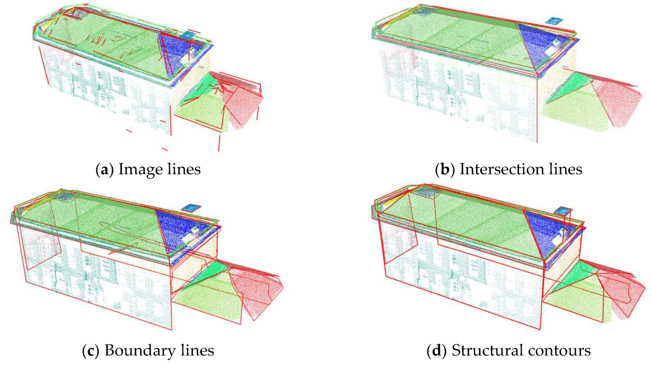
• Structural contour extraction from point clouds, taking full advantages of the characteristics of topological and textural information.
• Topology recovery for the incomplete planar primitives based on the relationship between the linear and planar primitives, which generates a complete set of candidate planes to describe the building.
• An optimized pipeline to reconstruct polyhedral models efficiently with high fitness to point clouds and high correctness of planar primitives.

The rest of this paper is organized as follows. After a brief survey on related work given in Section 2, an overview of our approach is expressed in Section 3. Subsequently, detailed algorithms of the proposed method are explained in Section 4 and Section 5. The experiments are carried out and discussed in Section 6. Finally, the conclusion is given in Section 7 drawn from the experimental results and the comparative analysis.

2. Related Works

In a common pipeline of primitive-based building reconstruction, planar primitives are segmented from the point clouds and the contours of each plane are extracted to deduce the adjacent relations. Ridges are intersected by the roof planes while the outward borders or boundaries of isolated planes are determined by contour generalization. The literature review of related research is given, focused on these key technologies including linear and planar primitive-based building reconstruction and the topology recovery towards an incomplete dataset.

2.1. Linear Primitive Extraction and Generalization

As linear primitives are salient in man-made objects, several studies extract line features to abstract the urban scenes. Methods based on images detect segments from images and isolated 3D lines can be triangulated from the matched 2D segment pairs [10,11]. Other methods resort to point clouds including the off-the-shelf algorithm RANSAC [12,13] to detect shapes of known parameters. Apart from the line fitting algorithm, another essential research is to extract the line alignment for 2D or 3D point cloud. Outstanding research has involved a contrario detection theory [14,15,16], which can be further applied to find the boundary of a plane. Hackel et al. combine the classification and contour extraction to extract topologically meaningful object contours [17].

Another researched topic aims at polygon generalization in order to extract the boundary of buildings. Some methods detect contours of rooftops from unstructured point clouds [18,19]. Wang et al. uses structural linear features to regularize the mesh of buildings based on images, which is susceptible to data deficiency [20]. Either extracting rooftops or footprints from point clouds [21] or detecting building areas from images based on deep learning [22], the precision of the final model relies on the polygon generalization. However, the generalization algorithms are vulnerable to the quality of the point clouds and the topology of rooftops is hard to recover only from the boundaries, which involves a bunch of manual interference to obtain qualified models.

2.2. Planar Primitive-Based Building Reconstruction

Scholars assume that the buildings are formed by planes and describe the building by a regular arrangement of planes [23,24,25]. Considering that the regularization of the planar parameters is directly dependent on the results of the initial extraction, several methods perform plane segmentation and plane regularization simultaneously in order to generate more complete planar primitives [26,27]. In [28], Holzmann et al. selects tetrahedral from 3D Delaunay triangulation and generates plane-constrained surfaces. Based on the Manhattan-World assumption [29] that most planes of the buildings are axis-aligned, algorithms refine the planar parameters on hard constraints [30,31] in large-scale indoor or outdoor scenes.

To recover the topology information of the planar primitives and finally reconstruct the vector building models, roof topology graph (RTG)-based methods are proposed to reconstruct the LoD2 model [32,33,34], which ignore the façades. As for the LoD3 building reconstruction, the cutting edge algorithm PolyFit [35] casts the reconstruction as a binary labeling problem to select optimal candidate faces from planar primitives. Compared to RTG-based methods, PolyFit is not subject to local topologies. However, it creates spurious artifacts and fails at missing data [28] since manifold and watertight are specifically required.

2.3. Topology Repair towards the Incomplete Dataset

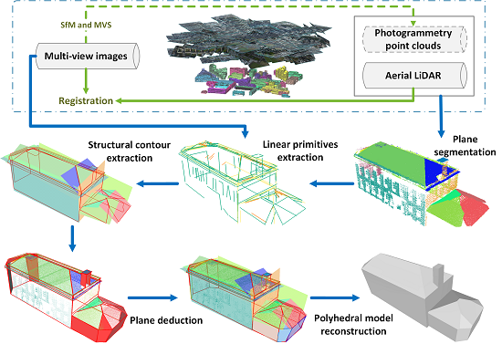
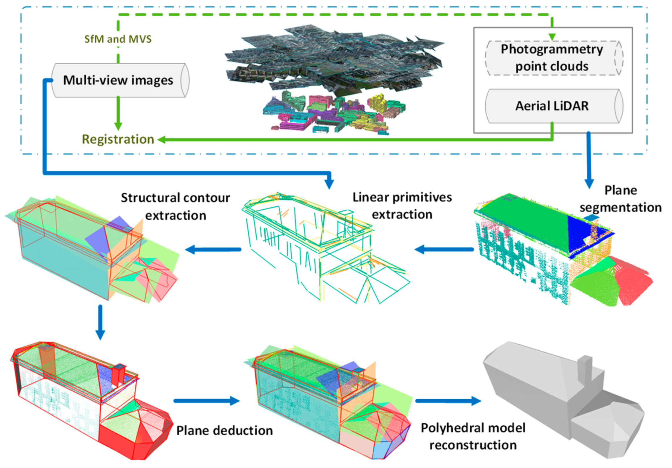
When dealing with the building of complex structures, planar primitives are susceptible to be corrupted by the unscalable segmentation, small walls, and varying accuracy. Research that falls into this category aims to deal with the incomplete primitives. Zolanvari et al. detects the opening area after plane segmentation [36]. Towards the RTG, a graph edit dictionary is designed to correct the graph as a graph-to-graph problem but is limited by the known entries already in the dictionary [37]. More flexible strategies divide the building into several components, each of which is reconstructed by RTG [38]. However, these methods heavily depend on the point-based segmentation results and only handle the data of rooftops. The Manhattan-Modeler retrieves the façade using the height map, which can only be used to repair vertical walls [39]. Other methods involve ground data aimed at façade modeling, which introduces extra data cost [40,41,42,43].

3. Overview

The input data of our method include point clouds and the corresponding multi-view images. Point clouds can be obtained by multi-view stereo (MVS) or laser scanning (registration of LiDAR and optic images is required). Ground filtering and building segmentation are conducted as preprocessing. Assuming that the point cloud $\mathcal{P}$ of a single building and image sequence $ℐ$ with ground sample distance $Gs{d}_{ℐ}$ are given, the average spacing of $\mathcal{P}$ is calculated as ${\mathrm{Av}}_{\mathcal{P}}$ based on 9 nearest neighbor points. Planar primitives are firstly segmented from point clouds based on RANSAC [13] with a distance threshold ${\epsilon }_d$. We assume that plane primitives $\left\{{\mathrm{\Omega }}_i\in \mathrm{\Omega }\right\}$ are detected from $\mathcal{P}$, each equipped with a set of points $\mathcal{P}$_Ωi and Distance({p|p ∈ $\mathcal{P}$_Ωi}, Ω_i) < ε_d, which constraints the thickness of the plane.

The proposed pipeline consists of two main parts: structural contour extraction and topology recovery by plane deduction. To recover the missing planes which break the topology for building reconstruction, the accurate and structural linear features are needed for implication. Common contour extraction methods enclose the planar points and generate complete profiles, taking the cost of the low geometric precision and missing topology information. Thus, the structural contour extraction procedure is addressed and conducted before the plane deduction. The whole pipeline of our method is as follows and displayed in Figure 2.

(1) Structural contour extraction. We extract the contours of each planar primitive segmented from the original point clouds. Due to varying noise, missing data and low density, especially in the façades, it is difficult to snap accurate sharp outlines using common boundary generalization methods towards rooftop or footprint. With the auxiliary of topology information of adjacent planes and image data, we extract intersection lines and image lines, as well as boundary lines from point clouds, and then generate candidates by intersection. Contours are selected from the candidates which enclose the planar primitive. Structural linear features are preserved while scattered parts are ignored to provide reliable hints for plane detection.

(2) Topology recovery by plane detection. Based on the extracted structural contours and feature lines, the hypothesis of missing planes is generated by a plane detection strategy and then evaluated based on the topological relationships between the lines and the existing planar primitives. The structural contours are extracted for the newly validated line groups subsequently. Then, an iteration procedure is conducted to excavate all the possible planar hypothesis and linear primitives to retrieve a complete set of planar primitives. Finally, planar primitives are assembled to generate over-complete face candidates for binary labeling-based building reconstruction framework. Invalid candidates are eliminated according to the minimum 2D distance to the corresponding original plane before the energy function solution.

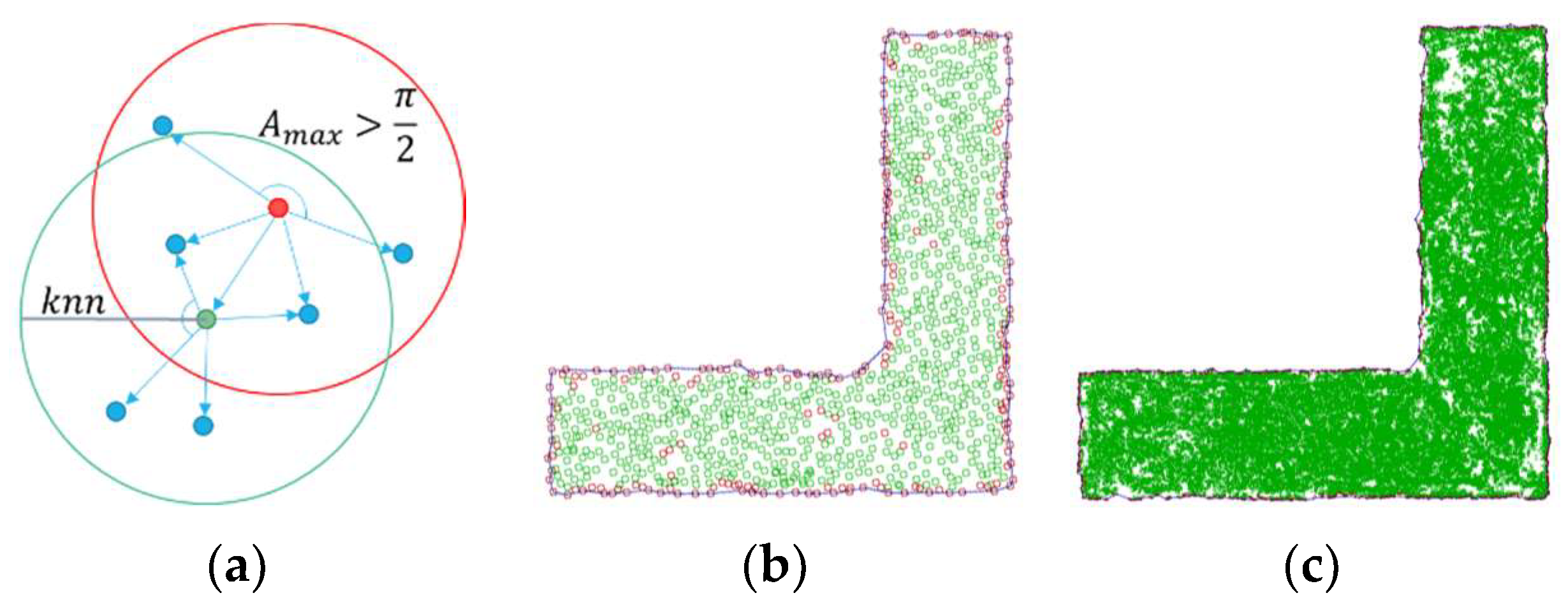
4. Structural Planar Contour Extraction

Given the initial plane primitives $\left\{{\mathrm{\Omega }}_i\in \mathrm{\Omega }\right\}$, the concave hull of each plane is calculated by alpha shape with the alpha value ${\epsilon }_{\alpha }$. If more than one component generated, split the plane until each plane contains only one connected component enclosed by ${\epsilon }_{\alpha }$ concave hull.

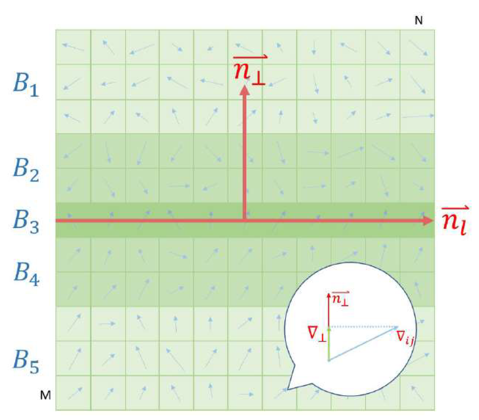
4.1. Linear Feature Detection

Three types of linear features are extracted from point clouds or images. Each type can be a complete or partial description of the outline respectively while each has its own advantageous and disadvantageous characteristics (Figure 3).

(1) Image lines. 2D line segments extracted from each image are matched between overlapped images and then triangulated to reconstruct 3D lines. We use the strategy proposed and implemented by Hofer et al. [10], which can abstract the scene but with some errors and interruption. Although topologically poor and incomplete, image lines are of high texture sharpness and high geometric precision, which implies that the lines align to the sharp edges in images and can be a crucial compensation if the point cloud is severely impaired.

(2) Intersection lines. Each plane primitives are intersected with all other planes to obtain the intersection lines. Notably, the intersection is valid only if it is overlapped by the convex hull of two intersected planes. Threshold ${\epsilon }_{ints}$ is used to constrain the maximum distance from the convex hull segments to the intersection line. Further, the end point of the intersection segment is determined by the interception of the projection of the convex hull. Intersection lines serve as the most robust topology hint for adjacent relations of planes. However, intersection lines are incomplete if some of the walls are missing and abundant erroneous relations may occur due to the non-adaptive snapping tolerance [44].

(3) Boundary lines. A point is marked as a boundary point if the maximal angle between the point and two neighboring points within the 16 nearest neighbors is larger than a certain angle ($\frac{\pi }{2}$ by default) (Figure 4). Then, boundary lines are detected from boundary points based on RANSAC. To ensure the boundary lines sketch the plane completely, the consecutive strings of outline segments from the concave hull are used to link the interrupted boundary line. Refer to Algorithm 1 for the pseudo-code of the procedure. However, the connected boundary lines enclose the plane points, but the geometric precision is low and structural information is weak due to the scattered character of the boundary points.

Algorithm 1. Boundary line contouring
Input: Concave hull point string ${\mathit{S}}_{\mathit{C}}$;     Boundary lines ${\mathit{S}}_{\mathit{l}\mathit{i}\mathit{n}\mathit{e}}$ and the endpoints ${\mathit{S}}_{\mathit{e}\mathit{n}\mathit{d}}$
Output: Looped boundary line strings ${\mathit{L}}_{\mathit{b}\mathit{d}\mathit{r}\mathit{y}}$;
1 for each $pt\in S_C$ do
2	if $pt\notin S_{line}$ then
3		Status($pt$) = UNUSED
4	end
5 end   6 for each $p{t}_1\in S_{end}$ do
7   8   9	$p{t}_2\in S_{end}$ closest to $p{t}_1$  $p{t}_s\in S_C,p{t}_e\in S_C$ closest to $p{t}_1,p{t}_2$  for each $p{t}_s<pt<p{t}_e,$ Status($pt$) = UNUSED, $pt\in S_C$ do
10		add $pt$ to the final endpoint set $S_{add}$
11 12	end  for each $p{t}_i\in S_{add}$ do
13 14		$l_{new}=\left\{p{t}_i,p{t}_{i+1}\right\}$   add $l_{new}$ to $L_{bdry}$
15	end
16 end

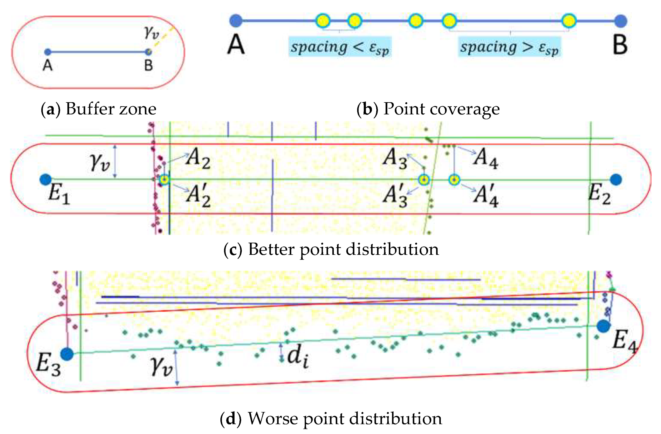
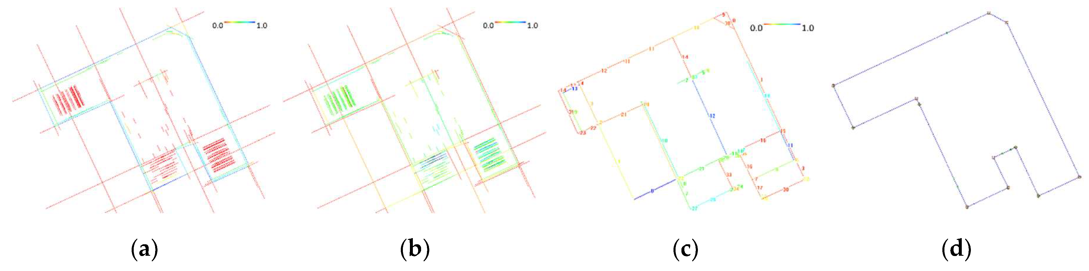
4.2. Contour Optimization

The topology completeness may be preserved taking the cost of geometry precision or vice versa in common boundary normalization strategies. To find a solution with a good trade-off between quality and compactness, we resort to integer linear programming [45] to select the optimal edges out of the over-complete set of the outline candidates composed of a loop string of boundary lines $L_{bdry}$, image lines $L_{image}$ and intersection lines $L_{ints}$ extracted previously.

4.2.1. Hypothesis Generation

The feature lines are intersected with each other to get the basic hypothesis. Each hypothesis is a sub-segment of the original feature line, which forms the candidate segments. For each plane, edges of the outline are selected from $N_{ℒ}$ candidate segments, denoted as:

$$ℒ=\{L_B,L_T,L_I|L_B\subset L_{bdry},L_T\subset L_{ints},L_I\subset L_{image}\}$$

(1)

where $L_B={\left\{l_b\right\}}_{b=1}^{N_B}$, $L_T={\left\{l_t\right\}}_{t=1}^{N_T}$, and $L_I={\left\{l_i\right\}}_{i=1}^{N_I}$ represents the boundary lines, intersection lines and image lines respectively.

We require the candidate segments to fit the edge with a balance of boundary point coverage in point clouds and the sharpness in images, and to “smoothly” form the outline, namely with constrained model complexity. The energy function is formed by a data term and a smooth term:

$$E\left(ℒ\right)=E_{data}\left(ℒ,ℬ,ℐ\right)+{\lambda }_s{E}_{smooth}\left(ℒ,\mathcal{V}\right)$$

(2)

where $ℬ$, $ℐ$, and $\mathcal{V}$ represents the boundary points in the plane, the images to which the plane can be projected, and the end points of the candidate edges, respectively. ${\lambda }_s$ is a scalar parameter to balance between data fitting and model complexity. Then the edge selection conundrum is cast as a binary linear problem of minimization of the weighted energy terms with certain constraints. $E^{*}=\underset{\chi }{min}E\left(ℒ\right)$ is solved based on graph cuts [46].

4.2.2. Energy Formulation

The fitting quality of the candidate can be evaluated from the aspect of point clouds (object-term) and the aspect of images (image-term). The data term is formulated as:

$$E_{data}=-{\displaystyle \sum }_{l\in ℒ}{x}_l\cdot \left(f\left(l\right)+{\lambda }_{pi}g\left(l\right)\right)$$

(3)

where $x_l$ indicates whether line $l$ is selected, i.e., 1 for selected and 0 for abandoned. $f\left(l\right)$ and $g\left(l\right)$ is the function of fitting quality of point distribution and texture sharpness, respectively. The scalar weighting factor ${\lambda }_{pi}$ balanced between two sub-terms is determined according to the ratio of ${\mathrm{Av}}_{\mathcal{P}}$ and $Gs{d}_{ℐ}$.

(1) Point distribution. The first part of the data term manifests the candidate’s fitting quality to the boundary points. For each candidate segment, a buffer zone with a radius ${\gamma }_v$ is given as displayed in Figure 5a. Then, the point distribution can be calculated based on the boundary points inside the buffer zone from the measurement of mean distance and point coverage.

$$f(l)=(1-\frac{1}{{\gamma }_v}\cdot \frac{{{\displaystyle \sum }}_{p\in Z_l}Dist\left(p,l\right)}{N_{\left\{p\right|p\in Z_l\}}})\cdot Cov\left(l\right)$$

(4)

$$\left\{p\right|p\in Z_l\}=\{p\in ℬ|D_{\perp }\left(p,l\right)<{\gamma }_v\}$$

(5)

$$Dist\left(p,l\right)=min\left\{D_{\perp }\left(p,l\right),D\left(p,l_e\right)\right\}$$

(6)

where $Z_l$ represents the buffer zone of $l$ and $Dist\left(p,l\right)$ measures the point-to-segment distance. $N_{\left\{p\right|p\in Z_l\}}$ counts the number of boundary points in $Z_l$.

$$Cov\left(l\right)=\frac{1}{\left|l\right|}\cdot {\displaystyle \sum }_{D\left(p_i,p_j\right)<{\epsilon }_{sp}}D\left(p_i,p_j\right)$$

(7)

where $p_i$ and $p_j$ are the adjacent points projected on $l$. $\left|l\right|$ measures the length of $l$. Both the distance aspect and the coverage aspect are valued between 0 and 1. The object-term decreases when boundary points fall in the buffer zone with a smaller distance to the line and better coverage rate. Figure 5c,d give an example for a good distribution and a relatively worse one respectively.

(2) Texture sharpness. To make sure the outline is fit to the actual boundary as captured in the image, the sharpness of each candidate line in related images is involved in this image-term. As mentioned in LSD [47], the line segments are validated by the number of level-line aligned pixels in a line-support region. A binary descriptor, derived from the concept of Line Descriptor with Gradually Changing Bands (LDGCB) [48,49], is introduced to evaluate the gradient distribution in the line-support region, which is a rectangle composed of several bands extending on either side of the segment.

For each segment projected in the image, sharpness is calculated and expressed by a band gradient matrix (BGM) in the line-support region as illustrated in Figure 6. Assuming the line passes through $N$ pixels, the $BGM$ at $i^{th}$ pixel is formulated as:

$$BG{M}_i={\displaystyle \sum }_{j=1}^M{\omega }_j·\frac{{\nabla }_{ij}\cdot \overrightarrow{n_{\perp }}}{{\overrightarrow{n_{\perp }}}^2}\cdot \overrightarrow{n_{\perp }}$$

(8)

$${\omega }_j=\{\begin{array}{cc}0.7& j\subset B3\\ 0.2& j\subset B2{{\displaystyle \bigcup }}^{}B4\\ 0.1& j\subset B1{{\displaystyle \bigcup }}^{}B5\end{array}$$

(9)

where ${\nabla }_{ij}$ calculates the gradient at pixel $\left(i,j\right)$. $\overrightarrow{n_{\perp }}$ is the normal vector of line $l$. The number of bands is set to 5 in this study, with the widths of 3, 2, 1, 2, 3 respectively and $M=11$ accordingly. ${\omega }_j$ is the weighting coefficient for each band and is set to 0.7, 0.2, and 0.1 from close to far, quantized from the Gaussian function provided by LDGCB. Then the image-term can be formulated as the mean sharpness in projected images:

$$Sharp\left(l\right)=\frac{1}{t}{\displaystyle \sum }_{I_m\in {ℐ}_l^t}\frac{1}{N}{\displaystyle \sum }_{i=1}^N\parallel BG{M}_i\left({\mathrm{\Gamma }}_m\left(l\right)\right){\parallel }_2$$

(10)

$$g\left(l\right)=max(1,\frac{1}{{\epsilon }_g}Sharp\left(l\right))$$

(11)

where ${\mathrm{\Gamma }}_m$ projects a candidate line to the image $I_m$. Considering the camera’s geometric distortion, the view angle to each line is calculated according to the camera’s altitude. Among images onto which $l$ is projected, only $t$ images ${ℐ}_l^t$ with biggest view-angle are taken into consideration to make sure the candidate line, if selected, takes the eligible image view as during the texture mapping. $t$ is set to 5 if available. ${\epsilon }_g$ is empirically set to 30 as the maximal magnitude of the gradient component relative to the image quality, and the sharp is truncated by 1 to make the image-item value between 0 and 1.

(3) Model complexity. The end point is connected to four candidate edges if it is the intersection point of two feature lines, otherwise, it connects to only one candidate edge. The end point is marked as selected if and only if two of the connected lines are selected (2-link). Then the model complexity is validated based on whether the connected lines come from the same original feature line. To avoid over-fitting, the smooth term is designed as:

$$E_{smooth}=\frac{1}{N_{\mathcal{V}}}{\displaystyle \sum }_{v\in \mathcal{V}}[\Im \left(l_i^v\right)\ne \Im (l_j^v)]$$

(12)

where $N_{\mathcal{V}}$ is the number of endpoints; $\mathcal{V}$, $l^v$ represents the line connected to vertex $v$, and $\Im \left(l\right)$ maps candidate $l$ to its original feature line, and $[\cdot ]$ is the Iverson bracket, which equals to 0 if the two connected edges share the same feature line or 1 otherwise.

The effect of the candidates rendered by data-term and the optimization solution is illustrated in Figure 7. After solving the energy minimization function formulated in Equation (2), the generalized contour of the plane is extracted composed of a set of piecewise line segments. The contours extracted in this section abandoned tiny detailed boundary segments in order to preserve the structural line features as much as possible, which provides crucial implication for the plane deduction in the next step.

5. Plane Deduction Based on the Relationships between Linear and Planar Primitives

Plane segmentation and contour extraction in the last section only preserve plane segments with good distribution and ignore small faces in case of error-disturbance, which ensures the survived planes are stable and robust enough for topology reasoning. In this section, we discuss the characteristics of geometry primitives and elucidate the plane deduction strategies, retrieving a complete set of plane segments for polyhedral model reconstruction.

5.1. Geometry Primitive Candidates

Each plane primitive is equipped with the original segmented points and the optimized contour lines. In addition, intersection lines and image lines which are discarded by the contour optimization but lie inside the contour are kept and assigned to each plane, while the rest primitives remain unassigned, including scattered points and part of image lines. Then the geometry primitive candidates, i.e., planes candidate ${\mathcal{C}}_{\mathrm{\Omega }}$, lines candidate ${\mathcal{C}}_{ℒ}$, and points candidate ${\mathcal{C}}_{\mathcal{P}}$, are formed and expressed as follows:

$$\begin{gathered} {\mathcal{C}}_{\mathrm{\Omega }}=\left\{{\mathrm{\Omega }}_1,{\mathrm{\Omega }}_2,\dots ,{\mathrm{\Omega }}_n\right\} \\ {\mathcal{C}}_{ℒ}=\left\{{ℒ}_{{\mathrm{\Omega }}_1},{ℒ}_{{\mathrm{\Omega }}_2},\dots ,{ℒ}_{{\mathrm{\Omega }}_n},{ℒ}_{UA}\right\} \\ {\mathcal{C}}_{\mathcal{P}}=\left\{{\mathcal{P}}_{{\mathrm{\Omega }}_1},{\mathcal{P}}_{{\mathrm{\Omega }}_2},\dots ,{\mathcal{P}}_{{\mathrm{\Omega }}_n},{\mathcal{P}}_{UA}\right\} \end{gathered}$$

(13)

where $n$ represents the number of planes currently. The subscript index of $ℒ$ and $\mathcal{P}$ represents the plane that the primitive belongs to, and $UA$ for unassigned primitives. We denote this index attribute as assignment attribute ($Ass$).

For the sake of clarity, linear primitives are divided into four categories according to their relative position attribute to candidate planes and other line segments: border line (lines of the plane contour), crease line (a border line is marked as crease if it is overlapped with another Border Line from different planes, i.e., an intersection line), inner edge (lines assigned to a plane but not a border or a crease line), and needle line (unassigned lines).

5.2. Plane Detection from Lines and Validation Criterion

5.2.1. Line-and-Plane (LaP) Group

Generally, the RANSAC-based shape detection algorithm forms the basic shape hypothesis from points. However, scenes such as poor texture in MVS point clouds or façades uncovered by LiDAR scans invalidate the point-based detection, especially in the urban environment [28]. Given Lines Candidate ${\mathcal{C}}_{ℒ}$, RANSAC-based plane detection is redesigned using line segments as seed elements to detect potential planes which cannot be segmented by original point clouds. The consensus set requires at least two segments samples which satisfies that these segments are coplanar, and they are unassigned needle lines or belong to different planes, i.e., for the seed set of the $k$-$th$ RANSAC iteration ${\mathcal{S}}_k\subset {\mathcal{C}}_{ℒ}$:

$$\forall l_i,l_j\in {\mathcal{S}}_k:s.t.\{\begin{array}{c}Ass\left(l_i\right)=UA{\displaystyle \cup }Ass\left(l_j\right)=UA{\displaystyle \cup }Ass\left(l_i\right)\ne Ass\left(l_j\right)\\ \left(\overrightarrow{n_{l_i}}\times \overrightarrow{n_{l_j}}\right)\cdot \left(\overrightarrow{P{l}_{s_i}}-\overrightarrow{P{l}_{s_j}}\right)<{\epsilon }_{zero}\end{array}$$

(14)

where $l$ is represented by the start point and end point, $l=\left(P{l}_s,P{l}_e\right)$. $\overrightarrow{n_l}$ is the normal of $l$. ${\epsilon }_{zero}$ constrains the thickness tolerance of the plane model.

After iterated sampling, line-and-plane groups are generated, each of which contains at least two segments nevertheless many of them may be erroneous at this stage.

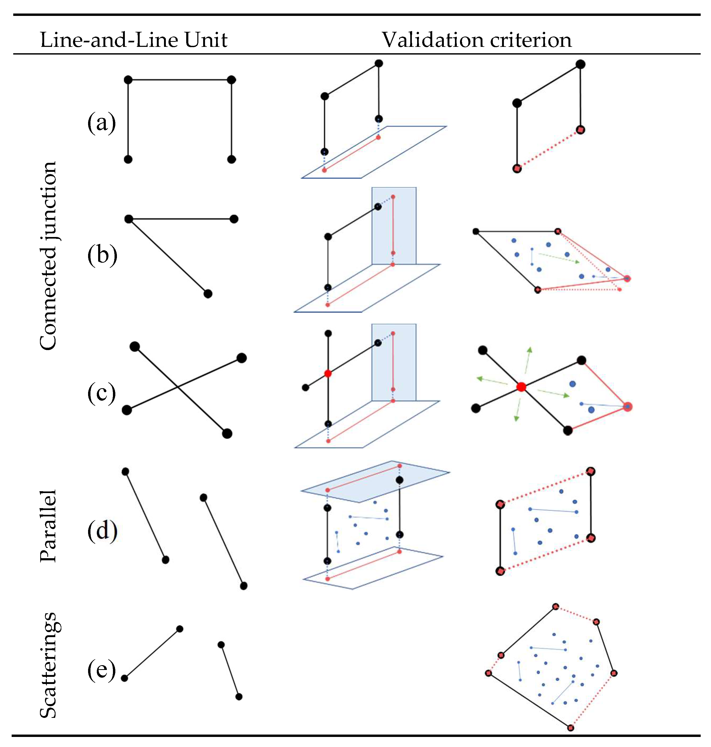
5.2.2. Line-and-Line (LaL) Unit

In each LaP group, relations of each segment are analyzed including connectivity, parallelism, and relative position attribute. Firstly, the convex hull of each plane is calculated and candidate lines closest to each convex hull segment are marked as Border Lines while the rest as Inner edges. Secondly, check if the border lines are connected or parallel otherwise and divide the LaL units into three categories: connected junction including three sub-classes, parallel pair, and scattered lines. In Figure 8 an example is displayed and the judgment is conducted successively from (a) to (e) as illustrated in Figure 9.

• Connected junction. Border Lines are considered as connected and snapped together if they satisfy that two lines intersect, and the sum of the distance from the intersection point to the closer end point of each segment is less than a distance threshold. (a) If three or more border lines are connected as a triple junction, check if the extended line of the outward borders meets an existing plane candidate. Connect the intersection points on the plane if found, otherwise, connect the two outward endpoints of the triple junction as the contour to enclose the unit. (b) If only two border lines connected, check if there are planes intersect with the junction. Take the connections of intersection points as contour segments if planes are found. If no plane is around (refer to the third subfigure in Figure 9b), find inner edges from ${ℒ}_{UA}$ and points from $\mathcal{P}$_UA inside the angle between the two segments. When more than $N_{sup}$ candidates are found, close the group polygon by convex hull; otherwise, add parallel segments to ${\mathcal{C}}_{ℒ}$ but leave this LaP group pending in the candidate pools. (c) For the junction that the segments are intersected but the endpoints are not connected, interrupt the segments by the intersection point and divide the group into 4 areas, each of which forms as the type (b). Examine each sub-part as (b) and confirm that with the largest sum of candidates the final LaP group.
• Parallel pair. Border lines that are confirmed as parallel pair are valid only if more than $N_{sup}$ candidates can be attached to the LaP. Then the borders are connected similarly to the triple junction as illustrated in Figure 9a.
• Scattering lines. LaP group where no connected junction or parallel pair can be detected is treated as a group of scattering lines (Figure 9e) and is validated simply by the number of lines and points attached to it, i.e., abandon the group to which less than $N_{sup}$ candidates can be attached.

This greedy strategy detects line-and-plane groups from all the candidates globally and then validate line-and-line units on the group at the local circumstance, which tends to excavate potential planes as complete as possible and ensure that only valuable planes adopted.

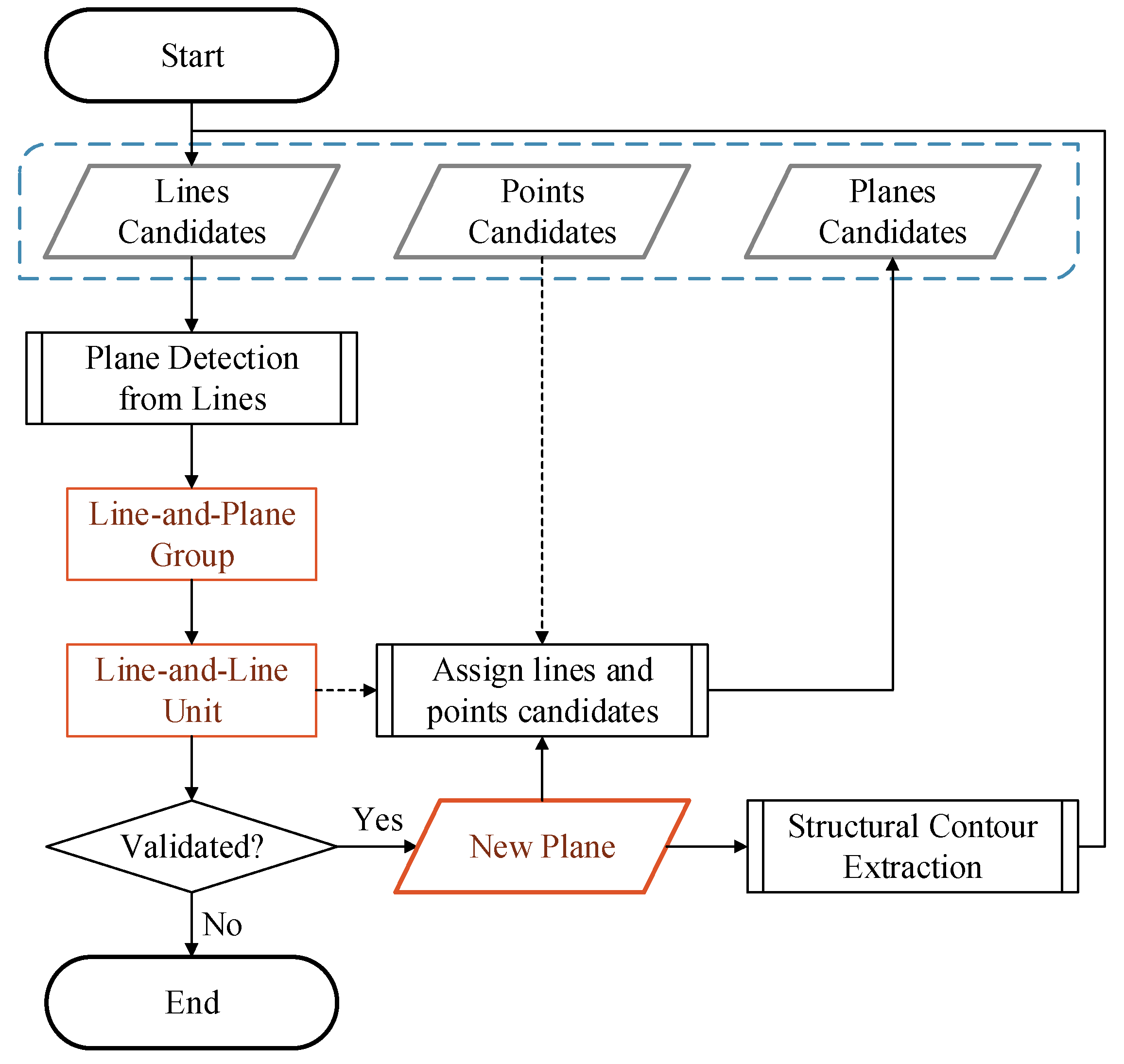
5.3. Deduction Iterations

The complete routine of the plane deduction is explained in this section, and the workflow is given in Figure 10. And an example of the deduction iteration is illustrated in Figure 11 Take candidates ${\mathcal{C}}_{\mathrm{\Omega }}$, ${\mathcal{C}}_{ℒ}$, and ${\mathcal{C}}_{\mathcal{P}}$ as input, the deduction strategy involves an iteration procedure as following steps:

• Planes are detected from ${\mathcal{C}}_{ℒ}$ based on RANSAC and new LaP groups $\left\{{\mathrm{LaP}}_i=\left({\mathrm{\Omega }}_i^{new},{ℒ}_{{\mathrm{\Omega }}_i^{new}}\right)\right\}$ are formed.
• For each ${\mathrm{LaP}}_i$, the LaL Unit is identified and evaluated according to each unit pattern. Once the LaL Unit is validated, assemble the lines of ${ℒ}_{{\mathrm{\Omega }}_i^{new}}$ as a new plane ${\mathrm{\Omega }}_i^{new}$ and assign lines and points candidates that are ${\mathsf{\epsilon }}_d$-close to this plane, retrieving from ${ℒ}_{UA}$ and ${\mathcal{P}}_{UA}$ respectively, to ${\mathrm{\Omega }}_i^{new}$.
• Subsequently, the structural contour of the plane ${\mathrm{\Omega }}_i^{new}$ is extracted based on the algorithm proposed in Section 4 and the contour segments are added into ${\mathcal{C}}_{ℒ}$ if available.
• Back to start and repeat steps 1–3. The next iteration starts with the increased ${\mathcal{C}}_{ℒ}$ until no more LaP group can be detected and/or no more LaL units can be validated.

To recover the missing planes as complete as possible, a few erroneous planes may be generated by the deduction although validation criterion gives strong constraints. However, the erroneous deduced plane hardly contains intensive points or lines candidates, thus can be discarded during the polygon model reconstruction, which will be expatiated in the next section.

5.4. Watertight Polyhedral Model Reconstruction based on Optimized PolyFit

In [35], Nan and Wonka proposed a framework to reconstruct the polygonal surfaces from point clouds as a binary labeling problem, which generates a reasonably large set of face candidates by intersecting plane primitives and then select an optimal subset from the candidates. The main problems that restraint its applicability in complex urban scenes are the missing data and the large amount of the candidates to be selected. The original PolyFit intersects all the planes as infinitely extending planes in the case of topology holes, which generates an avalanche of redundant candidate faces.

After plane detection, we have already repaired the topology of the buildings, which can be used as planar primitives to reconstruct the watertight polyhedral model. In addition, with the complete set of planar primitives and the optimized contours, we can eliminate the facets which are obviously invalid, which minimizes the amount hypothesis to improve efficiency and robustness. Each planar primitive is intersected by all other planes and is split into pieces of facets as the candidate faces. We assume that the candidate face is invalid if the minimal distance from the boundary of the face to the boundary of the original plane is larger than ${\epsilon }_{ints}$, which is the same threshold we used to generate intersection lines. Figure 12 shows an example to eliminate invalid candidates. Note that the enclosed boundary generated in Section 4.1 and the structural contour optimized in Section 4.2 are merged as the boundary of the original plane on the account of the completeness requirement at this stage.

6. Experimental Results and Discussion

6.1. Data Overview

Several real-world buildings from three different test areas with varying completeness levels, densities, and complexity are selected to evaluate our approach. Since our methods dedicate to reconstructing LoD3 models, dense LiDAR point clouds captured at low altitude are preferred. We use the Dublin datasets provided by Urban Modelling Group, University College Dublin, Ireland [50]. The MVS point clouds generated by MVE [51], and a set of sparse LiDAR point clouds captured at a rather high altitude in Ningbo, China are used for robustness test. The initial RANSAC-based plane segmentation results are taken as input data since plane segmentation is outside the scope of this study. We counted the planes manually as ground truths just for reference. Considering the high complexity of the building structures and the lack of standard, tiny planes smaller than 2 m² and subsidiary parts are ignored when counting ground truths of planar primitives. The input data and reconstructed models are displayed in

Table 1. Data overview and modeling results.

	Input Planar Segments	Reference Image	Output Models
Dublin1
Dublin2
Dublin3
Dublin4
Ningbo
MVS

and the properties are listed in

Table 2. Data properties and quantitative statistics.

Bld.	Input Data			Model Reconstruction
	#Points/av. Spacing 1	#Images/H/Gsd 2	#Planes/#Segments 3	#Deduced/#Model Planes 4	Runtime (s)
Dublin1	1.1M/0.11	115/300/3.4	103/65	125/109		35.5
Dublin2	695K/0.09	118/300/3.4	26/19	30/22		20.3
Dublin3	266K/0.07	41/300/3.4	23/14	29/25		25.6
Dublin4	158K/0.11	49/300/3.4	24/26	35/16		18.8
Ningbo	17K/0.64	99/900/4.8	15/14	25/14		15.9
MVS	237K/0.24	50/300/3.8	20/10	28/23		23.6

¹ The average spacing of the point clouds (m). ² The number of images in which the building is visible, the surveying altitude (m), and the ground sampling distance (cm). ³ The number of planes of ground truth and the input plane segments.⁴ The number of deducted planes and the planes of the final model.

Buildings in Dublin are of good point distribution but some of the planes are lost due to noise and segmentation scale; the façades of glass material are missing in the MVS point clouds; the building in Ningbo is partially covered by laser scanners and some of the planes are incorrectly segmented.

The settings of the key parameters involved in the proposed algorithms are listed in

Table 3. Parameter settings and representation.

Parameter	Value			Representation
	Dublin	Ningbo	MVS
${\epsilon }_d$	0.1 m	1 m	1 m	Distance threshold in plane segmentation
$se{g}_{pts}$	1000	200	1000	Min points number to support a plane segment
${\epsilon }_{\alpha }$	$2{\mathrm{Av}}_{\mathcal{P}}$			Max square of circumradius of facets in α-shape mesh
${\epsilon }_{ints}$	2m			Max distance to intersect two planes
${\gamma }_v$	0.5 m	2 m	2 m	Buffer threshold to support a line
${\lambda }_s$	10			Smooth scalar in contour optimization
$N_{sup}$	5			The min number of the sum of lines and points to support a new LaP group.

. ${\epsilon }_d$ and $se{g}_{pts}$ are used in plane segmentation, which is set according to the geometric precision and density of the point clouds. The buffer threshold ${\gamma }_v$ mainly matters the level of details of the building model, which is referred to decide how close two adjacent lines can be connected, and the area of the supporting zone of a line candidate during the contour optimization. The scalar parameters involved in PolyFit are set as ${\lambda }_f=0.46,{\lambda }_c=0.27,{\lambda }_m=0.27$ to resolve the linear program.

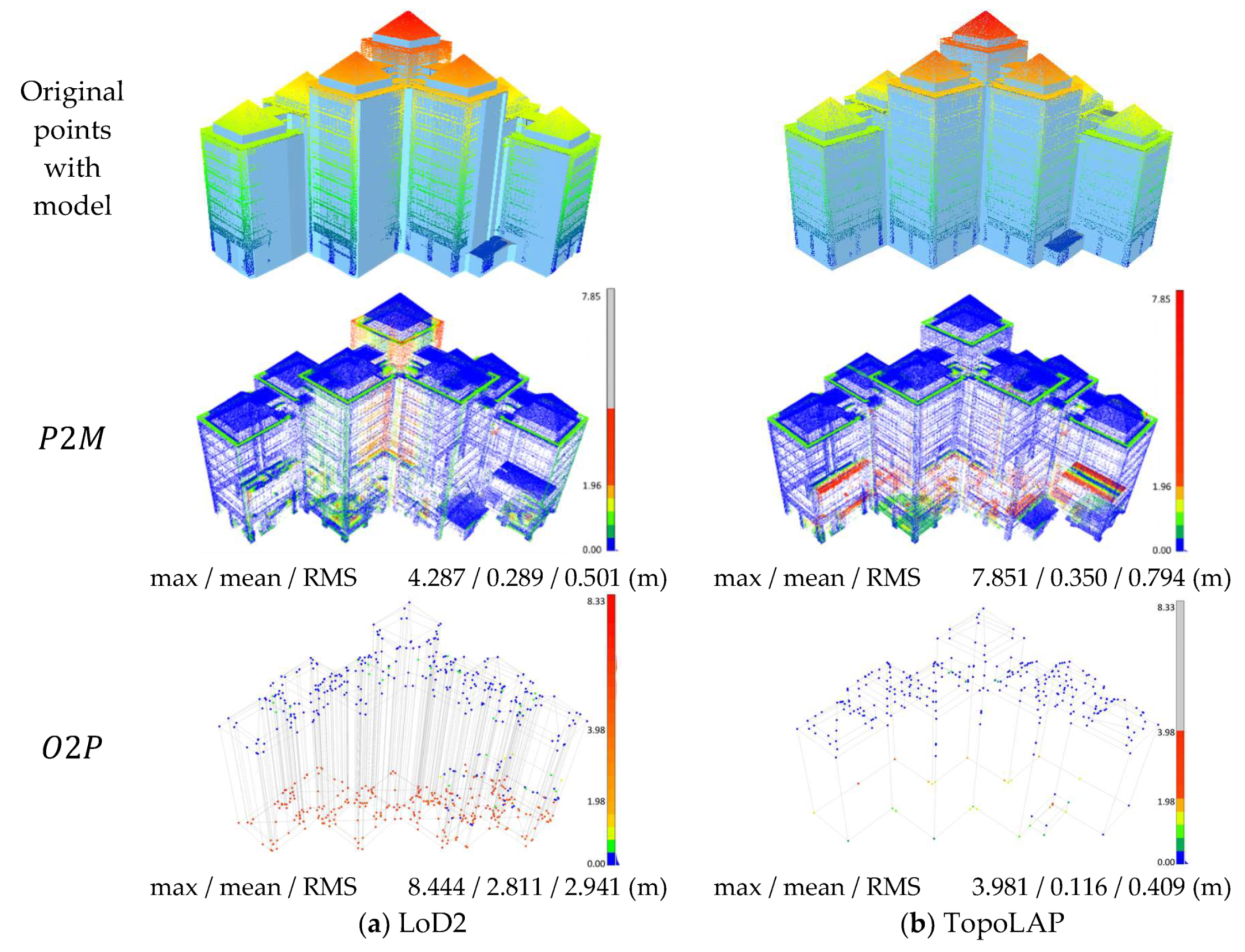
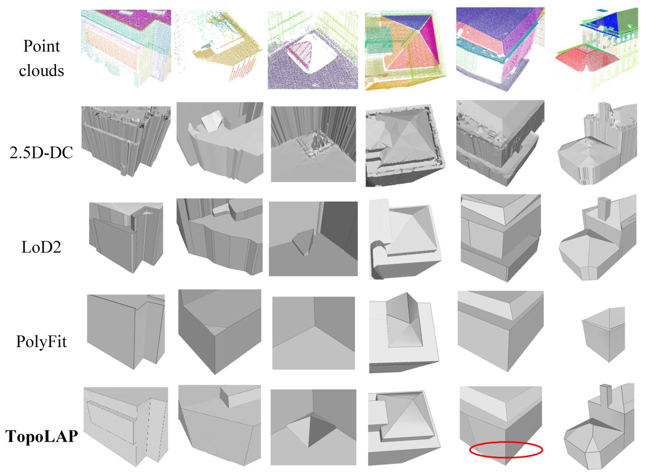
6.2. Building Reconstruction Results

The orthogonal distance from input points to their corresponding plane $P2M$ and the shortest distance from object points to input points on corresponding faces $O2P$ are used as the measures to evaluate the model fitness as concluded by [52]. $P2M$ reveals how well the input data fits to the output models and $O2P$ for the model accuracy.

To evaluate the correctness of the model, the ratio of the number of correctly reconstructed planes and the number of total planes is calculated as the correction rate, $Corr.$ The plane is identified as correct if the $O2P$ is smaller than $\mathsf{\epsilon }$. Then the correction rate of model $ℳ$ at distance $\mathsf{\epsilon }$ is formulated as:

$$Cor{r}_{\mathsf{\epsilon }}\left({\mathrm{\Omega }}_{ℳ}\right)=\frac{\#\left\{{\mathrm{\Omega }}_i\in {\mathrm{\Omega }}_{ℳ}|O2P_{mean}\left({\mathrm{\Omega }}_i\right)<\mathsf{\epsilon }\right\}}{\#\left\{{\mathrm{\Omega }}_i\in {\mathrm{\Omega }}_{ℳ}\right\}}$$

(15)

where $O2P_{mean}\left({\mathrm{\Omega }}_i\right)$ measures the mean $O2P$ distances of plane ${\mathrm{\Omega }}_i$. ${\mathrm{\Omega }}_{ℳ}$ represents the reconstructed planes of the model $ℳ$.

The proposed method, TopoLAP, is compared to three cutting-edge related works, including 2.5D dual contouring [53], a LoD2 method [21], and PolyFit. Visual results and the quantitative assessment are listed in

Table 4. Visual and quantitative comparison to the related works.

		2.5D-DC 1		LoD2		PolyFit		TopoLAP
Dublin4
$P2M_{mean}$	$P2M_{RMS}$	0.060	0.187	0.222	0.429	0.343	0.583	0.238	0.442
$O2P_{mean}$	$O2P_{RMS}$	6.56 × 10−3	0.093	4.23 × 10−3	0.069	1.86 × 10−3	0.01	1.53 × 10−3	0.024
#Planes		11,138		124		17		16
$Cor{r}_{0.05}$	$Cor{r}_{0.1}$	86.6%	91.3%	76.9%	82.3%	76.5%	76.5%	93.7%	93.7%
Ningbo
$P2M_{mean}$	$P2M_{RMS}$	0.446	0.885	0.209	0.517	0.535	0.946	0.392	0.761
$O2P_{mean}$	$O2P_{RMS}$	830 × 10−3	0.918	59 × 10−3	0.638	6.69 × 10−3	0.224	6.12 × 10−3	0.169
#Planes		1121		342		12		14
$Cor{r}_{0.05}$	$Cor{r}_{0.1}$	62.3%	67.4%	73.6%	82.1%	66.7%	66.7%	92.8%	100.0%

¹ For 2.5D dual contouring, the corresponding plane of a point is the closest facet in the model.

. Among these algorithms, the 2.5D-DC traces the boundaries of rooftops and lifts them up to form the 2.5D model of buildings, which ignores the topology information. The LoD2 algorithm reconstructs the rooftop model with more details preserved but the boundaries of each roof are deviated, which leads to lower $O2P$. In Figure 13, we give the visualization comparison for the distance evaluation. Compared to PolyFit, our method recovers the missing topology of the incomplete point clouds, especially for the bottom planes which cannot be captured by aerial systems. Quantitative results show that high accuracy, as well as a high correction rate, can be achieved in the meanwhile. More details of the comparative results are displayed in Figure 14. In general, models by the proposed method preserve less detail parts compared to the contouring or rooftop-based models since some of the façades or open walls are failed to be recovered; but the planes in our polyhedral models are of higher correctness and better fit to the original point clouds, which implies that the main frame of the building is well reconstructed and achieved a higher topological accuracy than the other methods.

The runtime of each model is displayed in Table 2, where the colorized blocks represent the steps from left to right: feature detection, structural contour extraction, plane deduction, and polyhedral model generation, respectively. The computer used for testing is a laptop running windows 10 with Intel Core CPU i7-7700HQ clocked at 2.80GHz with 24GB RAM. For the Dublin1 dataset that contains 103 planes as input, the PolyFit generates more than 176k faces, which makes the function unsolvable. Our optimized method generates only 3271 candidate faces, while the correction rate of 93.4% is achieved with acceptable runtime.

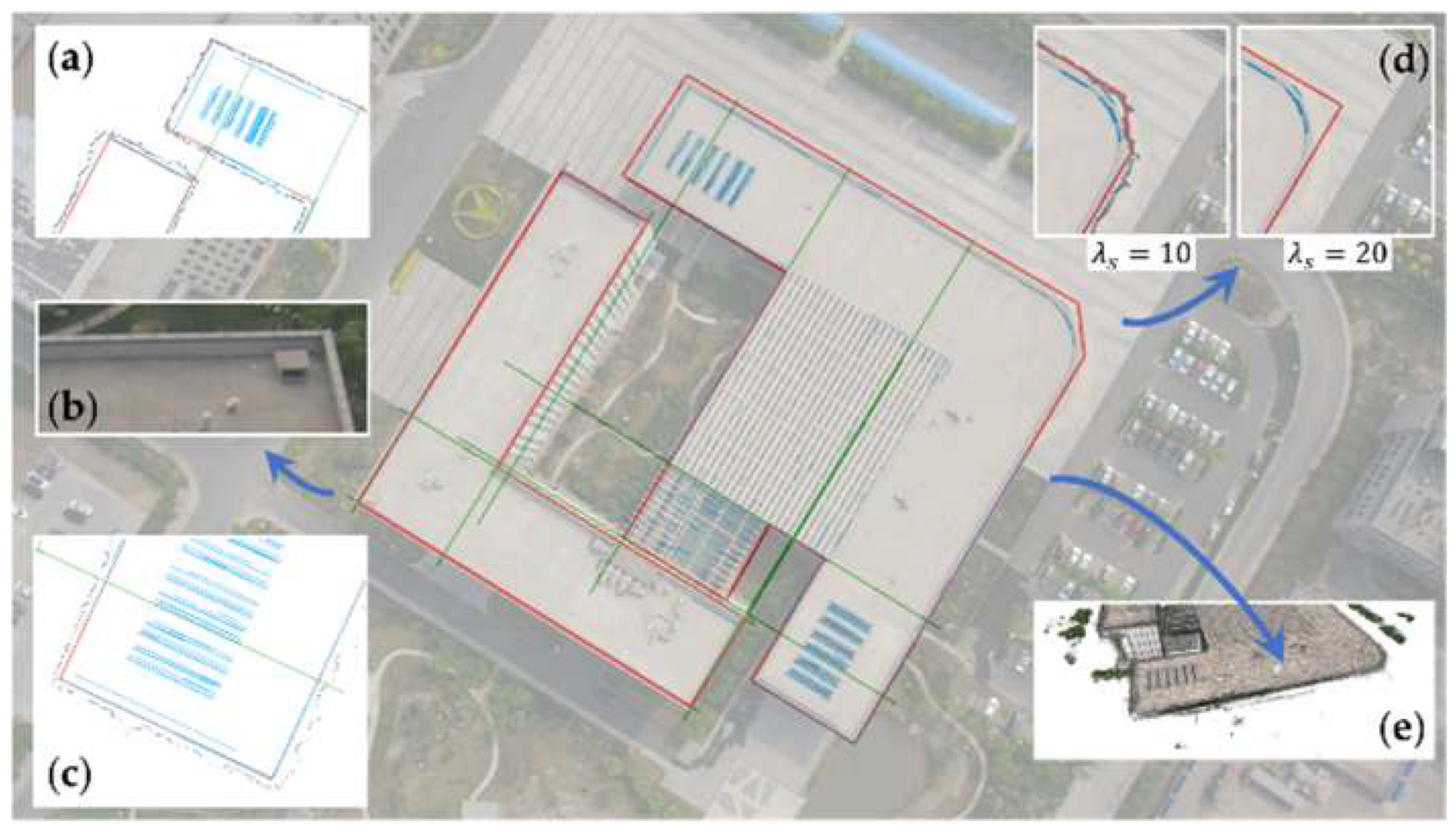
6.3. Performance Analysis of the Linear Primitives

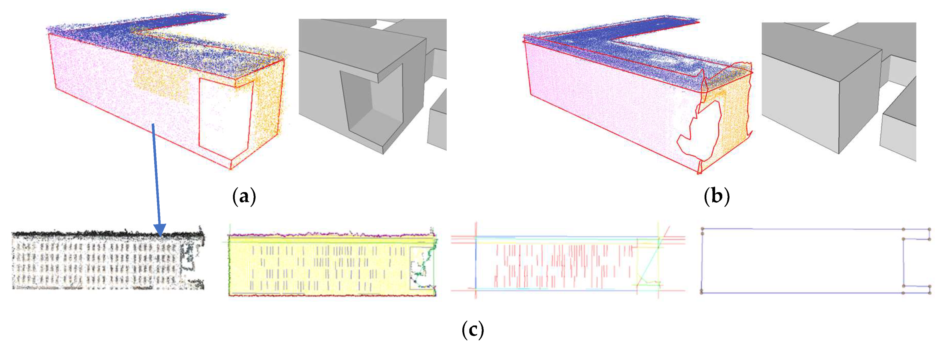
The rooftops of MVS dataset are selected to show the results of the structural contour extraction algorithm in Figure 15, and the model reconstructed based on the structural contour is compared to that using a line grow-based algorithm [18] as displayed Figure 16. The structural contours may ignore the tiny or slender parts of the boundaries such as the eave or parapet wall to preserve the mainframes of the plane, which are a substantial hint for the plane deduction. The linear primitives are merged and regularized before the candidate generation to avoid superabundant variables.

6.4. Limitations

Our method can handle incomplete point clouds and recover the partially missing planes. However, no Manhattan constraints are used so that partial covering of the façade walls are still required since the structural information is needed for the plane deduction. If only a few initial façade segments can be detected, it is hard to abstract the structural information of the plane composed by sparse points and the deducted planes are not reliable enough. In addition, to ensure the model is manifold and watertight, mainframe of the plane-based building is preserved while slender parts, open walls, subsidiary components are ignored such as eaves, parapet walls, and small chimneys, etc. (red circle in the bottom line of Figure 14 for example).

7. Conclusions

Although the acquisition devices are developed and point clouds of high density can be obtained, building reconstruction from point clouds continues to pose significant challenges. The data noise, missing data, and varying densities, etc. make it hard to reconstruct the building models with high automation, high efficiency and high precision in order to handle the multi-functional components of the buildings and the iteratively upgraded city models.

The proposed pipeline, TopoLAP, resorts to the relationships between the planar and linear primitives and generates a complete set of planes for building reconstruction. Structural contours are extracted taking full advantage of the complementary characteristics of point clouds and images. The energy minimization-based strategy stands out as an optimal trade-off solution to fit the outline to sharp lines both in the point cloud and images. The plane deduction excavates the potential planes from the impaired point clouds by analyzing the relationships of the existing planar and linear primitives. The pipeline makes it possible to efficiently reconstruct LoD3 models of both high topological and geometrical precision from partially impaired point clouds.

Although our modeling strategies optimize the plane segmentation results, the modeling result still relies on the initial segmentation, which is a common problem for primitive-based methods. Other types of geometry objects exclude planes, as well as the small planes whose point clouds are sparse and ignored by the polyhedral modeling, can be added as the subsidiary components to corresponding planes, which enables the detailed reconstruction of the complex buildings. In addition, considering the similarity of the method in indoor modeling, the proposed pipeline can also be extended to reconstruct indoor scenes. These improvements will be addressed in future works.

References

1. Biljecki, F.; Stoter, J.; Ledoux, H.; Zlatanova, S.; Çöltekin, A. Applications of 3D City Models: State of the Art Review. ISPRS Int. J. Geo-Inf. 2015, 4, 2842–2889. [Google Scholar] [CrossRef] [Green Version]
2. Haala, N.; Kada, M. An update on automatic 3D building reconstruction. ISPRS J. Photogramm. Remote Sens. 2010, 65, 570–580. [Google Scholar] [CrossRef]
3. Musialski, P.; Wimmer, M. Inverse-Procedural Methods for Urban Models. In Proceedings of the Eurographics Workshop on Urban Data Modelling and Visualisation, Girona, Spain, 5 May 2013; pp. 31–32. [Google Scholar] [CrossRef]
4. Wang, R.; Peethambaran, J.; Dong, C. LiDAR Point Clouds to 3D Urban Models: A Review. IEEE J. Sel. Top. Appl. Earth Obs. Remote Sens. 2018, 11, 606–627. [Google Scholar] [CrossRef]
5. Gröger, G.; Plümer, L. CityGML - Interoperable semantic 3D city models. ISPRS J. Photogramm. Remote Sens. 2012, 71, 12–33. [Google Scholar] [CrossRef]
6. Rottensteiner, F.; Sohn, G.; Gerke, M.; Wegner, J.D.; Breitkopf, U.; Jung, J. Results of the ISPRS benchmark on urban object detection and 3D building reconstruction. ISPRS J. Photogramm. Remote Sens. 2014, 93, 256–271. [Google Scholar] [CrossRef]
7. Salehi, A.; Mohammadzadeh, A. Building Roof Reconstruction Based on Residue Anomaly Analysis and Shape Descriptors from Lidar and Optical Data. Photogramm. Eng. Remote Sens. 2017, 83, 281–291. [Google Scholar] [CrossRef]
8. Yang, L.; Sheng, Y.; Wang, B. 3D reconstruction of building facade with fused data of terrestrial LiDAR data and optical image. Optik (Stuttg). 2016, 127, 2165–2168. [Google Scholar] [CrossRef]
9. Zhu, Q.; Li, Y.; Hu, H.; Wu, B. Robust point cloud classification based on multi-level semantic relationships for urban scenes. ISPRS J. Photogramm. Remote Sens. 2017, 129, 86–102. [Google Scholar] [CrossRef]
10. Hofer, M.; Maurer, M.; Bischof, H. Efficient 3D scene abstraction using line segments. Comput. Vis. Image Underst. 2017, 157, 167–178. [Google Scholar] [CrossRef]
11. Lin, Y.; Wang, C.; Cheng, J.; Chen, B.; Jia, F.; Chen, Z.; Li, J. Line segment extraction for large scale unorganized point clouds. ISPRS J. Photogramm. Remote Sens. 2015, 102, 172–183. [Google Scholar] [CrossRef]
12. Ni, H.; Lin, X.; Ning, X.; Zhang, J. Edge detection and feature line tracing in 3D-point clouds by analyzing geometric properties of neighborhoods. Remote Sens. 2016, 8, 710. [Google Scholar] [CrossRef]
13. Schnabel, R.; Wahl, R.; Klein, R. Efficient RANSAC for Point-Cloud Shape Detection. In Computer Graphics Forum; Wiley: Oxford, UK, 2007; Volume 26, pp. 214–226. [Google Scholar] [CrossRef]
14. Desolneux, A.; Moisan, L.; Morel, J.-M. From Gestalt Theory to Image Analysis: A Probabilistic Approach; Springer Science & Business Media: New York, NY, USA, 2007; Volume 34. [Google Scholar] [CrossRef]
15. Gómez, A.; Randall, G.; von Gioi, R.G. A contrario 3D point alignment detection algorithm. IPOL J. Image Process. Line 2017, 7, 399–417. [Google Scholar] [CrossRef]
16. Lezama, J.; Morel, J.M.; Randall, G.; Grompone Von Gioi, R. A contrario 2D point alignment detection. IEEE Trans. Pattern Anal. Mach. Intell. 2015, 37, 499–512. [Google Scholar] [CrossRef]
17. Hackel, T.; Wegner, J.D.; Schindler, K. Joint classification and contour extraction of large 3D point clouds. ISPRS J. Photogramm. Remote Sens. 2017, 130, 231–245. [Google Scholar] [CrossRef]
18. Cao, R.; Zhang, Y.; Liu, X.; Zhao, Z. 3D building roof reconstruction from airborne LiDAR point clouds: A framework based on a spatial database. Int. J. Geogr. Inf. Sci. 2017, 31, 1359–1380. [Google Scholar] [CrossRef]
19. Cao, R.; Zhang, Y.; Liu, X.; Zhao, Z. Roof plane extraction from airborne lidar point clouds. Int. J. Remote Sens. 2017, 38, 3684–3703. [Google Scholar] [CrossRef]
20. Wang, J.; Fang, T.; Su, Q.; Zhu, S.; Liu, J.; Cai, S.; Tai, C.L.; Quan, L. Image-Based Building Regularization Using Structural Linear Features. IEEE Trans. Vis. Comput. Graph. 2016, 22, 1760–1772. [Google Scholar] [CrossRef]
21. Xiong, B.; Oude Elberink, S.; Vosselman, G. Building modeling from noisy photogrammetric point clouds. ISPRS Ann. Photogramm. Remote Sens. Spat. Inf. Sci. 2014, II-3, 197–204. [Google Scholar] [CrossRef] [Green Version]
22. Xu, Y.; Wu, L.; Xie, Z.; Chen, Z. Building Extraction in Very High Resolution Remote Sensing Imagery Using Deep Learning. Remote Sens. 2018, 10, 144. [Google Scholar] [CrossRef]
23. Isack, H.; Boykov, Y. Energy-based geometric multi-model fitting. Int. J. Comput. Vis. 2012, 97, 123–147. [Google Scholar] [CrossRef]
24. Li, Y.; Wu, X.; Chrysathou, Y.; Sharf, A.; Cohen-Or, D.; Mitra, N.J. GlobFit: Consistently Fitting Primitives by Discovering Global Relations. ACM Trans. Graph. 2011, 30, 1. [Google Scholar] [CrossRef]
25. Monszpart, A.; Mellado, N.; Brostow, G.J.; Mitra, N.J. RAPter: Rebuilding Man-made Scenes with Regular Arrangements of Planes. ACM Trans. Graph. 2015, 34, 103:1–103:12. [Google Scholar] [CrossRef]
26. Boulch, A.; de La Gorce, M.; Marlet, R. Piecewise-planar 3D reconstruction with edge and corner regularization. Eurographics Symp. Geom. Process. 2014, 33, 55–64. [Google Scholar] [CrossRef]
27. Oesau, S.; Lafarge, F.; Alliez, P. Planar shape detection and regularization in tandem. In Computer Graphics Forum; Wiley: Zürich, Switzerland, 2016; Volume 35, pp. 203–215. [Google Scholar] [CrossRef]
28. Holzmann, T.; Maurer, M.; Fraundorfer, F.; Bischof, H. Semantically aware urban 3d reconstruction with plane-based regularization. In Proceedings of the European Conference on Computer Vision, Munich, Germany, 8–14 September 2018; pp. 487–503. [Google Scholar]
29. Coughlan, J.M.; Yuille, A.L. Manhattan World: compass direction from a single image by Bayesian inference. In Proceedings of the Seventh IEEE International Conference on Computer Vision, Kerkyra, Greece, 20–27 September 1999; Volume 2, pp. 941–947. [Google Scholar] [CrossRef]
30. Nan, L.; Sharf, A.; Zhang, H.; Cohen-Or, D.; Chen, B. SmartBoxes for interactive urban reconstruction. ACM Trans. Graph. 2010, 29, 1. [Google Scholar] [CrossRef]
31. Oesau, S.; Lafarge, F.; Alliez, P. Indoor scene reconstruction using feature sensitive primitive extraction and graph-cut. ISPRS J. Photogramm. Remote Sens. 2014, 90, 68–82. [Google Scholar] [CrossRef] [Green Version]
32. Elberink, S.O.; Vosselman, G. Building reconstruction by target based graph matching on incomplete laser data: Analysis and limitations. Sensors 2009, 9, 6101–6118. [Google Scholar] [CrossRef]
33. Perera, G.S.N.; Maas, H.G. Cycle graph analysis for 3D roof structure modelling: Concepts and performance. ISPRS J. Photogramm. Remote Sens. 2014, 93, 213–226. [Google Scholar] [CrossRef]
34. Xu, B.; Jiang, W.; Li, L. HRTT: A hierarchical roof topology structure for robust building roof reconstruction from point clouds. Remote Sens. 2017, 9, 354. [Google Scholar] [CrossRef]
35. Nan, L.; Wonka, P. PolyFit: Polygonal Surface Reconstruction from Point Clouds. In Proceedings of the 2017 IEEE International Conference on Computer Vision, Venice, Italy, 22–29 October 2017; pp. 2353–2361. [Google Scholar]
36. Zolanvari, S.M.I.; Laefer, D.F.; Natanzi, A.S. Three-dimensional building façade segmentation and opening area detection from point clouds. ISPRS J. Photogramm. Remote Sens. 2018, 143, 134–149. [Google Scholar] [CrossRef]
37. Xiong, B.; Oude Elberink, S.; Vosselman, G. A graph edit dictionary for correcting errors in roof topology graphs reconstructed from point clouds. ISPRS J. Photogramm. Remote Sens. 2014, 93, 227–242. [Google Scholar] [CrossRef]
38. Xiong, B.; Jancosek, M.; Oude Elberink, S.; Vosselman, G. Flexible building primitives for 3D building modeling. ISPRS J. Photogramm. Remote Sens. 2015, 101, 275–290. [Google Scholar] [CrossRef]
39. Li, M.; Wonka, P.; Nan, L. Manhattan-world urban reconstruction from point clouds. In European Conference on Computer Vision; Springer: Amsterdam, The Netherlands, 2016; pp. 54–69. [Google Scholar]
40. Gao, X.; Shen, S.; Zhou, Y.; Cui, H.; Zhu, L.; Hu, Z. Ancient Chinese architecture 3D preservation by merging ground and aerial point clouds. ISPRS J. Photogramm. Remote Sens. 2018. [Google Scholar] [CrossRef]
41. Gao, X.; Shen, S.; Hu, Z.; Wang, Z. Ground and aerial meta-data integration for localization and reconstruction: A review. Pattern Recognit. Lett. 2018, 1–13. [Google Scholar] [CrossRef]
42. Sakurada, K.; Tetsuka, D.; Okatani, T. Temporal city modeling using street level imagery. Comput. Vis. Image Underst. 2017, 157, 55–71. [Google Scholar] [CrossRef]
43. Zhang, S.; Tao, P.; Wang, L.; Hou, Y.; Hu, Z. Improving Details of Building Façades in Open LiDAR Data Using Ground Images. Remote Sens. 2019, 11, 420. [Google Scholar] [CrossRef]
44. Arikan, M.; Schwärzler, M.; Flöry, S.; Wimmer, M.; Maierhofer, S. O-snap: Optimization-based snapping for modeling architecture. ACM Trans. Graph. 2013, 32, 1–15. [Google Scholar] [CrossRef]
45. Ochmann, S.; Vock, R.; Klein, R. Automatic reconstruction of fully volumetric 3D building models from oriented point clouds. ISPRS J. Photogramm. Remote Sens. 2019, 151, 251–262. [Google Scholar] [CrossRef] [Green Version]
46. Boykov, Y.; Veksler, O.; Zabih, R. Fast approximate energy minimization via graph cuts. IEEE Trans. Pattern Anal. Mach. Intell. 2001, 23, 1. [Google Scholar] [CrossRef]
47. Grompone Von Gioi, R.; Jakubowicz, J.; Morel, J.M.; Randall, G. LSD: A fast line segment detector with a false detection control. IEEE Trans. Pattern Anal. Mach. Intell. 2010, 32, 722–732. [Google Scholar] [CrossRef]
48. Wang, Z.; Liu, H.; Wu, F. MSLD: A robust descriptor for line matching. In Proceedings of the 2009 11th IEEE International Conference on Computer-Aided Design and Computer Graphics, Huangshan, China, 19–21 August 2009; Volume 42, pp. 128–133. [Google Scholar] [CrossRef]
49. Lyu, C.; Jiang, J. Remote sensing image registration with line segments and their intersections. Remote Sens. 2017, 9, 439. [Google Scholar] [CrossRef]
50. ALSDublin ALSDublin15. Available online: https://serv.cusp.nyu.edu/projects/ALSDublin15/ALSDublin15.html (accessed on 4 June 2019).
51. Fuhrmann, S.; Langguth, F.; Goesele, M. MVE-A Multi-View Reconstruction Environment. EUROGRAPHICS Work. Graph. Cult. Herit. 2014, 11–18. [Google Scholar] [CrossRef]
52. Oude Elberink, S.; Vosselman, G. Quality analysis on 3D building models reconstructed from airborne laser scanning data. ISPRS J. Photogramm. Remote Sens. 2011, 66, 157–165. [Google Scholar] [CrossRef]
53. Zhou, Q.-Y.; Neumann, U. 2.5 d dual contouring: A robust approach to creating building models from aerial lidar point clouds. In European Conference on Computer Vision; Springer: Berlin/Heidelberg, Germany, 2010; pp. 115–128. [Google Scholar]
Figure 1. Examples of complex building structures and incomplete planar primitives. Colors are randomly set for different planes and the black dots denote unsegmented points. Points of the façade inside the red oval are missing. (a) Planar segments are lost due to the partial sparsity. (b) Without the constraint of the façade, the outward boundaries are inaccurate by rooftop modeling.
Remotesensing 11 01372 g001
Figure 2. The pipeline of the LoD3 building reconstruction from point clouds.
Remotesensing 11 01372 g002
Figure 3. Visualization of the characteristics of three different feature lines and the optimized structural contours extracted from these feature lines. (a) Image lines: high geometric precision, non-topological, incomplete. (b) Intersection lines: topological support, incomplete, low correction rate. (c) Boundary lines: complete, poor topological support, low geometric precision. (d) Structural contours: optimized results.
Remotesensing 11 01372 g003
Figure 4. Boundary points estimation in k nearest neighbors (k = 16). (a) The red point is identified as a boundary point. (b) Points are down-sampled to 1000 points (green) with 164 boundary points (red) detected. (c) The original 77,835 points (green) with 1448 boundary points (red) detected.
Remotesensing 11 01372 g004
Figure 5. Illustration of the calculation of the point distribution.
Remotesensing 11 01372 g005
Figure 6. Banded line-support region for line l . B G M i indicates the weighted mean vector of , the gradient projected on the direction of the normal vector.
Remotesensing 11 01372 g006
Figure 7. An illustration of the data term and the selection strategy. (a) Candidates rendered by the value of the distribution. (b) Candidates rendered by the value of sharpness. (c) Candidates rendered by the value of the data term. Candidates whose endpoint is 1-link or too close to other candidates are excluded from data term calculation. (d) Optimization result.
Remotesensing 11 01372 g007
Figure 8. Example of the Line-and-Line Unit validation. (a) Red lines represent the convex hull; black lines are identified as Border Lines while the rest blue ones the Inner Edges. (b) Plane B 1 B C C 1 is validated by the LaL Unit B 1 B - B C - C C 1 .
Remotesensing 11 01372 g008
Figure 9. Validation criterions for Line-and-Line Unit.
Remotesensing 11 01372 g009
Figure 10. The workflow of the plane deduction.
Remotesensing 11 01372 g010
Figure 11. The pipeline to construct planes by plane deduction. (a) The LaP group segmented by plane detection from lines. (b) Validated LaL unit on the LaP group. (c) The structural contour of the validated LaP. (d) Another two new planes validated by the next iteration.
Remotesensing 11 01372 g011
Figure 12. Invalid face elimination in a single plane. (a) The original candidate faces of a planar primitive generated by intersection. (b) The valid candidate faces after elimination. The black frame delineates the merged boundary of the original plane and the polygon colors are rendered by the confidence of each candidate face in PolyFit from red (high) to blue (low). (c) The remaining plane candidates, from which the planes of the final polyhedral models are selected (refer to Dublin2 in Table 1 for the original points and the final model).
Remotesensing 11 01372 g012
Figure 13. Visualization of the distance evaluation for Dublin1 compared to the LoD2 model.
Remotesensing 11 01372 g013
Figure 14. Comparative results of selected details.
Remotesensing 11 01372 g014
Figure 15. Optimized rooftop contours superimposed on the image. (a) The original boundary line is kept, not fitting to the image line which is the inner boundary. (b) The boundary of the façade is extruded upwards from the rooftop; thus, the intersection line is not the accurate upper outline of the adjacent façade. (c) The boundary line is snapped to the closest image line which represents the outer boundary. (d) The influence of the smooth-term coefficient. (e) The intersection information is lost in the absence of the adjacent façade.
Remotesensing 11 01372 g015
Figure 16. Model correctness comparison based on different linear primitives. The top row displays the corresponding models reconstructed from the structural contours (a) and the line grow-based contours (b), respectively. Planes inside the corner can be deduced based on the structural contours. And (c) displays the optimization progress of the front façade. From left to right: original points of the plane, three types of feature lines, the lines rendered by data-term, and the optimized structural contours.
Remotesensing 11 01372 g016