Deep Transfer Learning for Few-Shot SAR Image Classification


1
HRL Laboratories, Malibu, CA 90265-4797, USA
2
Department of Computer and Information Science, University of Pennsylvania, Philadelphia, PA 19104, USA
*
Author to whom correspondence should be addressed.
Remote Sens. 2019, 11(11), 1374; https://0-doi-org.brum.beds.ac.uk/10.3390/rs11111374
Submission received: 30 April 2019
/
Revised: 30 May 2019
/
Accepted: 5 June 2019
/
Published: 8 June 2019
(This article belongs to the Special Issue Deep Transfer Learning for Remote Sensing)
Abstract
:The reemergence of Deep Neural Networks (DNNs) has lead to high-performance supervised learning algorithms for the Electro-Optical (EO) domain classification and detection problems. This success is because generating huge labeled datasets has become possible using modern crowdsourcing labeling platforms such as Amazon’s Mechanical Turk that recruit ordinary people to label data. Unlike the EO domain, labeling the Synthetic Aperture Radar (SAR) domain data can be much more challenging, and for various reasons, using crowdsourcing platforms is not feasible for labeling the SAR domain data. As a result, training deep networks using supervised learning is more challenging in the SAR domain. In the paper, we present a new framework to train a deep neural network for classifying Synthetic Aperture Radar (SAR) images by eliminating the need for a huge labeled dataset. Our idea is based on transferring knowledge from a related EO domain problem, where labeled data are easy to obtain. We transfer knowledge from the EO domain through learning a shared invariant cross-domain embedding space that is also discriminative for classification. To this end, we train two deep encoders that are coupled through their last year to map data points from the EO and the SAR domains to the shared embedding space such that the distance between the distributions of the two domains is minimized in the latent embedding space. We use the Sliced Wasserstein Distance (SWD) to measure and minimize the distance between these two distributions and use a limited number of SAR label data points to match the distributions class-conditionally. As a result of this training procedure, a classifier trained from the embedding space to the label space using mostly the EO data would generalize well on the SAR domain. We provide a theoretical analysis to demonstrate why our approach is effective and validate our algorithm on the problem of ship classification in the SAR domain by comparing against several other competing learning approaches.
1. Introduction
Historically and prior to the emergence of machine learning, most imaging devices were designed first to generate outputs that were interpretable by humans, mostly natural images. As a result, the dominant visual data that are collected even currently are the Electro-Optical (EO) domain data. Digital EO images are generated by a planner grid of sensors that detect and record the magnitude and the color of reflected visible light from the surface of an object in the from of a planner array of pixels. Naturally, most machine learning algorithms that are developed for automation also process EO domain data as their input. Recently, the area of EO-based machine learning and computer vision has been successful in developing classification and detection algorithms with human-level performance for many applications. In particular, reemergence of neural networks in the form deep Convolutional Neural Networks (CNNs) has been crucial for this success. The major reason for the outperformance of CNNs over many prior classic learning methods is that the time-consuming and unclear procedure of feature engineering in classic machine learning and computer vision can be bypassed when CNNs are trained. CNNs are able to extract abstract and high-quality discriminative features for a given task automatically in a blind end-to-end supervised training scheme, where CNNs are trained using a huge labeled dataset of images. Since the learned features are task-dependent, this often leads to better performance compared to engineered features that are usually defined for a broad range of tasks, e.g., wavelet, DFT, SIFT, etc. Partial early results of this work will be presented at the 2019 CVPR workshop on Perception Beyond the Visible Spectrum [1].
Despite wide range of applicability of EO imaging, it is also naturally constrained by the limitations of the human visual sensory system. In particular, in applications such as continuous environmental monitoring and large-scale surveillance [2] and Earth remote sensing [3], continuous imaging for extended time periods and independent of the weather conditions is necessary. EO imaging is not suitable for such applications because imaging during night and cloudy weather is not feasible. In these applications, using other imaging techniques that are designed for imaging beyond the visible spectrum is inevitable. Synthetic Aperture Radar (SAR) imaging is a major technique in this area that is highly effective for remote sensing applications. SAR imaging benefits from radar signals that can propagate in occluded weather and at night. Radar signals are emitted sequentially from a moving antenna, and the reflected signals are collected for subsequent signal processing to generate high-resolution images irrespective of the weather conditions and occlusions. While both the EO and the SAR domain images describe the same physical world and often SAR data are represented in a planner array form similar to an EO image, processing EO and SAR data and developing suitable learning algorithms for these domains can be quite different. In particular, replicating the success of CNNs in supervised learning problems of the SAR domain is more challenging. This is because training CNNs is conditioned on the availability of huge labeled datasets to supervise blind end-to-end learning. Until quite recently, generating such datasets was challenging and expensive. Currently, labeled datasets for the EO domain tasks are generated using crowdsourcing labeling platforms such as Amazon’s Mechanical Turk, e.g., ImageNet [4]. In a crowdsourcing platform, a pool of participants with common basic knowledge for labeling EO data points, i.e., natural images, is recruited. These participants need minimal training and in many cases are not even compensated for their time and effort. Unlabeled images are presented to each participant independently, and each participant selects a label for each given image. Upon collecting labels from several people from the pool of participants, the collected labels are aggregated according to the skills and reliability of each participant to increase labeling accuracy [5]. Despite being very effective at generating high quality labeled datasets for EO domains, for various reasons, crowdsourcing platforms are not suitable for SAR domains:
- Preparing devices for collecting SAR data, solely for generating training datasets, is much more expensive compared to EO datasets [6]. In many cases, EO datasets can even be generated from the Internet using existing images that are taken by commercial cameras. In contrast, SAR imaging devices are not commercial and usually are expensive to operate, e.g., satellites.
- SAR images are often classified data because for many applications, the goal is surveillance and target detection. This issue makes access to SAR data heavily regulated and limited to certified people. Even for research purposes, only a few datasets are publicly available. This limits the number of participants who can be hired to help with processing and labeling.
- Despite similarities, SAR images are not easy to interpret by an average person. For this reason, labeling SAR images requires trained experts who know how to interpret SAR data. This is in contrast with tasks within the EO domain images, where ordinary people can label images with minimal training and guidance [7]. This challenge makes labeling SAR data more expensive, as only professional trained people can perform labeling of SAR data.
- Continuous collection of SAR data is common in SAR applications. As a result, the distribution of data is likely to be non-stationery. As a result, even a high-quality labeled dataset is generated, and the data would become unrepresentative of the current distribution over extended time intervals. This would obligate persistent data labeling to updated a trained model [8].
As a result of the above challenges, generating labeled detests for the SAR domain data is in general difficult. In particular, given the size of most existing SAR datasets, training a CNN leads to overfit models, as the number of data points is considerably less than the required sample complexity of training a deep network [9,10]. When the model is overfit, naturally, it will not generalize well on test sets. In other words, we face situations in which the amount of accessible labeled SAR data is not sufficient for training deep neural networks that extract useful features. In the machine learning literature, the challenges of learning in this scenario have been investigated within transfer learning [11]. The general idea that we focus on is to transfer knowledge from a secondary domain to reduce the amount labeled data that are necessary to train a model. Building upon prior works in the area of transfer learning, several recent works have used the idea of knowledge transfer to address the challenges of SAR domains [6,8,10,12,13,14]. The common idea in these works is to transfer knowledge from a secondary related problem, where labeled data are easy and inexpensive to obtain. For example, the second domain can be a related task in the EO domain or a task generated by synthetic data. Following this line of work, our goal in this paper is to tackle the challenges of learning in SAR domains when the labeled data are scarce. This particular setting of transfer learning is also called domain adaptation in the machine learning literature. In this setting, the domain with labeled data scarcity is called the source domain, and the domain with sufficient labeled data is called the target domain. We develop a method that benefits from cross-domain knowledge transfer from a related task in EO domains as the source domain to address a task in SAR domains as the target domain. More specifically, we consider a classification task with the same classes in two domains, i.e., SAR and EO. This is a typical situation for many applications, as it is common to use both SAR and EO imaging. We consider a domain adaptation setting, where we have sufficient labeled data points in the source domain, i.e., EO. We also have access to abundant data points in the target domain, i.e., EO, but only a few labeled data points are labeled. This setting is called semi-supervised domain adaptation in the machine learning literature [15].
Several approaches have been developed to address the problem of domain adaptation. A common technique for cross-domain knowledge transfer is to encode the data points of the two related domains in a domain-invariant embedding space such that similarities between the tasks can be identified and captured in the shared space. As a result, knowledge can be transferred across the domains in the embedding space through correspondences that are captured between the domains in the shared space. The key challenge is how to find such an embedding space. In this paper, we model the shared embedding space as the output space of deep encoders. We couple two deep encoders to map the data points from the EO and the SAR domains into a shared embedding space as their outputs such that both domains would have similar distributions in this space. If both domains have similar class-conditional probability distributions in the embedding space, then if we train a classifier network using only the source domain labeled data points from the shared embedding to the label space, it will also generalize well on the target domain test data points [16]. This goal can be achieved by training the deep encoders as two deterministic functions using training data such that the empirical distribution discrepancy between the two domains is minimized in the shared output of the deep encoders with respect to some probability distribution metric [17,18].
Our contribution is to propose a novel semi-supervised domain adaptation algorithm to transfer knowledge from the EO domain to the SAR domain using the above explained procedure. We train the encoder networks by using the Sliced Wasserstein Distance (SWD) [19] to measure and then minimize the discrepancy between the source and the target domain distributions. There are two majors reasons for using SWD. First, SWD is an effective metric for the space of probability distributions that can be computed efficiently. Second, SWD is non-zero even for two probability distributions with non-overlapping supports. As a result, it has non-vanishing gradients, and first-order gradient-based optimization algorithms can be used to solve optimization problems involving SWD terms [16,20]. This is important, as most optimization problems for training deep neural networks are solved using gradient-based methods, e.g., Stochastic Gradient Descent (SGD). The above procedure might not succeed because, while the distance between distributions may be minimized, they may not be aligned class-conditionally. We use the few accessible labeled data points in the SAR domain to align both distribution’s class-conditionally to tackle the class matching challenge [21]. We demonstrate theoretically why our approach is able to train a classifier with generalizability on the target SAR domain. We also provide experimental results to validate our approach in the area of maritime domain awareness, where the goal is to understand activities that could impact the safety and the environment. Our results demonstrate that our approach is effective and leads to state-of-the-art performance.
2. Related Work
Recently, several prior works have addressed classification in the SAR domain in a label-scarce regime. Huang et al. [8] used an unsupervised learning approach to generate discriminative features. Given that generating unlabeled SAR data is easier, their idea was to train a deep autoencoder using a large pool of unlabeled SAR data. Upon training the autoencoder, features extracted in the middle-layer of the autoencoder captured difference across different classes and could be used for classification. For example, the trained encoder sub-network of the autoencoder can be concatenated with a classifier network, and both would be fine-tuned using the labeled portion of data to map the data points to the label space. In other words, the deep encoder is used as a task-dependent feature extractor. Hansen et al. [6] proposed to transfer knowledge using synthetic SAR images, which are easy to generate and are similar to real images. Their idea was to to generate a simulated dataset for a given SAR problem based on simulated object radar reflectivity. Upon generating the synthetic labeled dataset, it could be used to pretrain a CNN network prior to presenting the real data. The pretrained CNN then could be used as an initialization for the real SAR domain problem. Due to the pretraining stage and similarities between the synthetic and the read data, the model can be thought of as a better initial point and hence fine-tuned using fewer real labeled data points. Zhang et al. [12] proposed to transfer knowledge from a secondary source SAR task, where labeled data are available. Similarly, a CNN network can be pretrained on the task with labeled data and then fine-tuned on the target task. Lang et al. [14] used the Automatic Identification System (AIS) as the secondary domain for knowledge transfer. AIS is a tracking system for monitoring movement of ships that can provide labeling information. Shang et al. [10] amended a CNN with an information recorder. The recorder was used to store spatial features of labeled samples, and the recorded features were used to predict the labels of unlabeled data points based on spatial similarity to increase the number of labeled samples. Finally, Weng et al. [13] used an approach more similar to our framework. Their proposal was to transfer knowledge from the EO domain using VGGNet as a feature extractor in the learning pipeline, which itself has been pretrained on a large EO dataset. Despite being effective, the common idea of these past works is mostly using a deep network that is pretrained using a secondary source of knowledge, which is then fine-tuned using a few labeled data points on the target SAR task. Hence, knowledge transfer occurs as a result of selecting a better initial point for the optimization problem using the secondary source. We follow a different approach by recasting the problem as a Domain Adaptation (DA) problem [18], where the goal is to adapt a model trained on the source domain to generalize well in the target domain. Our contribution is to demonstrate how to transfer knowledge from the EO imaging domain in order to train a deep network for the SAR domain. The idea is to use a related EO domain problem with abundant labeled data when training a deep network on a related EO problem with abundant labeled data and simultaneously adapting the model considering that only a few labeled SAR data points are accessible. In our training scheme, we enforce the distributions of both domains to become similar within a middle layer of the deep network.
Domain adaptation has been investigated in the computer vision literature for a broad range of applications for EO domain problems. The goal in domain adaptation is to train a model on a source data distribution with sufficient labeled data such that it generalizes well on a different, but related target data distribution, where labeling data is challenging. Despite being different, the common idea of DA approaches is to preprocess data from both domains or at least the target domain such that the distributions of both domains become similar after preprocessing. A classifier that is trained using the source data can also be used on the target domain due to post-processing similar distributions. In this paper, we consider that two deep convolutional neural networks preprocess data to enforce both the EO and SAR domains’ data to have similar probability distributions. To this end, we couple two deep encoder sub-networks with a shared output space to model the embedding space. This space can be considered as an intermediate embedding space between the input space from each domain and the label space of a classifier network that is shared between the two domains. These deep encoders are trained such that the discrepancy between the source and the target domain distributions is minimized in the shared embedding space, while overall classification is supervised mostly via the EO domain labeled data. This procedure can be done via adversarial learning [22], where the distributions are matched indirectly. We can also formulate an optimization problem with a probability matching objective to match the distributions directly [23]. We use the latter approach in this paper.
In order to minimize the distance between two probability distributions, we need to select a measure of distance between two empirical distributions and then minimize it using the training data from both domains. Early works in domain adaptation used the Maximum Mean Discrepancy (MMD) metric for this purpose [18]. MMD measures the distance between two distributions as the Euclidean distance between their means. However, MMD might not be an accurate measure when the distributions are multi-modal. While other well-studied discrepancy measures such as KL-divergence and Jensen–Shannon divergence have been used for a broad range of domain adaptation problems [24], these measures have vanishing gradients when the distributions have non-overlapping support. This situation can occur in initial iterations of training when the distributions are still distant. This problem makes KL-divergence and Jensen–Shannon divergence inappropriate for deep learning, as deep networks are trained using gradient-based first-order optimization techniques, which require gradient information [25]. For this reason, in recent works, the Wasserstein Distance (WD) metric [17] has gained interest as an objective function to match distributions in the deep learning community. WD has a non-vanishing gradient, but it does not have a closed-form definition and is defined as a Linear Programming (LP) problem. Solving the LP problem can be computationally expensive for high-dimensional distributions. For this reason, there is also interest in computing or approximating WD to reduce the computational burden. In this paper, we use the Sliced Wasserstein Distance (SWD) to circumvent this challenge. SWD approximates WD as the sum of multiple Wasserstein distances of one-dimensional distributions that possess a closed-form solution and can be computed efficiently [19,25,26,27].
3. Problem Formulation and Rationale
Let denote the domain space of SAR data. Consider a multiclass SAR classification problem with k classes in this domain, where i.i.d. data pairs are drawn from the joint probability distribution, i.e., , which has the marginal distribution over . Here, a label identifies the class membership of the vectorized SAR image to one of the k classes. We have access to unlabeled images in this target domain. Additionally, we have have access to O labeled images , where and contains the corresponding one-hot labels. The goal is to train a parameterized classifier , i.e., a deep neural network with weight parameters , on this domain. Given that we have access to only a few labeled data points and considering the model complexity of deep neural networks, training the deep network such that it generalizes well using solely the SAR labeled data is not feasible, as training would lead to overfitting on the few labeled data points such that the trained network would generalize poorly on test data points.
To tackle the problem of label scarcity, we considered a domain adaptation scenario. We assumed that a related source EO domain problem exists, were we have access to sufficient labeled data points such that training a generalizable model is feasible. Let denote the EO domain and denote the dataset in the EO domain, with and (), which is drawn from the marginal distribution . Note that since we consider the same cross-domain classes, we are considering the same classification problem in two domains. This cross-domain similarity is necessary for making knowledge transfer feasible. In other words, we have a classification problem with bi-modal data, but there is no point-wise correspondence across the data modals; and most data points in one of them are unlabeled. We assumed the source samples were drawn i.i.d. from the source joint probability distribution , which has the marginal distribution . Note that despite similarities between the domains, the marginal distributions of the domains are different. Given that extensive research and investigation has been done in EO domains, we hypothesized that finding such a labeled dataset was likely feasible or labeling such EO data was easier than labeling more SAR data points. Our goal was to use the similarity between the EO and the SAR domains and benefit from the unlabeled SAR data to train a model for classifying SAR images using the knowledge that can be learned from the EO domain.
Since we had access to sufficient labeled source data, training a parametric classifier for the source domain was a straightforward supervised learning problem. Usually, we solved for an optimal parameter to select the best model from the family of parametric functions . We can solve for an optimal parameter by minimizing the average empirical risk on the training labeled data points, i.e., Empirical Risk Minimization (ERM):
where is a proper loss function (e.g., cross-entropy loss). Given enough training data points, the empirical risk is a suitable surrogate for the real risk function:
which is the objective function for the Bayes optimal inference. This means that the trained classifier would generalize well on data points if they are drawn from . A naive approach to transfer knowledge from the EO domain to the SAR domain is to use of the classifier that is trained on the EO domain directly in the target domain. However, since distribution discrepancy exists between the two domains, i.e., , the trained classifier on the source domain might not generalize well on the target domain. Therefore, there is a need to adapt the training procedure for . The simplest approach that has been used in most prior works is to fine-tune the EO classifier using the few labeled target data points to employ the model in the target domain. This approach would add the constraint of , as the same input space is required to use the same network across the domains. Usually, it is easy to use image interpolation to enforce this condition, but information may be lost after interpolation. We wanted to use a more principled approach and remove the condition of . More importantly, when fine-tuning is used, unlabeled data are not used. We wanted to take advantage and benefit from the unlabeled SAR data points that are accessible and provide additional information about the SAR domain marginal distribution.
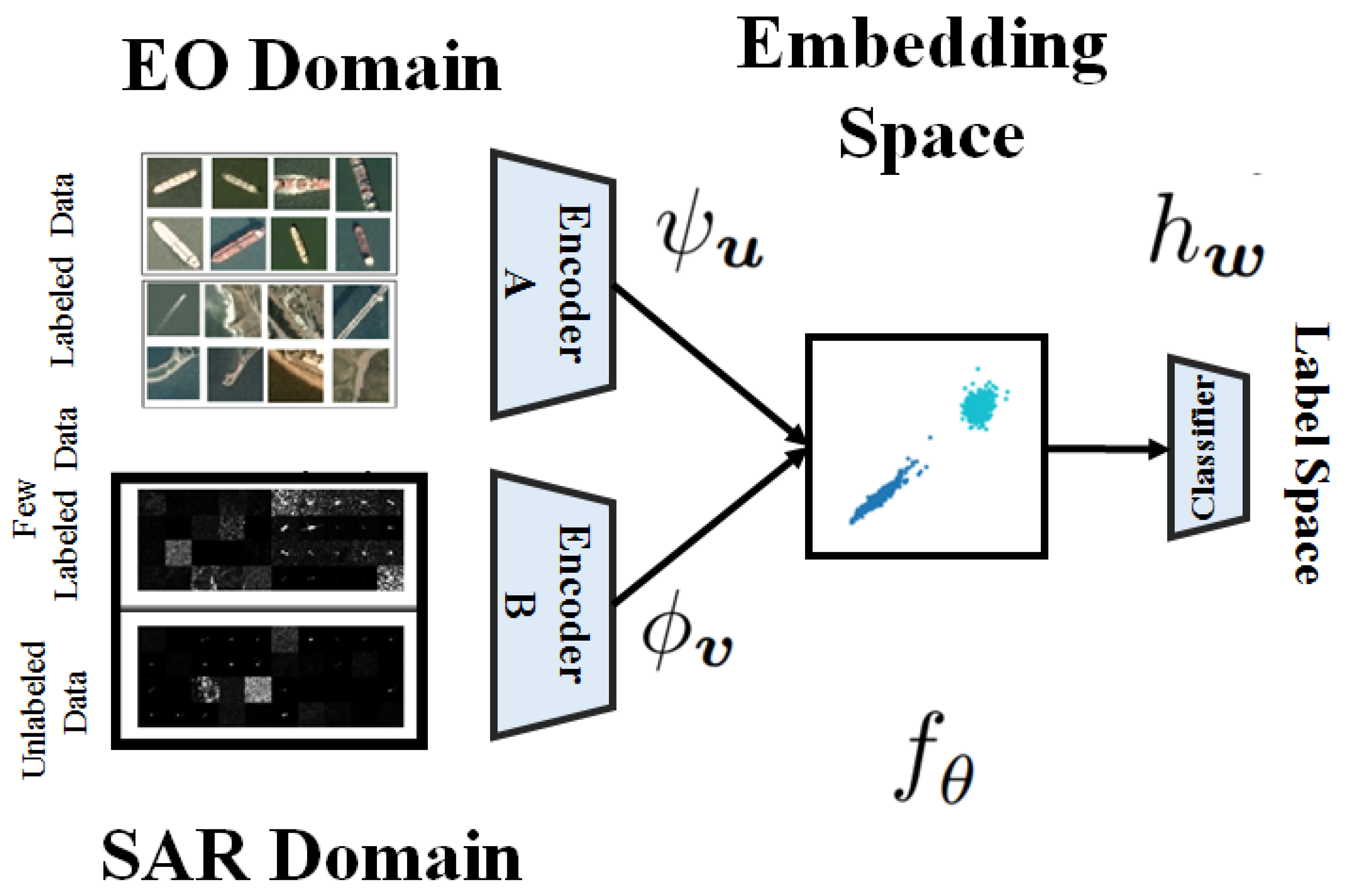
Figure 1 presents a block diagram visualization of our framework. In the figure, we have visualized images from two related real-world SAR and EO datasets that we have used in the experimental section of the paper. The task is to classify ship images. Notice that SAR images are confusing for the untrained human eye, while EO ship/no-ship images can be distinguished by minimal inspection. This suggests that, as we discussed before, SAR labeling is more challenging and requires expertise. In our approach, we considered the EO deep network to be formed by a feature extractor , i.e., convolutional layers of the network, which was followed by a classifier sub-network , i.e., fully-connected layers of the network, that inputs the extracted feature and maps them to the label space. Here, and denote the corresponding learnable parameters for these sub-networks, i.e., . This decomposition is synthetic, but helps to understand our approach. In other words, the feature extractor sub-network maps the data points into a discriminative embedding space , where classification can be done easily by the classifier sub-network . The success of deep learning stems from optimal feature extraction, which converts the data distribution into a multimodal distribution, which makes class separation feasible. Following the above, we can consider a second encoder network , which maps the SAR data points to the same target embedding space at its output. The idea that we want to explore is based on training and such that the discrepancy between the source distribution and target distribution is minimized in the shared embedding space, modeled as the shared output space of these two encoders. As a result of matching the two distributions, the embedding space becomes invariant with respect to the domain. In other words, data points from the two domains become indistinguishable in the embedding space, e.g., data points belonging to the same class are mapped into the same geometric cluster in the shared embedding space, as depicted in Figure 1. Consequently, even if we trained the classifier sub-network using solely the source labeled data points, it would still generalize well when target data points are used for testing. The key question is how to train the encoder sub-networks such that the embedding space becomes invariant. We need to adapt the standard supervised learning in Equation (1) by adding additional terms that enforce cross-domain distribution matching.
4. Proposed Solution
In our solution, the encoder sub-networks need to be trained such that the extracted features in the encoder output are discriminative. Only then, the classes become separable for the classifier sub-network (see Figure 1). This is a direct result of supervised learning for EO encoder. Additionally, the encoders should mix the SAR and the EO domains such that the embedding becomes domain-invariant. As a result, the SAR encoder is indirectly enforced to be discriminative for the SAR domain. We enforced the embedding to be domain-invariant by minimizing the discrepancy between the distributions of both domains in the embedding space. Following the above, we can formulate the following optimization problem for computing the optimal values for , and :
where is the discrepancy measure between the probabilities and and are trade-off parameters. The first two terms in Equation (3) are standard empirical risks for classifying the EO and SAR labeled data points, respectively. The third term is the cross-domain unconditional probability matching loss. We matched the unconditional distributions, as the SAR data were mostly unlabeled. The matching loss was computed using all available data points from both domains to learn the learnable parameters of encoder sub-networks, and the classifier sub-network was simultaneously trained using the labeled data from both domains. Finally, the last term is Equation (3), which was added to enforce semantic consistency between the two domains by matching the distributions class-conditionally. This term is important for knowledge transfer. To clarify this point, note that the domains might be aligned such that their marginal distributions and have minimal discrepancy, while the distance between and is not minimized. This means that the classes may not have been aligned correctly, e.g., images belonging to a class in the target domain may be matched to the wrong class in the source domain or, even worse, images from multiple classes in the target domain may be matched to the cluster of another class of the source domain. In such cases, the classifier will not generalize well on the target domain, as it has been trained to be consistent with the spatial arrangement of the source domain in the embedding space. This means that if we merely minimize the distance between and , the shared embedding space might not be a consistently discriminative space for both domains in terms of classes. The challenge of class-matching is a known problem in domain adaptation, and several approaches have been developed to address this challenge [28]. In our framework, the few labeled data points in the target SAR domain can be used to match the classes consistently across both domains. We used these data points to compute the fourth term in Equation (3). This term was added to match the class-conditional probabilities of both domains in the embedding space, i.e., , where denotes a particular class.
The remaining key question is selecting a proper metric to compute in the last two terms of Equation (1). KL-divergence and Jensen–Shannon divergence have been used extensively to measure the closeness of probability distributions, as maximizing the log-likelihood is equivalent to minimizing the KL-divergence between two distributions, but as we discussed, since stochastic gradient descent is the standard technique to solve the optimization problem in Equation (1), KL-divergence and Jensen–Shannon divergence are not suitable for deep learning applications. This is a major reason for the success of adversarial learning, as the discrepancy between two distributions is minimized indirectly without requiring minimization of a metric [22]. Additionally, the distributions and are unknown, and we can rely only on observed samples from these distributions. Therefore, we should be able to compute the discrepancy measure using only the drawn samples. Optimal transport [17] is a suitable metric to deal with the above issues. For this reason, it has been found to be an effective metric and has been used extensively in the deep learning literature recently [16,23,29,30]. Wasserstein distance is defined in terms of an optimization problem, which can be computationally expensive to solve for high-dimensional data. For this reason, efficient approximations and variants for it have been an active research area. In this paper, we used the Sliced Wasserstein Distance (SWD) [19], which is a good approximate of optimal transport [20] and additionally can be computed more efficiently.
Although the Wasserstein distance is defined as the solution to a linear programming problem, for the case of one-dimensional probability distributions, this problem has a closed form solution, which can be computed efficiently. The solution is equal to the -distance between the inverse of the cumulative distribution functions of the two distributions. SWD has been proposed to benefit from this property to simplify the computation of the Wasserstein distance. The idea is to decompose a d-dimensional distribution into one-dimension marginal distributions by projecting the distribution along all possible hyperplanes that cover the space. This process is called slicing the high-dimensional distributions. For a distribution , a one-dimensional slice of the distribution along the projection direction is defined as:
where denotes the Kronecker delta function, denotes the vector dot product, and is the d-dimensional unit sphere. We can see that is computed via integrating over the hyperplanes, which are orthogonal to the projection directions that cover the space.
The SWD is computed by integrating the Wasserstein distance between sliced distributions over all :
where denotes the Wasserstein distance. Computing the above integral directly is computationally expensive. However, we can approximate the integral in Equation (5) using a Monte Carlo-style integration by choosing L number of random projection directions and after computing the Wasserstein distance, the average along the random directions. Doing so, our approximation is proportional to , and hence, we can get a good approximation using Monte Carlo approximation.
In our problem, since we had access only to samples from the two source and target distributions, so we approximated the one-dimensional Wasserstein distance as the -distance between the sorted samples, as the empirical commutative probability distributions. Following the above procedure, the SWD between f-dimensional samples and can be approximated as the following sum:
where is a uniformly-drawn random sample from the unit f-dimensional ball and and are the sorted indices of for source and target domains, respectively. We utilized the SWD as the discrepancy measure between the probability distributions to match them in the embedding space. Our proposed algorithm for Few-shot SAR image Classification (FSC) using cross-domain knowledge transfer is summarized in Algorithm 1. Note that we have added a pretraining step, which trains the EO encoder and the shared classifier sub-network solely on the EO domain, to be used as a better initial point for the next steps of the optimization. Since our problem is non-convex, a good initial point is critical for finding a good local solution.
| Algorithm 1 | |
| 1: | Input: data |
| 2: | , |
| 3: | |
| 4: | |
| 5: | Pre-training: initialization |
| 6: | |
| 7: | |
| 8: | |
| 9: | fordo |
| 10: | Update encoder parameters using: |
| 11: | |
| 12: | |
| 13: | |
| 14: | |
| 15: | |
| 16: | |
| 17: | Update entire parameters: |
| 18: | |
| 19: | |
| 20: | |
| 21: | |
| 22: | |
| 23: | end for |
5. Theoretical Analysis
In order to demonstrate that our approach is effective, we show that transferring knowledge from the EO domain can reduce the real task on the SAR domain. Our analysis is based on broad results for domain adaptation and is not limited to the case of EO-to-SAR transfer. We relied on theoretical results that demonstrated the true target risk for a model that is trained on a source domain is upper-bounded by the discrepancy between the distributions of the source and the target domains. Various works have used different discrepancy measures for this analysis, but we relied on a version for which optimal transport was used as the discrepancy measure [16]. We used this result and demonstrated why the training procedure of our algorithm can train models that generalize well on the target domain.
Redko et al. [16] analyzed a standard domain adaptation framework, where the same shared classifier was used on both the source and the target domain. This is analogous to our formulation, as the classifier network is shared across the domains in our framework. They used a standard Probably Approximately Correct (PAC) -learning formalism. Accordingly, the hypothesis class was the set of all models that were parameterized by , and the goal was to select the best model from the hypothesis class. For any member of this hypothesis class, we denote the true risk on the source domain by and the true risk on the target domain with . Analogously, denote the empirical marginal source distribution, which was computed using the training samples, and similarly denotes the empirical target distribution. In this setting, conditioned on the availability of labeled data on both domains, we can train a model jointly on both distributions. Let denote such an ideal model that minimizes the combined source and target risks :
If the hypothesis class is complex enough and given sufficient labeled target domain data, the joint model can be trained such that it generalizes well on both domains. This term is to measure an upper-bound for the target risk. Redko et al. [23] proved the following theorem in standard domain adaptation, which provides an upper-bound on the target domain risk given the source domain risk and the joint combined risk.
Theorem 1.
[16] Under the assumptions described above for anyand, there exists a constant numberdepending onsuch that for anyandwith probability at leastfor all, the following holds:
Note that although we used SWD in our approach, it has been theoretically demonstrated that SWD is a good approximation for computing the Wasserstein distance [31]:
where α is a constant and(see [32] for more details). For this reasons, minimizing the SWD metric enforces minimizing WD.
The proof for Theorem 1 are based on the fact that the Wasserstein distance between a distribution and its empirical approximation using N identically-drawn samples can be made small as desired given the existence of a large enough number of samples N [16]. More specifically, in the setting of Theorem 1, we have:
We need this property for our analysis. Additionally, we considered bounded loss functions and considered the loss function to be normalized by its upper-bound. The interested reader may refer to Redko et al. for more details about the derivation of this property [16].
Inspection of Theorem 1 might lead to the conclusion that if we minimize the Wasserstein distance between the source and the target marginal distributions in the input space of the model, then we can improve the generalization error on the target domain, as doing so, the upper-bound on the target true risk will become tighter in Equation (8). Thus, the performance on the target domain will be close to the performance on the source domain, which is small for a model with good performance on the source domain. However, there is no guarantee that if we solely minimize the distance between the marginal distributions, then a joint optimal model with small joint error would exist. This is important as the third term in the right-hand side of Equation (8) would become small only if such a joint model exists. This conclusion might seem unintuitive, but consider a binary classification problem. This situation can happen if the wrong classes are matched across the two domains. In other words, we may minimize the distance between the marginal distribution, but data points from each class are matched to the opposite class in the other domain. Then, training a joint model that performs well for both classes is not possible. Hence, we need to minimize the Wasserstein distance between the marginal distributions such that analogous classes across the domains align in the embedding space in order to consider all terms in Theorem 1. In our algorithm, the few target labeled data points were used to minimize the joint order. Building upon the above result, we provide the following lemma for our algorithm.
Lemma 1.
Consider that we use the target dataset labeled data in a semi-supervised domain adaptation scenario in Algorithm 1. Then, the following inequality for the target true risk holds:
wheredenote the empirical risk of the optimally joint modelon both the source domain and the target labeled data points.
Proof.
We use to denote the combined distribution of both domains. The model parameter was trained for this distribution using ERM on the joint empirical distribution: . We note that given this definition and considering the corresponding joint empirical distribution, , it is easy to show that . In other words, we can denote the empirical risk for the model as the true risk for the empirical distribution.
We have used the definition of expectation and the Cauchy–Schwarz inequality to deduce the first inequality in Equation (12). We have also used the above-mentioned property of the Wasserstein distance in Equation (10) to deduce the second inequality. Now, combining Equation (12) and Equation (8) completes our proof. □
According to Lemma 1, the most important samples are the few labeled samples in the target domain, as the corresponding term is dominant among the constant terms in Equation (11) (note and ). As we argued, these samples are important to circumvent the class matching challenge across the two domains.
6. Experimental Validation
In this section, we validate our approach empirically. We demonstrate the effectiveness of our method in the area of maritime domain awareness on the SAR ship detection problem.
6.1. Ship Detection in the SAR Domain
We tested our approach in the binary problem of ship detection using SAR imaging [7]. This problem arises within Maritime Domain Awareness (MDA), where the goal is monitoring the ocean continually to decipher maritime activities that could impact the safety of the environment. Detecting ships is important in this application as the majority of activities that are important are related to ships and their movements. Traditionally, planes and patrol vessels have been used for monitoring, but these methods are effective only for limited areas and time periods. As the regulated area expands and the monitoring period becomes extended, these methods become time consuming and inefficient. To circumvent these limitations, it is essential to make this process automatic such that it requires minimal human intervention. To reach this goal, satellite imaging is highly effective because large areas of ocean can be monitored. The generated satellite images can be processed using image processing and machine learning techniques automatically. Satellite imaging has been performed using satellites with both EO and SAR imaging devices. However, only SAR imaging allows continual monitoring for a broad range of weather conditions and during the night. This property is important because illegal activities are likely to happen during the night and during occluded weather, and human errors are likely to occur. For these reasons, SAR imaging is very important in this area, and hence, we can test our approach on this problem.
When satellite imaging is used, a huge amount of data is generated. However, a large portion of the data is not informative because a huge portion of the images contains only the surface of ocean with no important objects of interest or potentially land areas adjacent to the sea. In order to make the monitoring process efficient, classic image processing techniques are used to determine regions of interest in aerial SAR images. A region of interest is a limited surface area, where the existence of a ship is probable. First, land areas are removed, and then ship, ship-like, and ocean regions are identified and then extracted as square image patches. These image patches are then fed into a classification algorithm to determine whether the region corresponds to a ship or not. If a ship is detected with suspicious movement activity, then regulations can be enforced.
The dataset that we have used in our experiments was obtained from aerial SAR images of the South African Exclusive Economic Zone. The dataset was preprocessed into pixel sub-images [7,33]. We defined a binary classification problem, where each image instance either contained ships (positive data points) or no-ship (negative data points). The dataset contained 1436 positive examples and 1436 negative sub-images. The labels were provided by experts. We recast the problem as a few-shot learning problem by assuming that only a few of the data points were labeled. To solve this problem using knowledge transfer within our framework, we used the “EO Ships in Satellite Imagery” dataset [34]. The dataset was prepared to automate monitoring port activity levels and supply chain analysis and contained EO images extracted from planet satellite imagery over the San Francisco Bay area with 4000 RGB images. Again, each instance was either a ship image (a positive data point) or no-ship (a negative data point). The dataset was split evenly into positive and negative samples. Instances from both datasets are visualized in Figure 1 (left).
6.2. Methodology
We considered a deep CNNs with two layers of convolutional filters as the SAR encoder. We used and filters in these layers respectively, where is the parameter to be determined. We have used both maxpool and batch normalization layers in these convolutional layers. These layers were used as the SAR encoder sub-network in our framework, . We used a similar structure for the EO domain encoder, , with the exception of using a CNN with three convolutional layers. The reason was that the EO dataset seemed to have more details, and a more complex model can learn information content better. The third convolutional layer had filters as well. The convolutional layers were followed by a flattening layer and a subsequent shared dense layer as the embedding space with dimension f, which can be tuned as a parameter. After the embedding space layer, we used a shallow two-layer classifier based on Equation (3). We used TensorFlow for implementation and the Adam optimizer [35].
For comparison purposes, we compared our results against the following learning settings:
(1) Supervised Training on the SAR domain (ST): we just trained a network directly in the SAR domain using the few labeled SAR data points to generate a lower-bound for out approach to demonstrate that knowledge transfer is effective. This approach is also a lower-bound because unlabeled SAR data points and their information content were discarded.
(2) Direct Transfer (DT): we just directly used the network that was trained on EO data directly in the SAR domain. To do this end, we resized the EO domain to pixels, so we could use the same shared encoder networks for both domains. As a result, potentially helpful details may be lost. This can serve as a second lower-bound to demonstrate that we can benefit from unlabeled SAR data.
(3) Fine-Tuning (FT): we used the no transfer network from the previous method and fine-tuned the network using the few available SAR data points. As discussed before in the “Related Work” section, this is the main strategy that several prior works have used in the literature to transfer knowledge from the EO to the SAR domain and serves to compare against previous methods that used knowledge transfer.
In our experiments, we used a 90/10% random split for training the model and testing performance. For each experiment, we report the performance on the SAR testing split to compare the methods. We used the classification accuracy rate to measure performance, and whenever necessary, we used cross-validation to tune the hyperparameters. We repeated each experiment 20 times and have reported the average and the standard error bound to demonstrate statistical significance in the experiments.
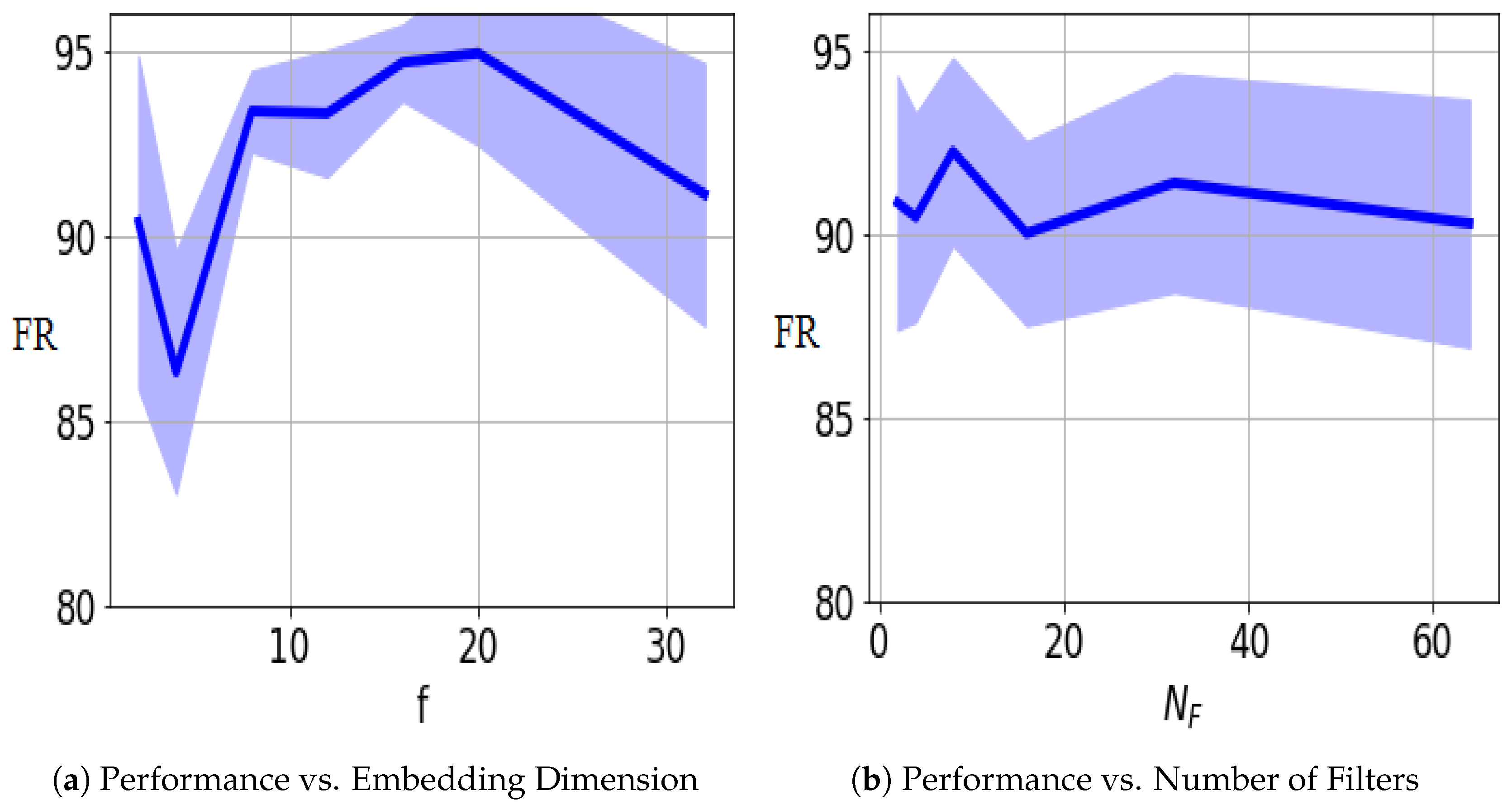
In order to find the optimal parameters for the network structure, we used cross-validation. We first preformed a set of experiments to study empirically the effect of the dimension size (f) of the embedding space on the performance of our algorithm. Figure 2a presents the performance on the SAR testing set versus the dimension of the embedding space when 10 SAR labeled data per class were used for training. The solid line denotes the average performance over ten trials, and the shaded region denotes the standard error deviation. We observed that the performance was quite stable when the embedding space dimension changed. This result suggests that because convolutional layers served to reduce the dimension of input data, if the learned embedding space were discriminative for the source domain, then our method could successfully match the target domain distribution to the source distribution in the embedding. We conclude that for computational efficiency, it is better to select the embedding dimension to be as small as possible. We conclude from Figure 2a that increasing the dimension beyond eight is not helpful. For this reason, we set the dimension of the embedding to be eight for the rest of our experiments in this paper. We performed a similar experiment to investigate the effect of the number of filters on performance. Figure 2b presents the performance on the SAR testing set versus this parameter. We conclude from Figure 2b that is a good choice, as using more filters is not helpful. We did not use a lesser value for to avoid underfitting when the number of labeled data was less than 10.
6.3. Results
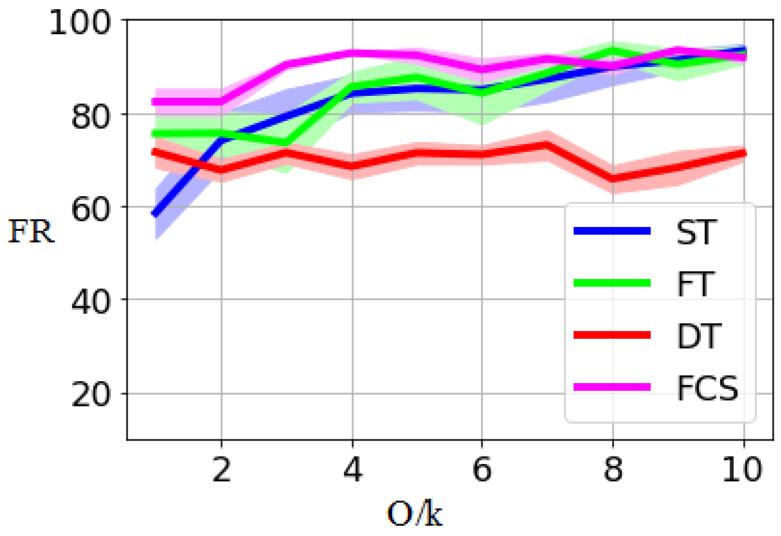
Figure 3 presents the performance results on the data test split for our method along with the three mentioned methods above, versus the number of labeled data points per class that have been used for the SAR domain. For each curve, the solid line denotes the average performance over all ten trials and the shaded region denotes the standard error deviation. These results accord with intuition. It can be seen that direct transfer is the least effective method, as it used no information from the second domain. Supervised training on the SAR domain was not effective in the few-shot learning regime, i.e., its performance was close to chance. The direct transfer method boosted the performance of supervised training in the one-shot regime, but after 2–3 labeled samples per class, as expected, supervised training overtook direct transfer. This was the consequence of using more target task data. In other words, direct transfer only helped to test the network on a better initial point compared to random initialization. Fine-tuning could improve the direct performance, but only for the few-shot regime, and beyond the few-shot learning regime, the performance was similar to supervised training. In comparison, our method outperformed these methods as we benefited from SAR unlabeled data points. For a clearer quantitative comparison, we have presented the data in Figure 3 in Table 1 for different numbers of labeled SAR data points per class (). It is also important to note that in the presence of enough labeled data in the target domain, supervised training would outperform our method because the network was trained using solely the target domain data.
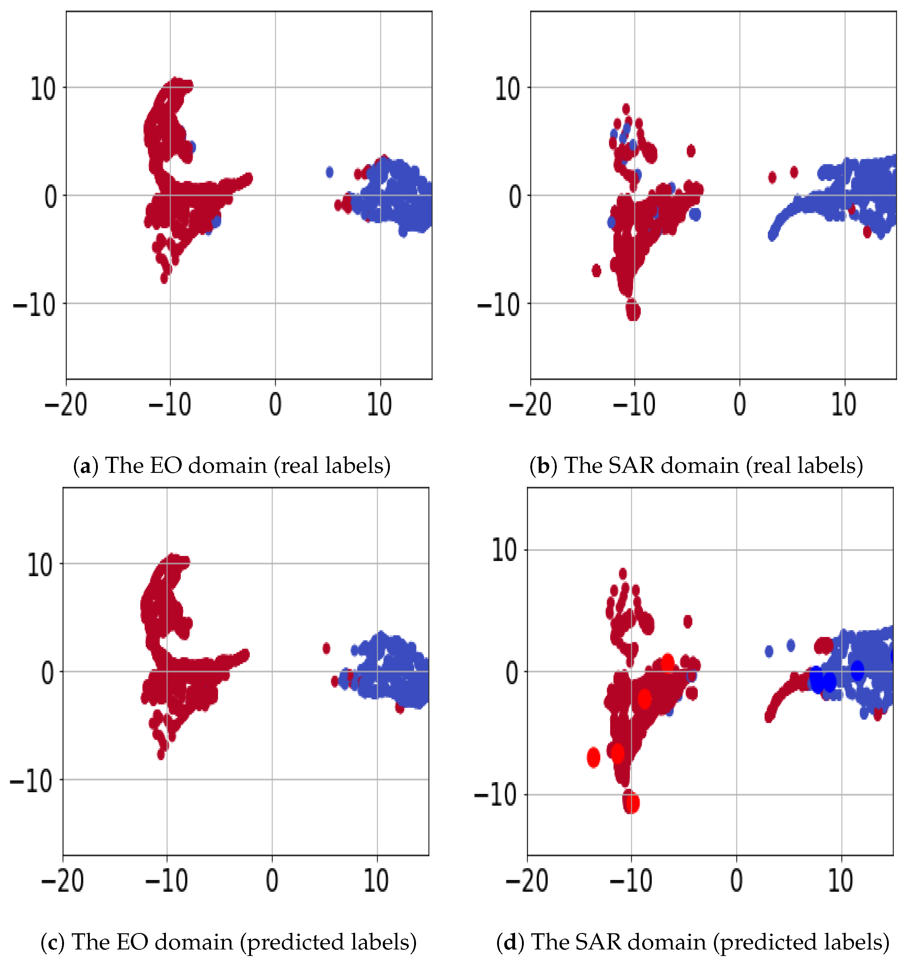
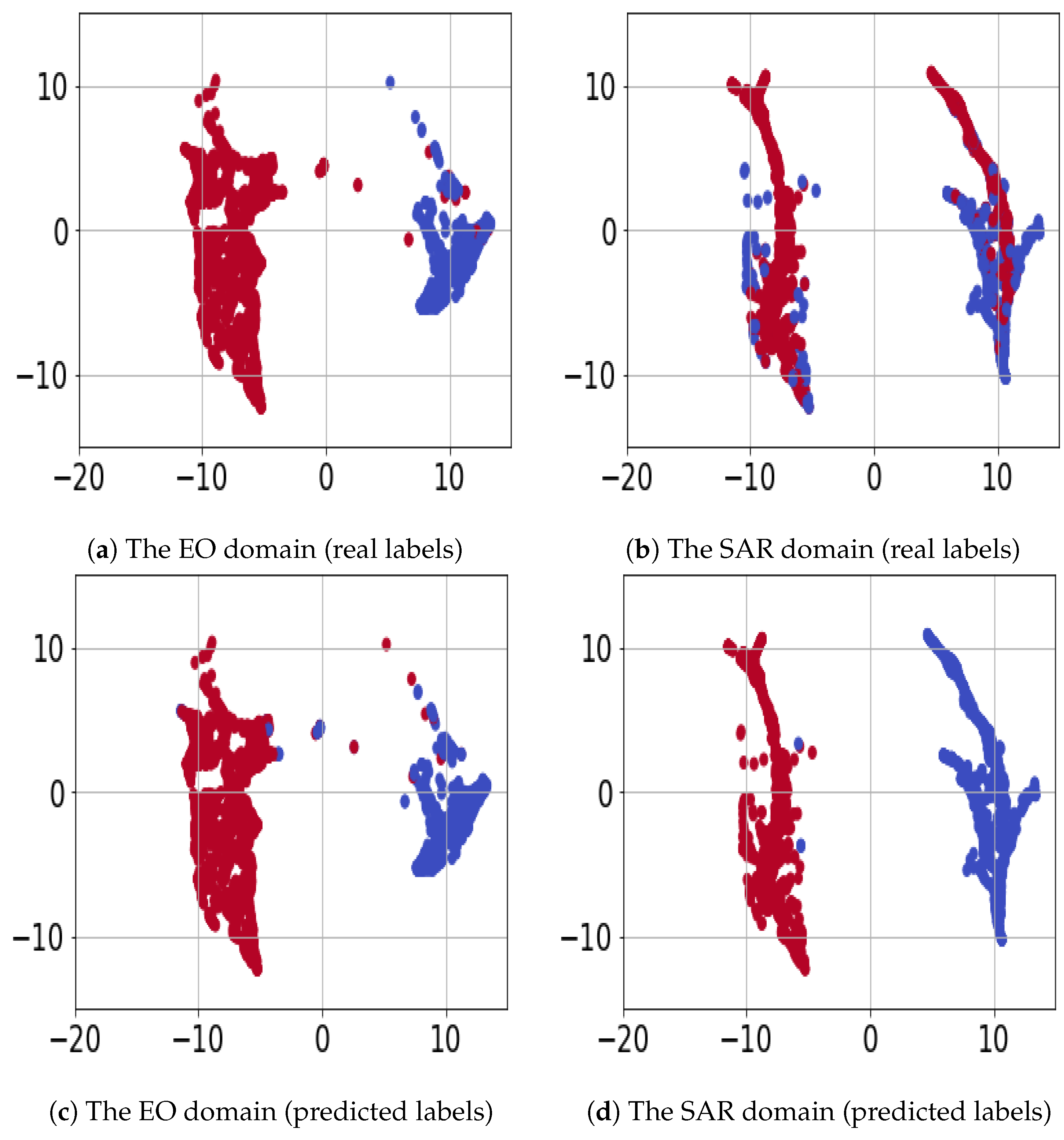
For a better intuition, Figure 4 denotes the Uniform Manifold Approximation and Projection (Umap) visualization [36] of the EO and SAR data points in the learned embedding as the output of the feature extractor encoders. Each point denotes one data point in the embedding that has been mapped to the 2D plane for visualization. In this figure, we have used five labeled data points per class in the SAR domain. In Figure 4, each color corresponds to one of the classes. In Figure 4a,b, we have used real labels for visualization, and in Figure 4c,d, we have used the predicted labels by networks trained using our method for visualization. In Figure 4, the points with brighter red and darker blue colors are the SAR labeled data points that have been used in training. By comparing the top row with the bottom row, we see that the embedding was discriminative for both domains. Additionally, by comparing the left column with the right column, we see that the domain distributions were matched in the embedding class conditionally, suggesting that our framework formulated in Equation (3) was effective. This result suggests that learning an invariant embedding space can serve as a helpful strategy for transferring knowledge. Additionally, we see that labeled data points are important to determine the boundary between two classes, which suggests why part of one of the classes (blue) was predicted mistakenly. This observation suggests that the boundary between classes depends on the labeled target data as the network was certain about the labels of these data points.
We also performed an experiment to serve as an ablation study for our framework. Our previous experiments demonstrated that the first three terms in Equation (3) were all important for successful knowledge transfer. We explained that the fourth term was important for class-conditional alignment. We solved Equation (3) without considering the fourth term to study its effect. We have presented the Umap visualization of the datasets in the embedding space for a particular experiment in Figure 5. We observed that as expected, the embedding was discriminative for the EO dataset, and the predicted labels were close to the real data labels, as the classes were separable. However, despite following a similar marginal distribution in the embedding space, the formed SAR clusters were not class-specific. We can see that in each cluster, we had data points from both classes, and as a result, the SAR classification rate was poor. This result demonstrates that all the terms in Equation (3) were important for the success of our algorithm. We highlight that Figure 5 visualizes the results of a particular experiments, and we observed in some experiments that the classes were matched, even when no labeled target data were used. However, this observations shows that the method is not stable. Using the few labeled data helped to stabilize the algorithm.
7. Conclusions
In this paper, we addressed the problem of SAR image classification when only a few labeled data are available. We formulated this problem as a semi-supervised domain adaption problem. Our idea was based on transferring knowledge from a related electro-optical domain problem where it is easy to generate labeled data. Our classification models were two deep convolutional neural networks that shared their fully-connected layers. The networks were trained such that the convolutional layers served as two deep encoders that matched the distributions of the two EO and SAR domains in an embedding space, which was modeled as their shared output space. We provided a theoretical analysis to explain why our algorithm minimized an upper-bound for the targeted real risk and demonstrated the effectiveness and applicability of our approach for the problem of ship classification in the area of maritime domain awareness. Despite being effective, a major restriction of our method is full overlap between the existing classes across the EO and the SAR domain. A future research direction is to remove this restriction by training the networks such that only the shared classes are matched in the embedding space.
Author Contributions
M.R., S.K., E.E., and K.K. designed the research methodology. M.R. and S.K. validated the ideas and performed software implmentation. M.R., S.K., E.E., and K.K. wrote the paper.
Funding
This research received external funding.
Conflicts of Interest
The authors declare no conflict of interest.
References
- Rostami, M.; Kolouri, S.; Eaton, E.; Kim, K. Explaining distributed neural activations via unsupervised learning. In Proceedings of the IEEE Conference on Computer Vision and Pattern Recognition Workshops, Long Beach, CA, USA, 16–20 June 2019; pp. 20–28. [Google Scholar]
- Koo, V.; Chan, Y.; Vetharatnam, G.; Chua, M.Y.; Lim, C.; Lim, C.; Thum, C.; Lim, T.; bin Ahmad, Z.; Mahmood, K.; et al. A new unmanned aerial vehicle synthetic aperture radar for environmental monitoring. Prog. Electromagn. Res. 2012, 122, 245–268. [Google Scholar] [CrossRef]
- Maitre, H. Processing of Synthetic Aperture Radar (SAR) Images; Wiley: Hoboken, NJ, USA, 2010. [Google Scholar]
- Deng, J.; Dong, W.; Socher, R.; Li, L.J.; Li, K.; Li, F.-F. Imagenet: A large-scale hierarchical image database. In Proceedings of the 2009 IEEE Conference on Computer Vision and Pattern Recognition, Miami, FL, USA, 20–25 June 2009; pp. 248–255. [Google Scholar]
- Rostami, M.; Huber, D.; Lu, T.C. A crowdsourcing triage algorithm for geopolitical event forecasting. In Proceedings of the 12th ACM Conference on Recommender Systems, Vancouver, BC, Canada, 2–7 October 2018; pp. 377–381. [Google Scholar]
- Malmgren-Hansen, D.; Kusk, A.; Dall, J.; Nielsen, A.; Engholm, R.; Skriver, H. Improving SAR automatic target recognition models with transfer learning from simulated data. IEEE Geosci. Remote Sens. Lett. 2017, 14, 1484–1488. [Google Scholar] [CrossRef]
- Schwegmann, C.; Kleynhans, W.; Salmon, B.; Mdakane, L.; Meyer, R. Very deep learning for ship discrimination in synthetic aperture radar imagery. In Proceedings of the IEEE International Geoscience and Remote Sensing Symposium (IGARSS), Beijing, China, 10–15 July 2016; pp. 104–107. [Google Scholar]
- Huang, Z.; Pan, Z.; Lei, B. Transfer learning with deep convolutional neural network for SAR target classification with limited labeled data. Remote Sens. 2017, 9, 907. [Google Scholar] [CrossRef]
- Chen, S.; Wang, H.; Xu, F.; Jin, Y. Target classification using the deep convolutional networks for SAR images. IEEE Trans. Geosci. Remote Sens. 2016, 54, 4806–4817. [Google Scholar] [CrossRef]
- Shang, R.; Wang, J.; Jiao, L.; Stolkin, R.; Hou, B.; Li, Y. SAR Targets Classification Based on Deep Memory Convolution Neural Networks and Transfer Parameters. IEEE J. Sel. Top. Appl. Earth Obs. Remote Sens. 2018, 11, 2834–2846. [Google Scholar] [CrossRef]
- Pan, S.; Yang, Q. A survey on transfer learning. IEEE Trans. Knowl. Data Eng. 2010, 22, 1345–1359. [Google Scholar] [CrossRef]
- Zhang, D.J.; Heng, W.; Ren, K.; Song, J. Transfer Learning with Convolutional Neural Networks for SAR Ship Recognition. IOP Conf. Ser. Mater. Sci. Eng. 2018, 322, 072001. [Google Scholar] [CrossRef]
- Wang, Z.; Du, L.; Mao, J.; Liu, B.; Yang, D. SAR Target Detection Based on SSD With Data Augmentation and Transfer Learning. IEEE Geosci. Remote Sens. Lett. 2019, 16, 150–154. [Google Scholar] [CrossRef]
- Lang, H.; Wu, S.; Xu, Y. Ship classification in SAR images improved by AIS knowledge transfer. IEEE Geosci. Remote Sens. Lett. 2018, 15, 439–443. [Google Scholar] [CrossRef]
- Motiian, S.; Jones, Q.; Iranmanesh, S.; Doretto, G. Few-shot adversarial domain adaptation. Adv. Neural Inf. Process. Syst. 2017, 6670–6680. [Google Scholar]
- Redko, I.; Habrard, A.; Sebban, M. Theoretical analysis of domain adaptation with optimal transport. In Joint European Conference on Machine Learning and Knowledge Discovery in Databases; Springer: Cham, Switzerland, 2017; pp. 737–753. [Google Scholar]
- Villani, C. Optimal Transport: Old and New; Springer Science & Business Media: Berlin/Heidelberg, Germany, 2008; Volume 338. [Google Scholar]
- Gretton, A.; Smola, A.; Huang, J.; Schmittfull, M.; Borgwardt, K.; Schölkopf, B. Covariate shift by kernel mean matching. In Dataset Shift in Machine Learning; The MIT Press: Cambridge, MA, USA, 2009. [Google Scholar]
- Rabin, J.; Peyré, G.; Delon, J.; Bernot, M. Wasserstein barycenter and its application to texture mixing. In International Conference on Scale Space and Variational Methods in Computer Vision; Springer: Berlin/Heidelberg, Germany, 2011; pp. 435–446. [Google Scholar]
- Kolouri, S.; Rohde, G.K.; Hoffman, H. Sliced Wasserstein Distance for Learning Gaussian Mixture Models. In Proceedings of the IEEE Conference on Computer Vision and Pattern Recognition, Salt Lake City, UT, USA, 18–22 June 2018; pp. 3427–3436. [Google Scholar]
- Kodirov, E.; Xiang, T.; Fu, Z.; Gong, S. Unsupervised domain adaptation for zero-shot learning. In Proceedings of the IEEE International Conference on Computer Vision, Santiago, Chile, 7–13 December 2015; pp. 2452–2460. [Google Scholar]
- Goodfellow, I.; Pouget-Abadie, J.; Mirza, M.; Xu, B.; Warde-Farley, D.; Ozair, S.; Courville, A.; Bengio, Y. Generative adversarial nets. In Proceedings of the Advances in Neural Information Processing Systems 27 (NIPS 2014), Montreal, QC, Canada, 8–13 December 2014; pp. 2672–2680. [Google Scholar]
- Courty, N.; Flamary, R.; Tuia, D.; Rakotomamonjy, A. Optimal transport for domain adaptation. IEEE TPAMI 2017, 39, 1853–1865. [Google Scholar] [CrossRef] [PubMed]
- Daume, H., III; Marcu, D. Domain adaptation for statistical classifiers. J. Artif. Intell. Res. 2006, 26, 101–126. [Google Scholar] [CrossRef]
- Kolouri, S.; Pope, P.E.; Martin, C.E.; Rohde, G.K. Sliced-Wasserstein Auto-Encoders. In Proceedings of the International Conference on Learning Representation (ICLR), New Orleans, LA, USA, 6–9 May 2019. [Google Scholar]
- Bonneel, N.; Rabin, J.; Peyré, G.; Pfister, H. Sliced and Radon Wasserstein barycenters of measures. J. Math. Imaging Vis. 2015, 51, 22–45. [Google Scholar] [CrossRef]
- Carriere, M.; Cuturi, M.; Oudot, S. Sliced wasserstein kernel for persistence diagrams. arXiv 2017, arXiv:1706.03358. [Google Scholar]
- Long, M.; Wang, J.; Ding, G.; Sun, J.; Yu, P.S. Transfer joint matching for unsupervised domain adaptation. In Proceedings of the IEEE Conference on Computer Vision and Pattern Recognition, Portland, OR, USA, 23–28 June 2014; pp. 1410–1417. [Google Scholar]
- Damodaran, B.; Kellenberger, B.; Flamary, R.; Tuia, D.; Courty, N. DeepJDOT: Deep Joint distribution optimal transport for unsupervised domain adaptation. arXiv 2018, arXiv:1803.10081. [Google Scholar]
- Kolouri, S.; Park, S.R.; Thorpe, M.; Slepcev, D.; Rohde, G.K. Optimal Mass Transport: Signal processing and machine-learning applications. IEEE Signal Process. Mag. 2017, 34, 43–59. [Google Scholar] [CrossRef] [PubMed]
- Bonnotte, N. Unidimensional and Evolution Methods for Optimal Transportation. Ph.D. Thesis, Scuola Normale Superiore, Paris, France, 2013. [Google Scholar]
- Santambrogio, F. Optimal Transport for Applied Mathematicians; Birkäuser: New York, NY, USA, 2015; pp. 99–102. [Google Scholar]
- Schwegmann, C.P.; Kleynhans, W.; Salmon, B.P.; Mdakane, L.W.; Meyer, R.G.V. A SAR Ship Dataset for Detection, Discrimination and Analysis. Data Retrieved from Kaggle. 2017. Available online: https://ieee-dataport.org/documents/sar-ship-dataset-detection-discrimination-and-analysis (accessed on 1 February 2019).
- Hammell, R. Ships in Satellite Imagery. Data Retrieved from Kaggle. 2017. Available online: https://www.kaggle.com/rhammell/ships-in-satellite-imagery (accessed on 1 February 2019).
- Kingma, D.P.; Ba, J. Adam: A method for stochastic optimization. arXiv 2014, arXiv:1412.6980. [Google Scholar]
- McInnes, L.; Healy, J.; Melville, J. Umap: Uniform manifold approximation and projection for dimension reduction. arXiv 2018, arXiv:1802.03426. [Google Scholar]
Figure 1.
Block diagram architecture of the proposed framework for transferring knowledge from the Electro-Optical (EO) to the SAR domain.
Figure 1.
Block diagram architecture of the proposed framework for transferring knowledge from the Electro-Optical (EO) to the SAR domain.

Figure 2.
The SAR test performance versus the dimension of the embedding space and the number of filters.
Figure 2.
The SAR test performance versus the dimension of the embedding space and the number of filters.

Figure 3.
The SAR test performance versus the number of labeled data per class. ST, Supervised Training; FT, Fine-Tuning; DT, Direct Transfer.
Figure 3.
The SAR test performance versus the number of labeled data per class. ST, Supervised Training; FT, Fine-Tuning; DT, Direct Transfer.

Figure 4.
Umapvisualization of the EO versus the SAR dataset in the shared embedding space (view in color).
Figure 4.
Umapvisualization of the EO versus the SAR dataset in the shared embedding space (view in color).

Figure 5.
Umap visualization of the EO versus the SAR dataset for the ablation study (view in color).
Figure 5.
Umap visualization of the EO versus the SAR dataset for the ablation study (view in color).


Table 1.
Comparison results for the SAR test performance.
| 1 | 2 | 3 | 4 | 5 | 6 | 7 | |
|---|---|---|---|---|---|---|---|
| ST | 58.5 | 74.0 | 79.2 | 84.1 | 85.2 | 84.9 | 87.2 |
| FT | 75.5 | 75.6 | 73.5 | 85.5 | 87.6 | 84.2 | 88.5 |
| DT | 71.5 | 67.6 | 71.4 | 68.5 | 71.4 | 71.0 | 73.1 |
| FCS | 86.3 | 86.3 | 82.8 | 94.2 | 87.8 | 96.0 | 91.1 |
© 2019 by the authors. Licensee MDPI, Basel, Switzerland. This article is an open access article distributed under the terms and conditions of the Creative Commons Attribution (CC BY) license (http://creativecommons.org/licenses/by/4.0/).
Share and Cite
MDPI and ACS Style
Rostami, M.; Kolouri, S.; Eaton, E.; Kim, K. Deep Transfer Learning for Few-Shot SAR Image Classification. Remote Sens. 2019, 11, 1374. https://0-doi-org.brum.beds.ac.uk/10.3390/rs11111374
AMA Style
Rostami M, Kolouri S, Eaton E, Kim K. Deep Transfer Learning for Few-Shot SAR Image Classification. Remote Sensing. 2019; 11(11):1374. https://0-doi-org.brum.beds.ac.uk/10.3390/rs11111374
Chicago/Turabian StyleRostami, Mohammad, Soheil Kolouri, Eric Eaton, and Kyungnam Kim. 2019. "Deep Transfer Learning for Few-Shot SAR Image Classification" Remote Sensing 11, no. 11: 1374. https://0-doi-org.brum.beds.ac.uk/10.3390/rs11111374
Note that from the first issue of 2016, this journal uses article numbers instead of page numbers. See further details here.