Article

An Automated Python Language-Based Tool for Creating Absence Samples in Groundwater Potential Mapping

1
Geographic Information Science Research Group, Ton Duc Thang University, Ho Chi Minh City 70000, Viet Nam
2
Faculty of Environment and Labour Safety, Ton Duc Thang University, Ho Chi Minh City 70000, Viet Nam
3
Department of Watershed Management, Faculty of Agriculture and Natural Resources, Lorestan University, Khorramabad 68151-44316, Iran
4
Department of Watershed Management Engineering, Faculty of Natural Resources, Tarbiat Modares University, Tehran 46417-76489, Iran
5
Department of Physical Geography and Bolin Centre for Climate Research, Stockholm University, SE-106 91 Stockholm, Sweden
6
Faculty of Natural Resources, University of Tehran, Karaj 31587-77871, Iran
7
Division of Geoscience Research Platform, Korea Institute of Geoscience and Mineral Resources (KIGAM), 124 Gwahang-no, Yuseong-gu, Daejeon 305-350, Korea
8
Institute of Research and Development, Duy Tan University, Da Nang 550000, Viet Nam
*
Authors to whom correspondence should be addressed.
Remote Sens. 2019, 11(11), 1375; https://0-doi-org.brum.beds.ac.uk/10.3390/rs11111375
Submission received: 2 May 2019 / Revised: 30 May 2019 / Accepted: 5 June 2019 / Published: 9 June 2019

Abstract

:
Although sampling strategy plays an important role in groundwater potential mapping and significantly influences model accuracy, researchers often apply a simple random sampling method to determine absence (non-occurrence) samples. In this study, an automated, user-friendly geographic information system (GIS)-based tool, selection of absence samples (SAS), was developed using the Python programming language. The SAS tool takes into account different geospatial concepts, including nearest neighbor (NN) and hotspot analyses. In a case study, it was successfully applied to the Bojnourd watershed, Iran, together with two machine learning models (random forest (RF) and multivariate adaptive regression splines (MARS)) with GIS and remotely sensed data, to model groundwater potential. Different evaluation criteria (area under the receiver operating characteristic curve (AUC-ROC), true skill statistic (TSS), efficiency (E), false positive rate (FPR), true positive rate (TPR), true negative rate (TNR), and false negative rate (FNR)) were used to scrutinize model performance. Two absence sample types were produced, based on a simple random method and the SAS tool, and used in the models. The results demonstrated that both RF (AUC-ROC = 0.913, TSS = 0.72, E = 0.926) and MARS (AUC-ROC = 0.889, TSS = 0.705, E = 0.90) performed better when using absence samples generated by the SAS tool, indicating that this tool is capable of producing trustworthy absence samples to improve groundwater potential models.

Graphical Abstract

1. Introduction

Different approaches such as data-driven, statistical, and machine learning models can be used to model groundwater potential. They are based on a statistical assumption that the past and present situations and state of a phenomenon are key to determining and predicting its future situation and state. The models use two different data samples as the dependent variable: occurrence samples (also known as presence or positive samples) and non-occurrence samples (also known as absence or negative samples) [1,2]. Beside the dependent variable, different geo-environmental factors are considered as independent variables. In other words, the spatial modeling approach requires an inventory of occurrences and non-occurrences and a set of geo-environmental attributes related to groundwater spring [3,4]. Presence samples are usually obtained by conducting field surveys and analyses of high-quality aerial photographs and satellite images. They are thus usually more reliable than absence samples, because they are based on proof of existence of the given phenomenon. Absence samples are typically selected as individual pixels outside the occurrence areas (i.e., spring-free areas), using a simple random sampling method [5,6]. Therefore, determining absence samples (i.e., non-spring) is usually a challenging task and can be a key source of model uncertainty, strongly affecting model performance [7,8].
The quality of both presence and absence samples is extremely important in the modeling process because any error in selection of these samples can lead to a significant error in the final modeling or analysis process. Generally, two main errors can arise in the modeling results: Type I error and Type II error [9]. Considering the example of landslide susceptibility, Type I error, also called ‘false positive’, indicates areas without risk being classified as unsafe. This error may lead to exclusion of these areas from development plans and cause many social and economic problems. On the other hand, Type II errors, called ‘false negative’, involve areas that are unsafe being classified as safe. This error can cause some severe problems in the real world, such as economic damage and loss of life, since using maps produced with Type II error can lead to structures or developments being placed in areas that are unstable or unsafe [9]. Both presence and absence samples strongly influence these error types and, consequently, the predictive performance of the model [10,11]. A performance improvement of only a few percent can lead to more efficient water resources and environmental management [12]. Therefore, powerful standard approaches are required to select absence and presence samples with high accuracy.
Because of lack of reasonable and trustworthy techniques, most spatial modeling studies reported in the literature use a simple random method to select absence samples in different fields, for example, groundwater potential [3,5,10,13,14,15,16], landslide susceptibility [1,17,18,19,20,21], gully erosion susceptibility [22,23,24,25], land subsidence susceptibility [26,27,28,29,30,31], and flood susceptibility [18,32,33,34,35,36,37]. However, the random sampling method has some drawbacks. First, this method does not pay attention to the distribution pattern of absence samples, and therefore the absence samples generated are sometimes significantly clustered and do not provide overall information on the entire study area [34,38]. Second, absence samples may be very close to presence locations, resulting in confusion in the model and also increasing an error in the final output [39]. It is important that absence samples are selected from areas that are reasonably far from the area of the presence samples. Therefore, studies should seek to systematically reduce uncertainties associated with absence samples.
In light of these problems, it is necessary to develop a robust novel tool for selecting absence samples with high accuracy and precision. The main objectives of the present study were thus to: (1) develop an automated, user-friendly tool for selection of absence samples using the Python programming language to select absence samples; (2) apply the selected absence samples in two different machine learning models, random forest (RF) and multivariate adaptive regression splines (MARS), to analyze groundwater potential; (3) evaluate the model accuracy using two common statistical methods; and (4) compare the results of models using absence samples generated by the SAS tool and by a simple random method. The RF and MARS models were chosen because they have been commonly used by different scholars for groundwater potential mapping and their capabilities have been proven [3,10,15,40,41]. This allowed us to investigate only the efficiency of the developed tool, selection of absence samples (SAS). Another reason for selecting these two models is that in terms of model structure they are very different. It should be pointed out that there are a number of other machine learning models, but comparison of their performance was outside the scope of this paper. The novel feature of this study was to develop a suitable framework for selecting absence samples and statistically comparing their performances against those of the ordinary random methods used by previous researchers.

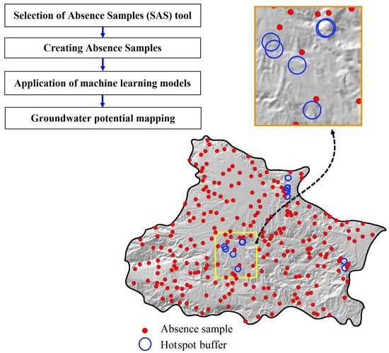
2. Development of the SAS Tool

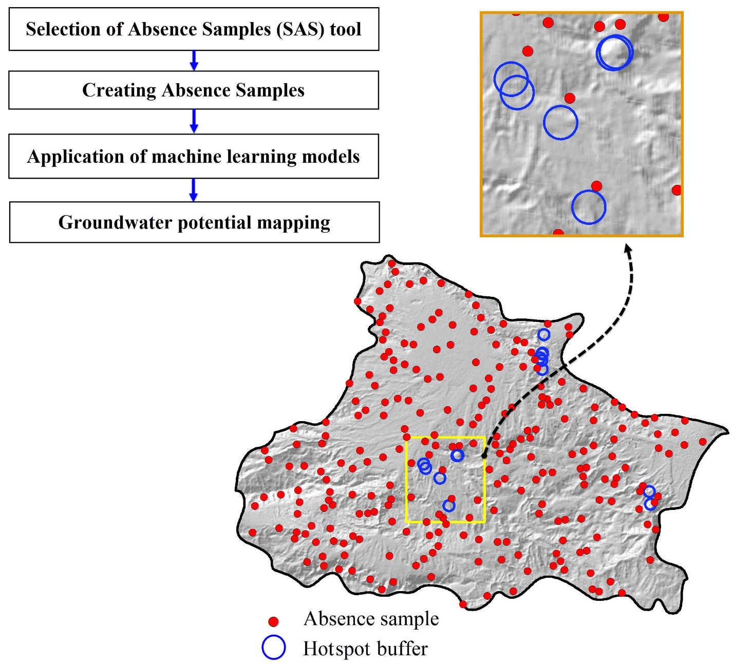
2.1. Technical Background

In order to create a robust absence sample dataset, different precondition analyses were considered. The conceptual architecture of our approach for selection of absence samples (the SAS tool) is illustrated in Figure 1. In the following subsections, the three-step process is explained in detail.
Step 1: Determining a buffer for presence samples
One of the main problems with selecting absence samples based on a random paradigm is that the absence samples selected may be at or very close to presence samples, which can cause different errors in the model results. In the random sampling method, absence and presence samples may be selected from regions with completely similar properties in which the triggering factors are in a similar condition. Consequently, the modeling approach may encounter a serious misunderstanding about the related process. Therefore, the first step in the SAS tool is to create a buffer zone around the presence samples. This method has been used previously to define absence samples for landslide susceptibility mapping by extracting absence samples from randomly distributed circles [7]. This buffer causes the absence and presence samples to be selected reasonably far from each other. In the SAS tool, the radius of the buffer can be determined by the user and depends on the nature of the phenomenon under study.
Step 2: Average nearest neighbor
Another important issue in absence sample selection is their distribution in the study area. An efficient method for determining the distribution pattern of samples is the average nearest neighbor (NN) approach [42,43]. This algorithm measures the distance between the centroid of each object and the centroid of its nearest neighbor using a nearest neighbor index. The average of all these nearest neighbor distances is then calculated. An average nearest neighbor ratio less than 1 indicates that the samples are clustered, while an average nearest neighbor ratio greater than 1 indicates dispersion of samples [44,45]. This algorithm compares average distance with average distance for a hypothetical random distribution. The nearest neighbor (NN) index is calculated as [41]:
N N = D ¯ O D ¯ E
where D ¯ O is the observed mean distance between each feature and its nearest neighbor, calculated using Equation (2), and D ¯ E is the expected mean distance for a hypothetical random distribution, calculated using Equation (3) [41]:
D ¯ O = i = 1 n d i n
D ¯ E = 0.5 n A
where di equals the distance between feature i and its nearest neighboring feature, n corresponds to the total number of features, and A is the area of a minimum enclosing rectangle around all features or a user-specified area value. The average nearest neighbor z-score can be also calculated as:
z = D ¯ O D ¯ E S E
where   S E = 0.26136 n 2 A
Figure 2 shows a schematic illustration of the relationship between distribution pattern of samples and NN index. As can be seen, low values of NN index correspond to a clustered distribution and high values of NN index correspond to a dispersed distribution of samples [46,47].
Step 3: Hotspot analysis (Getis-Ord Gi*)
Hotspot analysis is an efficient way to calculate the Getis-Ord Gi* statistic, which indicates where features cluster spatially [48]. This algorithm considers an object or feature related to its neighboring features. A feature is only considered a significant hotspot when it has a high value and is also surrounded by other features with high values [49]. In this way, the local sum for each feature and its neighbors is calculated. This local sum is then compared against the sum of all features. If the local sum is considerably greater than the estimated local sum and cannot have resulted from random chance, it can be considered a significant hotspot [46,50]. In this study, hotspot analysis was carried out using the Getis-Ord Gi* statistic for each sample in the presence inventory, calculated as [51]:
G i * = j = 1 n w i , j x j X ¯ j = 1 n w i , j S [ n j = 1 n w i , j 2 ( j = 1 n w i , j ) 2 ] n 1
where xj is the attribute value for feature j, wi,j is the spatial weight between feature i and j, n is equal to the total number of features, and:
X ¯ = j = 1 n x j n
S = j = 1 n x j 2 n ( X ¯ ) 2
Figure 3 shows a schematic diagram of hotspot analysis. As can be seen in the diagram, there are some points with high values that are not considered hotspots, because the surrounding features have low values [20]. Hotspot areas not only include presence samples with high values, but all samples in these areas are also characterized by high values. Hotspot samples with high values, where the surrounding objects also have high values, are shown in red in Figure 3.

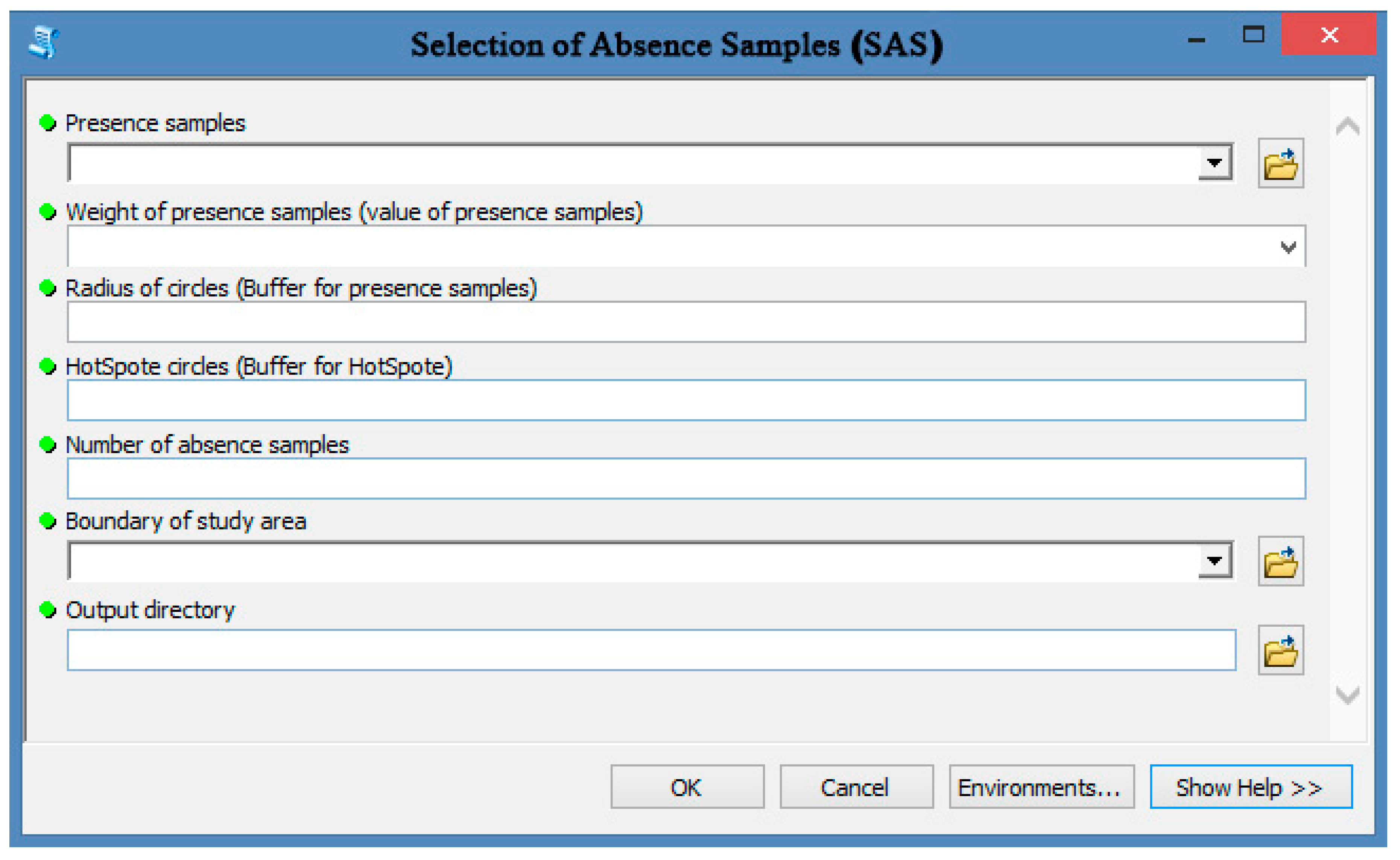
2.2. Designing the SAS Tool

The SAS tool was developed using Python, a powerful, high-level, object-oriented, and structured general-purpose programming language. The ArcPy library, which builds on the successful ArcGIS scripting module, was used in this study. Using this programming language, an extension was provided that can be added to the Arctoolbox in the ArcGIS software. The main SAS tool coding and structure design tasks were to develop an automated procedure for generating absence samples that met the three technical conditions described in Section 2.1.
A view of the SAS tool and its components is presented in Figure 4. As can be seen, this tool has several different parts, including inputs and outputs. Table 1 lists the SAS input parameters and files. In the first part, the presence samples layer is imported by the user. These presence samples (positive points) are the location of occurrences for a given phenomenon in shape file format. This layer can be produced using inventory maps, aerial photographs, satellite images, or field surveys. An example is the location of springs in a specific region. The next part is to assign a value (weight) to the presence samples. Here, the user must define the field that includes values related to the presence samples. For example, the amount of discharge from springs can be imported in this input parameter. Another input parameter in the SAS tool is the radius of circles or the buffer for presence samples. This radius value determines the buffer zone in which absence samples cannot be created. After hotspot samples are calculated, hotspot buffers should be produced for each. As done for the presence samples, the user must determine a buffer zone for the hotspot points. Number of absence samples can be determined in the next field. Generally, the number of absence samples should be equal to the number of presence samples. Finally, the SAS tool needs a boundary of the study area. This boundary helps the tool to determine the permitted sites for producing absence samples.
The SAS tool provides three main outputs, which are listed in Table 2. The first output is the absence samples layer, which contains the locations of the absence samples. These samples are selected according to the buffer of presence samples, average nearest neighbor, and hotspot analyses. The second main output of the SAS tool is the ‘hotspot and coldspot’ layer, where SAS classifies the presence samples into three classes, namely coldspot, medium, and hotspot, according to their values. The final output is the significance information from hotspot analysis, which shows presence samples that are significant hotspots in comparison with other presence samples. It is worth mentioning that the aim of the SAS tool is simply to produce an absence sample layer. However, the results of hotspot analysis on presence samples can provide useful information, and therefore we retain them as one of the main model outputs.

3. Case Study

In a case study, the SAS tool was applied to generate an absence sample layer for the Bojnourd watershed, North Khorasan province, Iran (37°15′–37°35′ N, 57°03′–57°40′ E) (Figure 5). The aim in the case study was to model groundwater potential, and an absence sample layer was needed, while presence samples (i.e., groundwater springs) were readily available, as shown in Figure 5. The elevation of the study area ranges between 875 and 2968 m, mean annual precipitation is 272 mm, and mean annual temperature is 13 °C (Khorasan Shomali Meteorological Organization). Groundwater is one of the main water resources in the area. From a geomorphological viewpoint, the region is classified as mountainous and there are several faults and folds that play a significant role in the development of springs. North Khorasan province has around 17,000 km2 of karst masses, which supply around 88% of the water demand in the province.

3.1. Application of the SAS Tool

Both the simple random sampling method and the newly developed SAS tool were used to produce absence samples in order to model groundwater potential in the study area. The absence samples generated using the common random method are shown in Figure 6a, and those produced using the SAS tool are shown in Figure 6b. In order to highlight the difference between the random method and the SAS tool, the absence samples they produced are overlaid (Figure 6). In the diagrams, blue circles represent the hotspot buffers and red points the absence samples. As can be seen in the zoomed-in parts of the map, the simple random method created several absence samples that were very close to each other (i.e., had a clustered distribution pattern) and also fell within the hotspot buffers (i.e., blue circles). In contrast, the SAS method created absence samples that were reasonably far from each other (i.e., had a dispersed distribution pattern) and, more importantly, that did not fall within the hotspot buffers. Moreover, with the use of the random method, several parts of the study area had no absence samples, while numerous absence samples were unreasonably concentrated in some other parts. In contrast, the SAS tool met all three preconditions (no absence samples on or near presence samples, dispersed absence samples, no absence samples in hotspot buffers). Therefore, the method used for selection of absence samples had a considerable influence on the absence samples.

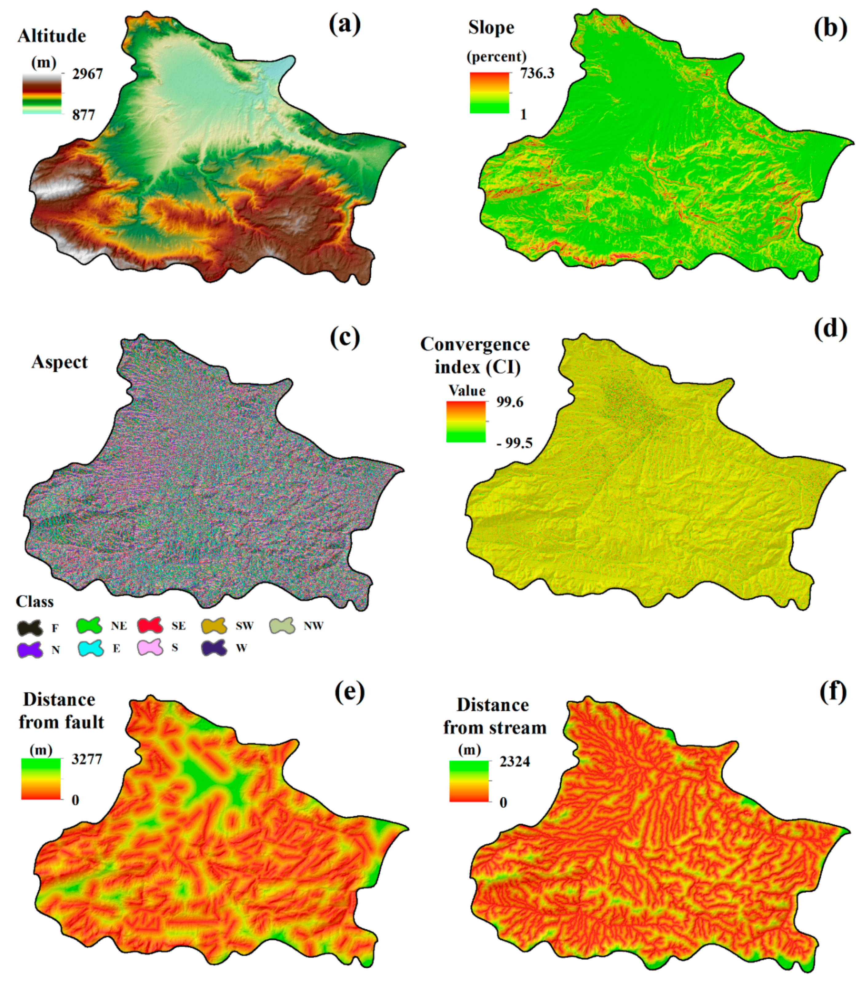
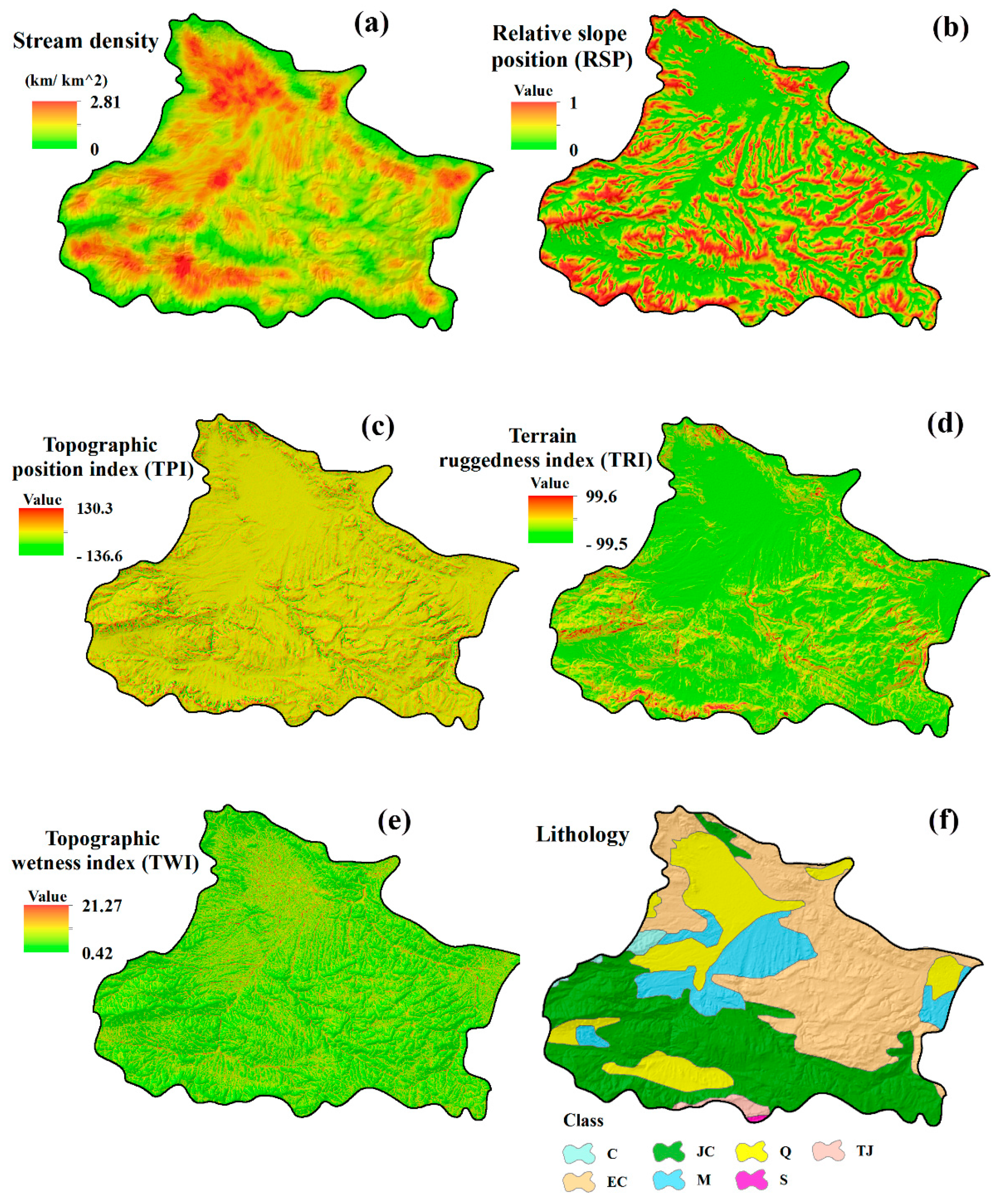
3.2. Groundwater-Affecting Factors

Groundwater-affecting factors (GAFs) contribute in the modeling process as independent variables. Since there are no universal guidelines for selecting GAFs, previous studies have considered different geo-environmental and topo-hydrological factors [43,52,53]. Based on the literature, sixteen GAFs were selected in the present study to spatially predict groundwater spring potential. These were altitude, slope, aspect, profile curvature, plan curvature, land use/cover, lithology, soil, distance from fault, distance from stream, stream density, relative slope position (RSP), topographic wetness index (TWI), topographic position index (TPI), terrain roughness index (TRI), and convergence index (CI) (Figure 7 and Figure 8).
Both remote sensing and geographical information system (GIS) techniques were used to produce groundwater-affecting factors. First, a digital elevation model (DEM) was produced using the airborne LIDAR (light detection and ranging) system, which is an effective and reliable means of collecting topographical data in large areas. The triangular irregular network (TIN) generated was converted to an ArcGIS grid of 1 m pixel resolution using a TOPOGRID algorithm. In order to achieve homogeneity with other predictive maps and to increase efficiency in terms of manipulation and storage, the high-resolution DEM produced was coarsened to 10 m resolution. This resolution was considered to create topography-related predictive factors, including altitude, slope, aspect, profile curvature, plan curvature, distance from fault, distance from stream, stream density, RSP, TWI, TPI, TRI, and CI. In addition, in order to create an accurate land use map, Landsat-8 Operational Land Imager (OLI) images in 2018 were used. Atmospheric corrections were performed using the FLAASH module in ENVI software. Next, the Gram-Schmidt pan-sharpening module was used for the fusion of panchromatic and multispectral satellite images. In addition, a supervised classification approach with the maximum likelihood algorithm was carried out. Finally, in accordance with the resolution of other DEM-extracted factors, the land use map produced was resampled with a spatial resolution of 10 m in ENVI software.
Altitude in the study area varies from 877 to 2967 m. A slope map with range from 1% to 736.3% was produced using the DEM generated. The slope aspect classes are shown in Figure 7c. The CI is a terrain parameter that reflects the structure of the relief as a set of divergent areas (ridges) and convergent areas (channels). If the CI value is positive, then the pixel is defined as divergent, while convergent pixels have a negative CI [54,55]. In this study, the CI map was produced in SAGA (System for Automated Geoscientific Analyses) software and the CI value ranged from −99.5 to 99.6 (Figure 7d). The minimum and the maximum ‘distance from fault’ values were calculated to be 0 and 3277 m, respectively (Figure 7e). ‘Distance from streams’ values calculated for the study area varied between 0 and 2324 m (Figure 7f). To analyze the stream density in the study, the Kernel density tool was used. The minimum and maximum stream density values in the study area were 0 and 2.8, respectively (Figure 8a). The RSP map was generated in SAGA software, and its values ranged from 0 to 1 (Figure 8b). TPI measures the difference between elevation at the central point and average elevation around it within a predetermined radius [11]. Negative TPI values show that the central point is located lower than its average surroundings, while positive values indicate a position higher than the average. In this study, TPI values varied between −136.6 and 130.3 (Figure 8c). TRI, produced in SAGA software, was also used as a measurement of terrain heterogeneity. It ranged from −99.5 to 99.6 in the study area (Figure 8d). TWI is one of the secondary topographic factors and is calculated based on the specific catchment area and the local slope. TWI is a relative measure of the soil moisture availability of a given site in the watershed [56]. TWI values ranged from 0.42 to 21.27 in the study area, which indicates significant variation in spatial patterns of saturated areas (Figure 8e). A lithological map of the study area was digitized from a geological map of Khorasan province published by the Geological Survey of Iran (GSI) (Figure 8f). A detailed description of lithological classes can be found in Table 3.

3.3. Groundwater Potential Modeling

In this study, two state-of-the-art machine learning models, RF and MARS, were used to model groundwater potential, due to their structural flexibility. In the modeling process, two different absence sample types were used: (1) those produced by the simple random method, and (2) those produced by the SAS method (i.e., meeting all three preconditions).

3.3.1. Random Forest (RF)

Random Forest is a non-parametric model introduced as a form of classification and regression tree method [57]. It consists of a combination of tree classifiers, where each tree is created using a random vector sampled independently from the input vector. To classify an input vector, each tree also casts a unit vote for the most popular class. The combination of several classification trees in a forest can improve the performance of predictions. In this approach, a randomized subgroup of variables of interest is used to split the tree, and the average of all tree results is considered the final outcome of the model [53,58]. The random selection of features at each node reduces the correlation between the trees in the forest, thus decreasing the forest error rate. In addition to random feature selection, averaging over numerous trees can also decrease bias and variance [59]. Additionally, RF has vigorous error estimates and higher prediction performance. Other characteristics of RF are random feature selection at each node and a no pruning or stopping rule [60]. Through these, overfitting is significantly reduced. In the RF model, bootstrap samples are used to produce trees. The RF approach rests upon the basic premise that a set of classification trees has better performance than a stand-alone classifier. It has the following advantages [40,53,61]:
  • it is relatively robust to noise and outliers;
  • it provides an internal unbiased estimate of the generalization error through out-of-bag (OOB) error;
  • it estimates the importance of variables in the modeling process (i.e., contribution of variables);
  • it can handle numerous input variables (i.e., predictive factors) without variable deletion;
  • it efficiently handles large databases; and
  • it reduces the computational burden and is computationally lighter than other tree-based models.
In general, design of a tree-based model requires a pruning method and the choice of an attribute selection measure. The Gini index and the information gain ratio are the most frequently used attribute selection measures in tree-based models. RF uses the Gini index to measure the impurity of an attribute. The Gini index allows selection of the split with the lowest impurity at each node [61]. Among the trees in the forest, the class with the maximum number of votes is the predicted class of an observation. In this study, the RF model was implemented using the package ‘randomforest’ in R software.

3.3.2. Multivariate Adaptive Regression Splines (MARS)

The MARS model is a non-parametric form of regression analysis [62]. It combines the mathematical construction of splines, classical linear regression, brute search intelligent algorithms, and binary recursive partitioning to develop a model capable of predicting a target variable [63]. Since MARS uses piecewise basis functions, it can model complex relationships between variables without strong model assumptions. MARS considers each sample as a knot and develops a linear regression model with the candidate feature(s). When implementing a MARS model, knots are selected automatically in a forward stepwise manner. The knot is a key concept in the MARS model and characterizes a point where the behavior of the function changes. In order to define a set of piecewise functions (also known as basic functions, BFs), candidate knots can be placed at any position within the range of each independent variable. In fact, the beginning and end of each BF is determined by a knot. The MARS model selects the knot and its corresponding pair of basic functions at each step, which can significantly decrease the residual sum of squares [64]. The search lasts until all possible BFs have been found. The least important BF is identified and eliminated. Similar to the RF model, MARS is able to analyze the importance of variables and this characteristic is very useful, especially when some potential or new variables are considered. In addition, MARS can save much modeling time when the dataset is huge, because it does not need a long training process [65,66]. It also searches for potential interactions between predictive variables, allowing any degree of interaction to be analyzed in the model building process. Through these characteristics, MARS is able to yield homogeneous final groups in the terminal nodes and minimize prediction errors [67]. In addition, it allows the contribution of predictive variables to be assessed using the generalized cross-validation criterion [66]. The MARS model can be described as follows:
Y = β 0 + m = 1 M β m h m ( x )
where Y is the value predicted by the model and can be decomposed into a sum of M terms (each of which is formed by a coefficient βm and BF hm(x)) and an initial constant β0. Detailed background and characteristics of the MARS model can be found in [62]. Therefore, it has considerable advantages in modeling natural processes in data-scarce regions. In this study, the MARS model was implemented using the package ‘earth’ in R software.

3.4. Accuracy Assessment

In order to evaluate the accuracy of the models, a threshold-dependent method (area under the receiver operating characteristic curve, AUC-ROC) and different threshold-independent methods (false positive rate (FPR), true positive rate (TPR), true negative rate (TNR), false negative rate (FNR), the true skill statistic (TSS), and efficiency (E)) [68,69] were used in this study. FPR estimates the probability of incorrectly predicting a non-occurrence location as an occurrence. TPR, also known as sensitivity, indicates the probability of correctly predicting the positives as observed in reality. However, FPR and TPR are insufficient performance metrics, because they ignore false negatives and false positives, respectively [9]. TNR aims to quantify the probability of correctly predicting the negatives as they occur in reality. Furthermore, FNR, also termed miss rate, determines the probability of incorrectly predicting an occurrence location as a non-occurrence. TSS (also called Pierce’s skill score) measures the ability of a predicted value to discriminate between occurrence and non-occurrence. Although researchers have used the kappa coefficient to evaluate model performance, it has some drawbacks, and TSS has been proposed to compensate for these drawbacks while retaining all the advantages of the kappa coefficient [70]. Efficiency E, also known as accuracy, is able to indicate the overall success of the predictive model. These evaluation criteria are commonly applied to investigate model performance [9,70,71,72,73]. All of these evaluation criteria are calculated based on a contingency matrix (Table 4), which includes four components: true positive (TP), true negative (TN), false positive (FP), and false negative (FN). The evaluation criteria are calculated as Equations (10)–(15):
TPR = TP TP + FN
FPR = FP FP + TN
TNR = TN TN + FP
FNR = FN FN + TP
TSS = TPR FPR
E = TP + TN TP + TN + FP + FN
The ROC curve is produced by plotting the TPR against the FPR [74,75,76]. The area under the ROC curve (AUC-ROC) method is associated with cost/benefit analysis of analytical decision making and can show model sensitivity as a function of information retrieval. The closer the AUC-ROC value is to 1, the better the model performance. All evaluation criteria were calculated using the performance measure tool (PMT) extension [77], which allows learning capability (also termed goodness-of-fit) and predictive performance to be determined based on the training and validation datasets, respectively.

4. Results and Discussion

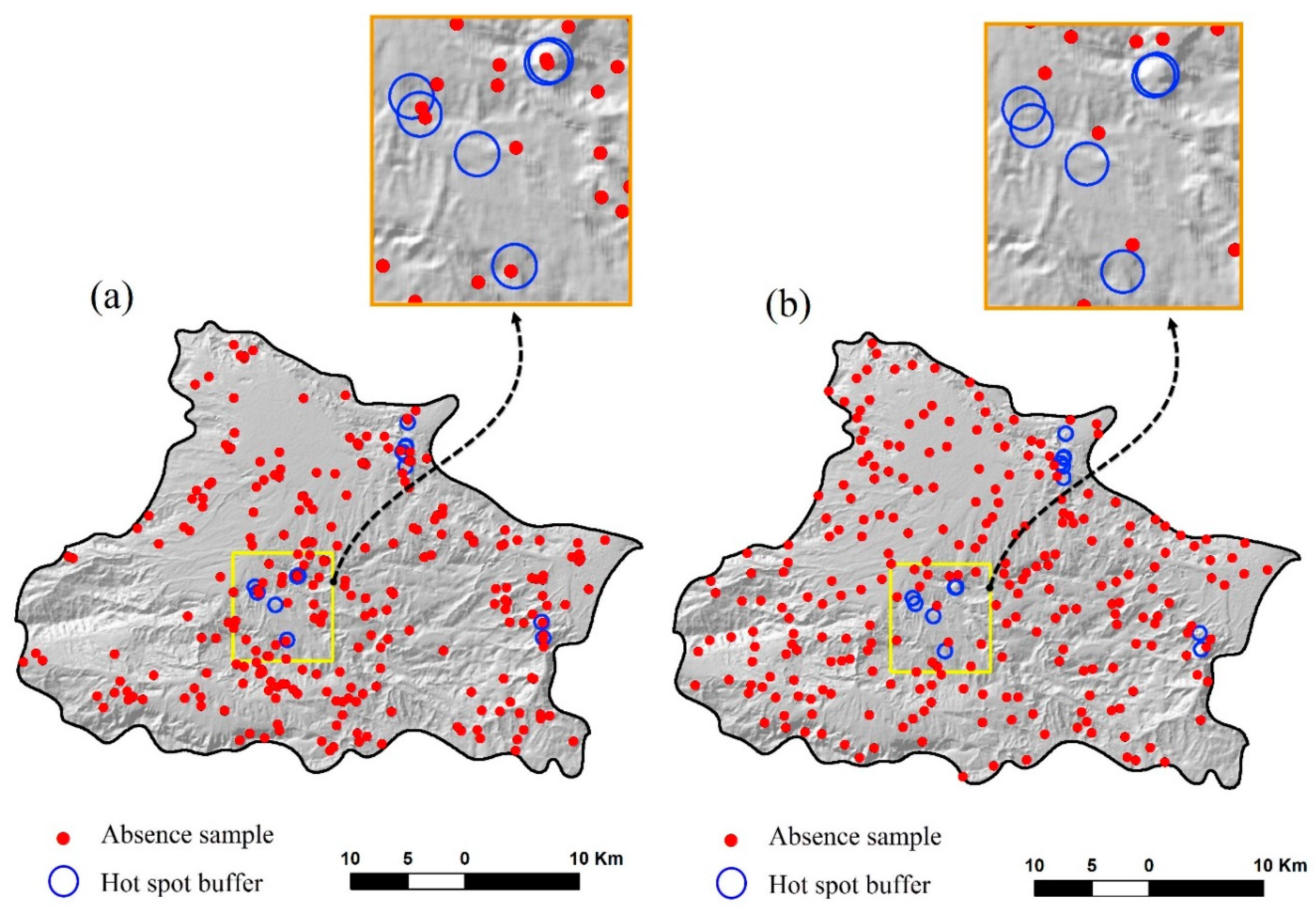
4.1. Selection of Absence Samples and Accuracy Assessment

The accuracies of the models in the training step (goodness-of-fit) are summarized in Table 5. When the RF model used the absence points produced by the SAS method, it had an AUC-ROC value of 0.944, whereas the AUC-ROC value was lower (0.926) in the simple random sampling method. Threshold-dependent evaluation metrics shed more light on the learning capability of the RF model in both sampling strategies and clearly confirmed the higher accuracy of the RF model in the SAS method (TSS = 0.891, E = 0.946, TPR = 0.938, FPR = 0.046, TNR = 0.953, FNR = 0.061) than in the simple random sampling method (TSS = 0.852, E = 0.926, TPR = 0.921, FPR = 0.069, TNR = 0.0931, FNR = 0.061).
For the MARS model, the SAS method also gave a higher AUC-ROC value (0.925) in comparison with the simple random method (0.898). In addition, for the simple random method, the accuracy of the MARS model decreased in comparison with the SAS method based on threshold-dependent criteria (Table 5). The TSS, E, TPR, FPR, TNR, and FNR values in the SAS method were 0.852, 0.926, 0.921, 0.069, 0.931, and 0.078, respectively, while in the simple random method the corresponding values were 0.789, 0.894, 0.892, 0.102, 0.897, and 0.107, respectively. Therefore, there was better agreement between the predictions of both models and reality in the SAS method. However, while goodness-of-fit shows how well the model fits to the training dataset and also reflects the learning capability of the model, the prediction performance of the model cannot be judged by goodness-of-fit because it is measured by the training dataset already used for model calibration [31].
The predictive performances of the RF and MARS models with the different absence sample selection strategies are shown in Table 6. Both the RF (AUC-ROC = 0.913, TSS = 0.72) and MARS (AUC-ROC = 0.889 and TSS = 0.705) models showed better performance when absence samples generated by the SAS tool were used in modeling. When absence samples of the random method were used, the performances of both models were considerably lower, with the RF model showing an AUC-ROC of 0.872 and a TSS of 0.681, and the MARS model an AUC-ROC of 0.833 and a TSS of 0.67.
When the simple random method was used to generate absence samples, the RF model gave E = 0.906, TPR = 0.896, FPR = 0.082, TNR = 0.917, and FNR = 0.103, while MARS gave E = 0.86, TPR = 0.855, FPR = 0.135, TNR = 0.864, and FNR = 0.144. However, when using the SAS method, the RF (E = 0.926, TPR = 0.921, FPR = 0.067, TNR = 0.932, and FNR = 0.078) and MARS (E = 0.9, TPR = 0.905, FPR = 0.105, TNR = 0.894, and FNR = 0.094) models showed better predictive performance. Another important finding in this study was that the RF model outperformed the MARS model, irrespective of the absence sampling method used (Table 6).
In this study, both the RF and MARS models showed better performance when based on the newly developed SAS tool, because it overcomes all the disadvantages associated with the simple random method. The results obtained demonstrate that the method and strategy used for production of absence samples significantly influences model prediction accuracy. The most interesting finding was that absence samples created by the SAS tool had a dispersed distribution pattern and were far from hotspot areas. In addition, the average nearest neighbor method resulted in a more even distribution of selected samples, which were more representative of the overall situation in the study area. Since hotspot areas are statistically significant, the end visualization is less subjective. Through these advantages, the SAS tool can enhance the ability of models based on presence–absence samples. However, it is difficult to directly compare the results of this study with those in previous publications, because there is no standard method for producing absence samples in the field of groundwater potential mapping. In landslide susceptibility modeling, a previous study investigated the effects of absence samples on model prediction and suggested that a buffer around presence samples can efficiently increase the accuracy of absence samples [7]. In other environmental fields, sampling strategy has been shown to have a significant influence on model performance [78,79].
Despite this, the simple random method has been widely applied by researchers [24,35,44,80]. Another disadvantage of the simple random method is that each pixel of the study area, even presence locations, has an equal chance of being selected as an absence sample [51]. Moreover, the distribution pattern of the absence samples generated by the simple random method is sometimes clustered and consequently cannot be representative of the population (i.e., pixel values in the study area) [81,82]. When absence samples are not truly representative of the population, the resulting error in the model output is called a ‘sampling error’ [52,83]. Therefore, although the simple random method is easy to use, it does not consider any criteria or essential preconditions. These shortcomings prompted us to develop a new method for creating absence samples based on statistical and spatial analyses.

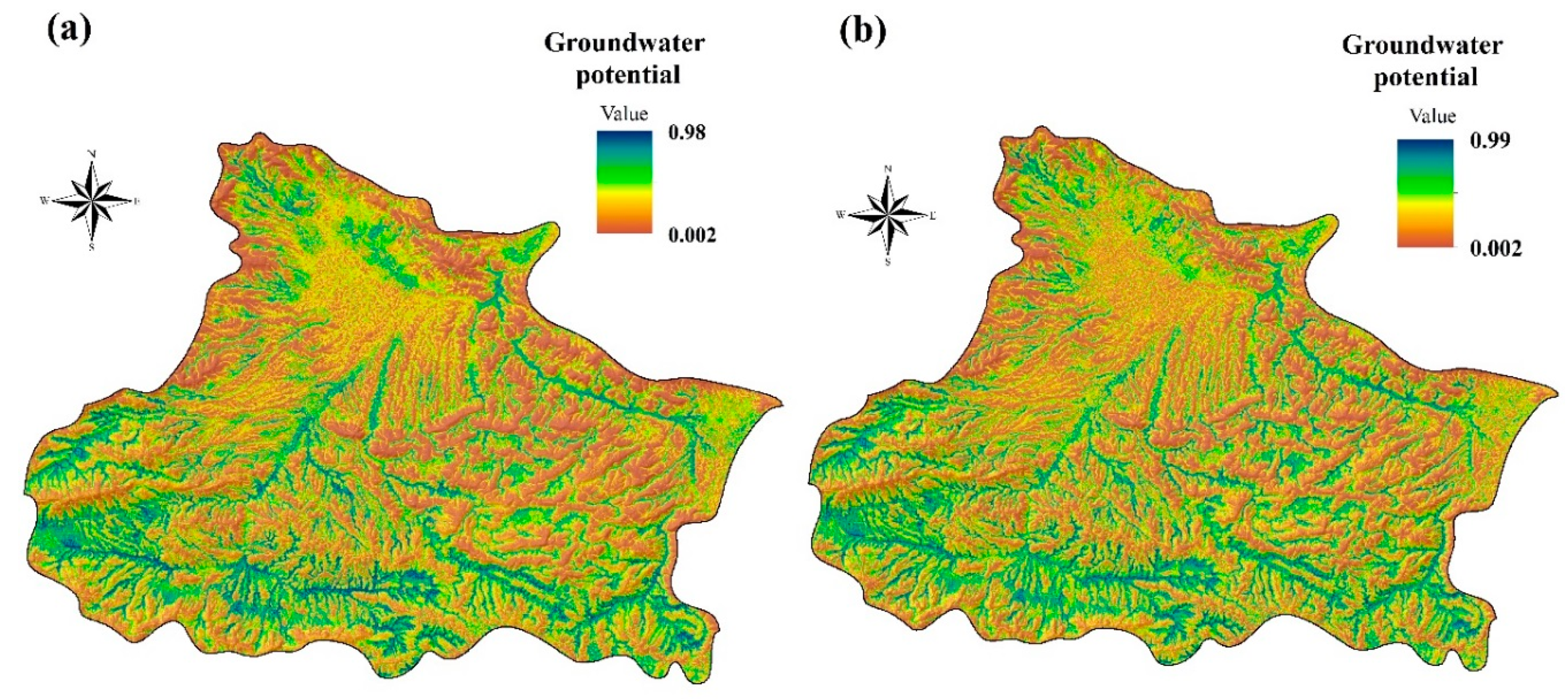
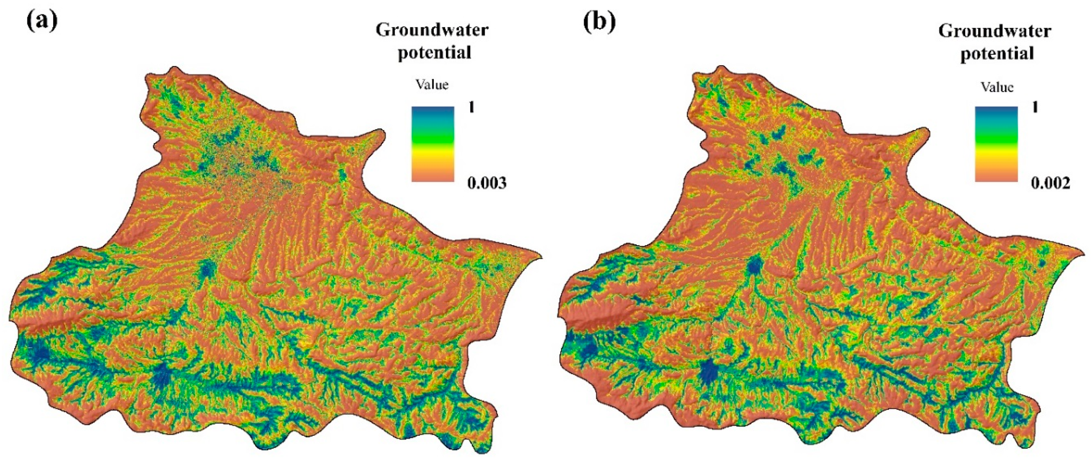
4.2. Groundwater Potential Mapping

The groundwater potential maps produced by the RF model based on the simple random method and the SAS method for producing absence samples are shown in Figure 9, while the corresponding maps created by the MARS model are shown in Figure 10. The blue color in the maps indicates high groundwater potential values, while red color indicates low values. All maps show high groundwater potential in southern parts of the study area. Table 7 shows the statistical characteristics of the probability values obtained from the RF and MARS models based on the simple random and SAS methods. As can be seen from the table, the RF method gave higher mean values and lower standard deviation with both the simple random and the SAS methods. From an aerial viewpoint, southern parts of the Bojnourd watershed have the highest groundwater potential based on both models. In this regard, others have reported a similar pattern for groundwater potential in this study area [43,73].
In this study, the RF and MARS methods were used to produce groundwater potential maps. Both models showed fairly good performance, but RF outperformed MARS based on the AUC-ROC and TSS evaluation criteria. RF is a powerful predictive model that combines several different decision trees to build a forest of trees [72]. In our earlier studies in the Mehran region, Iran, RF also demonstrated excellent performance in predicting groundwater potential [73]. Similar findings have been made in some other studies [10,15,82]. Appropriate determination of groundwater potential can help decision makers and stakeholders formulate effective groundwater policies and strategies [84,85].

5. Concluding Remarks

Sampling strategy is of great importance in groundwater potential modeling. However, selecting appropriate absence samples is a considerable challenge, and researchers often use a simple random sampling technique to deal with this challenge. The random sampling method can be a significant source of error in the groundwater modeling process. Hence, in this study, an automated, user-friendly tool for creating absence samples called selection of absence samples (SAS) was developed using the Python programming language. The SAS tool uses nearest neighbor index and hotspot analysis to produce robust and reliable absence samples. In a case study, the SAS tool was successfully applied to produce absence samples for groundwater potential modeling. The main finding of the study is that both the RF and MARS models showed better predictive performance when based on absence samples created by the SAS method rather than the simple random method. These findings improve understanding of the influence of sampling strategy on model output. Other data obtained in this study suggest that the SAS not only produces a proper distribution of absence samples, but also improves the performance of data mining and machine learning models for groundwater potential mapping. However, further research is needed to identify limitations of the SAS tool. In future investigations, it might be possible to consider topo-hydrological characteristics for selecting absence samples that enhance the efficiency of the SAS tool. Another task for future investigations is to investigate the performance of the SAS tool in a number of spatial modeling sub-fields (e.g., landslide, land subsidence, flooding).
Tool information
Name of tool: SAS (selection of absence samples)
Developers: Samadi, M., Rahmati, O.
Hardware required: General-purpose computer (3 Gb RAM)
Software required: ArcGIS 10.2 (or higher versions)
Program language: Python
Tool size: 5.1 kb
Cost: free of charge

Author Contributions

Conceptualization, O.R., D.D.M., and V.M.; Methodology, O.R., M.S., and S.L.; Software, O.R. and M.S.; Validation, O.R. and M.S.; Formal Analysis, O.R.; Data Curation, O.R. and D.D.M.; Writing—original draft preparation, O.R., Z.K., and D.T.B.; Writing—review & editing, Z.K., S.L., and D.T.B.; Visualization, O.R. and M.S.

Funding

This research received no external funding.

Acknowledgments

We greatly appreciate the assistance of the editor and anonymous reviewers for their constructive comments that helped us to improve the paper. We gratefully acknowledge the Iranian Department of Water Resources Management (IDWRM) and Department of Geological Survey of Iran (GSI) for providing necessary data and maps. This research was supported by the Basic Research Project of the Korea Institute of Geoscience and Mineral Resources (KIGAM) funded by the Ministry of Science and ICT and the Geographic Information Science Research Group, Ton Duc Thang University, Ho Chi Minh City, Viet Nam.

Conflicts of Interest

The authors declare no conflict of interest.

References

  1. Hong, H.; Pradhan, B.; Sameen, M.I.; Kalantar, B.; Zhu, A.; Chen, W. Improving the accuracy of landslide susceptibility model using a novel region-partitioning approach. Landslides 2018, 15, 753–772. [Google Scholar] [CrossRef]
  2. Van Westen, C.J.; Castellanos, E.; Kuriakose, S.L. Spatial data for landslide susceptibility, hazard, and vulnerability assessment: An overview. Eng. Geol. 2008, 102, 112–131. [Google Scholar] [CrossRef]
  3. Naghibi, S.A.; Pourghasemi, H.R. A comparative assessment between three machine learning models and their performance comparison by bivariate and multivariate statistical methods in groundwater potential mapping. Water Resour. Manag. 2015, 29, 5217–5236. [Google Scholar] [CrossRef]
  4. Nefeslioglu, H.A.; Gokceoglu, C.; Sonmez, H. An assessment on the use of logistic regression and artificial neural networks with different sampling strategies for the preparation of landslide susceptibility maps. Eng. Geol. 2008, 97, 171–191. [Google Scholar] [CrossRef]
  5. Corsini, A.; Cervi, F.; Ronchetti, F. Weight of evidence and artificial neural networks for potential groundwater spring mapping: An application to the Mt. Modino area (Northern Apennines, Italy). Geomorphology 2009, 111, 79–87. [Google Scholar] [CrossRef]
  6. Pradhan, B. A comparative study on the predictive ability of the decision tree, support vector machine and neuro-fuzzy models in landslide susceptibility mapping using GIS. Comput. Geosci. 2013, 51, 350–365. [Google Scholar] [CrossRef]
  7. Conoscenti, C.; Rotigliano, E.; Cama, M.; Caraballo-Arias, N.A.; Lombardo, L.; Agnesi, V. Exploring the effect of absence selection on landslide susceptibility models: A case study in Sicily, Italy. Geomorphology 2016, 261, 222–235. [Google Scholar] [CrossRef]
  8. Gorsevski, P.V.; Gessler, P.E.; Foltz, R.B.; Elliot, W.J. Spatial prediction of landslide hazard using logistic regression and ROC analysis. Trans. GIS 2006, 10, 395–415. [Google Scholar] [CrossRef]
  9. Formetta, G.; Capparelli, G.; Versace, P. Evaluating performance of simplified physically based models for shallow landslide susceptibility. Hydrol. Earth Syst. Sci. 2016, 20, 4585–4603. [Google Scholar] [CrossRef] [Green Version]
  10. Naghibi, S.A.; Pourghasemi, H.R.; Dixon, B. GIS-based groundwater potential mapping using boosted regression tree, classification and regression tree, and random forest machine learning models in Iran. Environ. Monit. Assess. 2016, 188, 44. [Google Scholar] [CrossRef]
  11. Wilson, J.P. Digital terrain modeling. Geomorphology 2012, 137, 107–121. [Google Scholar] [CrossRef]
  12. Tien Bui, D.; Pradhan, B.; Lofman, O.; Revhaug, I.; Dick, O.B. Landslide susceptibility mapping at Hoa Binh province (Vietnam) using an adaptive neuro-fuzzy inference system and GIS. Comput. Geosci. 2012, 45, 199–211. [Google Scholar] [CrossRef]
  13. Chen, T.-C.; Soo, V.-W. Feature Selection in Learning Common Sense Associations Using Matrix Factorization. Int. J. Fuzzy Syst. 2017, 19, 1217–1226. [Google Scholar] [CrossRef]
  14. Choubin, B.; Rahmati, O.; Soleimani, F.; Alilou, H.; Moradi, E.; Alamdari, N. Regional Groundwater Potential Analysis Using Classification and Regression Trees. In Spatial Modeling in GIS and R for Earth and Environmental Sciences; Elsevier: Amsterdam, The Netherlands, 2019; pp. 485–498. [Google Scholar]
  15. Golkarian, A.; Naghibi, S.A.; Kalantar, B.; Pradhan, B. Groundwater potential mapping using C5.0, random forest, and multivariate adaptive regression spline models in GIS. Environ. Monit. Assess. 2018, 190, 149. [Google Scholar] [CrossRef] [PubMed]
  16. Lee, S. Current and Future Status of GIS-based Landslide Susceptibility Mapping: A Literature Review. Korean J. Remote Sens. 2019, 35, 179–193. [Google Scholar]
  17. Ahlmer, A.-K.; Cavalli, M.; Hansson, K.; Koutsouris, A.J.; Crema, S.; Kalantari, Z. Soil moisture remote-sensing applications for identification of flood-prone areas along transport infrastructure. Environ. Earth Sci. 2018, 77, 533. [Google Scholar] [CrossRef] [Green Version]
  18. Falah, F.; Rahmati, O.; Rostami, M.; Ahmadisharaf, E.; Daliakopoulos, I.N.; Pourghasemi, H.R. Artificial Neural Networks for Flood Susceptibility Mapping in Data-Scarce Urban Areas. In Spatial Modeling in GIS and R for Earth and Environmental Sciences; Elsevier: Amsterdam, The Netherlands, 2019; pp. 323–336. [Google Scholar]
  19. Pham, B.T.; Prakash, I.; Singh, S.K.; Shirzadi, A.; Shahabi, H.; Bui, D.T. Landslide susceptibility modeling using Reduced Error Pruning Trees and different ensemble techniques: Hybrid machine learning approaches. Catena 2019, 175, 203–218. [Google Scholar] [CrossRef]
  20. Plug, C.; Xia, J.C.; Caulfield, C. Spatial and temporal visualisation techniques for crash analysis. Accid. Anal. Prev. 2011, 43, 1937–1946. [Google Scholar] [CrossRef] [PubMed]
  21. Pourghasemi, H.R.; Rahmati, O. Prediction of the landslide susceptibility: Which algorithm, which precision? Catena 2018, 162, 177–192. [Google Scholar] [CrossRef]
  22. Conoscenti, C.; Angileri, S.; Cappadonia, C.; Rotigliano, E.; Agnesi, V.; Märker, M. Gully erosion susceptibility assessment by means of GIS-based logistic regression: A case of Sicily (Italy). Geomorphology 2014, 204, 399–411. [Google Scholar] [CrossRef] [Green Version]
  23. Gayen, A.; Pourghasemi, H.R.; Saha, S.; Keesstra, S.; Bai, S. Gully erosion susceptibility assessment and management of hazard-prone areas in India using different machine learning algorithms. Sci. Total Environ. 2019, 668, 124–138. [Google Scholar] [CrossRef] [PubMed]
  24. Pourghasemi, H.R.; Yousefi, S.; Kornejady, A.; Cerdà, A. Performance assessment of individual and ensemble data-mining techniques for gully erosion modeling. Sci. Total Environ. 2017, 609, 764–775. [Google Scholar] [CrossRef] [PubMed] [Green Version]
  25. Rahmati, O.; Tahmasebipour, N.; Haghizadeh, A.; Pourghasemi, H.R.; Feizizadeh, B. Evaluation of different machine learning models for predicting and mapping the susceptibility of gully erosion. Geomorphology 2017, 298, 118–137. [Google Scholar] [CrossRef]
  26. Lee, S.; Lee, C.-W. Application of decision-tree model to groundwater productivity-potential mapping. Sustainability 2015, 7, 13416–13432. [Google Scholar] [CrossRef]
  27. Lee, S.; Park, I.; Choi, J.-K. Spatial prediction of ground subsidence susceptibility using an artificial neural network. Environ. Manag. 2012, 49, 347–358. [Google Scholar] [CrossRef] [PubMed]
  28. Park, I.; Choi, J.; Lee, M.J.; Lee, S. Application of an adaptive neuro-fuzzy inference system to ground subsidence hazard mapping. Comput. Geosci. 2012, 48, 228–238. [Google Scholar] [CrossRef]
  29. Pourghasemi, H.R.; Saravi, M.M. Land-Subsidence Spatial Modeling Using the Random Forest Data-Mining Technique. In Spatial Modeling in GIS and R for Earth and Environmental Sciences; Elsevier: Amsterdam, The Netherlands, 2019; pp. 147–159. [Google Scholar]
  30. Rahmati, O.; Golkarian, A.; Biggs, T.; Keesstra, S.; Mohammadi, F.; Daliakopoulos, I.N. Land subsidence hazard modeling: Machine learning to identify predictors and the role of human activities. J. Environ. Manag. 2019, 236, 466–480. [Google Scholar] [CrossRef]
  31. Bui, D.T.; Tuan, T.A.; Klempe, H.; Pradhan, B.; Revhaug, I. Spatial prediction models for shallow landslide hazards: A comparative assessment of the efficacy of support vector machines, artificial neural networks, kernel logistic regression, and logistic model tree. Landslides 2016, 13, 361–378. [Google Scholar]
  32. Chapi, K.; Singh, V.P.; Shirzadi, A.; Shahabi, H.; Bui, D.T.; Pham, B.T.; Khosravi, K. A novel hybrid artificial intelligence approach for flood susceptibility assessment. Environ. Modell. Softw. 2017, 95, 229–245. [Google Scholar] [CrossRef]
  33. Kalantari, Z.; Ferreira, C.S.S.; Koutsouris, A.J.; Ahmer, A.-K.; Cerdà, A.; Destouni, G. Assessing flood probability for transportation infrastructure based on catchment characteristics, sediment connectivity and remotely sensed soil moisture. Sci. Total Environ. 2019, 661, 393–406. [Google Scholar] [CrossRef]
  34. Rutherford, G.; Guisan, A.; Zimmermann, N. Evaluating sampling strategies and logistic regression methods for modelling complex land cover changes. J. Appl. Ecol. 2007, 44, 414–424. [Google Scholar] [CrossRef]
  35. Tehrany, M.S.; Pradhan, B.; Jebur, M.N. Flood susceptibility mapping using a novel ensemble weights-of-evidence and support vector machine models in GIS. J. Hydrol. 2014, 512, 332–343. [Google Scholar] [CrossRef]
  36. Tehrany, M.S.; Pradhan, B.; Mansor, S.; Ahmad, N. Flood susceptibility assessment using GIS-based support vector machine model with different kernel types. Catena 2015, 125, 91–101. [Google Scholar] [CrossRef]
  37. Termeh, S.V.R.; Kornejady, A.; Pourghasemi, H.R.; Keesstra, S. Flood susceptibility mapping using novel ensembles of adaptive neuro fuzzy inference system and metaheuristic algorithms. Sci. Total Environ. 2018, 615, 438–451. [Google Scholar] [CrossRef] [PubMed]
  38. Perry, G.L.; Dickson, M.E. Using Machine Learning to Predict Geomorphic Disturbance: The Effects of Sample Size, Sample Prevalence, and Sampling Strategy. J. Geophys. Res.-Earth 2018, 123, 2954–2970. [Google Scholar] [CrossRef]
  39. Xu, C.; He, H.S.; Hu, Y.; Chang, Y.; Li, X.; Bu, R. Latin hypercube sampling and geostatistical modeling of spatial uncertainty in a spatially explicit forest landscape model simulation. Ecol. Model. 2005, 185, 255–269. [Google Scholar] [CrossRef]
  40. Sameen, M.I.; Pradhan, B.; Lee, S. Self-learning random forests model for mapping groundwater yield in data-scarce areas. Nat. Resour. Res. 2018, 28, 757–775. [Google Scholar] [CrossRef]
  41. Zabihi, M.; Pourghasemi, H.R.; Pourtaghi, Z.S.; Behzadfar, M. GIS-based multivariate adaptive regression spline and random forest models for groundwater potential mapping in Iran. Environ. Earth Sci. 2016, 75, 665. [Google Scholar] [CrossRef]
  42. Ichnowski, J.; Alterovitz, R. Fast nearest neighbor search in SE (3) for sampling-based motion planning. In Algorithmic Foundations of Robotics XI; Springer: Berlin/Heidelberg, Germany, 2015; pp. 197–214. [Google Scholar]
  43. Vadrevu, K.P.; Badarinath, K.; Anuradha, E. Spatial patterns in vegetation fires in the Indian region. Environ. Monit. Assess. 2008, 147, 1. [Google Scholar] [CrossRef] [PubMed]
  44. Chen, W.; Li, H.; Hou, E.; Wang, S.; Wang, G.; Panahi, M.; Li, T.; Peng, T.; Guo, C.; Niu, C. GIS-based groundwater potential analysis using novel ensemble weights-of-evidence with logistic regression and functional tree models. Sci. Total Environ. 2018, 634, 853–867. [Google Scholar] [CrossRef] [Green Version]
  45. Chen, Y.; Ge, Y. Spatial point pattern analysis on the villages in China’s poverty-stricken areas. Procedia Environ. Sci. 2015, 27, 98–105. [Google Scholar] [CrossRef]
  46. Bajat, B.; Blagojević, D.; Kilibarda, M.; Luković, J.; Tošić, I. Spatial analysis of the temperature trends in Serbia during the period 1961–2010. Theor. Appl. Climatol. 2015, 121, 289–301. [Google Scholar] [CrossRef]
  47. Koch, S.L.; Shriver, M.D.; Jablonski, N.G. Variation in human hair ultrastructure among three biogeographic populations. J. Struct. Biol. 2019, 205, 60–66. [Google Scholar] [CrossRef] [PubMed]
  48. Prasannakumar, V.; Vijith, H.; Charutha, R.; Geetha, N. Spatio-temporal clustering of road accidents: GIS based analysis and assessment. Proc. Soc. Behv. 2011, 21, 317–325. [Google Scholar] [CrossRef]
  49. Zou, G.; Wu, H.-I. Nearest-neighbor distribution of interacting biological entities. J. Theor. Biol. 1995, 172, 347–353. [Google Scholar] [CrossRef] [PubMed]
  50. Bishop, M.A. Nearest neighbor analysis of mega-barchanoid dunes, Ar Rub’al Khali, sand sea: The application of geographical indices to the understanding of dune field self-organization, maturity and environmental change. Geomorphology 2010, 120, 186–194. [Google Scholar] [CrossRef]
  51. Chainey, S. Advanced Hotspot Analysis: Spatial Significance Mapping Using Gi*; UCL Jill Dando Institute of Crime Science, University College London: London, UK, 2010. [Google Scholar]
  52. McMillan, H.; Jackson, B.; Clark, M.; Kavetski, D.; Woods, R. Rainfall uncertainty in hydrological modelling: An evaluation of multiplicative error models. J. Hydrol. 2011, 400, 83–94. [Google Scholar] [CrossRef]
  53. Pal, M. Random forest classifier for remote sensing classification. Int. J. Remote Sens. 2005, 26, 217–222. [Google Scholar] [CrossRef]
  54. Kiss, R. Determination of drainage network in digital elevation models, utilities and limitations. J. Hung. Geomath. 2004, 2, 16–29. [Google Scholar]
  55. San, B.T. An evaluation of SVM using polygon-based random sampling in landslide susceptibility mapping: The Candir catchment area (western Antalya, Turkey). Int. J. Appl. Earth Obs. Geoinf. 2014, 26, 399–412. [Google Scholar] [CrossRef]
  56. Beven, K.J.; Kirkby, M.J. A physically based, variable contributing area model of basin hydrology/Un modèle à base physique de zone d’appel variable de l’hydrologie du bassin versant. Hydrol. Sci. J. 1979, 24, 43–69. [Google Scholar] [CrossRef]
  57. Breiman, L. Random forests. Mach. Learn. 2001, 45, 5–32. [Google Scholar] [CrossRef]
  58. Wang, Z.; Lai, C.; Chen, X.; Yang, B.; Zhao, S.; Bai, X. Flood hazard risk assessment model based on random forest. J. Hydrol. 2015, 527, 1130–1141. [Google Scholar] [CrossRef]
  59. Qi, Y. Random forest for bioinformatics. In Ensemble Machine Learning; Springer: Berlin/Heidelberg, Germany, 2012; pp. 307–323. [Google Scholar]
  60. Archer, K.J.; Kimes, R.V. Empirical characterization of random forest variable importance measures. Comput. Stat. Data Anal. 2008, 52, 2249–2260. [Google Scholar] [CrossRef]
  61. Devetyarov, D.; Nouretdinov, I. Prediction with confidence based on a random forest classifier. In Proceedings of the IFIP International Conference on Artificial Intelligence Applications and Innovations, Larnaca, Cyprus, 6–7 October 2010; pp. 37–44. [Google Scholar]
  62. Friedman, J.H. Multivariate adaptive regression splines. Ann. Stat. 1991, 19, 1–67. [Google Scholar] [CrossRef]
  63. Gutiérrez, Á.G.; Schnabel, S.; Contador, J.F.L. Using and comparing two nonparametric methods (CART and MARS) to model the potential distribution of gullies. Ecol. Model. 2009, 220, 3630–3637. [Google Scholar] [CrossRef]
  64. Leathwick, J.; Elith, J.; Hastie, T. Comparative performance of generalized additive models and multivariate adaptive regression splines for statistical modelling of species distributions. Ecol. Model. 2006, 199, 188–196. [Google Scholar] [CrossRef]
  65. Leathwick, J.; Rowe, D.; Richardson, J.; Elith, J.; Hastie, T. Using multivariate adaptive regression splines to predict the distributions of New Zealand’s freshwater diadromous fish. Freshw. Biol. 2005, 50, 2034–2052. [Google Scholar] [CrossRef]
  66. Lee, T.S.; Chiu, C.-C.; Chou, Y.-C.; Lu, C.-J. Mining the customer credit using classification and regression tree and multivariate adaptive regression splines. Comput. Stat. Data Anal. 2006, 50, 1113–1130. [Google Scholar] [CrossRef]
  67. Lacoste, M.; Lemercier, B.; Walter, C. Regional mapping of soil parent material by machine learning based on point data. Geomorphology 2011, 133, 90–99. [Google Scholar] [CrossRef]
  68. Lee, S.; Hong, S.M.; Jung, H.S. GIS-based groundwater potential mapping using artificial neural network and support vector machine models: The case of Boryeong city in Korea. Geocarto Int. 2018, 33, 847–861. [Google Scholar] [CrossRef]
  69. Lee, S.; Park, I. Application of decision tree model for the ground subsidence hazard mapping near abandoned underground coal mines. J. Environ. Manag. 2013, 127, 166–176. [Google Scholar] [CrossRef] [PubMed]
  70. Allouche, O.; Tsoar, A.; Kadmon, R. Assessing the accuracy of species distribution models: Prevalence, kappa and the true skill statistic (TSS). J. Appl. Ecol. 2006, 43, 1223–1232. [Google Scholar] [CrossRef]
  71. Peres, D.; Cancelliere, A. Derivation and evaluation of landslide-triggering thresholds by a Monte Carlo approach. Hydrol. Earth Syst. Sci. 2014, 18, 4913–4931. [Google Scholar] [CrossRef] [Green Version]
  72. Pradhan, B.; Lee, S.; Buchroithner, M.F. A GIS-based back-propagation neural network model and its cross-application and validation for landslide susceptibility analyses. Comput. Environ. Urban 2010, 34, 216–235. [Google Scholar] [CrossRef]
  73. Rahmati, O.; Naghibi, S.A.; Shahabi, H.; Bui, D.T.; Pradhan, B.; Azareh, A.; Rafiei-Sardooi, E.; Samani, A.N.; Melesse, A.M. Groundwater spring potential modelling: Comprising the capability and robustness of three different modeling approaches. J. Hydrol. 2018, 565, 248–261. [Google Scholar] [CrossRef]
  74. Frattini, P.; Crosta, G.; Carrara, A. Techniques for evaluating the performance of landslide susceptibility models. Eng. Geol. 2010, 111, 62–72. [Google Scholar] [CrossRef]
  75. Greiner, M.; Pfeiffer, D.; Smith, R. Principles and practical application of the receiver-operating characteristic analysis for diagnostic tests. Prev. Vet. Med. 2000, 45, 23–41. [Google Scholar] [CrossRef]
  76. Hussin, H.Y.; Zumpano, V.; Reichenbach, P.; Sterlacchini, S.; Micu, M.; van Westen, C.; Bălteanu, D. Different landslide sampling strategies in a grid-based bi-variate statistical susceptibility model. Geomorphology 2016, 253, 508–523. [Google Scholar] [CrossRef]
  77. Rahmati, O.; Kornejady, A.; Samadi, M.; Deo, R.C.; Conoscenti, C.; Lombardo, L.; Dayal, K.; Taghizadeh-Mehrjardi, R.; Pourghasemi, H.R.; Kumar, S. PMT: New analytical framework for automated evaluation of geo-environmental modelling approaches. Sci. Total Environ. 2019, 664, 296–311. [Google Scholar] [CrossRef] [PubMed]
  78. Wang, L.-J.; Sawada, K.; Moriguchi, S. Landslide susceptibility analysis with logistic regression model based on FCM sampling strategy. Comput. Geosci. 2013, 57, 81–92. [Google Scholar] [CrossRef]
  79. Zhou, L. Performance of corporate bankruptcy prediction models on imbalanced dataset: The effect of sampling methods. Knowl.-Based Syst. 2013, 41, 16–25. [Google Scholar] [CrossRef]
  80. Kordestani, M.D.; Naghibi, S.A.; Hashemi, H.; Ahmadi, K.; Kalantar, B.; Pradhan, B. Groundwater potential mapping using a novel data-mining ensemble model. Hydrogeol. J. 2019, 27, 211–224. [Google Scholar] [CrossRef]
  81. Sharma, G. Pros and cons of different sampling techniques. Int. J. Appl. Res. 2017, 3, 749–752. [Google Scholar]
  82. Ye, Y.; Wu, Q.; Huang, J.Z.; Ng, M.K.; Li, X. Stratified sampling for feature subspace selection in random forests for high dimensional data. Pattern Recogn. 2013, 46, 769–787. [Google Scholar] [CrossRef]
  83. Cardini, A.; Elton, S. Sample size and sampling error in geometric morphometric studies of size and shape. Zoomorphology 2007, 126, 121–134. [Google Scholar] [CrossRef]
  84. Jha, M.K.; Chowdary, V.; Chowdhury, A. Groundwater assessment in Salboni Block, West Bengal (India) using remote sensing, geographical information system and multi-criteria decision analysis techniques. Hydrogeol. J. 2010, 18, 1713–1728. [Google Scholar] [CrossRef]
  85. Saha, D.; Ray, R.K. Groundwater resources of India: Potential, challenges and management. In Groundwater Development and Management; Springer: Berlin/Heidelberg, Germany, 2019; pp. 19–42. [Google Scholar]
Figure 1. A conceptual architecture (processing steps) for generating absence samples by the Selection of Absence Samples (SAS) tool.
Remotesensing 11 01375 g001
Figure 2. Schematic diagram of the relationship between the distribution pattern of samples and the nearest neighbor (NN) index.
Remotesensing 11 01375 g002
Figure 3. Schematic diagram of hotspot determination using Gi* metric.
Remotesensing 11 01375 g003
Figure 4. A view of the Selection of Absence Samples (SAS) tool and its components.
Remotesensing 11 01375 g004
Figure 5. Map showing location of the study area in northern Iran and location of springs within the area.
Remotesensing 11 01375 g005
Figure 6. Maps of absence samples produced using (a) a random sampling method, and (b) the selection of absence samples (SAS) method.
Remotesensing 11 01375 g006
Figure 7. Groundwater-affecting factors (GAFs) in the study area: (a) altitude, (b) slope, (c) aspect, (d) convergence index, (e) distance from fault, and (f) distance from stream (for a detailed description of lithological classes, see Table 3).
Remotesensing 11 01375 g007
Figure 8. Groundwater-affecting factors in the study area: (a) stream density, (b) relative slope position, (c) topographic position index, (d) terrain ruggedness index, (e) topographic wetness index, and (f) lithology (for a detailed description of lithological classes, see Table 3).
Remotesensing 11 01375 g008
Figure 9. Groundwater potential maps of the study area produced using the random forest (RF) model and based on: (a) the simple random method, and (b) the selection of absence samples (SAS) method.
Remotesensing 11 01375 g009
Figure 10. Groundwater potential maps of the study area produced using the multivariate adaptive regression splines (MARS) model and based on: (a) the simple random method, and (b) the selection of absence samples (SAS) method.
Remotesensing 11 01375 g010
Table 1. Input parameters and files for the Selection of Absence Samples (SAS) tool.
IDSettingDescription
1Input a layer of presence samplesThe layer of presence samples (positive points) showing the location of occurrences for a given phenomenon should be input in this field. For example, a spring file (include locations and groundwater discharge) should be introduced here.
2Weight of presence samplesEach presence sample has a value or weight. For example, springs have groundwater discharge.
3Radius of circles (Buffer for presence samples)Buffer for presence samples should be determined. These buffer/circles do not allow random absence samples to be placed inside them. Therefore, absence samples are placed in an area that is free of the given phenomenon (e.g., landslide-free area, spring-free area).
4Hotspot circles (buffer for hotspots)After determining hotspot locations, users should determine a buffer for them that does not allow absence samples to be placed there.
5Number of absence samplesIn general, the number of absence samples is equal to the number of presence samples. The number of absence samples usually influences the model output.
6Boundary of the study areaThe SAS tool needs a specific area such as a study area to determine the permitted sites for producing absence samples. Users can introduce the study area file for this field.
Table 2. Output files of the Selection of Absence Samples (SAS) tool.
IDSettingDescription
1Absence samples layerThis file is the main output of the SAS tool, and explains the location of absence samples in the study area. These absence samples are produced based on average nearest neighbor and hotspot analyses. This approach for producing absence samples is better than the simple random method.
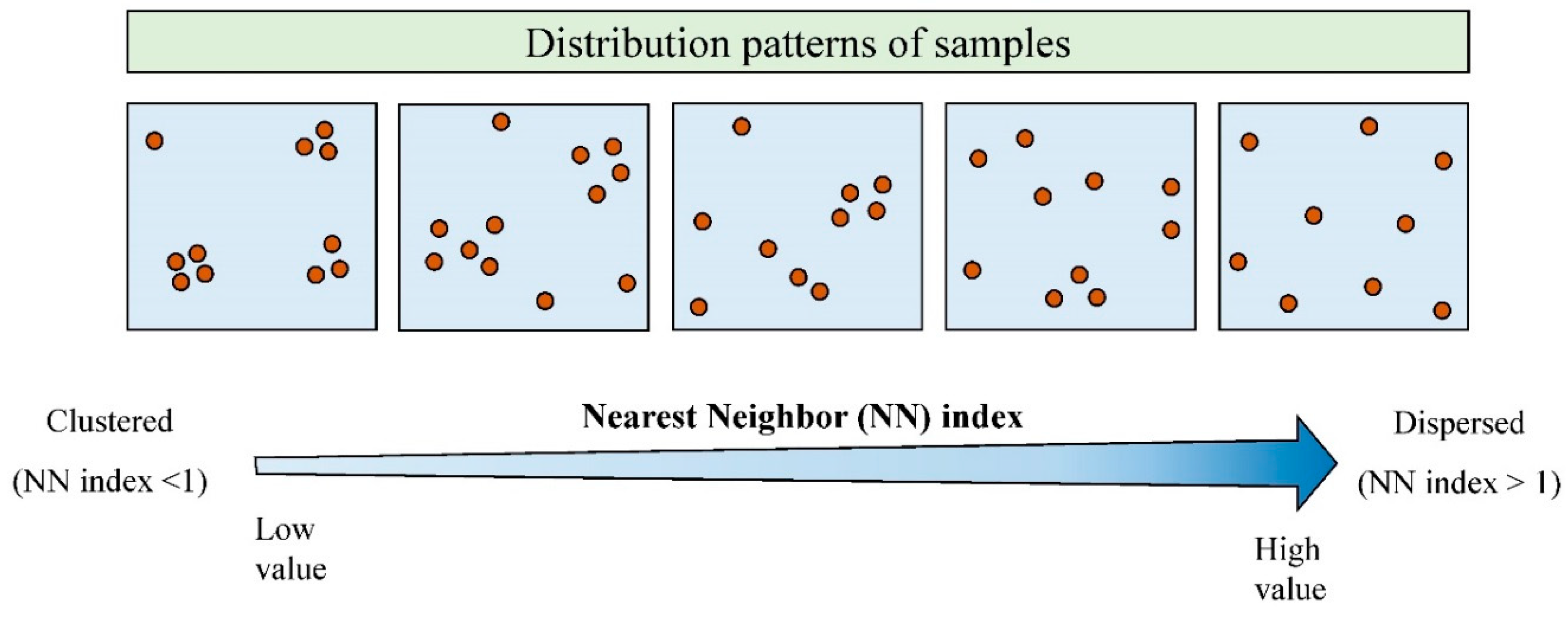
2Hotspot and coldspot layerThis file shows the result of hotspot analysis. It classifies presence samples into three groups: coldspot, medium, and hotspot. This type of classification is based on the value of presence samples (e.g., groundwater discharge) and their distance from each other.
3Significant hotspot samplesThis layer explains which presence samples are significant hotspots in comparison with other presence samples. The selection of hotspot samples depends on both z-score and p-value in hotspot analysis based on the Gi* metric.
Table 3. Lithology of the study area.
EraPeriodLithology
CenozoicQuaternary (Q)Low level piedmont fan and valley terrace deposits
CenozoicNeogene (N)Red marl, gypsiferous marl, sandstone, and conglomerate
MesozoicCretaceous (C) Olive green glauconitic sandstone and shale
MesozoicEarly Cretaceous (EC)Ammonite bearing shale with orbitolin limestone
MesozoicJurassic-Cretaceous (JC) Pale red argillaceous limestone, sandstone, and conglomerate
MesozoicTriassic–Jurassic (TJ)Subordinate sandy limestone, dark grey shale, and sandstone
Table 4. Contingency matrix used for evaluation of models.
ObservedPredicted
Non-OccurrenceOccurrence
Non-occurrenceTrue negative (TN)False positive (FP)
OccurrenceFalse negative (FN)True positive (TP)
Table 5. Goodness-of-fit of the random forest (RF) and multivariate adaptive regression splines (MARS) models in different sampling strategies.
Sampling StrategiesEvaluation CriteriaModels
RFMARS
Selection of Absence Samples (SAS) methodAUC-ROC 10.9440.925
TSS 20.8910.852
Efficiency (E)0.9460.926
True positive rate (TPR)0.9380.921
False positive rate (FPR)0.0460.069
True negative rate (TNR)0.9530.931
False negative rate (FNR)0.0610.078
Simple random methodAUC-ROC 10.9260.898
TSS 20.8520.789
Efficiency (E)0.9260.894
True positive rate (TPR)0.9210.892
False positive rate (FPR)0.0690.102
True negative rate (TNR)0.9310.897
False negative rate (FNR)0.0780.107
1 Area under the receiver operating characteristic curve; 2 True skill statistic.
Table 6. Predictive performance of the random forest (RF) and multivariate adaptive regression splines (MARS) models in different sampling strategies.
Sampling StrategyEvaluation CriteriaModels
RFMARS
Selection of Absence Samples (SAS) methodAUC-ROC 10.9130.889
TSS 20.720.705
Efficiency (E)0.9260.90
True positive rate (TPR)0.9210.905
False positive rate (FPR)0.0670.105
True negative rate (TNR)0.9320.894
False negative rate (FNR)0.0780.094
Simple random methodAUC-ROC 10.8720.833
TSS 20.6810.67
Efficiency (E)0.9060.86
True positive rate (TPR)0.8960.855
False positive rate (FPR)0.0820.135
True negative rate (TNR)0.9170.864
False negative rate (FNR)0.1030.144
1 Area under the receiver operating characteristic curve; 2 True skill statistic.
Table 7. Statistical characteristics of the probability values obtained from the random forest (RF) and multivariate adaptive regression splines (MARS) models based on the simple random and selection of absence samples (SAS) methods.
ModelSimple Random MethodSAS Method
MinimumMaximumMeanSDMinimumMaximumMeanSD
RF0.0020.9890.3390.2280.0030.9940.3510.232
MARS0.0101.0000.3090.3070.0101.0000.2870.300
SD: Standard Deviation.

