Refined Model-Based and Feature-Driven Extraction of Buildings from PolSAR Images

Abstract

Polarimetric synthetic aperture radar (PolSAR) building extraction plays an important role in urban planning, disaster management, etc. In this paper, a building extraction method using refined model-based decomposition and robust scattering feature is proposed. On the one hand, the newly proposed refined five-component decomposition and its derived scattering powers are applied to detect the buildings. On the other hand, by combining the matrix elements and co-polarization correlation coefficient, a robust feature is proposed to discriminate buildings and non-buildings. Both these two preliminary extraction results are obtained through thresholding segmentation. Finally, they are fused via the HX Markov random fields so as to further improve the extraction accuracy. The performance of the proposed method is demonstrated and evaluated with Gaofen-3 and uninhabited aerial vehicle SAR full PolSAR data over different test sites. Outputs show that the proposed method outperforms other state-of-the-art methods and provides an overall accuracy of over 90%.

1. Introduction

Building extraction has attracted continuous attention since it plays an important role in damage assessment, population estimation, city expansion, and other remote sensing applications in the military and civilian fields [1,2,3,4,5,6,7,8,9,10,11,12,13,14]. Polarimetric synthetic aperture radar (PolSAR) is an active, high-resolution and multimode operating radar system, which provides abundant information for quick remote sensing in almost all weather and solar illumination conditions. PolSAR data provide a possibility to separate scattering contributions of different terrains, which can be associated with certain elementary scattering characteristics [15,16,17,18,19,20,21]. This scattering characteristics-based PolSAR data processing enables interpretation of radar images more easily and thus, is of great importance in building extraction.

In recent decades, there were numerous studies which investigated this field. For instance, Xiang et al. [2] incorporated the cross-scattering model and polarimetric coherence into the fusion of correlated probabilities to extract built-up areas. Quan et al. [3] constructed two extractors by using the eigenvalues to delineate buildings with different orientations. Azmedroub et al. [4] applied the Yamaguchi four-component decomposition and circular polarimetric covariance matrix to detect buildings. Susaki et al. [5] utilized the volume scattering power, the total power, and co-polarization coherence to discriminate buildings. On this basis, Kajimoto et al. [6] replaced the co-polarization coherence with the POA randomness to further discriminate buildings. These methods introduced various features on the basis of model-based decomposition (MBD) and have met with different degrees of success. Despite all this, there still exist certain drawbacks for these methods. On the one hand, the scattering model involved in the MBD is inappropriate for building scattering interpretation because of the severe overestimation of volume scattering (OVS) [22,23]. On the other hand, the incorporated features are generally data-dependent such that the extraction results are non-robust when applied for different data.

To address these problems, this paper proposes a building extraction method with refined model-based decomposition and robust scattering feature for PolSAR images. First, the scattering powers derived from the refined five component decomposition (R5CD) [24] are integrated. The R5CD is our newly proposed work, which can characterize building scattering by significantly improving the OVS. Second, concerning the variety of scattering characteristics, a robust feature combing the matrix elements and the co-polarization correlation coefficient is proposed. Through setting different thresholds, buildings and non-buildings can be separately highlighted using the above methodologies. Finally, these two preliminary results are fused through the HX Markov random fields (HX–MRF) image fusion algorithm [25] to further improve the extraction accuracy. The performance of the proposed method is demonstrated and evaluated with Gaofen-3 (GF-3) and uninhabited aerial vehicle SAR (UAVSAR) full PolSAR data over different test sites. Outputs show that the proposed method provides an overall accuracy of over 90%, which outperforms other state-of-the-art methods.

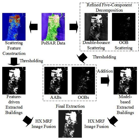
2. Methodology

2.1. Refined Model-based Building Extraction

The scattering power from buildings primarily includes co-polarization power induced by buildings approximately aligned with the flight trajectory (AABs) and cross-polarization power induced by buildings with oblique orientations (OOBs) [22,23]. For AABs, it is well recognized that the double-bounce scattering power can be directly used for extraction. Whereas for OOBs, a more sophisticated scattering model needs to be considered because the general double-bounce scattering does not support their dominant mechanism and the traditional MBDs generally cause severe OVS. Recently, an OOB scattering model along with an R5CD scheme was proposed, which can effectively characterize building scattering by reducing the volume scattering and enhancing the OOB scattering simultaneously. Considering this, this section briefly reviews the R5CD [24] and presents an R5CD-based building extraction method which detects the AABs and OOBs, respectively.

Subject to the reciprocity condition, the acquired coherency matrix can be presented as:

$$\langle [\mathit{T}]\rangle =\langle {\mathit{k}}_{3\mathrm{p}}{\mathit{k}}_{3\mathrm{p}}^{\mathrm{H}}\rangle =\left[\begin{array}{ccc}{T}_{11}& T_{12}& T_{13}\\ T_{21}& T_{22}& T_{23}\\ T_{31}& T_{32}& T_{33}\end{array}\right]$$

(1)

where $k_{3p}$ represents the Pauli vector. The superscript H and the notation 〈 〉 indicate the conjugate transpose and ensemble averaging, respectively. In the R5CD, the coherency matrix is decomposed as a weighted sum of five kinds of basic scattering, i.e., surface, double-bounce, helix, volume, and OOB scattering, which is given as

$$\langle [\mathit{T}]\rangle =f_{\mathrm{S}}{[\mathit{T}]}_{\mathrm{S}}+f_{\mathrm{D}}{[\mathit{T}]}_{\mathrm{D}}+f_{\mathrm{H}}{[\mathit{T}]}_{\mathrm{H}}+f_{\mathrm{V}}{[\mathit{T}]}_{\mathrm{V}}+f_{\mathrm{O}}{[\mathit{T}]}_{\mathrm{O}}$$

(2)

where $f_{\mathrm{S}}$, $f_{\mathrm{D}}$, $f_{\mathrm{H}}$, $f_{\mathrm{V}}$ and $f_{\mathrm{L}}$ are scattering coefficients to be computed. ${[\mathit{T}]}_{\mathrm{S}}$, ${[\mathit{T}]}_{\mathrm{D}}$, ${[\mathit{T}]}_{\mathrm{H}}$ and ${[\mathit{T}]}_{\mathrm{V}}$ are the models of surface, double-bounce, helix, and volume scatterings in the Yamaguchi four-component decomposition [26,27], respectively. Their mathematical forms are given as

$$\begin{array}{l}{[\mathit{T}]}_{\mathrm{S}}=\left[\begin{array}{ccc}1& {\beta }^{\ast }& 0\\ \beta & |\beta {|}^2& 0\\ 0& 0& 0\end{array}\right],{[\mathit{T}]}_{\mathrm{D}}=\left[\begin{array}{ccc}|\alpha {|}^2& \alpha & 0\\ {\alpha }^{\ast }& 1& 0\\ 0& 0& 0\end{array}\right]\\ {[\mathit{T}]}_{\mathrm{H}}=\frac{1}{2}\left[\begin{array}{ccc}0& 0& 0\\ 0& 1& \pm j\\ 0& \mp j& 1\end{array}\right],{[\mathit{T}]}_{\mathrm{V}}=\frac{1}{4}\left[\begin{array}{ccc}2& 0& 0\\ 0& 1& 0\\ 0& 0& 1\end{array}\right].\end{array}$$

(3)

Thereinto, $\mathsf{\alpha }$ and $\beta$ denote the model parameters of double-bounce scattering and surface scattering, respectively. $j$ represents the imaginary unit and the positive (negative) sign indicates right (left) helix scattering.

The OOB scattering model is put forward by modifying the matrix elements of cross scattering model (CSM) [28] in consideration of the actual proportions of co-polarization and cross-polarization components. The model can effectively elevate the scattering characteristics of OOBs. According to [24], the OOB scattering matrix is given as

$${[\mathit{T}]}_{\mathrm{O}}=\left[\begin{array}{ccc}0& 0& 0\\ 0& O_{22}& 0\\ 0& 0& O_{33}\end{array}\right]$$

(4)

where

$$O_{22}=\frac{C_{\mathrm{OOB}}}{C_{\mathrm{OOB}}+\frac{C_{\mathrm{OOB}}}{M-C_{\mathrm{OOB}}+\mathsf{\xi }}},O_{33}=\frac{\frac{C_{\mathrm{OOB}}}{M-C_{\mathrm{OOB}}+\mathsf{\xi }}}{C_{\mathrm{OOB}}+\frac{C_{\mathrm{OOB}}}{M-C_{\mathrm{OOB}}+\mathsf{\xi }}}$$

(5)

The notion $M$ denotes the maximum value of $C_{\mathrm{OOB}}$. $\mathsf{\xi }$ is an infinitesimally small positive number which prevents the denominator becomes zero. $C_{\mathrm{OOB}}$ denotes the OOB descriptor, which is constructed based on the characteristics of depolarization, randomness, and polarimetric asymmetry [29]. The expression of $C_{\mathrm{OOB}}$ is

$$C_{\mathrm{OOB}}=\frac{4{\lambda }_3^2}{\mathrm{SPAN}}{(1-\frac{{\lambda }_1-{\lambda }_2}{\mathrm{SPAN}-3{\lambda }_3})}^2$$

(6)

where $\mathrm{SPAN}$ is total power of the radar return and ${\lambda }_{\mathrm{i}}\left(i=1,2,3\right)$ are the eigenvalues of the coherency matrix. As noticed, the value of $C_{\mathrm{OOB}}$ in OOBs is significantly larger than the one in natural areas. Through the above modifications, the cross-polarization components are remarkably elevated compared to the co-polarization components such that the model conforms to reality with more certainty [24].

According to above, a set of equations can be obtained after carefully mathematical operations

$$\begin{array}{l}{f}_{\mathrm{S}}+f_{\mathrm{D}}{\left|\alpha \right|}^2+\frac{f_{\mathrm{V}}}{2}=T_{11}\\ f_{\mathrm{S}}{\left|\beta \right|}^2+f_{\mathrm{D}}+\frac{f_{\mathrm{V}}}{4}+\frac{f_{\mathrm{H}}}{2}+f_{\mathrm{O}}{O}_{22}=T_{22}\\ \frac{f_{\mathrm{V}}}{4}+\frac{f_{\mathrm{H}}}{2}+f_{\mathrm{O}}{O}_{33}=T_{33}\\ f_{\mathrm{S}}{\beta }^{\ast }+f_{\mathrm{D}}\alpha =T_{12}\\ \frac{f_{\mathrm{H}}}{2}=\left|\mathrm{Im}(T_{23})\right|\end{array}$$

(7)

Apparently, the above equations are underdetermined (five equations with six unknowns) and therefore, one of the unknowns needs to be fixed. Similar to [28,30], the solution can be arranged as: If the value difference between the $T_{11}$ and $T_{22}$ terms in the remaining coherency matrix (subtracting the helix scattering component from coherency matrix) is bigger than zero ($T_{11}-T_{22}+f_{\mathrm{H}}/2>0$), then make $f_{\mathrm{D}}=0$. Otherwise, if $T_{11}-T_{22}+f_{\mathrm{H}}/2<0$, then make $f_{\mathrm{S}}=0$. Nevertheless, although the expressions shown in Equation (6) are compact, the analytic solutions are difficult to achieve. In fact, according to [24], the $f_{\mathrm{O}}{O}_{22}$ term can always be omitted because the element $O_{33}$ is significantly larger than the element $O_{22}$. Considering this, the equations are solvable and the following expressions can be acquired via modular calculation, i.e.,

$$\begin{array}{l}{T}_{11}-T_{22}+\frac{f_{\mathrm{H}}}{2}>0:\\ \mathrm{Re}(\beta )=\frac{\mathrm{Re}(T_{12})}{f_{\mathrm{S}}},\mathrm{Im}(\beta )=\frac{-\mathrm{Im}(T_{12})}{f_{\mathrm{S}}},{\left|\beta \right|}^2={\frac{\left|T_{12}\right|}{f_{\mathrm{S}}{}^2}}^2\\ f_{\mathrm{S}}{}^2+(2T_{22}-f_{\mathrm{H}}-T_{11})f_{\mathrm{S}}-2{\left|T_{12}\right|}^2=0\\ T_{11}-T_{22}+\frac{f_{\mathrm{H}}}{2}<0:\\ \mathrm{Re}(\alpha )=\frac{\mathrm{Re}(T_{12})}{f_{\mathrm{D}}},\mathrm{Im}(\alpha )=\frac{\mathrm{Im}(T_{12})}{f_{\mathrm{D}}},{\left|\alpha \right|}^2={\frac{\left|T_{12}\right|}{f_{\mathrm{D}}{}^2}}^2\\ 2f_{\mathrm{D}}{}^2+(T_{11}+f_{\mathrm{H}}-2T_{22})f_{\mathrm{D}}-{\left|T_{12}\right|}^2=0\end{array}$$

(8)

It is noteworthy that the quadratic discriminant in Equation (8) is always positive, ensuring that the quadratic equation has two roots. In spite of this, $f_{\mathrm{S}}$ (or $f_{\mathrm{D}}$) is always designed to be equal to the larger root so as to constrain the estimation of $f_{\mathrm{V}}$ from not being overwhelming [24]. However, if the larger root is negative, $f_{\mathrm{S}}$ (or $f_{\mathrm{D}}$) is forced to zero. Once the surface or double-bounce scattering coefficient is determined, the remaining scattering coefficients can be computed. Their expressions are given as

$$\begin{array}{l}{T}_{11}-T_{22}+\frac{f_{\mathrm{H}}}{2}>0:\\ f_{\mathrm{D}}=0,f_{\mathrm{H}}=2\left|\mathrm{Im}(T_{23})\right|\\ f_{\mathrm{S}}=\frac{\sqrt{{(2T_{22}-f_{\mathrm{H}}-T_{11})}^2+8{\left|T_{12}\right|}^2}-(2T_{22}-f_{\mathrm{H}}-T_{11})}{2}\\ f_{\mathrm{V}}=2(T_{11}-f_{\mathrm{S}}),f_{\mathrm{O}}=\frac{4T_{33}-2f_{\mathrm{H}}-f_{\mathrm{V}}}{4O_{33}}\\ T_{11}-T_{22}+\frac{f_{\mathrm{H}}}{2}<0:\\ f_{\mathrm{S}}=0,f_{\mathrm{H}}=2\left|\mathrm{Im}(T_{23})\right|\\ f_{\mathrm{D}}=\frac{\sqrt{{(T_{11}+f_{\mathrm{H}}-2T_{22})}^2+8{\left|T_{12}\right|}^2}-(T_{11}+f_{\mathrm{H}}-2T_{22})}{4}\\ f_{\mathrm{V}}=2(2T_{22}-2f_{\mathrm{D}}-f_{\mathrm{H}}),f_{\mathrm{O}}=\frac{4T_{33}-2f_{\mathrm{H}}-f_{\mathrm{V}}}{4O_{33}}\end{array}$$

(9)

As a result, the corresponding scattering contributions $P_{\mathrm{S}}$, $P_{\mathrm{D}}$, $P_{\mathrm{H}}$, $P_{\mathrm{V}}$, and $P_{\mathrm{O}}$ are estimated as

$$\begin{array}{l}{P}_{\mathrm{S}}=f_{\mathrm{S}}(1+|\beta {|}^2),P_{\mathrm{D}}=f_{\mathrm{D}}(1+|\alpha {|}^2)\\ P_{\mathrm{H}}=f_{\mathrm{H}},P_{\mathrm{O}}=f_{\mathrm{O}},P_{\mathrm{V}}=\mathrm{SPAN}-P_{\mathrm{S}}-P_{\mathrm{D}}-P_{\mathrm{H}}-P_{\mathrm{O}}.\end{array}$$

(10)

With the calculation of the scattering contributions, the extraction procedure is ready. As we know, AABs usually have strong double-bounce scattering power $P_{\mathrm{D}}$, making them easily to be differentiated from the natural areas. Regarding the OOBs, as mentioned before, the OOB scattering model can elevate the OOB scattering and lessen the OVS. Therefore, the decomposed OOB scattering power $P_{\mathrm{O}}$ can be utilized to identify the OOBs. Based on these two scattering powers $P_{\mathrm{D}}$ and $P_{\mathrm{O}}$, the discrimination can be described as

$$\begin{array}{l}\mathrm{A}1:\mathrm{If}{P}_{\mathrm{O}}>T_{\mathrm{O}}\mathrm{or}{P}_{\mathrm{D}}>T_{\mathrm{D}},\mathrm{Buildings}\\ \mathrm{A}2:\mathrm{If}{P}_{\mathrm{O}}<T_{\mathrm{O}}\mathrm{or}{P}_{\mathrm{D}}>T_{\mathrm{D}},\mathrm{Natural}\mathrm{areas}\end{array}$$

(11)

where $T_{\mathrm{O}}$ and $T_{\mathrm{D}}$ denotes the thresholds of OOB and double-bounce scattering power, respectively.

2.2. Feature-driven Building Extraction

Apart from the MBD-based methods, research has also been conducted on extracting buildings with various polarimetric features. However, the involved features are generally non-robust and the extraction results are data-dependent. In addition, the construction of features is complicated and sometimes requires the introduction of extra parameters. Given that, a scattering variety-driven feature which combines the matrix elements and the co-polarization correlation coefficient is proposed. On this basis, a feature-driven building extraction is further put forward in this section.

As we know, if the value of $T_{22}$ is high, then the target is dominated by the double-bounce scattering. Therefore, the $T_{22}$ term is a good indicator of AABs. Meanwhile, for the OOBs, a large change in cross-polarization power is found due to the existence of rotated dihedral corner reflectors [22,23]. As a result, the corresponding value of $T_{33}$ should be high. However, there are risks that misclassification may occur since cross-polarization power also originates from natural areas. In view of this, the reflection asymmetry is introduced. As we know, reflection asymmetry is generally present in built-up areas and vanishes in natural areas. Therefore, the modulus value of $T_{13}$ and $T_{23}$ should be high for buildings. Accordingly, one candidate of the scattering feature is proposed as:

$$C{F}_{\mathrm{U}}=\frac{\left|T_{13}|+|T_{23}\right|}{2}\cdot T_{33}+T_{22}$$

(12)

Here, $\left(\right|T_{13}|+|T_{23}|)/2$ accounts for the reflection asymmetry. As noticed, the values of $\left(\right|T_{13}|+|T_{23}|)/2$ and $T_{22}$ for natural areas are both small. Despite this, the value of $T_{33}$ for natural areas is much larger than the value of $\left(\right|T_{13}|+|T_{23}|)/2$. Therefore, there may be overlapped $C{F}_{\mathrm{U}}$ between OOBs and natural areas. In addition, the values of $T_{22}$ for AABs is also larger than the values of $\left(\right|T_{13}|+|T_{23}|)\cdot T_{33}/2$ for OOBs. To further highlight the OOBs and to improve the mixed up with natural areas, the candidate is improved as:

$$IC{F}_{\mathrm{U}}=\frac{\left|T_{13}|+|T_{23}\right|}{2}\cdot \sqrt{T_{33}}+\sqrt{T_{22}}$$

(13)

The square root for $T_{33}$ is introduced to impair the contribution to $\left(\right|T_{13}|+|T_{23}|)\cdot T_{33}/2$ from natural areas. Meanwhile, the square root for $T_{22}$ is incorporated to balance the values of $\left(\right|T_{13}|+|T_{23}|)\cdot \sqrt{T_{33}}/2$ and $\sqrt{T_{22}}$. In this way, the values of $IC{F}_{\mathrm{U}}$ can be high for both AABs and OOBs. In order to further enhance the contrast between buildings and natural areas, the co-polarization correlation coefficient $\left|{\rho }_{\mathrm{HHVV}}\right|$ is further incorporated because it is high for natural areas, whereas small for buildings [2]. Since the value trends of $IC{F}_{\mathrm{U}}$ and $\left|{\rho }_{\mathrm{HHVV}}\right|$ in buildings and natural areas are opposite, combining these two features can significantly improve the discrimination ability. Accordingly, the scattering feature for buildings is finally proposed as:

$$F_{\mathrm{U}}=\frac{\frac{\left|T_{13}|+|T_{23}\right|}{2}\cdot \sqrt{T_{33}}+\sqrt{T_{22}}}{\left|{\rho }_{\mathrm{HHVV}}\right|}$$

(14)

where

$$|{\rho }_{\mathrm{HHVV}}|=\frac{\langle {\mathit{S}}_{\mathrm{HH}}{\mathit{S}}_{\mathrm{VV}}^{*}\rangle }{\sqrt{\langle {\mathit{S}}_{\mathrm{HH}}{\mathit{S}}_{\mathrm{HH}}^{*}\rangle }\sqrt{\langle {\mathit{S}}_{\mathrm{VV}}{\mathit{S}}_{\mathrm{VV}}^{*}\rangle }}=\frac{C_{13}}{\sqrt{C_{11}}\sqrt{C_{33}}}.$$

(15)

The relative magnitudes of the matrix elements and co-polarization correlation coefficient for different land covers are listed in

Table 1. Relative magnitudes of $T_{13}$, $T_{23}$, $T_{33}$, $T_{22}$ and $\left|{\rho }_{\mathrm{HHVV}}\right|$.

	${\mathit{T}}_{\mathbf{13}}$	${\mathit{T}}_{\mathbf{23}}$	${\mathit{T}}_{\mathbf{33}}$	${\mathit{T}}_{\mathbf{22}}$	$\left|{\mathit{\rho }}_{\mathbf{HHVV}}\right|$
AABs	High	High	Low	High	Low
OOBs	High	High	High	Low	Low
Natural areas	Low	Low	High	Low	High
Physical meaning	Reflection Asymmetry	Reflection Asymmetry	Volume Scattering Dominated	Double-bounce Scattering Dominated	Co-pol Correlation Coefficient

.

Based on the scattering feature, the feature-driven methodology for detecting buildings is given by

$$\begin{array}{l}\mathrm{B}1:\mathrm{If}{F}_{\mathrm{U}}>T_{\mathrm{U}},\mathrm{Buildings}\\ \mathrm{B}2:\mathrm{If}{F}_{\mathrm{U}}<T_{\mathrm{U}},\mathrm{Natural}\mathrm{areas}\end{array}$$

(16)

where $T_{\mathrm{U}}$ is the discriminating threshold and will be discussed in the following.

2.3. HX Markov Random Fields Image Fusion

According to Equations (11) and (16), we have two detection results $\mathrm{A}1$ and $\mathrm{B}1$. To obtain the fusion result, the HX Markov random fields (MRF) image fusion algorithm is applied. As we know, spatial information is important for image fusion because the pixels are spatially correlated. That is, for a source image, if one of its pixels contributes to the fused image, its neighbors are also likely to contribute to the fused image. The MRF image fusion is such a methodology that it exploits the property of spatial correlation and therefore, the use of such a fusion model is expected to achieve considerable fusion performance. On this basis of the MRF, the HX–MRF image fusion algorithm assumes both the sensor selectivity coefficient H and fused image X follow the MRF model with a Gibbs potential. Thus, the fusion performance can be further improved since it models both the decision making and the true image as MRFs.

The whole procedure of HX–MRF image fusion is briefly described as follows [25]:

(1) Start with an initial estimate of H and X. Estimate the initial parameters (noise variance and some parameters in the pdf of H and X) and set the initial temperature parameter, which controls the randomness of the coefficient generator.

(2) At each iteration, obtain a new estimate of H based on its Gibbs pdf with the Gibbs potential E(H) using a Gibbs sampling procedure.

(3) Update the fused image.

(4) Reduce the temperature parameter using a predetermined schedule and repeat (2) and (3) until convergence.

To sum up, the HX–MRF takes spatial correlation into account and uses a maximum a posteriori solution to update the fused image X. Therefore, it can accurately represent the images and produces good fusion results in both visual and quantitative manner [25]. Accordingly, the final extraction result ${\mathrm{E}}_{\mathrm{Urban}}$ is given as:

$${\mathrm{E}}_{\mathrm{Building}}=\mathrm{A}1{\cup }_{\mathrm{HX}-\mathrm{MRF}}\mathrm{B}1$$

(17)

where ${\cup }_{\mathrm{HX}-\mathrm{MRF}}$ represents the HX–MRF image fusion.

3. Results

3.1. Data Description

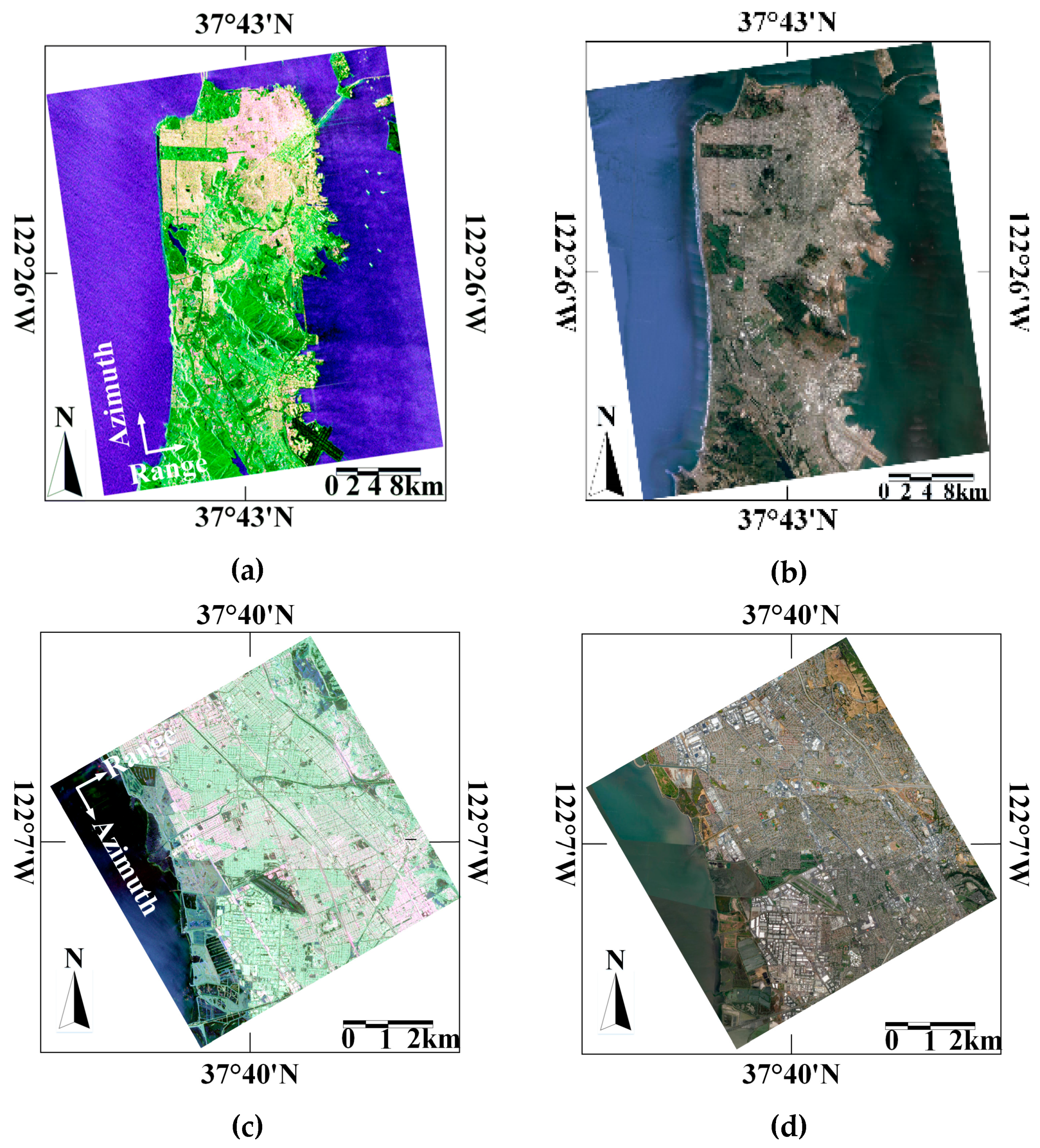
To validate the proposed building extraction method, the results reported here are derived from spaceborne and airborne PolSAR data. All original PolSAR data are single-look complex. The GF-3 C-band data was acquired in San Francisco, USA on 15 September 2017 on ascending passes with right looking direction. The pixel space is about 8.00 m × 8.00 m. The window size for the multilook processing is chosen as 7 × 7 in the ground area. The second study data is UAVSAR L-band data acquired in San Lorenzo, USA. The quad-pol data was acquired on 23 April 2010 and has a resolution with 7.20 m in the azimuth direction and 4.99 m in the range direction. The detailed parameters about the PolSAR data are listed in

Table 2. Detailed data parameters.

Sensor	Identification Code	Flight	Orbit	Incidence Angle	Height	Observation
GF-3	GF3_KRN_QPSI_005782_W122.4_N37.6_20170915	Ascending	Sun-synchronous	20°–50°	775.0 km	Right-looking
UAVSAR	Haywrd_14501_09091_004_091118_L090_CX_01	——	——	25°–65°	12.5 km	Right-looking

.

Figure 1 displays the GF-3 C-band and UAVSAR L-band data with Pauli color coding, where the red channel describes double-bounce scattering, the green channel describes volume scattering, and the blue channel describes single-bounce scattering. The corresponding optical images, which have coverage of buildings with different orientations, forests, and oceans, are also presented in Figure 1.

3.2. Extraction Results Using Model-based Decomposition

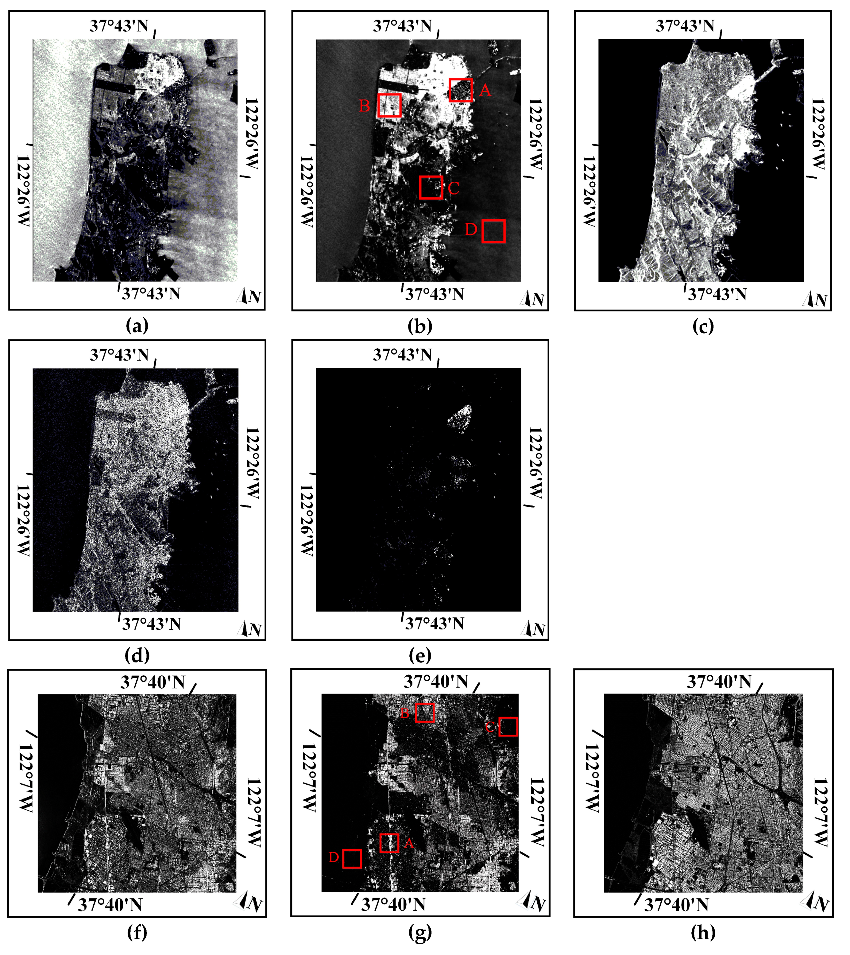
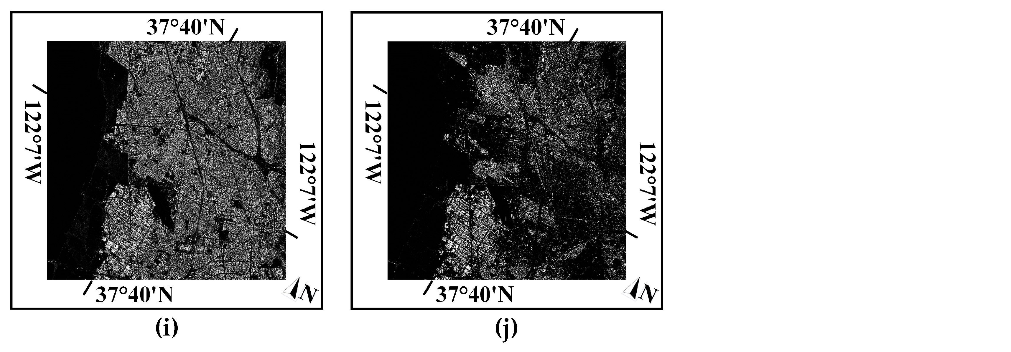
Figure 2 demonstrates the decomposition results of the R5CD, where Figure 2a–e are the surface scattering, double-bounce scattering, helix scattering, volume scattering, and the OOB scattering components, respectively. As noticed, volume scattering is the dominating contribution in the total power for natural areas, and surface scattering is identified to be dominating for the majority of the water pixels. On the one hand, from Figure 2b, it is obvious that AABs have strong double-bounce scattering power, whereas they do not exist in natural areas and OOBs. Therefore, AABs can be discriminated from the natural areas using the double-bounce scattering power. On the other hand, it can be seen from Figure 2e that the R5CD generates promising OOB scattering, which is reflected in the brightness of OOBs with different orientations. Moreover, the imperceptible OOB regions are detected, and the contours of OOBs are veraciously highlighted, especially for UAVSAR data. The above observations signify that the OOB scattering is valid and has the potential to extract OOBs. Notice that the differences between helix scattering powers of built-up areas and natural areas are very small. Therefore, it is not easy to discriminate buildings from natural areas using the helix scattering power.

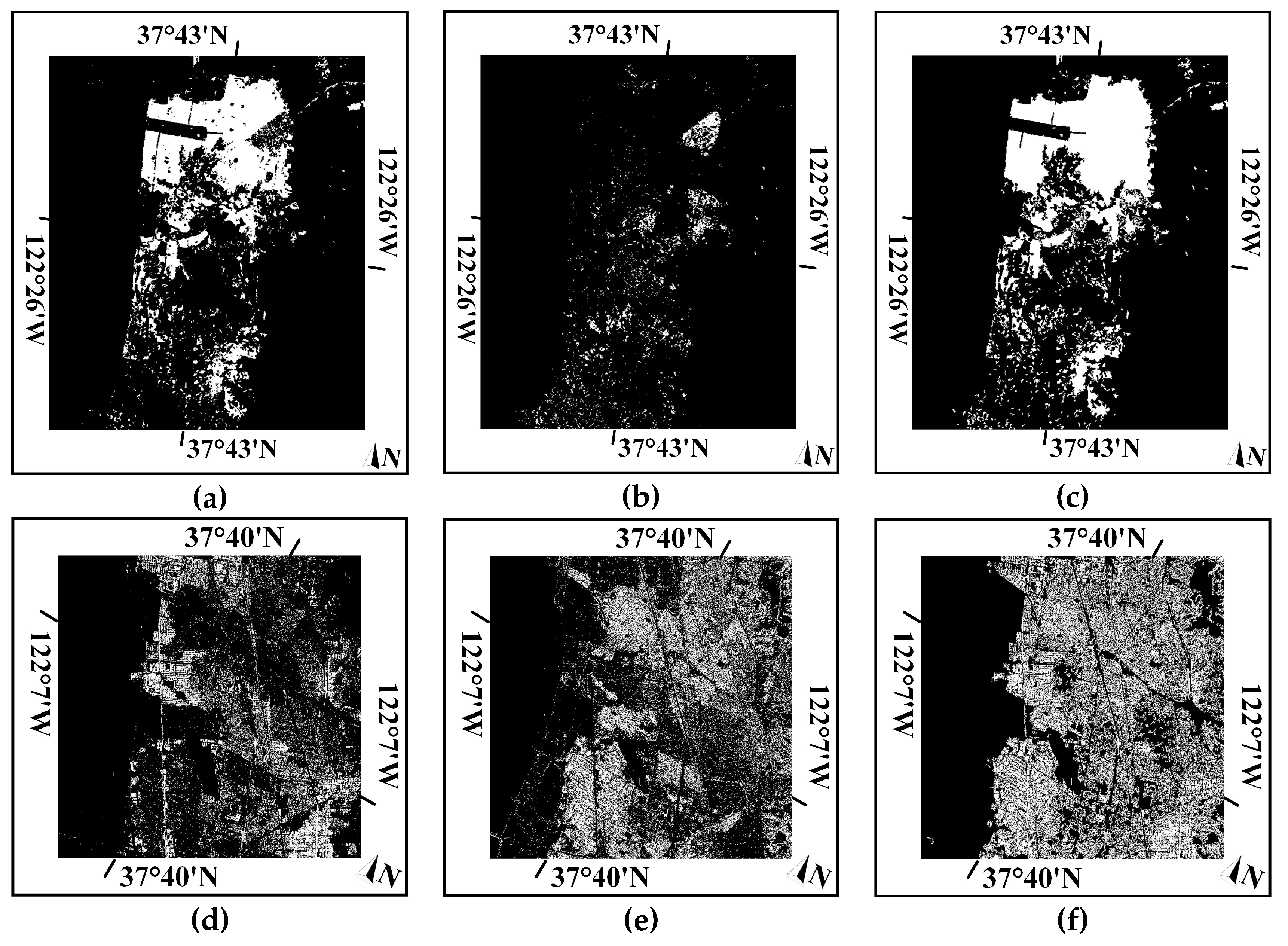
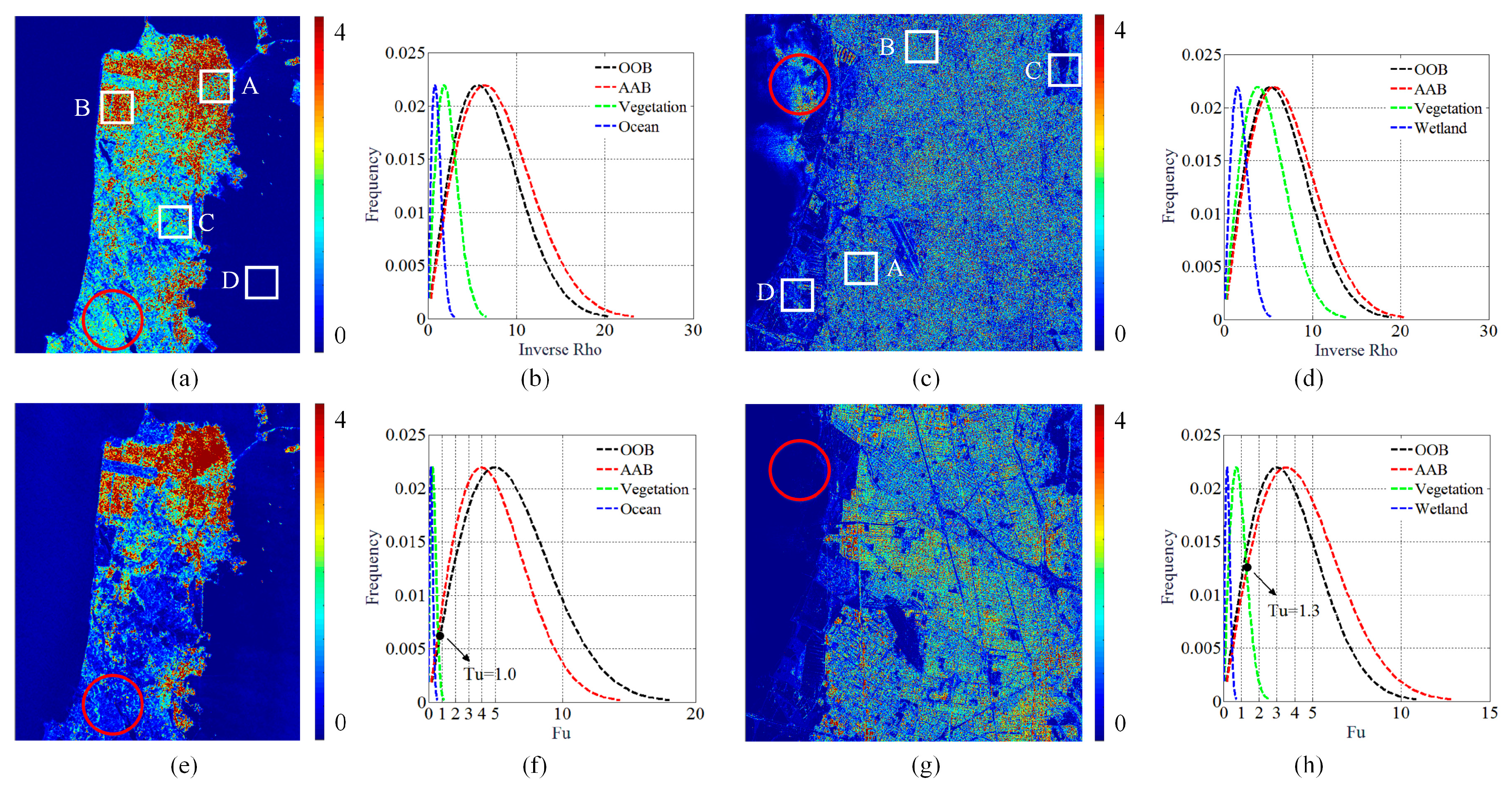
There are two thresholds involved in the R5CD-based method, i.e., $T_{\mathrm{D}}$ (threshold of double-bounce scattering power) and $T_{\mathrm{O}}$ (threshold of OOB scattering power). In order to ascertain these two thresholds, four different patches (the red rectangle areas in Figure 2) including OOBs (patch A), AABs (patch B), vegetation (patch C), and oceans/wetlands (patch D) are selected, and the averaged magnitudes of double-bounce and OOB scattering power of these patches are given in

Table 3. Averaged magnitude of scattering power for GF3 data.

	Patch A	Patch B	Patch C	Patch D
Double-bounce Scattering	0.1612	1.2198	0.0501	0.0096
OOB Scattering	0.0814	0.0002	0.0001	0.0001

and

Table 4. Averaged magnitude of scattering power for UAVSAR data.

	Patch A	Patch B	Patch C	Patch D
Double-bounce Scattering	0.1930	1.0593	0.0446	0.0098
OOB Scattering	0.0936	0.0022	0.0092	0.0015

, respectively. On the one hand, it can be found from Table 3 and Table 4 that there is an obvious segmentation of double-bounce scattering power for AABs and other areas. Accordingly, $T_{\mathrm{D}}$ is experimentally chosen as 0.5 and we believe it is suitable for both GF-3 and UAVSAR data in this work. On the other hand, since the OOB scattering mainly occurs in OOBs and vanishes in other land covers, $T_{\mathrm{O}}$ can be set to 0 directly.

According to the above thresholds, the extraction results of buildings are given in Figure 3. It is obvious that the AABs are veraciously extracted and the shapes of buildings are highlighted. The extraction results of OOBs are given in Figure 3b. Although there are a few false alarms, most of OOBs are well identified owing to the intense scattering characteristics in the OOB scattering. By combining the above two individual results, the entire extraction of buildings is generated in Figure 3c. Thereinto, some morphological processing, such as isolated point removal, hole filling, and density screening [3] are implicitly involved. Through the procedure, it can be seen that there are fewer holes and noises. Despite some falsely extracted natural targets with strong textures, buildings are mostly retained with clear shapes and contours. This explains that the double-bounce and OOB scattering power provide an effective way to extract the buildings.

3.3. Extraction Results Using Scattering Feature

In order to validate the effectiveness of the proposed scattering feature, the magnitudes of $1/\left|{\rho }_{\mathrm{HHVV}}\right|$ and $F_{\mathrm{U}}$ are given in Figure 4. Compared with $1/\left|{\rho }_{\mathrm{HHVV}}\right|$, it can be seen that both AABs and OOBs have a deeper color with $F_{\mathrm{U}}$, indicating that the buildings are better highlighted. Moreover, by incorporating the matrix elements, some natural areas, such as valleys and wetlands (outlined by the red circles) are further suppressed, thus the difference between buildings and natural areas becomes much larger. In this case, buildings can be easily discriminated from natural areas. These observations demonstrate that $F_{\mathrm{U}}$ performs much better than $1/\left|{\rho }_{\mathrm{HHVV}}\right|$ and is capable of distinguishing buildings.

To quantify the results and determine the discriminating threshold $T_{\mathrm{U}}$, the feature histograms of the same four patches are shown in Figure 4. It can be observed that buildings exhibit distinct $F_{\mathrm{U}}$ versus natural areas, which is reflected in the histogram curves of buildings, which are obviously separated from those of natural areas. In this case, the discriminating threshold can be easily determined using the histogram thresholding method (HTM) [3]. The HTM allows that if two peaks on the histogram can be found, the bottom of the valley between the peaks can be regarded as a threshold which separates the feature population into two distinctive subpopulations. Accordingly, the discriminating threshold is finally set as 1.0 and 1.3 for GF-3 and UAVSAR data, respectively (the black dots in Figure 4f,h). Notice that the histogram curves of OOBs and AABs are almost overlapped. This further explains that $F_{\mathrm{U}}$ can effectively characterize the urban scattering. Meanwhile, for $1/\left|{\rho }_{\mathrm{HHVV}}\right|$, there still exist unpleasing intersections among the histogram curves (refer to Figure 4b,d). Moreover, compared with $F_{\mathrm{U}}$, the magnitude differences between buildings and natural areas are not remarkable, which restricts its applicability.

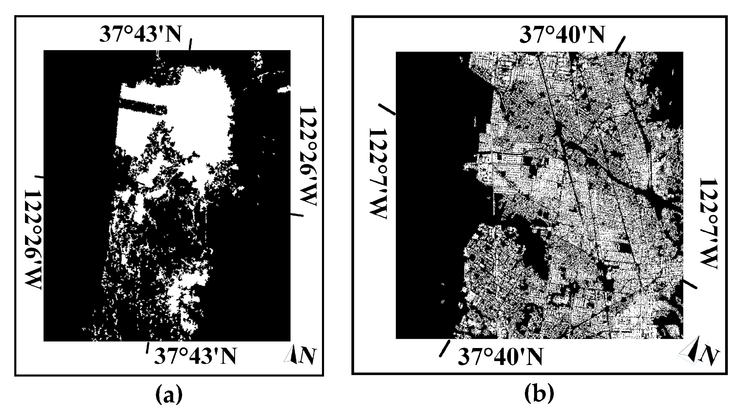
Using the discriminating threshold, built-up areas can be extracted and the results are given in Figure 5. On the whole, the feature-driven method generates visually pleasing results, reflecting in that the contours of buildings are obviously sketched and local details are well preserved. Moreover, results from GF-3 and UAVSAR data verify that the scattering feature is robust to different sensors and wavebands.

3.4. Fusion Results and Comparison

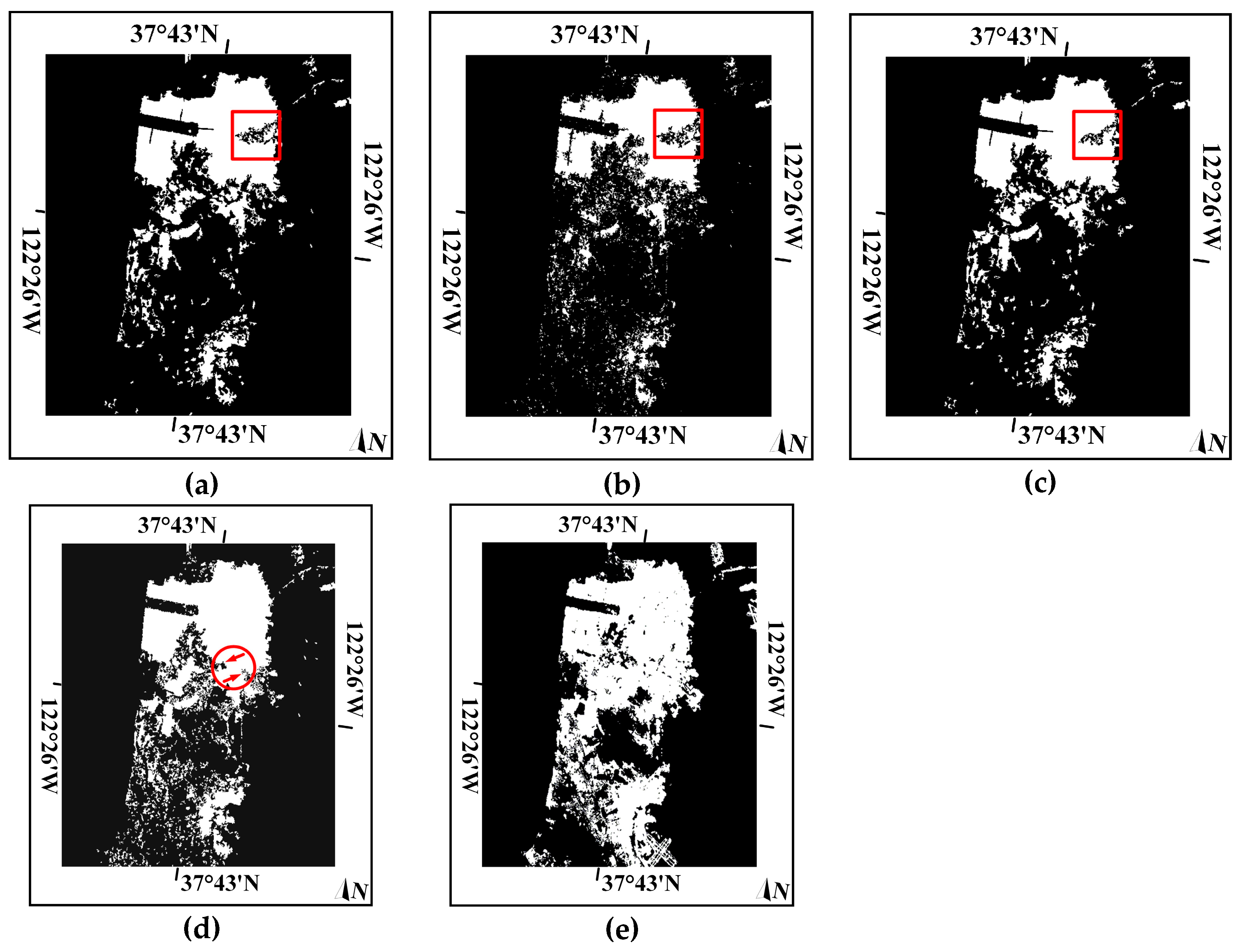
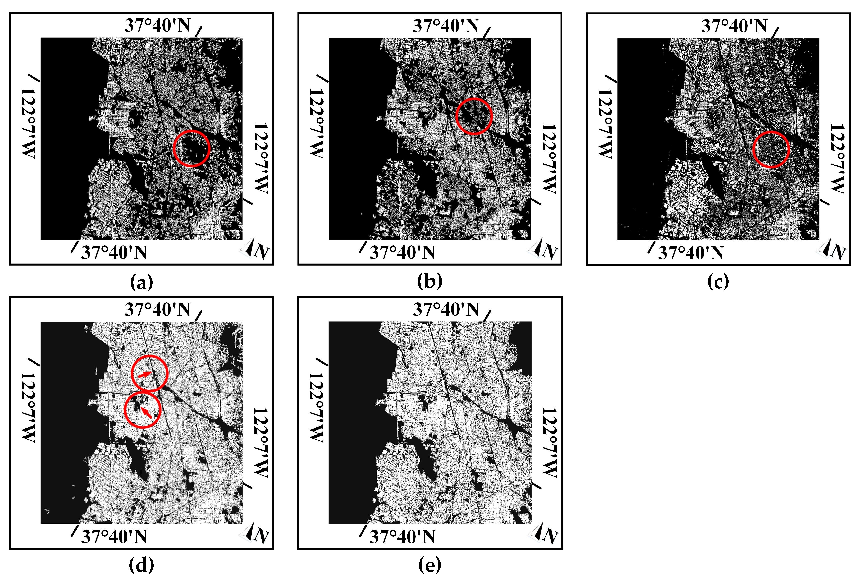
Although the two aforementioned implementations achieve relatively good extraction results, some risks needed to be noticed. On the one hand, omissions are inevitable, and they exist in different parts for different extracting processes. On the other hand, the extraction results are susceptible to the determined thresholds since the focused problem is a binary segmentation. Therefore, in order to mitigate the risks and to improve the extraction results, the HX–MRF image fusion is further applied. The fusion results for GF-3 and UAVSAR data are shown in Figure 6 and Figure 7. For comparison, three state-of-the-art methods, i.e., Azmedroub’s method [4], Xiang’s method [2], and Quan’s method [3] are involved.

Overall, all the methods are capable of detecting buildings. Nevertheless, we can see that the proposed method achieves better visual results, especially with more OOBs (red rectangle areas in Figure 6) and is able to preserve much more detailed information. Notice that the OVS is significantly present in the red rectangle areas according to the Pauli color-coded image where significant green tones can be found. However, through applying other methods, a large number of OOBs in these areas are misclassified as non-buildings. The reasons are given as follows. In Azmedroub’s method, there exists severe scattering ambiguity between OOBs and natural areas because apart from the helix scattering, the involved Yamaguchi four-component decomposition assumes that the overall cross-polarization components originate from the volume scattering, which leads to considerable misdetection of OOBs. For Xiang’s method, on the one hand, the cross-scattering model designed for OOBs is data-dependent. On the other hand, the intense cross-polarization power in OOBs actually impairs the discriminating ability of the employed polarimetric coherence. With regard to Quan’s method, the OOBs are mixed up with some natural areas since they also have very high amounts of depolarization and scattering randomness. In addition, the depolarization and scattering randomness of OOBs are susceptible to the incidence angle and wave frequency, which restrict the applicability of the extractors.

Moreover, notice that the omissions that appear in the aforementioned extraction results are eliminated (refer to the red arrows in Figure 6d and Figure 7d) and more building information is preserved after the fusion. These improvements benefit from the HX–MRF, which takes spatial correlation into consideration and produces good fusion results.

To quantitatively evaluate the extraction performance, several indices, i.e., extraction probability (EP, equivalent to producer’s accuracy (PA)), miss extraction (ME), false alarm (FA), correct rejection (CE), user’s accuracy (UA), overall accuracy (OA), and Kappa Coefficient (KC) [3] are utilized for comparison. Accuracy assessment results for GF-3 and UAVSAR data using the aforementioned methods are listed in

Table 5. Accuracy of extracted buildings from different methods.

Method	Sensor	EP/PA (%)	ME (%)	FA (%)	CR (%)	UA (%)	OA (%)	Kappa
Azmedroub (2016)	GF-3	52.86	47.14	6.43	93.57	85.40	83.57	0.623
	UAVSAR	49.81	50.19	3.94	96.06	80.20	78.32	0.586
Xiang (2017)	GF-3	46.32	53.68	5.58	94.42	81.35	80.57	0.596
	UAVSAR	50.54	49.46	3.53	96.47	82.65	79.54	0.615
Quan (2018)	GF-3	67.64	32.36	6.32	93.68	88.73	87.58	0.674
	UAVSAR	65.64	34.36	3.66	96.34	87.58	86.42	0.657
Proposed	GF-3	81.34	18.66	6.21	93.79	91.68	91.86	0.835
	UAVSAR	86.06	13.94	4.51	95.49	97.43	93.54	0.862

. We can see that the other three methods cause obvious reductions in accuracy due to the underestimated buildings. Meanwhile, the proposed method improves the overall accuracy and kappa coefficient to a great extent. For instance, compared with the results using Xiang’s method and Quan’s method, after the fusion, the kappa coefficient is, respectively, increased by 0.246 and 0.163 with respect to UAVSAR data.

From all the precedent results and analysis, it can be concluded that the proposed method, using the refined model-based decomposition and scattering feature along with the HX–MRF image fusion algorithm is the best choice for building extraction.

4. Conclusions

Traditional methods suffer from the deficiencies of inappropriate scattering modeling and non-robust feature construction for PolSAR building extraction. In this paper, we propose a robust building extraction method for PolSAR images using refined model-based decomposition and scattering variety-driven feature. The refined model-based decomposition is proposed according to the fact that the cross-polarization components are much higher than co-polarization components, which can significantly reduce the OVS and depict the OOB scattering mechanism. While for the scattering variety-driven feature, it is constructed based on the scattering variety among different land covers and is capable of highlighting the building scattering characteristics. In order to mitigate the threshold-dependent risks, the HX–MRF image fusion algorithm is adopted to further improve the extraction results. Qualitative and quantitative evaluations on different data demonstrate that the proposed method is able to extract buildings with high accuracy and outperforms other state-of-the-art methods.

References

- Zhai, W.; Shen, H.; Huang, C.; Pei, W. Buildings earthquake damage information extraction from a single post-earthquake PolSAR image. Remote Sens. 2016, 8, 171. [Google Scholar] [CrossRef]
- Xiang, D.; Tao, T.; Hu, C.; Fan, Q.; Yi, S. Built-up area extraction from PolSAR imagery with model-based decomposition and polarimetric coherence. Remote Sens. 2016, 8, 685. [Google Scholar] [CrossRef]
- Quan, S.; Xiong, B.; Xiang, D.; Zhao, L.; Zhang, S.; Kuang, G. Eigenvalue-based urban area extraction using polarimetric SAR data. IEEE J. Sel. Top. Appl. Earth Obs. Remote Sens. 2018, 11, 458–471. [Google Scholar] [CrossRef]
- Azmedroub, B.; Ouarzeddine, M.; Souissi, B. Extraction of urban areas from polarimetric SAR imagery. IEEE J. Sel. Top. Appl. Earth Obs. Remote Sens. 2016, 9, 2583–2591. [Google Scholar] [CrossRef]
- Susaki, J.; Kishimoto, M. Urban area extraction using X-band fully polarimetric SAR imagery. IEEE J. Sel. Top. Appl. Earth Obs. Remote Sens. 2017, 9, 2592–2601. [Google Scholar] [CrossRef]
- Kajimoto, M.; Susaki, J. Urban-area extraction from polarimetric SAR images using polarization orientation angle. IEEE Geosci. Remote Sens. Lett. 2013, 10, 337–341. [Google Scholar] [CrossRef]
- Wu, W.; Guo, H.; Li, X. Man-made target detection in urban areas based on a new azimuth stationarity extraction method. IEEE J. Sel. Top. Appl. Earth Obs. Remote Sens. 2013, 6, 1138–1146. [Google Scholar] [CrossRef]
- Wu, W.; Guo, H.; Li, X. Urban area SAR image man-made target extraction based on the product model and the time–frequency analysis. IEEE J. Sel. Top. Appl. Earth Obs. Remote Sens. 2017, 8, 943–952. [Google Scholar] [CrossRef]
- Sato, M.; Chen, S.W.; Satake, M. Polarimetric SAR analysis of tsunami damage following the 11 March 2011 East Japan Earthquake. Proc. IEEE 2012, 100, 2861–2875. [Google Scholar] [CrossRef]
- Xiang, D.; Tao, T.; Ban, Y.; Yi, S. Man-made target detection from polarimetric SAR data via nonstationarity and asymmetry. IEEE J. Sel. Top. Appl. Earth Obs. Remote Sens. 2016, 9, 1459–1469. [Google Scholar] [CrossRef]
- Garg, A.; Singh, D. Development of an efficient contextual algorithm for discrimination of tall vegetation and urban for PALSAR data. IEEE Trans. Geosci. Remote Sens. 2018, 56, 3413–3420. [Google Scholar] [CrossRef]
- Ji, Y.; Sumantyo, J.T.S.; Ming, Y.C.; Waqar, M.M. Earthquake/tsunami damage level mapping of urban areas using full polarimetric sar data. IEEE J. Sel. Top. Appl. Earth Obs. Remote Sens. 2018, 11, 2296–2309. [Google Scholar] [CrossRef]
- Biondi, F. Multi-chromatic analysis polarimetric interferometric synthetic aperture radar (MCA-PolInSAR) for urban classification. In Proceedings of the EUSAR 2018, Aachen, Germany, 4–7 June 2018; pp. 309–313, ISBN 978-3-8007-4636-1. [Google Scholar]
- Biondi, F. Multi-chromatic analysis polarimetric interferometric synthetic aperture radar (MCA-PolInSAR) for urban classification. Int. J. Remote Sens. 2019, 40, 3721–3750. [Google Scholar] [CrossRef]
- Salehi, M.; Sahebi, M.R.; Maghsoudi, Y. Improving the Accuracy of Urban Land Cover Classification Using Radarsat-2 PolSAR Data. IEEE J. Sel. Top. Appl. Earth Obs. Remote Sens. 2014, 7, 1394–1401. [Google Scholar] [CrossRef]
- Chen, S.W.; Wang, X.S.; Li, Y.Z.; Sato, M. Adaptive model-based polarimetric decomposition using polinsar coherence. IEEE Trans. Geosci. Remote Sens. 2013, 52, 1705–1718. [Google Scholar] [CrossRef]
- Quan, S.; Xiang, D.; Xiong, B.; Hu, C.; Kuang, G. A Hierarchical Extension of General Four-Component Scattering Power Decomposition. Remote Sens. 2017, 9, 856. [Google Scholar] [CrossRef]
- Atwood, D.K.; Thirion-Lefevre, L. Polarimetric phase and implications for urban classification. IEEE Trans. Geosci. Remote Sens. 2018, 56, 1278–1289. [Google Scholar] [CrossRef]
- Xie, Q.; Ballester-Berman, D.; Lopez-Sanchez, J.M.; Zhu, J.; Wang, C. On the use of generalized volume scattering models for the improvement of general polarimetric model-based decomposition. Remote Sens. 2017, 9, 117. [Google Scholar] [CrossRef]
- Li, H.; Li, Q.; Wu, G.; Chen, J.; Liang, S. The impacts of buildings orientation on polarimetric orientation angle estimation and model-based decomposition for multilook polarimetric SAR data in urban areas. IEEE Trans. Geosci. Remote Sens. 2016, 54, 5520–5532. [Google Scholar] [CrossRef]
- An, W.; Xie, C.; Yuan, X.; Cui, Y.; Yang, J. Four-component decomposition of polarimetric SAR images with deorientation. IEEE Geosci. Remote Sens. Lett. 2011, 8, 1090–1094. [Google Scholar] [CrossRef]
- Chen, S.W.; Ohki, M.; Shimada, M.; Sato, M. Deorientation effect investigation for model-based decomposition over oriented built-up areas. IEEE Geosci. Remote Sens. Lett. 2013, 10, 273–277. [Google Scholar] [CrossRef]
- Lee, J.S.; Ainsworth, T.L. The effect of orientation angle compensation on coherency matrix and polarimetric target decompositions. IEEE Trans. Geosci. Remote Sens. 2011, 49, 53–64. [Google Scholar] [CrossRef]
- Quan, S.; Xiong, B.; Xiang, D.; Hu, C.; Kuang, G. Scattering characterization of obliquely oriented buildingss from PolSAR data using eigenvalue-related model. Remote Sens. 2019, 11, 581. [Google Scholar] [CrossRef]
- Min, X.; Hao, C.; Varshney, P.K. An image fusion approach based on Markov random fields. IEEE Trans. Geosci. Remote Sens. 2011, 49, 5116–5127. [Google Scholar] [CrossRef]
- Freeman, A.; Durden, S.L. A three-component scattering model for polarimetric SAR data. IEEE Trans. Geosci. Remote Sens. 1998, 36, 963–973. [Google Scholar] [CrossRef] [Green Version]
- Yamaguchi, Y.; Moriyama, T.; Ishido, M.; Yamada, H. Four-component scattering model for polarimetric SAR image decomposition. IEEE Trans. Geosci. Remote Sens. 2005, 43, 1699–1706. [Google Scholar] [CrossRef]
- Xiang, D.; Ban, Y.; Su, Y. Model-based decomposition with cross scattering for polarimetric SAR urban areas. IEEE Geosci. Remote Sens. Lett. 2015, 12, 2496–2500. [Google Scholar] [CrossRef]
- Lee, J.S.; Pottier, E. Polarimetric Radar Imaging: From Basics to Applications; Taylor Francis: Boca Raton, FL, USA, 2009; pp. 85–158. ISBN 9781420054972. [Google Scholar]
- Quan, S.; Xiang, D.; Xiong, B.; Kuang, G. Derivation of the Orientation Parameters in Built-up Areas: With Application to Model-based Decomposition. IEEE Trans. Geosci. Remote Sens. 2018, 56, 4714–4730. [Google Scholar] [CrossRef]
Figure 1.
Pauli color-coded images and the corresponding optical images. (a)–(b) Gaofen-3 (GF-3) data. (c)–(d) uninhabited aerial vehicle SAR (UAVSAR) data.
Figure 2.
Decomposition results of the refined five component decomposition (R5CD). (a)–(e) Surface, double-bounce, volume, helix, and oblique orientation (OOB) scattering for GF-3 data, respectively. (f)–(j) Surface, double-bounce, volume, helix, and OOB scattering for UAVSAR data, respectively.
Figure 3.
Extraction results using the double-bounce and OOB scattering powers. (a)–(c) Extraction of buildings approximately aligned with the flight trajectory (AABs), OOBs, and built-up areas for GF-3 data, respectively. (d)–(f) Extraction of AABs, OOBs, and built-up areas for UAVSAR data, respectively.
Figure 4.
Magnitudes of proposed scattering feature and histograms of selected patches. (a)–(b) The magnitudes and histograms of for GF-3, respectively. (c)–(d) The magnitudes and histograms of for UAVSAR, respectively. (e)–(f) The magnitudes and histograms of for GF-3, respectively. (g)–(h) The magnitudes and histograms of for UAVSAR, respectively.
Figure 5.
Extraction results using the scattering feature. (a) GF-3 data. (b) UAVSAR data.
Figure 6.
Comparison of different building extraction methods for GF-3 data. (a) Azmedroub’s method, (b) Xiang’s method, (c) Quan’s method, (d) the proposed method, (e) ground truth.
Figure 7.
Comparison of different building extraction methods for UAVSAR data. (a) Azmedroub’s method, (b) Xiang’s method, (c) Quan’s method, (d) the proposed method, (e) ground truth.