Article

Mapping Invasive Phragmites australis in the Old Woman Creek Estuary Using UAV Remote Sensing and Machine Learning Classifiers

1
Department of Geology, School of Earth, Environment and Society, Bowling Green State University, 190 Overman Hall, Bowling Green, OH 43403, USA
2
Ohio Department of Natural Resources, Old Woman Creek National Estuarine Research Reserve, Huron, OH 44839, USA
3
Fireland Coastal Tributaries, Erie Soil and Water Conservation District, Sandusky, OH 44870, USA
*
Author to whom correspondence should be addressed.
Remote Sens. 2019, 11(11), 1380; https://0-doi-org.brum.beds.ac.uk/10.3390/rs11111380
Submission received: 29 March 2019 / Revised: 26 May 2019 / Accepted: 6 June 2019 / Published: 10 June 2019

Abstract

:
Unmanned aerial vehicles (UAV) are increasingly used for spatiotemporal monitoring of invasive plants in coastal wetlands. Early identification of invasive species is necessary in planning, restoring, and managing wetlands. This study assessed the effectiveness of UAV technology to identify invasive Phragmites australis in the Old Woman Creek (OWC) estuary using machine learning (ML) algorithms: Neural network (NN), support vector machine (SVM), and k-nearest neighbor (kNN). The ML algorithms were compared with the parametric maximum likelihood classifier (MLC) using pixel- and object-based methods. Pixel-based NN was identified as the best classifier with an overall accuracy of 94.80% and the lowest error of omission of 1.59%, the outcome desirable for effective eradication of Phragmites. The results were reached combining Sequoia multispectral imagery (green, red, red edge, and near-infrared bands) combined with the canopy height model (CHM) acquired in the mid-growing season and normalized difference vegetation index (NDVI) acquired later in the season. The sensitivity analysis, using various vegetation indices, image texture, CHM, and principal components (PC), demonstrated the impact of various feature layers on the classifiers. The study emphasizes the necessity of a suitable sampling and cross-validation methods, as well as the importance of optimum classification parameters.

1. Introduction

The loss and degradation of coastal wetland vegetation due to anthropogenic activities and climatic changes motivate researchers to seek sustainable and efficient management strategies. The ability to understand the dynamics of wetland vegetation is hindered by access limitations due to the risk of damaging habitats and species, fine scale variations of vegetation and hydrology [1]. Mapping, identification, and classification of plant types and species are vital in planning, restoring, and managing coastal wetlands. Capturing the distribution of alien plant species and particularly controlling the invasive ones is a significant challenge that wetland managers and policy makers face [2]. Early identification and accurate information about the distribution of invasive species are necessary to anticipate, assess, control, and mitigate their negative impacts on the existing ecosystem health [3,4]. These alien invasive plants make an impact on the composition and function of both natural and managed ecosystems with substantial economic cost in response to losing or degrading land use and eradication efforts [5,6]. The success of an invasion of alien species depends on the plant’s ability to invade a new region and the susceptibility of the ecological system which is invaded [7]. Blackburn et al. [8] dissect the plant invasion process into several stages, namely, transport, introduction, establishment, and spread. During this invasion process, an alien species should pass sequential barriers (e.g., geographical, survival, reproductive, and dispersion) to enter, survive, and spread in a new territory. The invasive species which successfully pass the barriers, compete for space and nutrients in the ecosystem and alter the soil structure and nutrient cycles [9,10].
Phragmites australis (later in the text as Phragmites) is one of the most widespread plants globally and it is seen as a threat to wetlands worldwide [11]. Phragmites is a tall erect perennial grass that aggressively dispersed over eastern North America during the last two decades [10,11,12,13]. The Phragmites haplotype M, which was introduced from Eurasia, has been rapidly replacing its native types and other local plants in most North American wetlands [14]. They disperse to new areas predominantly by seed germination and spread asexually by stolons or rhizomes around the existing patches [15,16]. Dense Phragmites patches reduce the quality of habitats for fish and bird species, especially due to drying out the littoral zones and affecting sedimentation [17,18].
Remote sensing is a widely used technology that is capable of providing spatial and temporal information about invasive species in wetlands [14]. As remote sensing data analyses become more advanced, data integration methods such as multi-sensor and temporal data fusion become prevalent in enhancing the extraction of information. The tradeoffs among spatial extents, and spatial and spectral resolutions of imagery, affect the quality of information. Several studies fostered hyperspectral data with their continuous spectral band configuration, which provide more details on the spectral characteristics of plants than multispectral imagery [19]. For example, the Compact Airborne Spectrographic Imager (CASI)-1500 and the Airborne Hyperspectral Scanner (AHS) sensors, used to identify the invasive plant Spartina densiflora in a wetland, showed promising results using four spectral target detection algorithms [20]. The hyperspectral imagery of the Airborne Visible/Infrared Imaging Spectrometer (AVIRIS) was found to be capable of mapping invasive plants distributed over large areas with high overall accuracy [21], although another study suggested that AVIRIS data were not appropriate to map small and highly heterogeneous areas comprised of invasive plants due to the inadequate spatial resolution [22].
In recent years, many studies have stated the necessity of high spatial resolution imagery to map wetlands to compensate for the spectral similarity among plant types [22,23,24,25]. The commercially available high-resolution (sub-meter spatial resolution, e.g., WorldView and QuickBird) satellite sensors provide more spatially detailed images with a small geometric distortion [26]. A classification study conducted to distinguish emergent invasive plants in a diked wetland in the western basin of Lake Erie using QuickBird (2.4 m spatial resolution) images demonstrated the ability of this sensor to distinguish long and narrow patches of invasive plants (Phragmites australis and Typha) [27], while the hyperspectral Hyperion imagery (30 m spectral resolution) was not successful in identifying the small and linear arrangements of Phragmites australis in the west coast of the Green Bay shoreline [28]. Distribution maps of the invasive plant Hakea sericea monitored with WorldView 2 images showed a high overall accuracy [29] although the maps were not suitable to detect Hakea sericea at early stages of invasion due to the insufficient spatial resolution of the images. A major drawback of using a commercially available high-resolution satellite data is the high cost of the images and pre-ordering process related to data acquisition. In recent years, the use of an unmanned aerial vehicle (UAV) for detection of invasive species is seen as an economical way of obtaining remote sensing images at any desired time.
UAVs can acquire very high spatial resolution data (~10 cm) with a user defined flight plan and flexible revisit time [30]. In addition, UAVs allow flying at different heights which can be utilized to adjust the spatial resolution of the images [31]. Consequently, very high spatial resolution imagery captured by UAVs became practical in natural resource management to monitor invasive plant species in several different ecosystems [31,32,33]. Several recent studies [22,31,32,33,34,35,36] have proved that the use of UAV-borne remote sensing is an effective method to classify vegetation. Pande-Chhetri [37] used UAV data to classify wetland vegetation with pixel-based and hierarchical object-based classification approaches. The object-based classification with a support vector machine (SVM) classifier resulted in the highest overall accuracy in the study. While searching for the optimum method to discriminate invasive Lantana camara from the forested landscape, Nipadhkar et al. [32] found that the object-based classification provided the better visual organization of plant classification and performed satisfactorily. Müllerová et al. [22] emphasized the importance of the temporal flexibility in data collection with UAVs over Pleiades satellite images in monitoring invasive plants. The best classification accuracy for invasive Heracleum mantegazzianum (giant hogweed) was reached during the flowering time using the object-based classification approach. This study highlighted the importance of collecting data at the correct time of the growing season. Samiappan et al. [33] used five band UAV images to map invasive Phragmites australis in a tidal marsh to identify the impact of features such as normalized difference vegetation index (NDVI), soil adjusted vegetation index (SAVI) and morphological attribute profiles (MAPs). Further, a canopy height model (CHM) generated using the digital terrain model (DTM) and the digital surface model (DSM) derived from UAV data becomes useful among remote sensing researchers [38,39,40]. The use of UAV and light detection and ranging (LiDAR) derived CHM was identified as an important feature to improve the accuracy in vegetation classification [41].
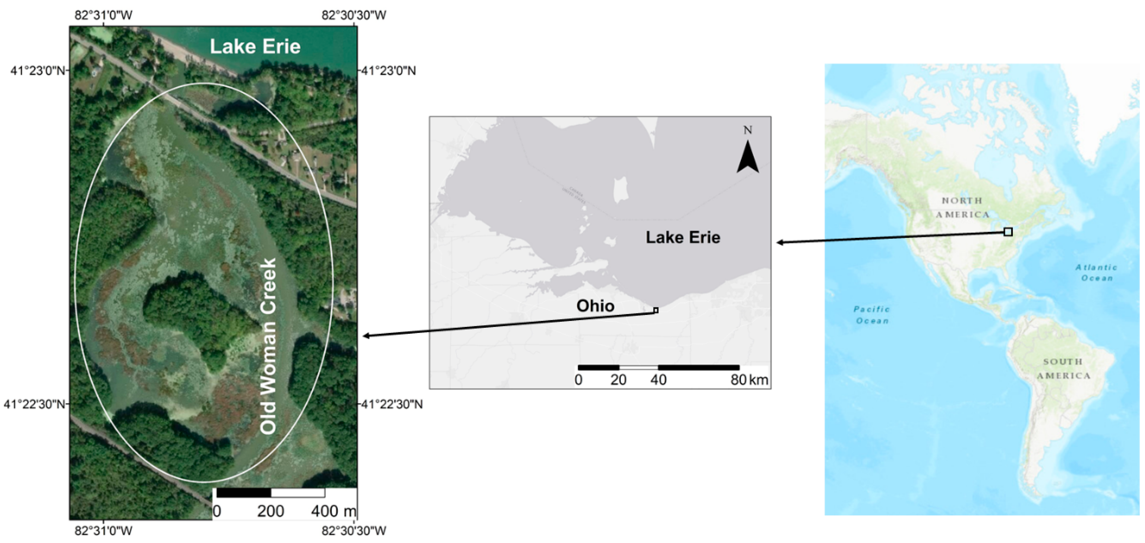
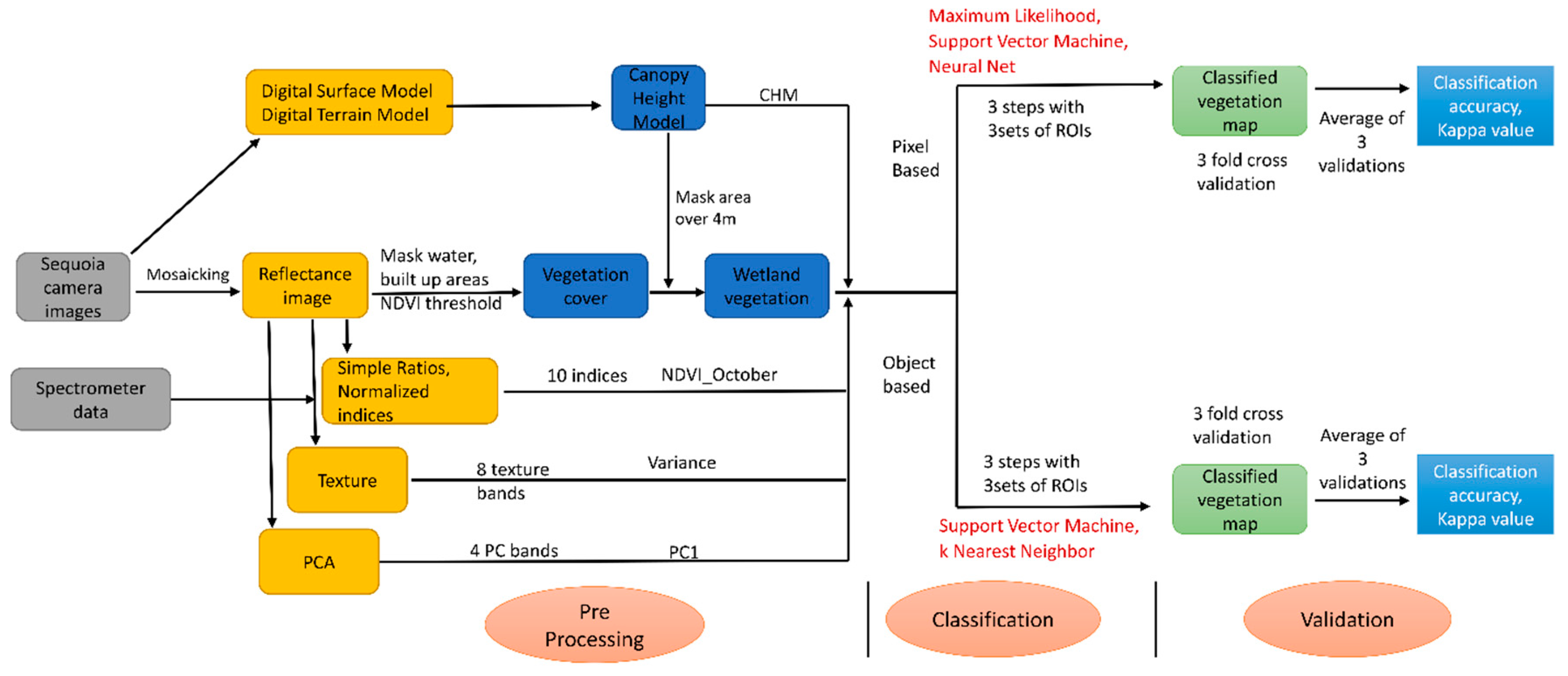
The goal of this study is to explore the effectiveness of UAVs in mapping Phragmites, in the Old Woman Creek (OWC) estuary, located in the Lake Erie region in Ohio, using machine learning (ML) classifiers: k-nearest neighbors (kNN), support vector machine (SVM), and neural network (NN), and their possible advantages over the more traditional approach, maximum likelihood classifier (MLC) using pixel- and object-based classification methods. The objectives of the study are: (i) identify the best machine learning classification algorithm to detect Phragmites as well as to compare it with the parametric MLC; (ii) explore the impact of different feature layers derived from the UAV data on the performance of the classifiers, including various vegetation indices from mid- and late-growing season, image texture, principal components (PC) and the canopy height model (CHM); (iii) assess the optimum use of sample design and cross-validation sampling techniques. The results of this study will be helpful to understand the dispersion of Phragmites in the OWC estuary and to plan the eradication strategies efficiently.

2. Materials and Methods

2.1. Study Area

The study took place at Old Woman Creek (OWC), a natural estuary located at the southernmost point (41°22′N, 82°30′W) of the Lake Erie shoreline near the town of Huron, Ohio (Figure 1). The OWC extends approximately 2.1 km2 from the southern shore of Lake Erie [42]. It is one of (the) 29 areas protected under the National Estuarine Research Reserve System (NERRS), and it is known for high biodiversity and unique water regime [43]. The barrier beach controls the connection between the OWC estuary and Lake Erie. It closes the mouth of the beach during times of high rainfall and opens it during summer when the water level changes by seiches and storm surges of Lake Erie [42,44]. The extent and duration of the water level fluctuation directly influence the variety of vegetation in the estuary [43].
The plant life forms in OWC range from terrestrial plants, which tolerate occasional submergence, to the plants completely adapted to survive only in an aquatic environment [44]. Over 800 terrestrial and aquatic species of vascular plants have been identified in its watershed [46]. While increased water levels transform several former wetlands to shallow open-water areas with a small amount of aquatic vegetation [42], the reduction of the water level, on the other hand, results in the increase of the distribution of invasive plants in OWC [43]. Currently, Phragmites is observed as the most dominant invasive plant type in OWC [47] and Lythrum salicaria (purple loosestrife), Myriophyllum spicatum (Eurasian water-milfoil), Limnobium laevigatum (frogbit), and Alloaria petiolata (garlic mustard) are also being observed. Phragmites spreads rapidly toward the south along the banks of the creek during low water level periods [44]. Dense patches of invasive Phragmites were observed near the estuary mouth and on both sides of the road running through the site (Figure 1). Phragmites is often seen within several cattail patches on the site. The study site is surrounded by tall trees on the banks of the estuary. The star-shaped island covers a larger area of the study site, and the rest is covered with aquatic plants and water. The aquatic area is mostly covered with floating and emerging plants. Access is restricted to most of the south, west, and southwest sections of the estuary with densely grown, submerged, and floating plants (Figure 1).

2.2. Field Data Collection

UAV imagery over the study site was acquired on two days: 8 August 2017 (mid-growing season), and 18 October 2017 (late-growing season). The former image was the main image used in the process of classification supported by vegetation indices derived from the October image. The UAV used in this study was a SenseFly eBee Ag model [48]. The weight of the eBee is approximately 700 g and the flight time was between 25 and 30 min. Flight planning was performed with the eMotion 2 [49] software package. The ceiling of the flights was set at 120 m. Lateral and longitudinal overlaps of the flight plans were set to 75%. The flight radius was set to 880 m. The flights were carried out in clear weather conditions with wind speed between 9 and 18 km h−1.
A Parrot Sequoia camera attached to the UAV, with green (G) (530–570 nm), red (R) (640–680 nm), red edge (RE) (730–740 nm), and near-infrared (NIR) (770–810 nm) spectral bands, was used to acquire the images. The spatial resolution of the images was 13.90 cm. One additional flight was conducted using the SONY DSC WX 220 RGB (SONY Corporation of America, New York, USA) camera on the same day, 8 August 2017. The purpose of acquiring images with the RGB camera was to use it as a visual aid to identify plants in the estuary, which were clearly distinguished with better spatial resolution of 3.43 cm, as well as in the process of validation. The RGB camera was not used in the classification process as it lacked the NIR band.
In addition to the UAV data acquisition, a handheld PSR 3000 Spectral Evolution spectroradiometer was used to collect in situ spectral measurements of five wetland plants of interest: lotus, lily, duckweed, Phragmites, and cattails in the period from 31 July 2017, to 21 August 2017. The spectroradiometer covers the wavelength range from 350 nm to 2500 nm. Spectral resolutions of the instrument are 3 nm from 350 nm to 700 nm, 8 nm from 700 nm to 1500 nm, and 6 nm from 1500 nm to 2100 nm of the spectral range [50].
To recognize critical regions on the hyperspectral signatures and to select vegetation index which would possibly enhance the process of classification, thirty averaged spectral measurements, conducted at approximately 0.5 inches above the leaves, were taken over various locations for each selected plant type. DARWin SP [50] was used to process the data.

2.3. Study Workflow

2.3.1. Image Pre-Processing

Pre-processing of UAV images included geotagging and mosaicking of the raw images as well as generation of digital surface model (DSM) and digital terrain model (DTM). UAV images taken by the cameras were geotagged with eMotion 2 software using the log files generated by eBee during each flight. The geotagged images were orthorectified and mosaicked as reflectance images using Pix4Dmapper Pro [51]. The projected coordinate system was set to WGS 1984 UTM Zone 17 N. In order to combine data from different dates, the Sequoia generated multispectral image taken on 18 October was georegistered to the image taken on 8 August. The registration was performed with the image registration workflow tool of ENVI 5.4 using six reference points on each image. The RMSE error between the two images was 1.32 pixels.
The area with wetland vegetation was extracted with two masking steps. First, the areas that consisted of water and built-up features were masked by using NDVI and its threshold of 0.22. Second, the vegetated area with the height over 4 m was masked to remove trees and tall vegetation. Among the selected wetland plant types, Phragmites are the tallest plant type which grows up to maximum heights of 3–3.5 m in the estuary.

2.3.2. Derived UAV Products

Several feature layers were derived from UAV products: various band indices, texture images, CHM, and PC. They were added to the original UAV bands (G, R, RE, and NIR) in the process of classification one by one to explore if and how each layer might enhance the process. The purpose of this sensitivity analysis was to select one feature layer within each feature group, which produced the lowest errors of omission for Phragmites, and then to combine them and monitor the trends and possible improvements in accuracy assessments. The goal was to reduce not only the overall accuracy, but also the omission errors for Phragmites, an important criterion for successful eradication of Phragmites.

Band Indices

Six simple band ratios and three normalized band indices were selected based on the differences between the field hyperspectral signatures of the five wetland plants (Table 1). The band indices were calculated for the images taken on both days, 8 August and 18 October, to explore the effect of their temporal changes on classification. Due to the different phenology state of plants and, thus, better separability of spectral signature between the plants, data acquired in the late-growing season, may enhance the classification process [22].

Image Texture

Chavez [59] showed that the spatial distribution of spectral variability of vegetation is higher within the NIR band than within the visible (RGB) spectral region over an area. Thus, the NIR band of the 8 August image was used to calculate the texture values in the current study. The gray level co-occurrence matrix (GLCM) tool within ENVI 5.4 software (Harris Geospatial Solutions, Broomfield, Colorado, USA) was used to calculate eight GLCM measures: mean, contrast, homogeneity, second moment, correlation, dissimilarity, entropy, and variance. Since the focus was to map Phragmites, which is a thin, erect plant, the kernel size was set to 3 × 3 pixels.

Principal Components

The principal component transformation was performed with the forward principal component analysis (PCA) rotation tool. PCA converts the original multispectral bands to a new set of bands producing the highest variance in the first PCA band, while the variance is reduced sequentially from band 1 to band 4 [60].

Canopy Height Model

DSM represents the elevations of the objects on the ground and DTM indicates the elevation of the bare land [61]. The canopy height model (CHM) was created by subtracting DTM from DSM using Bandmath tool in ENVI 5.4. CHM indicates the absolute heights of the objects within the image extent. The spatial resolutions of DSM and DTM created with Pix4D were 13.04 cm and 65.02 cm. Thus, both DSM and DTM were resampled to 13.90 cm spatial resolution to keep the pixel size consistent between images.

2.3.3. Classification

Image classification was performed using pixel- and object-based classifiers. The ENVI 5.4 software package was used for pixel-based classifications, and Trimble eCognition Developer 9 [62] was used to perform object-based classifications. All image bands were scaled to the pixel values ranging between 0 and 100 before the classification to be able to generate meaningful objects [63]. The images were classified into five classes: Phragmites, cattails, lotus, lily, and duckweed. In this study, the MLC, SVM, and NN classifiers were used in the pixel-based approach, and two classifiers, SVM and kNN, were used in the object-based method. All algorithms used in the study, except the parametric MLC, are non-parametric ML classifiers and make no assumptions on the data distribution. The ML classifiers were compared to the traditional pixel-based MLC to explore possible advantages of ML algorithms [64]. The feed forward NN classification was performed by the Neural Net function. The values were selected as suggested in Ndehedehe [65]. The NN classifier was selected as it could learn complex patterns in training data, generalize the noise of data, and perform classification with a lower number of samples [66]. The SMV classifier was used within both the pixel- and object-based methods. Radial basis function (RBF) was used with the SVM classifier as it performed better than other kernels [67,68]. Several studies suggested that SVM classifies image accurately with a small number of training samples [69,70,71]. The kNN classifier is a widely used object-based classification algorithm and one of the simplest ML classifiers.
The parameters of the non-parametric classifiers were optimized before the process of classification [64,69] (Table 2). Within the object-based classification, the image was first separated into segments (object) with 10, 20, 40, 50, 75, and 100 scale parameters and then classified into the five classes as explained below [72]. The segment boundaries were examined after each segmentation to ensure that segments consisted of only one plant type. After a visual comparison among segmentations, the best scale parameter for segmentation of the image was identified as 40. Several segmentations were performed with fixed 40 scale parameter to find the best compactness parameter of 0.5 which resulted in the most realistic shapes of segment boundaries. The higher value of the shape parameter decreases the consideration of spectral information during segmentation. Consequently, the shape parameter was set to 0.1 to maximize the consideration of the band spectral information. The weight values for each image layer were set to 1, to consider all the bands as equally important in the classification.
The UAV image acquired on 8 August 2017 was classified at three different levels of complexity using the proposed classifiers considering: (i) the four original bands (G, R, RE, NIR) (4sq); (ii) the sensitivity analysis where one feature layer at a time was added to 4sq, including information from the October image; and (iii) the combination of representative feature layers with the best performance added to 4sq. The overall classification accuracy, kappa value, and errors of omission and commission for the Phragmites class were used to compare the classifiers. The optimum set of accuracy parameters for each classifier was decided to be the one with high overall accuracy (OA) and with the least error of omission, a critical point for eradication of invasive species and wetland management. The workflow is shown in Figure 2.

2.3.4. Sample Design

Stehman and Czaplewski [73] defined the sampling design as the protocol that should be followed during the selection of sampling units as training and validation regions of interest (ROIs). A stratified random sampling design was used to create training and validation data sets in this study. Several patches were chosen for each plant type, and then ROIs were randomly selected within each patch. The ROIs were created based on the GPS coordinates recorded in the field and additional ROIs were visually selected from the RGB image.
The selection of ROIs started with one pixel, and the rest of the pixels was calculated by the Grow ROIs from Neighboring Pixels function, a spatially smooth technique [73]. The one-pixel ROIs were allowed to grow, using the criteria of the within-two standard deviations of pixel values, up to the maximum number of eight neighboring pixels [74]. The ROIs consisted of at least four pixels after applying the Grow ROIs function. The number of training data could heavily impact the classification accuracy [75]. In this study, the number of ROIs for each plant type was selected according to the proportional area covered with each plant type. Forty-eight ROIs were selected for each lotus, lily, and cattails, as these plants were most abundant. The number of ROIs selected for duckweed and Phragmites were 39 and 33, respectively.
In order to minimize the uncertainties that were observed in this study while examining the impact of different sampling designs and different numbers of ROIs on the overall accuracy, the three-fold cross-validation approach was used to assign ROIs to the classification and validation processes. The spatial distribution of ROIs was kept equal when splitting the ROIs into three sets. Two sets of ROIs were used as classification data and the remaining set as validation data through the iterative process. The classification accuracy results were averaged after the process. Although the k-fold cross-validation is computationally extensive, it is most suitable when the study aims to find the precise error rates of the classifiers [76]. This method compensates for errors that could arise due to a smaller number of samples used in the classification and validation.

3. Results

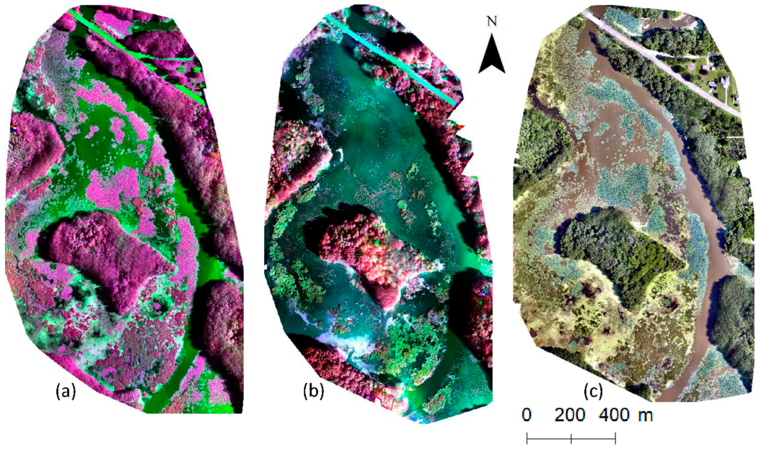
The image mosaics created for the study area for August (called 4sq hereafter) and October using Sequoia camera (Figure 3a,b) show senescence of some wetland plants in October. This temporal variation is critical to derive NDVI from the October image (NDVIOct) and to improve the classification results, as shown below. The RGB image (Figure 3c) shows more detail and was useful as supplementary data in the ROI collection and validation processes. Most of the shaded areas, especially in the Sequoia images, are removed in the process of masking, as most of the shadows were over water, roads or within trees.
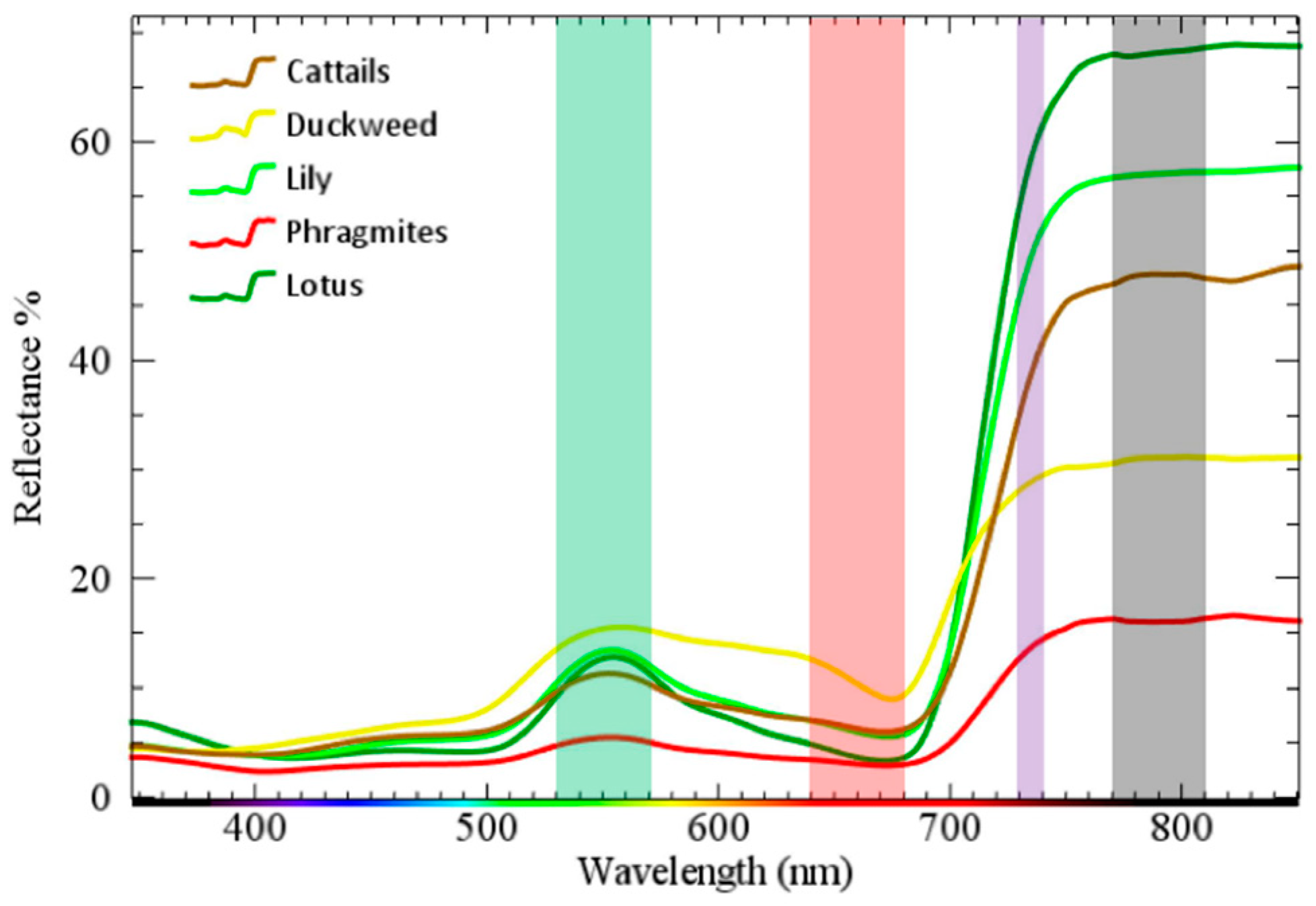
Distinctive differences between the plants’ spectral signatures, collected by the hand-held spectroradiometer, are observed in NIR and RE spectral ranges where lotus exhibits the highest and Phragmites the lowest values (Figure 4). In the green spectral region, the spectral signal is similar between cattails, lotus, and lilies, somewhat higher for duckweeds and relatively low for Phragmites. A similar trend is observed in the red spectral range except for lotus whose reflectance decreases and becomes almost identical to the reflectance of Phragmites. The Phragmites signature is relatively distinctive from other plants as it keeps similar values in red and green and the lowest values in NIR/RE regions, which is expected given the earthy color of the plant. In particular, the similarity of the reflectance in the red and the dissimilarity in the NIR bands between Phragmites and lotus is in accordance with our findings shown below that NDVI index perform best to differentiate Phragmites and lotus.

3.1. Pixel-Based Classification

The best results for 4sq are attained with the SVM classifier (OA = 90.47%) and then with MLC and NN are 88.23% and 84.58%, respectively (Table 3). While OA reaches relatively high values for all classifiers, the class classification accuracy (i.e., correctly classified percentage per class) is considerably lower for Phragmites and lotus than other plants, 82.42% and 82.35%, respectively (Table 3). It is observed from the results that Phragmites are commonly misclassified as lotus and to a lesser extent as cattails, 15.99% and 1.59%, respectively, and that 1.15% of cattails and 8.89% lotus are classified as Phragmites. The errors of commission (CE) and omission (OE) are relatively high for Phragmites (CE = 15.68% and OE = 17.58%, respectively).
Although differences between spectral signatures are observed in Figure 4, the UAV-derived NDVI values between Phragmites, cattails, and lotus do not differ significantly from each other in August (Table 4). Thus, as expected, the NDVI feature layer from August was found not to be beneficial to the classifications and it was excluded from further analysis. The reduction in NDVI from August to October is greater for cattails and lotus compared to Phragmites as suggested by the Tukey–Kramer test (Table 4). Nevertheless, NDVIOct is statistically different among the plants and it improves the classifications (Table 5). This seasonal trend was observed for all vegetation indices as shown in Table 5.
The SVM accuracy parameters for the sensitivity analysis of classification, where the feature layers (band indices, texture, CHM, and PC bands) are stacked to the 4sq image one by one, are shown in Table 5. Out of all indices used in the study, NDVIOct performs best with the highest overall accuracy of 93.43%, the lowest error of omission of 5.56%, and second lowest error of commission of 4.86%.
Just a slight improvement of the OA values is observed when texture information is added to 4sq. While the errors of commission are considerably decreased down to 2.08% for several texture layers, the errors of omission are increased for most of them. Variance is the only layer that results in a somewhat, but insignificantly, lower error of omission (OE = 17.24%) when compared to the 4sq case (OE = 17.58%, see Table 3), and thus, it was selected as the texture layer with the best contribution to the classification. CHM performs well, resulting in high OA (OA = 93.59%) and relatively low errors of commission and omission (1.75% and 9.53%, respectively). PCs do not contribute considerably to the classification of Phragmites. PC1 results in somewhat, but not considerably, lower error of omission (OE = 15.52%) than observed in the 4sq case (OE = 17.58%, see Table 3).
In summary, the sensitivity analysis suggests that each additional layer to 4sq increases OA (except PC3 and PC4), although in many cases the increase is negligible. The lowest error of omission is reached with NDVIOct; the second lowest error of omission for the Phragmites class is achieved by using the CHM layer; and then negligibly lower by using PC1 and Variance (Var) layers, respectively.
The resulting classification accuracies based on the combination of the selected feature layers for the pixel-based classifiers are shown in Table 6. Among the three pixel-based classifiers, when both NDVIOct and CHM layers are added to 4sq, the highest overall classification accuracy with the value 94.80% and the highest kappa value of 0.93 are achieved with the NN classifier. The overall accuracy and kappa values decrease when adding more layers (PC1 and Var) to the NN and SVM classifiers. The maximum overall accuracy for MLC is reached for the 4sq+NDVIOct combination (93.46%), and it decreases to 92.92% when CHM is added. The kappa values follow the trend. Any additional layer either decreases the accuracy or produces non-realistic values for MLC (Table 6). The ML methods do not yield considerably better results than MLC.
Similarly, the class classification accuracies for Phragmites increase for all classifiers when NDVIOct is added and further increase when CHM is included. Maximum values are reached for the 4sq+NDVIOct+CHM combination for all three classifiers. The errors of omission are significantly lowered with NDVIOct and further reduced by adding CHM for all classifiers. The lowest error of omission is achieved with the 4sq+NDVIOct+CHM combination using NN (OE = 1.59%). MLC performs well with the lowest error of commission among all classifiers and somewhat higher error of omission than NN (CE = 2.22%; OE = 3.17) for the same (4sq+NDVIOct+CHM) combination (Table 6; Figure 5). The additional PC1 and Var layers do not improve the performance of any of the classifiers.

3.2. Object-Based Classification

The segmented images, generated prior to the object-based classification, were classified following the same band combinations. The results of the classifications are shown in Table 7, for the overall and class accuracy, respectively.
SVM performs slightly better than the kNN for all layer combinations but overall, both classifiers showed lower OA than any of the pixel-based classifiers. The addition of the NDVIOct to 4sq improves the OA values for SVM by approximately 2% (from 87.69% to 89.23%), while the overall accuracy for kNN is reduced by 2% (from 86.92% to 84.62%). Similar to the pixel-based classifications, the highest overall classification accuracy was achieved with SVM for the band combination of 4Sq+NDVIOct+CHM. Although the differences are not significant, the combination of more bands does not improve the overall accuracy and kappa values, with an exception when PC1 is added to kNN.
The combination of NDVIOct+CHM layers reduces the error of commission for the Phragmites class from 28.57% to 3.57% with SVM and from 2.13% to 1.78% with kNN. Similar to the pixel-based classification approach, the minimum errors of omission are observed for the 4sq+NDVIOct+CHM combination for SVM (from 25.00% to 5.32%), and no further reduction is observed by adding the layers (Table 7). The 4sq+NDVIOct+CHM is the combination that represents the cutoff point where the errors of omission and commission do not improve after adding additional layers. The positive attribute of kNN is that this classifier exhibits lower errors of commission while SVM is more consistent and predictable in reducing the errors of omission (Table 7). Both classifiers exhibit lower class accuracies and significantly higher errors of omission than the pixel-based approaches.
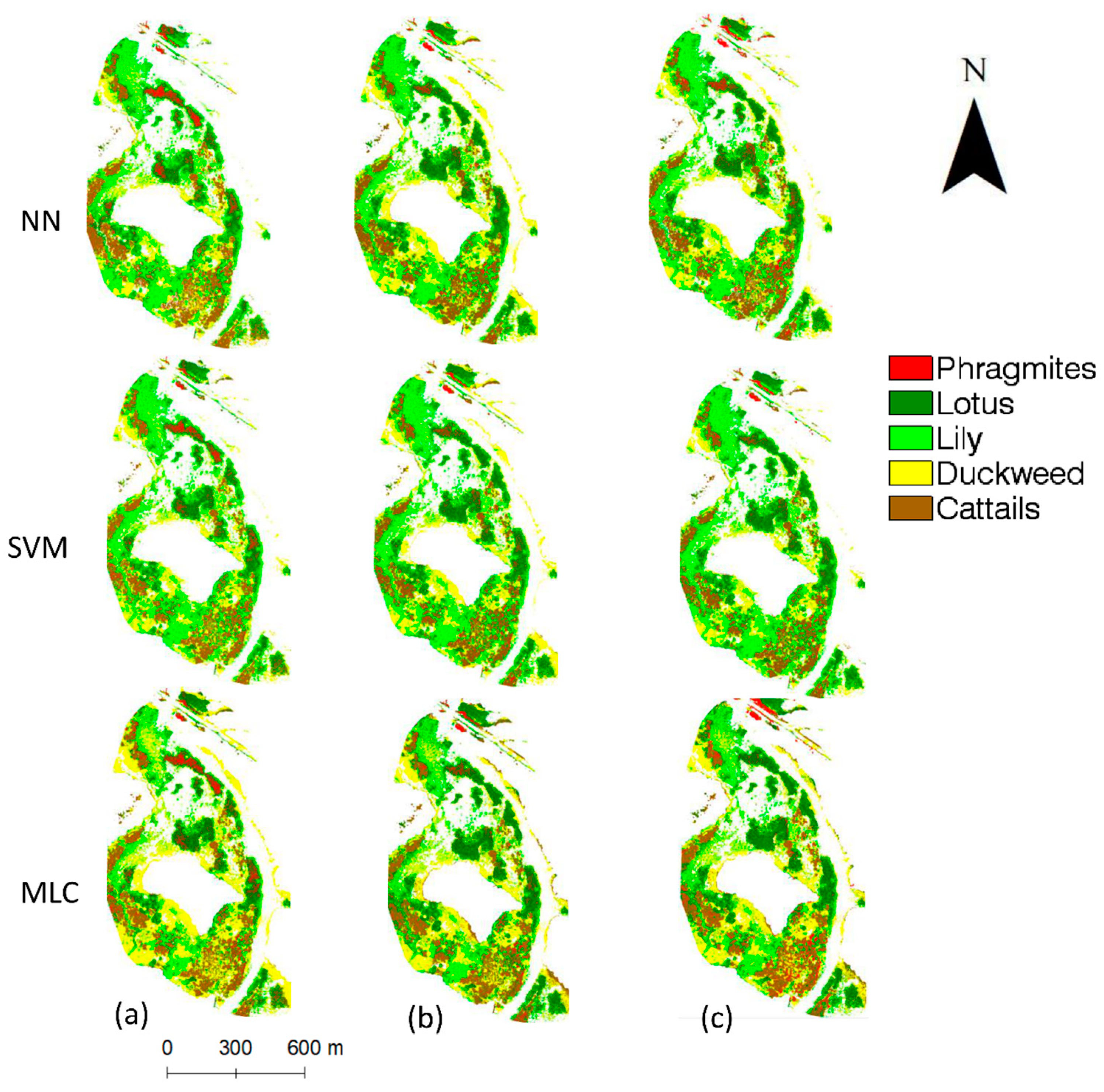
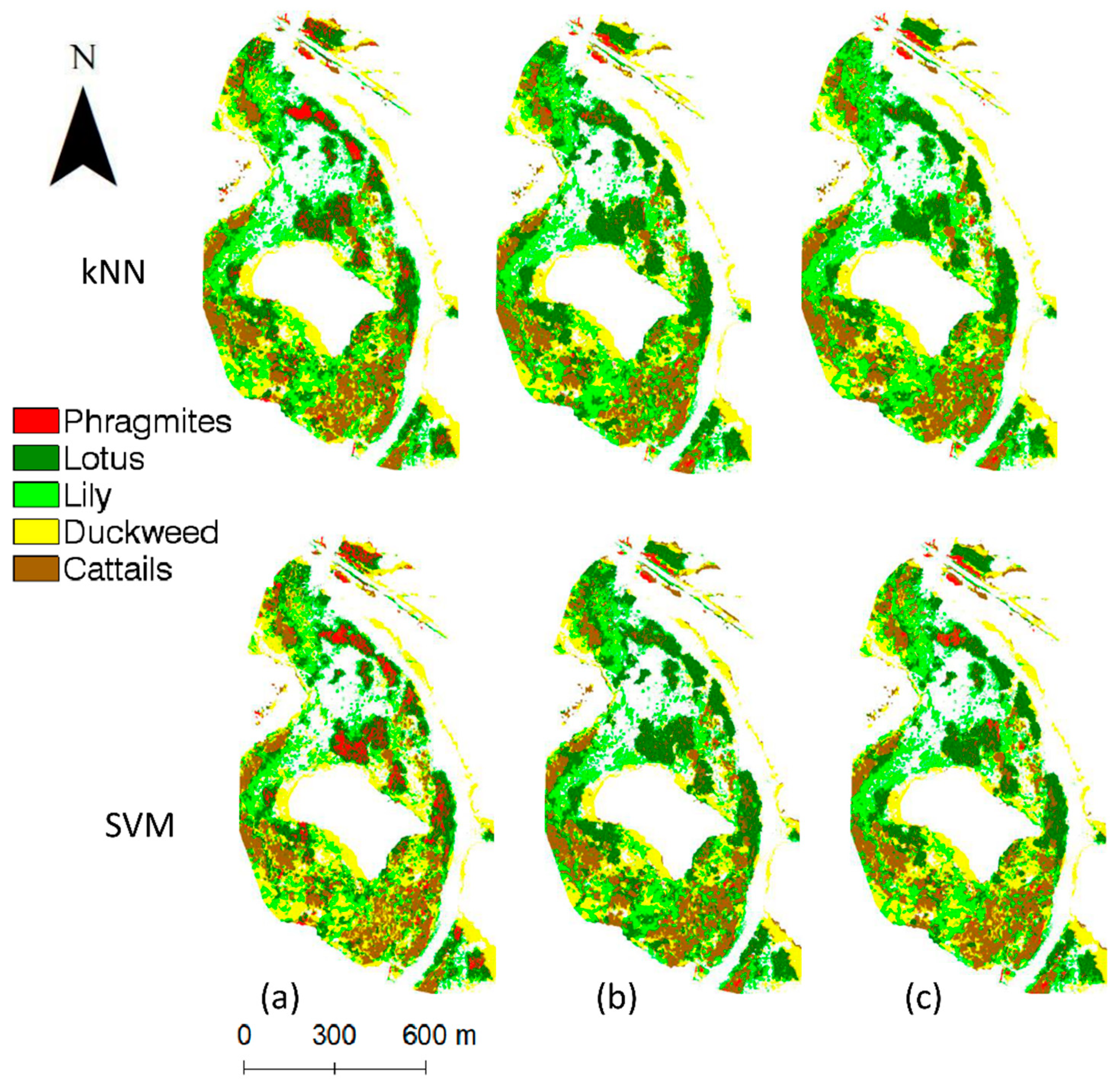
The overall findings in this study can also be supported by visualizing the classified UAV images (Figure 6). The NN classifier corresponds to the highest classification accuracy of Phragmites and lowest misclassification of Phragmites into cattails. Among the selected classifiers in Figure 6, the object-based SVM shows the lowest Phragmites classification accuracy due to the misclassification of Phragmites into the cattails class. Similar visual details can be observed between Phragmites and lotus across the study site.
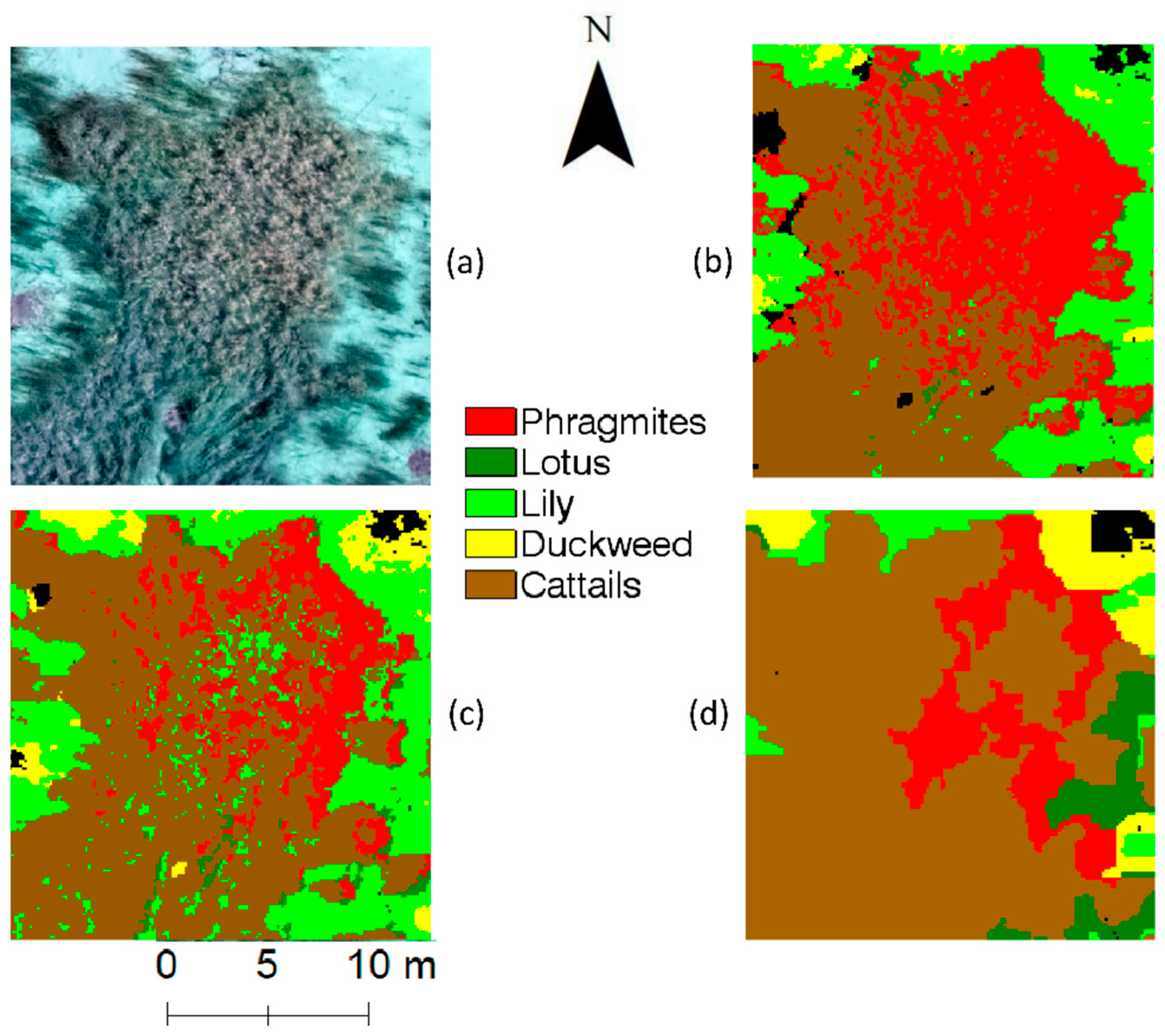
In comparison, between the pixel-based and object-based classifiers used in this study, there is a noticeable trend that the pixel-based NN classifier demonstrated the best results to detect Phragmites and the lowest error of omission (Figure 7). Furthermore, the findings suggest that there are no substantial differences between the ML classifiers and MLC in this study.

4. Discussion

This study demonstrates the advantage of using UAVs to map wetland species, especially to map small patches of invasive Phragmites in the OWC estuary, which would not be possible with coarse airborne and satellite images. This is well demonstrated by high OA for all sophisticated classifiers used in the study, and by relatively low errors of commission and omission for the given combination of feature layers.
Based on careful selection of ROIs, robust sampling design using cross-validation, and careful parameterization of the classifiers, the findings clearly demonstrate that the selection of feature layers is critical. It was clearly demonstrated that the combination of the raw images (4sq) with feature layers NDVIOct, and CHM, derived from UAV, produces the highest overall accuracy (OA = 94.80%) and the lowest error of omission (OE = 1.59%) as well as relatively low error of commission (CE = 4.51%) for Phragmites when NN is used. It was observed, during the field work, that Phragmites spread faster in the estuary than other plant types and to improve the eradication of Phragmites, the lowest omission error is a critical requirement. Phragmites can be effectively removed by mowing, burning, and applying herbicides during the summer or fall [77]. The low error of omission for Phragmites resulted in the study would provide an advantage for estuary management to reach and apply eradicating measures to almost all the Phragmites patches in the OWC estuary.

4.1. Feature Selection

The study demonstrates that too many features could decrease the classification accuracy, which agrees with the study of Price et al. [78]. The feature layers should be selected in such a way that they are most optimal in differentiating the classes [79], and this study has proposed to use NDVIOct and CHM to advance the classification of the UAV data. Although the main idea of the study was to concentrate on the August image, the integration of data acquired at different times, in late summer and in mid-fall, shows a clear advantage in this study [23]. A similar observation was reported by Lantz and Wang [80] and by several other studies where images at the end of the summer were successfully used to detect invasive Phragmites [33,81,82]. UAV data acquired in late spring (instead of late-growing season) might be equally useful. This would allow early detection and eradication of Phragmites and would help to overcome limitations observed in this study where the identification of hidden thin patches of Phragmites located under dense tree canopies was a challenge. Our efforts to collect UAV data over the study site in late spring were not successful due to frequent disturbances of the UAV flights by eagles nesting in the vicinity.
The importance of using CHM to identify Phragmites, as it reduces both errors of omission and commission, is also clearly demonstrated, especially when CHM is combined with NDVIOct. Several other studies showed the advantages of CHM [83,84,85]. The reduction of errors of omission and commission for Phragmites was observed in the study of Samiappan et al. [33], where the author used the SVM classifier. On the other hand, the use of textural and PC measurements does not show a considerable reduction of errors of omission and commission for Phragmites in this study, which was not the case in several studies [14,81,86] but was the case in the study of Bradly [22]. A similar trend was observed in both pixel- and object-based classification methods.

4.2. Sampling Design

A good sampling design is vital to achieve high classification accuracy [81]. A previous study [78] also highlighted that the complexity of the study site, characteristics of the remote sensing data, image pre-processing methods, and classification approach dictated the sampling design. As described by Stehman [87], an ideal sampling design should be cost-effective, providing meaningful results to achieve the classification objectives and accommodate any sampling data errors. However, it is not often practical to create a perfect sample design due to the limits of resources and field accessibility [87]. Foody et al. [75] studied possible methods to reduce the required training sample size without losing classification accuracy, suggesting that it was possible to use a small dataset when the mechanism of the classifier was known, and when the objective of the study was to map a specific class. However, selecting a sufficient number of training samples becomes a challenge in classification studies if the landscape consists of a smaller number of patches of a particular plant type or if the landscape is complex [78]. Based on all these principles, after lengthy exploration of various sampling approaches, the results in this study suggest that the stratified random sampling design is necessary for a wetland setup such as OWC. The reduction of the number of training and validation samples for Phragmites and duckweed classes is not expected to affect classification accuracies as the stratified random sampling design decreases any possible negative effect in this case.
Furthermore, Lucas et al. [88] claimed that a single pixel is the most suitable sample unit in a raster image for a pixel-based classification. However, if there are limitations such as poor accessibility, which was the case in this study, a sampling unit can consist of multiple pixels with an applied spatial smoothing technique as shown in this study [88]. A sample should include a sufficient number of basic classification sample units to represent all spectral properties of each class [69,77]. The grown ROIs include four or five pixels on average for each sampling point in this study covering higher spectral variability within each class. This approach increases the probability of classifying more pixels into the Phragmites class. In other words, the method can potentially reduce the errors of omission. The inclusion of more heterogeneous pixels in training and validation data is found to be promising to improve the classification accuracy [89]. The cross-validation method was applied to compensate for the relatively low, but still sufficient, number of samples per class in this study.

4.3. Object- vs. Pixel-Based Classification and Classification Algorithms

Several studies concluded that object-based classification performs better than pixel-based classification because it creates uniform objects by merging similar pixels into one object [37,72,90]. Specifically, Lantz and Wang [79] emphasized that the object-based classification method resulted in higher accuracy over pixel-based classification to identify invasive Phragmites, while Bradley [23] and Pande-Chhetri et al. [37] reported the opposite results when identifying some other invasive plants. Interestingly, the current study results in a higher error of omission for the object-based methods, similar to the study of Pande-Chhetri et al. [37]. Although the best scale parameter for segmentation was carefully selected in this study (as explained above), the segmentation could be slightly erroneous to the extent where Phragmites pixels are confused with the pixels of cattails due to similar pixel values. This confusion could lead Phragmites pixels to be aggregated in the segments that include cattails. This situation was observed during the process of segmentation in this study, especially at the boundaries between cattails and Phragmites. Therefore, the process of segmentation was an initial step where some uncertainties could be generated suggesting that this step is critical as small variability could lead to unexpected results. Edge enhancement techniques could be used to overcome such errors at the boundaries of segments and improve classification accuracy [91], which was not considered in this study.
Overall, no considerable advantages of ML classifiers over MLC are observed in this study. The similar overall accuracy, lower errors of commission, and the slightly higher errors of omission for MLC praise this parametric method as highly advanced. The findings show that the ML methods are not considerably better for the most optimal layer combination (4sq + NDVIOct + CHM), and that the tradeoffs between the ML classifiers and MLC should be considered given that the parameter optimization of SVM and NN classifiers need more time and effort compared to MLC. The disadvantage encountered with MLC in this study suggests that this classifier does not provide meaningful results when the number of bands increases to more than six. This was also demonstrated in the study of Cheeseman et al. [92]. In contrast, non-parametric classifiers (NN and SVM) are not considerably affected when the number of feature layers increases. High classification accuracies with the same classifiers were also achieved in the previous studies of Foody and Mathur [69], Ndehedehe et al. [65] and Qian et al. [68]. While some studies suggested that SVM outperformed NN in overall classification accuracy [66,89,93], the finding results in this study suggest that NN is exceptionally efficient when the minimum error of omission is required. Both high classification accuracy and the lowest error of omission for Phragmites are reached with a NN classifier restricted to one hidden layer [67]. Higher flexibility of the NN classifier due to the availability of a large number of different synaptic weights between each pair of nodes [62] has classified more pixels situated at the boundaries between Phragmites and cattail patches into the Phragmites, resulting in a lower error of omission.

5. Conclusions

High-resolution images acquired by UAVs are useful in mapping and evaluating wetland invasive plants because of image spatial resolution, ease of handling, and time and cost flexibility. This study used three pixel-based (NN, SVM, and traditional MLC) and two object-based (SVM and kNN) classifiers to detect Phragmites in the Old Woman Creek (OWC) Estuary in Ohio, USA. The UAV image acquired on 8 August 2017 was classified at three different levels of complexity using the proposed classifiers based on: (i) the four original bands (G, R, RE, NIR) (4sq); (ii) the sensitivity analysis where one feature layer at a time was added to 4sq, including information from the October image; and (iii) the combination of representative feature layers with the best performance added to 4sq.
It was clearly demonstrated that the combination of the raw images (4sq) with feature layers NDVIOct and CHM, derived from UAV, produced the highest overall accuracy (OA = 94.80%) and the lowest error of omission (OE = 1.59%) as well as a relatively low error of commission (CE = 4.51%) for Phragmites when NN is used. NN is recognized as the most effective approach in minimizing the error of omission. The findings suggest that the pixel-based classification was advantageous over the object-based approach to identify small patches of Phragmites as found in the OWC estuary.
The study also included a detailed analysis of the sampling design and the number and distribution of ROIs, suggesting that stratified random sampling design with multi-pixels as a sampling unit was the most appropriate method to map small Phragmites patches. It was suggested that the sampling method combined with the cross-validation statistical approach is critical for any of the classifiers used in the study. Temporal variability of NDVI in combination with CHM are the two most important feature layers to reach the best performance of any of the classifiers. Any additional information, such as image texture and PC, was found not to be useful in this study, having a negative or neutral impact when combined with other layers in the process of classification. The findings show that the ML methods are not considerably better than MLC for the most optimal layer combination (4sq + NDVIOct + CHM), and that the tradeoffs between the ML classifiers and MLC should be considered in future studies. The study provides a method to detect invasive Phragmites with high accuracy in a small area using a limited number of samples.

Author Contributions

T.A. collected and analyzed data, and wrote the paper. A.S.M. edited the paper and provided guidance and support throughout the research process. K.A. supported with research resources during the fieldwork. B.H. contributed with her ecological expertise in differentiating plant species. P.R. assisted in data collection and helped in image processing. A.G. and A.V.-O. provided important suggestions on research method and revising the original paper.

Funding

This research received funds from the BGSU Geology Foundation.

Acknowledgments

The support from the staff of the Old Woman Creek National Estuarine Research Reserve is gratefully acknowledged.

Conflicts of Interest

The authors declare no conflict of interest.

References

  1. Belluco, E.; Camuffo, M.; Ferrari, S.; Modenese, L.; Sonia, S.; Marani, A.; Marani, M. Mapping salt-marsh vegetation by multispectral and hyperspectral remote sensing. Remote Sens. Environ. 2006, 105, 54–67. [Google Scholar] [CrossRef]
  2. Zedler, J.B.; Kercher, S. Causes and consequences of invasive plants in wetlands: Opportunities, opportunists, and outcomes. CRC Crit. Rev. Plant Sci. 2004, 23, 431–452. [Google Scholar] [CrossRef]
  3. Callaway, R.M.; Aschehoug, E.T. Invasive plants versus their new and old neighbors: A mechanism for exotic invasion. Science 2000, 290, 521–523. [Google Scholar] [CrossRef] [PubMed]
  4. Book Review: Invasive Species in the Pacific Northwest; University of Washington Press: Washington, WA, USA, 2008; Available online: https://escholarship.org/uc/item/8v3513zj (accessed on 12 November 2018).
  5. Nonnative Invasive Plants of Pacific Coast Forests. Available online: https://www.fs.fed.us/pnw/pubs/pnw_gtr817.pdf (accessed on 19 August 2018).
  6. Vilà, M.; Espinar, J.L.; Hejda, M.; Hulme, P.E.; Jarošík, V.; Maron, J.L.; Pergl, J.; Schaffner, U.; Sun, Y.; Pyšek, P. Ecological impacts of invasive alien plants: A meta-analysis of their effects on species, communities and ecosystems. Ecol. Lett. 2011, 14, 702–708. [Google Scholar] [CrossRef] [PubMed]
  7. Richrdson, D.M.; Petr, P.; Rejmánek, M.; Barbour, M.G.; Panetta, F.D.; West, C.J. Naturalization and invasion of alien plants: Concepts and definitions. Divers. Distrib. 2000, 6, 93–107. [Google Scholar] [CrossRef]
  8. Blackburn, T.M.; Pyšek, P.; Bacher, S.; Carlton, J.T.; Duncan, R.P.; Jarošik, V.; Wilson, J.R.; Richardson, D.M. A proposed unified framework for biological invasions. Trends Ecol. Evol. 2011, 26, 333–339. [Google Scholar] [CrossRef] [Green Version]
  9. Sainty, G.; McCorkelle, G.; Julien, M. Control and spread of Alligator Weed Alternanthera philoxeroides (Mart.) Griseb., in Australia: Lessons for other regions. Wetl. Ecol. Manag. 1997, 5, 195–201. [Google Scholar] [CrossRef]
  10. Weidenhamer, J.D.; Callaway, R.M. Direct and indirect effects of invasive plants on soil chemistry and ecosystem function. J. Chem. Ecol. 2010, 36, 59–69. [Google Scholar] [CrossRef]
  11. Plant Guide for Common Reed (Phragmites australis). Available online: https://plants.usda.gov/plantguide/pdf/pg_phau7.pdf (accessed on 17 November 2018).
  12. Chambers, R.M.; Meyerson, L.A.; Saltonstall, K. Expansion of Phragmites australis into tidal wetlands of North America. Aquat. Bot. 1999, 64, 261–273. [Google Scholar] [CrossRef]
  13. Hudon, C.; Gagnon, P.; Jean, M. Hydrological factors controlling the spread of common reed (Phragmites australis) in theSt. Lawrence River (Québec, Canada). Ecoscience 2005, 12, 347–357. [Google Scholar] [CrossRef]
  14. Samiappan, S.; Turnage, G.; Hathcock, L.; Casagrande, L.; Stinson, P.; Moorhead, R. Using unmanned aerial vehicles for high-resolution remote sensing to map invasive Phragmites australis in coastal wetlands. Int. J. Remote Sens. 2017, 38, 2199–2217. [Google Scholar] [CrossRef]
  15. Mal, T.K.; Narine, L. The biology of Canadian weeds. 129. Phragmites australis (Cav.) Trin. ex Steud. Can. J. Palnt Sci. 2004, 84, 365–396. [Google Scholar]
  16. Mauchamp, A.; Blanch, S.; Grillas, P. Effects of submergence on the growth of Phragmites australis seedlings. Aquat. Bot. 2001, 69, 147–164. [Google Scholar] [CrossRef]
  17. Leonard, L.A.; Wren, P.A.; Beavers, R.L. Flow dynamics and sedimentation in Spartina alterniflora and Phragmites australis marshes of the Chesapeake Bay. Wetlands 2002, 22, 415–424. [Google Scholar] [CrossRef]
  18. Meyer, D.L.; Johnson, J.M.; Gill, J.W. Comparison of nekton use of Phragmites australis and Spartina alterniflora marshes in the Chesapeake Bay, USA. Mar. Ecol. Prog. Ser. 2001, 209, 71–83. [Google Scholar] [CrossRef]
  19. Lawrence, R.L.; Wood, S.D.; Sheley, R.L. Mapping invasive plants using hyperspectral imagery and Breiman Cutler classifications (RandomForest). Remote Sens. Environ. 2006, 100, 356–362. [Google Scholar] [CrossRef]
  20. Bustamante, J.; Aragonés, D.; Afán, I.; Luque, C.; Pérez-Vázquez, A.; Castellanos, E.; Díaz-Delgado, R. Hyperspectral sensors as a management tool to prevent the invasion of the cxotic cordgrass Spartina densiflora in the Doñana Wetlands. Remote Sens. 2016, 8, 1001. [Google Scholar] [CrossRef]
  21. Underwood, E.; Ustin, S.; DiPietro, D. Mapping nonnative plants using hyperspectral imagery. Remote Sens. Environ. 2003, 86, 150–161. [Google Scholar] [CrossRef]
  22. Müllerová, J.; Brůna, J.; Bartaloš, T.; Dvořák, P.; Vítková, M.; Pyšek, P. Timing is important: Unmanned aircraft vs. satellite imagery in plant invasion monitoring. Front. Plant Sci. 2017, 8, 887. [Google Scholar] [CrossRef]
  23. Bradley, B.A. Remote detection of invasive plants: A review of spectral, textural and phenological approaches. Biol. Invasions 2014, 16, 1411–1425. [Google Scholar] [CrossRef]
  24. Dronova, I. Object-based image analysis in wetland research: A review. Remote Sens. 2015, 7, 6380–6413. [Google Scholar] [CrossRef]
  25. Laliberte, A.S.; Herrick, J.E.; Rango, A.; Winters, C. Acquisition, orthorectification, and object-based classification of unmanned aerial vehicle (UAV) imagery for rangeland monitoring. Photogramm. Eng. Remote Sens. 2010, 76, 661–672. [Google Scholar] [CrossRef]
  26. Zhou, G.; Li, R. Accuracy evaluation of ground points from IKONOS high-resolution satellite imagery. Photogramm. Eng. Remote Sens. 2000, 66, 1103–1112. [Google Scholar]
  27. Ghioca-Robrecht, D.M.; Johnston, C.A.; Tulbure, M.G. Assessing the use of multiseason QuickBird imagery for mapping invasive species in a Lake Erie coastal marsh. Wetlands 2008, 28, 1028–1039. [Google Scholar] [CrossRef]
  28. Pengra, B.W.; Johnston, C.A.; Loveland, T.R. Mapping an invasive plant, Phragmites australis, in coastal wetlands using the EO-1 Hyperion hyperspectral sensor. Remote Sens. Environ. 2007, 108, 74–81. [Google Scholar] [CrossRef]
  29. Alvarez-Taboada, F.; Paredes, C.; Julián-Pelaz, J. Mapping of the invasive species Hakea sericea using unmanned aerial vehicle (UAV) and WorldView-2 imagery and an object-oriented approach. Remote Sens. 2017, 9, 913. [Google Scholar] [CrossRef]
  30. Lechner, A.M.; Fletcher, A.; Johansen, K.; Erskine, P. Characterising upland swamps using object-based classification methods and hyper-spatial resolution imagery derived from an unmanned aerial vehicle. In Proceedings of the XXII ISPRS Congress Annals of the Photogrammetry, Remote Sensing and Spatial Information Sciences, Melbourne, Australia, 25 August–1 September 2012; pp. 101–106. [Google Scholar]
  31. Tóth, V.R. Monitoring spatial variability and temporal dynamics of Phragmites using unmanned aerial vehicles. Front. Plant Sci. 2018, 9, 728. [Google Scholar] [CrossRef]
  32. Niphadkar, M.; Nagendra, H.; Tarantino, C.; Adamo, M.; Blonda, P. Comparing pixel and object-based approaches to map an understorey invasive shrub in tropical mixed forests. Front. Plant Sci. 2017, 8, 892. [Google Scholar] [CrossRef]
  33. Samiappan, S.; Turnage, G.; Hathcock, L.A.; Moorhead, R. Mapping of invasive phragmites (common reed) in Gulf of Mexico coastal wetlands using multispectral imagery and small unmanned aerial systems. Int. J. Remote Sens. 2017, 38, 2861–2882. [Google Scholar] [CrossRef]
  34. Thomas, Z.; Turney, C.; Palmer, J.; Lloydd, S.; Klaricich, J.; Hogg, A. Extending the observational record to provide new insights into invasive alien species in a coastal dune environment of New Zealand. Appl. Geogr. 2018, 98, 100–109. [Google Scholar] [CrossRef]
  35. Berni, J.A.; Zarco-Tejada, P.J.; Suárez, L.; Fereres, E. Thermal and narrowband multispectral remote sensing for vegetation monitoring from an unmanned aerial vehicle. IEEE Trans. Geosci. Remote Sens. 2009, 47, 722–738. [Google Scholar] [CrossRef]
  36. Komárek, J.; Klouček, T.; Prošek, J. The potential of unmanned aerial systems: A tool towards precision classification of hard-to-distinguish vegetation types? Int. J. Appl. Earth Obs. Geoinf. 2018, 71, 9–19. [Google Scholar] [CrossRef]
  37. Pande-Chhetri, R.; Abd-Elrahman, A.; Liu, T.; Morton, J.; Wilhelm, V.L. Object-based classification of wetland vegetation using very high-resolution unmanned air system imagery. Eur. J. Remote Sens. 2017, 50, 564–576. [Google Scholar] [CrossRef] [Green Version]
  38. Puliti, S.; Ørka, H.; Gobakken, T.; Næsset, E. Inventory of small forest areas using an unmanned aerial system. Remote Sens. 2015, 7, 9632–9654. [Google Scholar] [CrossRef]
  39. Tang, L.; Shao, G. Drone remote sensing for forestry research and practices. J. For. Res. 2015, 26, 791–797. [Google Scholar] [CrossRef]
  40. Zhang, J. Multi-source remote sensing data fusion: Status and trends. Int. J. Image Data Fusion 2010, 1, 5–24. [Google Scholar] [CrossRef]
  41. Lisein, J.; Pierrot-Deseilligny, M.; Bonnet, S.; Lejeune, P. A photogrammetric workflow for the creation of a forest canopy height model from small unmanned aerial system imagery. Forests 2013, 4, 922–944. [Google Scholar] [CrossRef]
  42. Klarer, D.M.; Millie, D.F. Aquatic macrophytes and algae at Old Woman Creek estuary and other Great Lakes coastal wetlands. J. Great Lakes Res. 1992, 18, 622–633. [Google Scholar] [CrossRef]
  43. Whyte, R.S.; Trexel-Kroll, D.; Klarer, D.M.; Shields, R.; Francko, D.A. The invasion and spread of Phragmites australis during a period of low water in a Lake Erie coastal wetland. J. Coast. Res. 2008, 111–120. [Google Scholar] [CrossRef]
  44. Herdendorf, C.E.; Klarer, D.M.; Herdendorf, R.C. Ecology. In The Ecology of Old Woman Creek: An Estuarine and Watershed Profile; Ohio Department of Natural Resources, Division of Natural Areas and Preserves: Columbus, OH, USA, 2006; p. 1. [Google Scholar]
  45. ArcGIS base Maps. Esri, DigitalGlobe, GeoEye, Earthstar Geographics, CNES/Airbus DS, USDA, USGS, AeroGRID, IGN, HERE, Garmin, © OpenStreetMap Contributors, and the GIS User Community. Available online: https://www.arcgis.com/home/group.html?id=702026e41f6641fb85da88efe79dc166#overview (accessed on 2 February 2019).
  46. Lopez, F.; Klarer, D.; Elmer, H.; Keefe, A.; Zoest, P.V.; Pasterak, G. Estuaries: Critical National Resources. In Old Woman Creek National Estuarine Research Reserve Management Plan 2011–2016; Ohio Department of Natural Resources, Division of Wildlife: Huron, OH, USA, 2011. [Google Scholar]
  47. Aday, D.D. The Presence of and invasive macrophyte (Phragmites australis) Does not Influence Juvenile Fish Habitat Use in a Freshwater Estuary. J. Freshw. Ecol. 2007, 22, 535–537. [Google Scholar] [CrossRef]
  48. eBee SQ The Advanced Agriculture Drone. Available online: https://www.sensefly.com/drone/ebee-sq-agriculture-drone/ (accessed on 9 June 2017).
  49. eMotion. Available online: https://www.sensefly.com/software/emotion/ (accessed on 13 June 2017).
  50. Full Range/High Resolution Field Portable Spectroradiometers for Remote Sensing. Available online: https://spectralevolution.com/products/hardware/field-portable-spectroradiometers-for-remote-sensing/ (accessed on 10 May 2017).
  51. Pix4Dmapper. Available online: https://www.pix4d.com/product/pix4dmapper-photogrammetry-software (accessed on 23 May 2017).
  52. Gamon, J.A.; Field, C.B.; Goulden, M.L.; Griffin, K.L.; Hartley, A.E.; Joel, G.; Penuelas, J.; Valentini, R. Relationships between NDVI, canopy structure, and photosynthesis in three Californian vegetation types. Ecol. Appl. 1995, 5, 28–41. [Google Scholar] [CrossRef]
  53. Barnes, E.; Clarke, T.; Richards, S.; Colaizzi, P.; Haberland, J.; Kostrzewski, M.; Waller, P.; Choi, C.; Riley, E.; Thompson, T. Coincident detection of crop water stress, nitrogen status and canopy density using ground based multispectral data. In Proceedings of the Fifth International Conference on Precision Agriculture, Bloomington, MN, USA, 16–19 July 2000. [Google Scholar]
  54. Han, Y.; Li, M.; Li, D. Vegetation index analysis of multi-source remote sensing data in coal mine wasteland. N. Z. J. Agric. Res. 2007, 50, 1243–1248. [Google Scholar] [CrossRef]
  55. Jordan, C.F. Derivation of leaf-area index from quality of light on the forest floor. Ecology 1969, 50, 663–666. [Google Scholar] [CrossRef]
  56. Buschmann, C.; Nagel, E. In vivo spectroscopy and internal optics of leaves as basis for remote sensing of vegetation. Int. J. Remote Sens. 1993, 14, 711–722. [Google Scholar] [CrossRef]
  57. Xue, J.; Su, B. Significant remote sensing vegetation indices: A review of developments and applications. J. Sens. 2017, 2017, 1–17. [Google Scholar] [CrossRef]
  58. Gitelson, A.A.; Merzlyak, M.N. Signature analysis of leaf reflectance spectra: Algorithm development for remote sensing of chlorophyll. J. Plant Physiol. 1996, 148, 494–500. [Google Scholar] [CrossRef]
  59. Chavez, P.S., Jr. Comparison of spatial variability in visible and near-infrared spectral images. Photogramm. Eng. Remote Sens. 1992, 58, 957–964. [Google Scholar]
  60. Principal Components Analysis. Available online: https://www.harrisgeospatial.com/docs/PrincipalComponentAnalysis.html (accessed on 25 March 2018).
  61. Yunfei, B.; Guoping, L.; Chunxiang, C.; Xiaowen, L.; Zhang, H.; Qisheng, H.; Linyan, B.; Chaoyi, C. Classification of lidar point cloud and generation of dtm from lidar height and intensity data in forested area. Int. Arch. Photogramm. Remote Sens. Spat. Inf. Sci. 2008, 37, 313–318. [Google Scholar]
  62. eCognition Developer 9. Available online: http://www.ecognition.com/suite/ecognition-developer (accessed on 9 November 2017).
  63. eCognition User Community. Available online: http://community.ecognition.com/home/when-you-have-landsat-data-do-not-perform-radiometric-calibration-toa.-is-it-true/view?searchterm=multiply+100#1440684094 (accessed on 25 February 2018).
  64. Maxwell, A.E.; Warner, T.A.; Fang, F. Implementation of machine-learning classification in remote sensing: An applied review. Int. J. Remote Sens. 2018, 39, 2784–2817. [Google Scholar] [CrossRef]
  65. Ndehedehe, C.; Ekpa, A.; Simeon, O.; Nse, O. Understanding the neural network technique for classification of remote sensing data sets. N. Y. Sci. J. 2013, 6, 26–33. [Google Scholar]
  66. Mas, J.F.; Flores, J.J. The application of artificial neural networks to the analysis of remotely sensed data. Int. J. Remote Sens. 2008, 29, 617–663. [Google Scholar] [CrossRef]
  67. Duro, D.C.; Franklin, S.E.; Dubé, M.G. A comparison of pixel-based and object-based image analysis with selected machine learning algorithms for the classification of agricultural landscapes using SPOT-5 HRG imagery. Remote Sens. Environ. 2012, 118, 259–272. [Google Scholar] [CrossRef]
  68. Qian, Y.; Zhou, W.; Yan, J.; Li, W.; Han, L. Comparing machine learning classifiers for object-based land cover classification using very high resolution imagery. Remote Sens. 2015, 7, 153–168. [Google Scholar] [CrossRef]
  69. Foody, G.M.; Mathur, A. Toward intelligent training of supervised image classifications: Directing training data acquisition for SVM classification. Remote Sens. Environ. 2004, 93, 107–117. [Google Scholar] [CrossRef]
  70. Mountrakis, G.; Im, J.; Ogole, C. Support vector machines in remote sensing: A review. ISPRS J. Photogramm. Remote Sens. 2011, 66, 247–259. [Google Scholar] [CrossRef]
  71. Rupasinghe, P.A.; Simic Milas, A.; Arend, K.; Simonson, M.A.; Mayer, C.; Mackey, S. Classification of shoreline vegetation in the Western Basin of Lake Erie using airborne hyperspectral imager HSI2, Pleiades and UAV data. Int. J. Remote Sens. 2018, 40, 3008–3028. [Google Scholar] [CrossRef]
  72. Whiteside, T.G.; Boggs, G.S.; Maier, S.W. Comparing object-based and pixel-based classifications for mapping savannas. Int. J. Appl. Earth Obs. Geoinf. 2011, 13, 884–893. [Google Scholar] [CrossRef]
  73. Stehman, S.V.; Czaplewski, R.L. Design and analysis for thematic map accuracy assessment: Fundamental principles. Remote Sens. Environ. 1998, 64, 331–344. [Google Scholar] [CrossRef]
  74. Region of Interest (ROI) Tool. Available online: https://www.harrisgeospatial.com/docs/RegionOfInterest Tool.html (accessed on 18 February 2018).
  75. Foody, G.M.; Mathur, A.; Sanchez-Hernandez, C.; Boyd, D.S. Training set size requirements for the classification of a specific class. Remote Sens. Environ. 2006, 104, 1–14. [Google Scholar] [CrossRef]
  76. Kotsiantis, S.B.; Zaharakis, I.; Pintelas, P. Supervised machine learning: A review of classification techniques. Informatica 2007, 2007, 249–268. [Google Scholar]
  77. Güsewell, S. Management of Phragmites australis in swiss fen meadows by mowing in early summer. Wetl. Ecol. Manag. 2003, 11, 433–445. [Google Scholar] [CrossRef]
  78. Price, K.P.; Guo, X.; Stiles, J.M. Optimal Landsat TM band combinations and vegetation indices for discrimination of six grassland types in eastern Kansas. Int. J. Remote Sens. 2002, 23, 5031–5042. [Google Scholar] [CrossRef]
  79. Lu, D.; Weng, Q. A survey of image classification methods and techniques for improving classification performance. Int. J. Remote Sens. 2007, 28, 823–870. [Google Scholar] [CrossRef]
  80. Lantz, N.J.; Wang, J. Object-based classification of Worldview-2 imagery for mapping invasive common reed, Phragmites australis. Can. J. Remote Sens. 2013, 39, 328–340. [Google Scholar] [CrossRef]
  81. Laba, M.; Blair, B.; Downs, R.; Monger, B.; Philpot, W.; Smith, S.; Sullivan, P.; Baveye, P.C. Use of textural measurements to map invasive wetland plants in the Hudson River National Estuarine Research Reserve with IKONOS satellite imagery. Remote Sens. Environ. 2010, 114, 876–886. [Google Scholar] [CrossRef]
  82. Gilmore, M.S.; Wilson, E.H.; Barrett, N.; Civco, D.L.; Prisloe, S.; Hurd, J.D.; Chadwick, C. Integrating multi-temporal spectral and structural information to map wetland vegetation in a lower Connecticut River tidal marsh. Remote Sens. Environ. 2008, 112, 4048–4060. [Google Scholar] [CrossRef]
  83. de Castro, A.; Torres-Sánchez, J.; Peña, J.; Jiménez-Brenes, F.; Csillik, O.; López-Granados, F. An automatic random forest-OBIA algorithm for early weed mapping between and within crop rows using UAV imagery. Remote Sens. 2018, 10, 285. [Google Scholar] [CrossRef]
  84. Martin, F.-M.; Müllerová, J.; Borgniet, L.; Dommanget, F.; Breton, V.; Evette, A. Using single-and multi-date UAV and satellite imagery to accurately monitor invasive knotweed species. Remote Sens. 2018, 10, 1662. [Google Scholar] [CrossRef]
  85. Sankey, T.; Donager, J.; McVay, J.; Sankey, J.B. UAV lidar and hyperspectral fusion for forest monitoring in the southwestern USA. Remote Sens. Environ. 2017, 195, 30–43. [Google Scholar] [CrossRef]
  86. Liu, J. A Combined Method for Vegetation Classification Based on Visible Bands from UAV Images: A Case Study for Invasive Wild Parsnip Plants. Master’s Thesis, Queen’s University, Kingston, ON, Canada, February 2018. [Google Scholar]
  87. Stehman, S.V. Sampling designs for accuracy assessment of land cover. Int. J. Remote Sens. 2009, 30, 5243–5272. [Google Scholar] [CrossRef]
  88. Lucas, I.; Janssen, F.; van der Wel, F.J. Accuracy assessment of satellite derived landcover data: A review. Photogramm. Eng. Remote Sens. 1994, 60, 419–426. [Google Scholar]
  89. Shao, Y.; Lunetta, R.S. Comparison of support vector machine, neural network, and CART algorithms for the land-cover classification using limited training data points. ISPRS J. Photogramm. Remote Sens. 2012, 70, 78–87. [Google Scholar] [CrossRef]
  90. Yu, Q.; Gong, P.; Clinton, N.; Biging, G.; Kelly, M.; Schirokauer, D. Object-based detailed vegetation classification with airborne high spatial resolution remote sensing imagery. Photogramm. Eng. Remote Sens. 2006, 72, 799–811. [Google Scholar] [CrossRef]
  91. Ali, M.; Clausi, D. Using the Canny edge detector for feature extraction and enhancement of remote sensing images. In Proceedings of the IEEE 2001 International Geoscience and Remote Sensing Symposium, Waterloo, ON, Canada, 9–13 July 2001; pp. 2298–2300. [Google Scholar]
  92. Cheeseman, P.C.; Self, M.; Kelly, J.; Taylor, W.; Freeman, D.; Stutz, J.C. Bayesian Classification. In Proceedings of the AAAI, Moffett Field, CA, USA, 21 August 1988; pp. 607–611. [Google Scholar]
  93. Omer, G.; Mutanga, O.; Abdel-Rahman, E.M.; Adam, E. Performance of support vector machines and artificial neural network for mapping endangered tree species using WorldView-2 data in Dukuduku forest, South Africa. IEEE J. Sel. Top. Appl. Earth. Obs. Remote. Sens. 2015, 8, 4825–4840. [Google Scholar] [CrossRef]
Figure 1. Study area located on the southern shoreline of Lake Erie, Ohio, USA [45].
Remotesensing 11 01380 g001
Figure 2. Workflow of the study.
Remotesensing 11 01380 g002
Figure 3. Unmanned aerial vehicle (UAV) images using (a) Sequoia camera on 8 August 2017; (b) Sequoia on 18 October 2017 (false colors near-infrared (NIR) band in red, red band in green, red edge (RE) band in blue in both images); and (c) RGB camera taken on 8 August 2017 (true color image).
Remotesensing 11 01380 g003
Figure 4. Averaged spectral signatures of the plants of interest in the Old Woman Creek (OWC) estuary. The color bars show the spectral ranges of green (G), red (R), red edge (RE) and near-infrared (NIR) bands of the Sequoia camera.
Remotesensing 11 01380 g004
Figure 5. Mapping wetland vegetation in OWC using pixel-based neural network (NN) support vector machine (SVM), and maximum likelihood classifier (MLC) classifiers for (a) 4Sq, (b) 4sq+NDVIOct, (c) 4Sq+NDVIOct+canopy height model (CHM).
Remotesensing 11 01380 g005
Figure 6. Mapping wetland vegetation in OWC using the object-based SVM and k-nearest neighbor (kNN) classifiers for (a) 4sq, (b) 4sq+NDVIOct, (c) 4sq+NDVIOct +CHM.
Remotesensing 11 01380 g006
Figure 7. (a) Phragmites patch (grayish in the middle) observed in the RGB image (for the purpose of validation); (b) pixel-based NN classified image; (c) pixel-based SVM classified image; (d) object-based SVM classified image. Note: all classified images are based on the most optimal 4sq+NDVIOct+CHM combination.
Remotesensing 11 01380 g007
Table 1. Normalized and simple band indices used in the classification methods.
Band IndexEquationReference
NDVI(NIR—Red)/(NIR + Red)[52]
NDRE(NIR—Red Edge)/(NIR + Red Edge)[53]
NDGI(NIR—Green)/(NIR + Green)[54]
SR1NIR/Red[55]
SR2NIR/Green[56]
SR3NIR/Red Edge[57]
SR4Red Edge/Red[58]
SR5Red/Green[57]
SR6Green/Red Edge[58]
NDVI = Normalized Difference Vegetation Index; NIR = Near-Infrared; NDRE = Normalized Difference Red Edge; NDGI = Normalized Difference Green Index; SR = Simple Ratio.
Table 2. Parametrization using four original bands for pixel- and object-based classification methods.
TypeClassifierParameterValue
Pixel-basedSVMC50
Gamma0.25
NNTTC0.20
TR0.20
TM0.90
RMSEC0.01
NHL1
NI1000
Object-basedSVMC100
Gamma0.001
kNNk2
TTC = Training threshold contribution; TR = Training rate; TM = Training momentum; RMSEC = Root mean square exit criteria; NHL = Number of hidden layers; NI = Number of iterations.
Table 3. Accuracy assessment for each class of the 4sq image. Misclassification among Phragmites, cattails, and lotus, and overall classification accuracy and kappa values for each classifier (CE = errors of commission; OE = errors of omission).
ClassClass Accuracy %CE %OE %
Phragmites82.4215.6817.58
Cattails98.282.701.72
Lotus82.3516.9517.65
Lily90.518.909.49
Duckweed97.834.642.17
ClassCommission (Phragmites) %Omission (Phragmites) %
Cattails1.151.59
Lotus8.8915.99
ClassifierOA %Kappa
NN84.580.81
SVM90.470.88
MLC88.230.85
Table 4. Results of ANOVAs performed among Normalized Difference Vegetation Index (NDVI) values of Phragmites, cattails, and lotus generated for the 8 August and 18 October images.
DateANOVA Test
Ap-ValueMean NDVI Value
8 August0.050.26Phragmites (0.76), Cattails (0.77), Lotus (0.81)
18 October0.050.00Phragmites (0.45), Cattails (0.23), Lotus (0.12)
Tukey Kramer Test (Absolute Difference / Critical Range)
18 OctoberPhragmites vs. Cattails 34.39/5.84
Phragmites vs. Lotus 14.78/5.84
Cattails vs. Lotus 19.61/5.84
Table 5. Overall accuracy (OA), kappa value, errors of commission (CE) and omission (OE) for Phragmites class (Ph) for the case when each layer is separately stacked to 4sq (pixel-based classification using support vector machine (SVM)).
Feature TypeLayerOA %KappaCE % (Ph)OE % (Ph)
Band Indices (8 October)NIR/Green92.290.904.0020.69
NIR/Red90.970.8913.8519.79
NDVI93.430.924.865.56
NDGI91.140.899.8020.69
NDRE92.570.918.1622.41
NIR/Red Edge91.710.905.8817.24
Red Edge/Red90.860.898.0020.69
Green/Red Edge90.860.898.1622.41
Red/Green90.220.8815.6218.37
Texture (8 August)Mean91.140.8910.2024.14
Variance91.710.907.6917.24
Homogeneity93.140.912.0818.97
Contrast90.570.888.1622.41
Dissimilarity93.140.912.0817.97
Entropy91.710.902.1320.69
Second moment92.280.902.0818.97
Correlation92.570.919.8020.69
Elevation (August 8)CHM93.590.921.759.53
Principal Components (August 8)PC191.140.890.0015.52
PC293.710.9216.0618.97
PC390.000.8715.0922.41
PC490.280.888.1622.41
Table 6. Overall accuracy (OA) and kappa value, Phragmites class classification accuracy, and errors of commission (CE) and omission (OE) for pixel-based classification methods with feature layers stacked to 4sq image.
Classifier4sq4sq+NDVIOct4sq+NDVIOct+CHM4sq+NDVIOct+CHM+PC14sq+NDVIOct+CHM+PC1+Var
OA%KappaOA%KappaOA%KappaOA%KappaOA%Kappa
NN84.580.8191.260.8994.800.9392.960.9194.680.93
SVM90.470.8893.430.9294.580.9394.330.9393.120.91
MLC88.230.8593.460.9292.920.91N.A.N.A.N.A.N.A.
Phragmites Class Classification Accuracy %
NN82.3096.0398.4196.0397.58
SVM82.4294.4395.2494.4594.45
MLC87.2695.2496.83N.A.N.A.
CE %OE %CE %OE %CE %OE %CE %OE %CE %OE %
NN22.5317.706.063.974.511.593.133.972.962.42
SVM15.6817.584.865.563.036.763.035.553.035.55
MLC20.5812.743.624.762.223.17N.A.N.A.N.A.N.A.
Table 7. Overall accuracy (OA) and kappa value, Phragmites class classification accuracy, and errors of commission (CE) and omission (OE) for object-based classification methods with feature layers stacked to 4sq image.
Classifier4sq4sq+NDVIOct4sq+NDVIOct+CHM4sq+NDVIOct+CHM + PC14sq+NDVIOct+CHM+PC1+Var
OA%KappaOA%KappaOA%KappaOA%KappaOA%Kappa
SVM87.690.8489.230.8692.310.9092.300.9091.540.89
kNN86.920.8484.620.8189.230.8690.770.8884.620.81
Phragmites Class Classification Accuracy %
SVM75.0080.7092.5892.3090.45
kNN75.3060.3591.0089.2589.10
ClassifierCE %OE %CE %OE %CE %OE %CE %OE %CE %OE %
SVM28.5725.0010.2015.403.575.323.956.255.756.38
kNN2.1320.691.5040.001.7810.201.5010.431.2510.35

