Adaptive Contrast Enhancement for Infrared Images Based on the Neighborhood Conditional Histogram

Abstract

In this paper, an adaptive contrast enhancement method based on the neighborhood conditional histogram is proposed to improve the visual quality of thermal infrared images. Existing block-based local contrast enhancement methods usually suffer from the over-enhancement of smooth regions or the loss of some details. To address these drawbacks, we first introduce a neighborhood conditional histogram to adaptively enhance the contrast and avoid the over-enhancement caused by the original histogram. Then the clip-redistributed histogram of the contrast-limited adaptive histogram equalization (CLAHE) is replaced by the neighborhood conditional histogram. In addition, the local mapping function of each sub-block is updated based on the global mapping function to further eliminate the block artifacts. Lastly, the optimized local contrast enhancement process, which combines both global and local enhanced results is employed to obtain the desired enhanced result. Experiments are conducted to evaluate the performance of the proposed method and the other five methods are introduced as a comparison. Qualitative and quantitative evaluation results demonstrate that the proposed method outperforms the other block-based methods on local contrast enhancement, visual quality improvement, and noise suppression.

1. Introduction

With the ability to convert the passively received infrared radiation into infrared images, infrared imaging systems have been widely used in military and civilian fields, for instance, thermal remote sensing, weapon guidance, night vision, fire detection, and disease diagnosis [1,2,3,4,5]. In these fields, infrared imaging has superiority and application prospects that are incomparable to visual imaging. However, compared with visual images, the raw infrared images usually suffer from poor contrast and low resolution, which are the main factors that limit the performance of infrared imaging systems [6]. Therefore, contrast enhancement is one of the indispensable pre-processing methods in infrared imaging systems to improve the visual quality of infrared images [7].

Contrast enhancement methods for infrared images have been studied for decades, and most of them are based on the most famous and classical method histogram equalization (HE) [8]. According to the scope of the mapping function of the contrast enhancement method, these methods can be classified into two categories: global contrast enhancement (GCE) and local contrast enhancement (LCE) [9]. In the GCE methods, one global mapping function which corresponds to the entire image characteristics is applied to each pixel of the image. On the contrary, in LCE methods, multiple local mapping functions are used to enhance the contrast of their corresponding areas of the image.

Among the GCE methods, HE is the most well-known one and has been widely applied due to its low computational complexity and effectiveness. In HE, the contrast enhancement ratio of each grayscale is proportional to its probability distribution function. Therefore, the enhanced result may appear over-enhancement in the homogeneous regions, especially when the homogeneous regions account for a large proportion in the infrared images [10]. To address this drawback, there are many improved HE methods investigated. The plateau histogram equalization (PHE) [11,12], double plateaus histogram equalization (DPHE) [13], and adaptive double plateaus histogram equalization (ADPHE) [14] attempt to limit the contrast by introducing one or two proper thresholds to avoid over-enhancement. Other methods, such as the brightness preserving bi-histogram equalization (BBHE) [15], dualistic sub-image histogram equalization (DSIHE) [16], recursive mean-separate histogram equalization (RMSHE) [17], adaptive histogram segmentation (AHS) [7], and adaptive histogram partition (AHP) [18], adaptively divide the histogram into two or more intervals, then carry out histogram equalization in each interval within the assigned grayscale range. Additionally, the histogram modification framework (HMF) [19] and histogram specification (HS) [20] are also effective methods to avoid the over-enhancement of HE. The GCE methods generally enhance the contrast based on the entire image characteristics with low computational complexity and favorable light order preservation. However, the global mapping function is not suitable for various regions with different local contrast characteristics, which is the limitation of GCE methods.

To improve the performance of GCE methods, the LCE methods are developed to enhance the local contrast based on the characteristics of local regions. The two representative methods of them are the contrast limited adaptively histogram equalization (CLAHE) [21] and partially overlapped sub-block histogram equalization (POSHE) [22]. In CLAHE, the input image is divided into multiple non-overlapped sub-blocks. In each sub-block, the histogram is clipped and redistributed to avoid over-enhancement. In addition, to avoid the appearance of block artifacts, bilinear interpolation is carried out between mapping functions of the adjacent sub-blocks. In POSHE, the input image is divided into multiple partially overlapped sub-blocks. Histogram equalization is carried out in each sub-block, for the pixels in overlapped regions, the enhanced results are the average value of correlated sub-blocks. As an improvement of CLAHE, the balanced CLAHE and contrast enhancement (BCCE) [23] improves the redistribution mechanism and introduces an exponential factor to enhance the local contrast. Nevertheless, the block artifacts and noise amplification may still appear in the large homogeneous regions of the enhanced results. Therefore, the adjacent-blocks-based modification for local histogram equalization (ABMHE) [24] and local gradient-grayscale statistical feature (LGGSF) [25] take the content of each sub-block into consideration when calculating the corresponding mapping function. In ABMHE, the partially overlapped sub-blocks are categorized into three categories based on the gradient information. Not only the category of each sub-block but also that of its adjacent sub-blocks are taken into consideration when calculating the mapping function. In LGGSF, the non-overlapped sub-blocks are categorized into two categories using the classification model trained by a support vector machine (SVM). The mapping function of each sub-block is calculated according to its category. These classification-based LCE methods get better performance on eliminating the block artifacts. However, the improper classification in the transition regions or the low contrast regions may result in the loss of detail. In addition to the block-based methods, the adaptive trilateral contrast enhancement (ATCE) [26] manipulates the contrast, sharpness, and intensity based on the modified histogram and the extracted feature of the input image. Other models, such as the unsharp masking [27,28], retinex theory [29], and wavelet transform [30,31,32], can also be utilized to improve the visual quality of infrared images. These LCE methods produce better local contrast enhanced result than GCE methods, however, they may still suffer from noise amplification, block artifacts, and/or loss of details.

In our previous paper [33], we tried to improve the visual quality of infrared images by combining the merits of both GCE and LCE methods. In that paper, the global and local histogram specification (GLHS) enhances the contrast of infrared images by applying histogram specification globally and locally based on the 2D histogram of the input image. Then the local contrast is enhanced based on both global and local enhancement results. Whereas the utilization of 2D histogram makes GLHS a time-consuming method, we found the global–local conception can be utilized to improve the CLAHE method. Therefore, in this paper, an adaptive contrast enhancement method based on the neighborhood conditional histogram is proposed to improve the visual quality of infrared images. First, the neighborhood conditional histogram is proposed to avoid the over-enhancement caused by the original histogram. When extracting the neighborhood conditional histogram of the input image, the neighbor content of each pixel is taken into consideration. In this way, the gray levels of the pixels located in the detail regions will get a high probability distribution function and will, accordingly, get a high contrast enhancement ratio, and vice versa, if the pixels are located in homogeneous regions. Then, for the improvement of CLAHE, we replace the clip-redistributed histogram with the proposed neighborhood conditional histogram. And to eliminate the block artifacts, the mapping function of each sub-block is updated based on the global mapping function. Lastly, the local contrast is optimized and enhanced based on both global and local enhanced result. The remainder of this paper is organized as follows. In Section 2, we first review and discuss the CLAHE. In Section 3, the proposed method is described in detail. In Section 4, experiments are conducted, and the analysis of the experimental results are given. In Section 5, the conclusion is drawn.

2. Review of CLAHE

CLAHE is an extension of the adaptive histogram equalization (AHE) algorithm [34]. These two methods are dedicated to solving the over-enhancement problem of HE. Over-enhancement is caused by the inherent drawback of HE. For a given infrared image $X$ with $L$ gray levels, the histogram can be expressed as

$$H(l)=n_l,l=0,1,\cdots ,L-1,$$

(1)

where $n_l$ indicates the number of pixels with a gray level $l$ in the image. Based on the definition of HE and assuming that the dynamic range of the enhanced result is $R$(256 for the 8-bit images), the enhanced result of the gray level $l$ is calculated by

$$y_l=T(l)=\frac{R-1}{N}{\displaystyle {\sum }_{k=0}^{l}H(k)},$$

(2)

where $T(l)$ is the mapping function and maps the gray level $l$ of the input image into $y_l$ of the output image, $N$ is the total number of pixels in $X$. Therefore, for the enhanced image, the contrast enhancement ratio of the adjacent gray levels in the input image is

$${\delta }_l=y_l-y_{l-1}=\frac{R-1}{N}\cdot H(l).$$

(3)

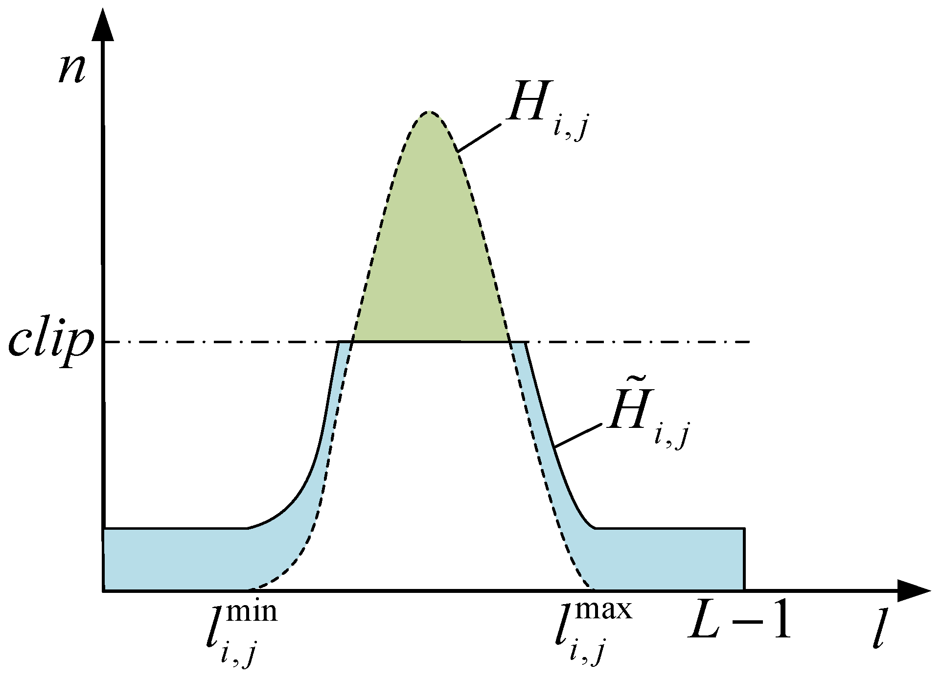
As can be seen in Equation (3), the value of ${\delta }_l$ is proportional to the corresponding histogram value. Which means, for the HE method, the gray level with a high histogram value also has a high enhancement ratio and occupies most grayscale range [7]. Unfortunately, the gray levels with histogram values usually belong to the pixels in the background or large homogeneous area. For these gray levels, high enhancement ratios and grayscale ranges result in unnaturalness and wash-out appearance, and the noise in the homogeneous regions will be amplified. At the same time, the other gray levels belonging to the pixels in the detail area cannot get desired enhancement ratios and grayscale ranges. This is the reason why HE usually causes over-enhancement for infrared images. In CLAHE, to avoid the over-enhancement of the homogeneous regions and get better contrast enhancement in detail regions, the image is divided into a grid of rectangular contextual sub-blocks [21], in each sub-block, HE is carried out. For each sub-block, $H_{i,j}$ is used to represent the histogram of the sub-block $(i,j)$. To avoid over-enhancement, $H_{i,j}$ is adjusted by clipping and redistribution [35] to get ${\tilde{H}}_{i,j}$. The mechanism of this adjustment is shown in Figure 1. Where $l_{i,j}^{\min }$ and $l_{i,j}^{\max }$ are the minimum and maximum gray levels within the sub-block, respectively. The pixels in the green area of $H_{i,j}$ are redistributed to the blue area, thus ${\tilde{H}}_{i,j}$ is consists of the blue area and the part of $H_{i,j}$ below clip limit intuitively. This adjustment process is implemented by iteration [35].

As can be seen from the previous discussion, it is obvious that the enhancement ratio is related to the value of the clip limit. That is, a higher value of the clip limit results in more contrast enhancement of the corresponding gray levels. The clip limit of the original CLAHE method is a pre-defined value [21,36] and is invariant to the image content

$$clip=\frac{N_b}{L}+\alpha (N_b-\frac{N_b}{L}),$$

(4)

where $N_b$ is the number of pixels in each sub-block, $\alpha$ is the clip factor within range $[0,1]$. Based on Equation (4), the range of clip limit is $\left[N_b/L,N_b\right]$. When the clip limit is equal to $N_b/L$, the redistributed histogram ${\tilde{H}}_{i,j}$ turns to be a uniformly distributed histogram ${\tilde{H}}_{i,j}(l)=N_b/L$, which linearly maps the input image of range $\left[0,L-1\right]$ to the output image of range $\left[0,R-1\right]$. Whereas, if the clip limit is higher than the histogram peak, the redistributed histogram ${\tilde{H}}_{i,j}$ is equal to the original histogram $H_{i,j}$. It can also be observed that the clip limit determined by Equation (4) is the same for each sub-block. Based on ${\tilde{H}}_{i,j}$, the mapping function of each sub-block is computed by

$$T_{i,j}(l)=\frac{R-1}{N_b}\cdot {\displaystyle {\sum }_{k=0}^l{\tilde{H}}_{i,j}(k)},l=0,1,\cdots ,L-1,$$

(5)

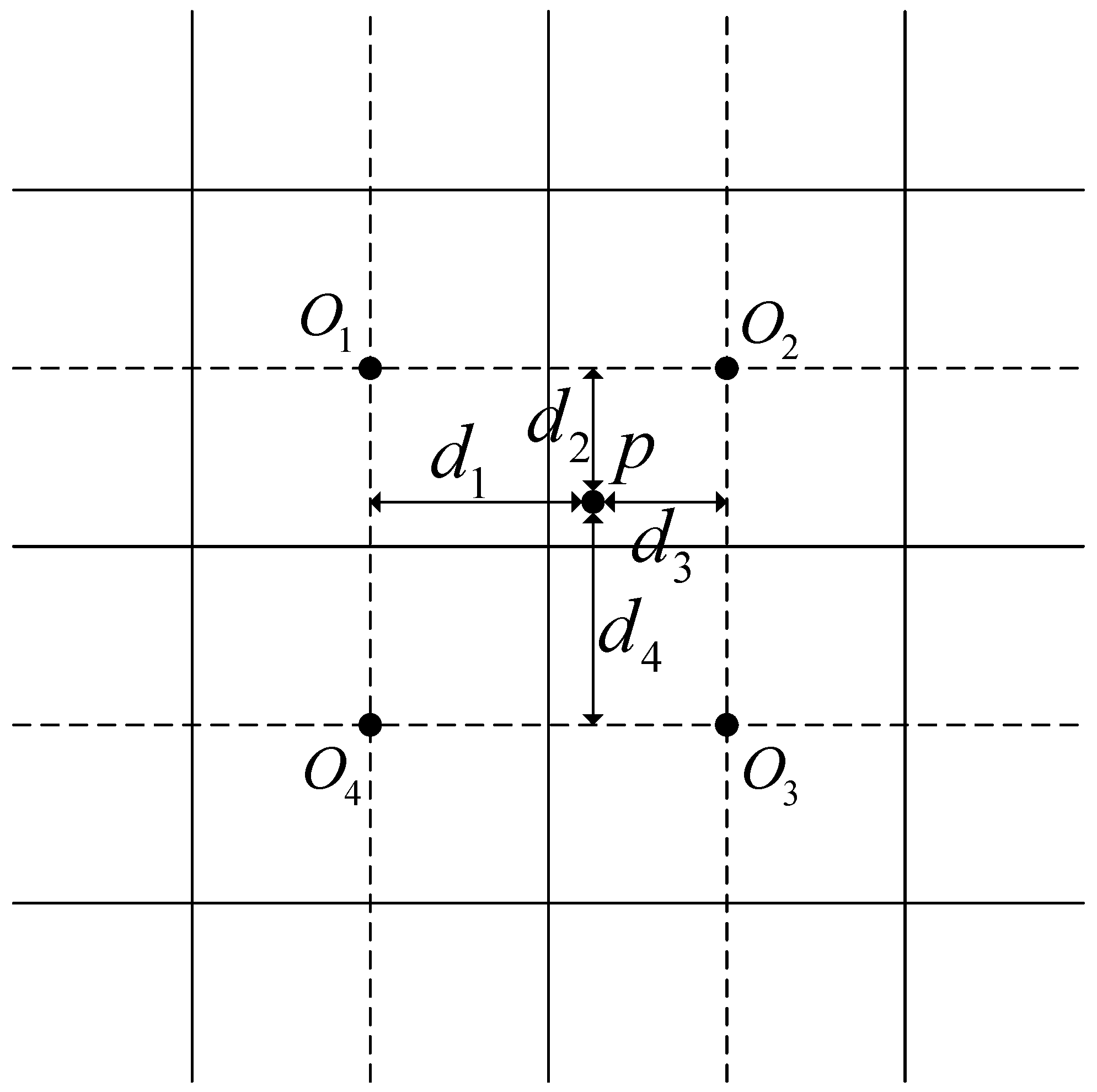
where $T_{i,j}(l)$ is the mapping function of the sub-block $(i,j)$. Due to the calculation of mapping functions being independent of each other, the block artifacts are inevitable. Therefore, to prevent the block artifacts, the mapping result of each pixel should take the mapping functions of the nearest four sub-blocks into consideration. For an arbitrary pixel $p$, the final remapped result is computed based on the bilinear interpolation [21] and is expressed as:

$$T(X_p)=\frac{d_3{d}_4{T}_1(X_p)+d_1{d}_4{T}_2(X_p)+d_1{d}_2{T}_3(X_p)+d_2{d}_3{T}_4(X_p)}{(d_1+d_3)(d_2+d_4)},$$

(6)

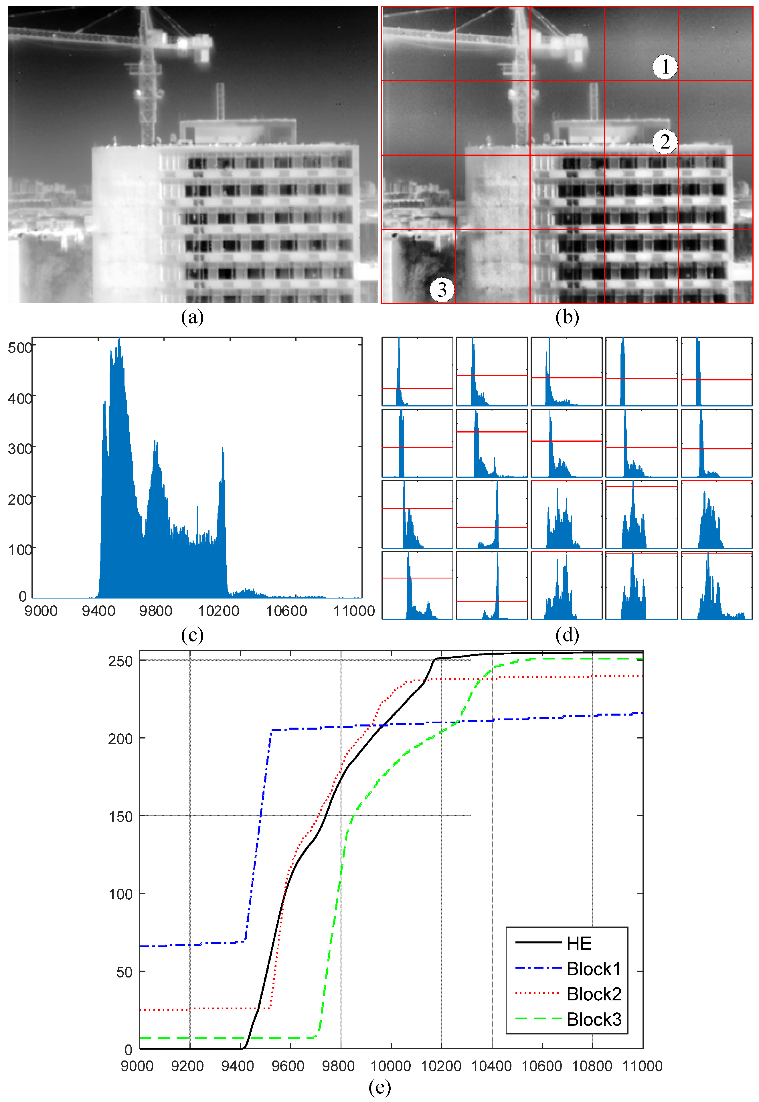
where $X_p$ is the gray value of the pixel $p$ in the input image, $T$ is an intermediate variable, $T_1(\cdot )$, $T_2(\cdot )$, $T_3(\cdot )$, and $T_4(\cdot )$ are the mapping functions of the corresponding sub-blocks centered on $O_1$, $O_2$, $O_3$, and $O_4$ as shown in Figure 2. Take an infrared image as an example, the HE result and CLAHE result of the given image are given in Figure 3. Here the resolution of the given image is $320\times 256$, and the size of each sub-block is $64\times 64$. The clip limit of CLAHE is computed by Equation (4), and we set $\alpha =0.01$ for the given image.

As shown in Figure 3, the contrast of the detail regions is not well enhanced in the HE result, and the CLAHE performs much better on contrast enhancement in these regions. However, in the homogeneous regions, the noise is over-enhancement and artifacts emerge in the CLAHE result. As discussed before, for the HE result, the contrast enhancement ratio of each gray level in the input image is proportional to the corresponding histogram value. Thus for the CLAHE, the maximum contrast enhancement ratio of each sub-block is determined by the clip limit. The clip limit is computed based on Equation (4) and is unrelated to the content of each sub-block. As a matter of fact, a higher clip limit is required for the sub-blocks with texture and details to get effective contrast enhancement. On the contrary, the sub-blocks with concentrated gray level distribution need a relatively lower clip limit to avoid the enhancement of noise. It is obvious that a constant clip limit is not suitable for CLAHE. In [37], the researchers introduced a mechanism to adaptively set the clip limit based on the content of each sub-block. This mechanism works for the 8-bit visual images, but it is not applicable to the captured 14-bit infrared images due to its being useless in the noise suppression of homogeneous regions. In addition to the noise amplification, the block artifacts are not completely eliminated in the homogeneous regions, as shown in Figure 3b. This is caused by the very different mapping results when applying the nearest four mapping function to the same gray levels if there are different proportions of homogeneous regions in the sub-blocks. Hence, the block artifacts still exist in the bilinear interpolation results.

3. Proposed Method

To avoid over-enhancement of homogeneous regions and effectively enhance the contrast of detail-rich regions, we replace the clip-redistributed histogram with our proposed neighborhood conditional histogram. In our proposed neighborhood conditional histogram, the image content is taken into consideration when computing the histogram. Therefore, the corresponding mapping function of each sub-block is able to automatically adapt to the content of each sub-block. Then, for the further elimination of block artifacts, the local mapping functions are updated based on the global mapping function. Lastly, the optimized local contrast enhanced result is obtained by making an optimization between the local Weber contrast of global and local enhanced results. In the following part, our proposed method is described in detail.

3.1. Neighborhood Conditional Histogram

As discussed in the previous section, the contrast enhancement ratio of each gray level after HE is proportional to the corresponding histogram value. In HE, for the pixels in homogeneous regions, the corresponding gray levels tend to get higher histogram values than other gray levels. Thus, this usually leads to the over-enhancement in the homogeneous regions and lack-enhancement in the detail regions. To address this problem, we try to take the image content into consideration when performing the histogram statistic. In our proposed neighborhood conditional histogram, the gray levels located in detail regions get higher histogram values than those located in homogeneous regions. The neighborhood conditional histogram of $X$ is expressed as

$$H(l)={\displaystyle \sum _{a=1}^A{\displaystyle \sum _{b=1}^B\left[\frac{1}{w_r-1}{\displaystyle \sum _{i=-r}^r{\displaystyle \sum _{j=-r}^r{\varphi }_l(X_{a,b},X_{a+i,b+j},t)}}\right]}},$$

(7)

where $A\times B$ represents the size of the given image, $r$ is an integer introduced to determine the radius of the square neighborhood around each pixel, $w_r={(2r+1)}^2$ is the number of pixels in the square neighborhood, $t$ is a predefined threshold, ${\varphi }_l(u,v,t)$ is defined to be a binary function and is expressed as follows:

$${\varphi }_l(u,v,t)=\{\begin{array}{cc}1& ifu=land\left|u-v\right|\ge t\\ 0& otherwise\end{array}.$$

(8)

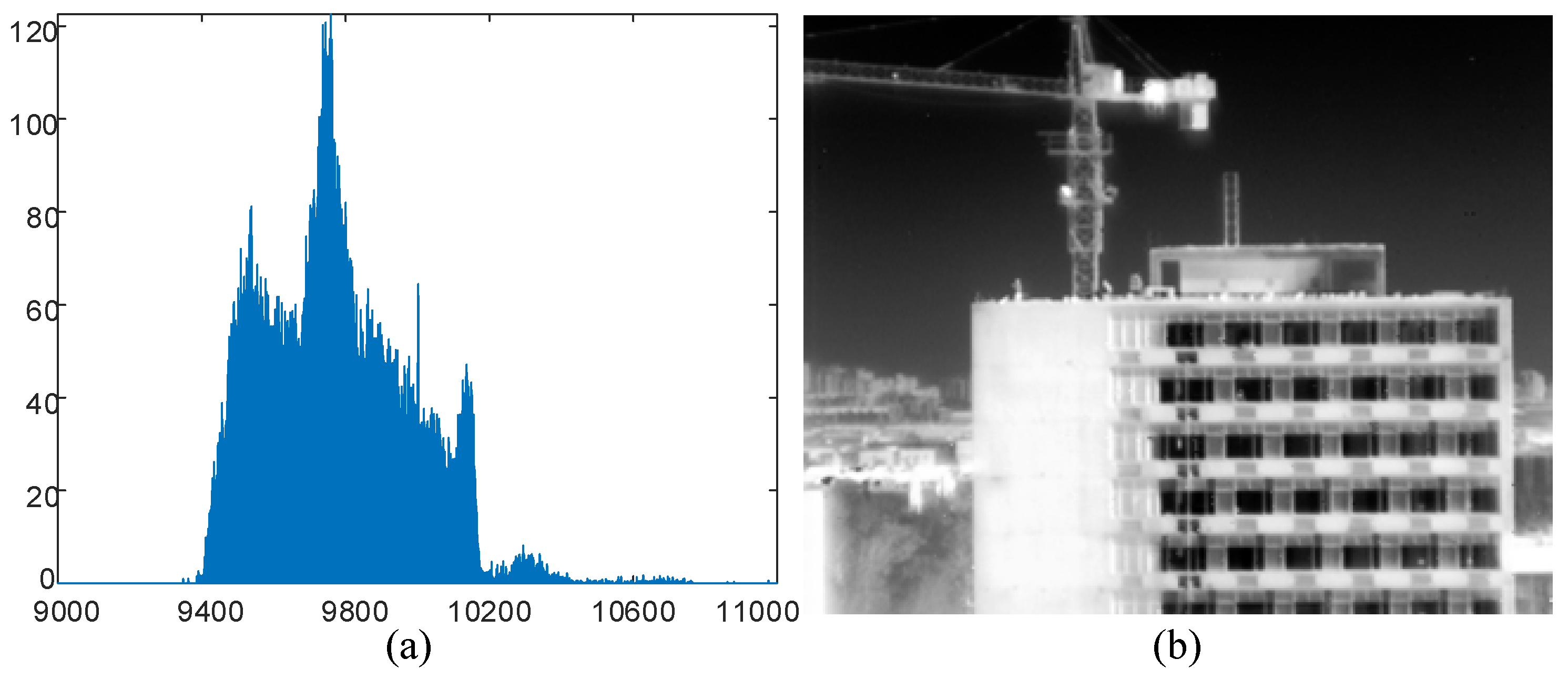
By defining the binary function for each pixel and its neighbors, the image content is able to be taken into consideration when computing the histogram value. Thus, a higher value of any gray level in our proposed neighborhood conditional histogram does not mean that the gray level has a larger probability of occurrence in the image. Instead, a higher value represents that the pixels that take on the corresponding gray level have a larger probability of being located in the detail regions. For the gray levels with a higher histogram value a better contrast enhancement after HE can be achieved. Hence, our proposed neighborhood conditional histogram is more reasonable than the original histogram. Based on Equation (2), the mapping function of the neighborhood conditional histogram can be obtained. The enhanced result of the given infrared image based on our proposed neighborhood conditional histogram is given in Figure 4. The parameters are set as $r=2$ and $t=10$ here for the given 14-bit infrared image. It is obvious that the neighborhood conditional histogram in Figure 4a looks much different from the histogram in Figure 3c. And the enhanced result looks much better than the original HE result.

3.2. Improved CLAHE

As discussed in the previous sub-section, our proposed neighborhood conditional histogram outperforms the original histogram on adaptively enhancing the contrast of infrared images. Therefore, for the improvement of CLAHE, we propose to replace the clip-redistributed histogram with the neighborhood conditional histogram. By applying the neighborhood conditional histogram to each sub-block, the new histogram of sub-block $(i,j)$ is obtained and denoted as $H_{i,j}^{\ast }$. And then the corresponding local mapping function $T_{i,j}^{\ast }(l)$ is computed by replacing ${\tilde{H}}_{i,j}(k)$ in Equation (5) with $H_{i,j}^{\ast }(k)$. Obviously, if the mapping function $T_{i,j}^{\ast }(l)$ is applied to the sub-block $(i,j)$, the artifacts will still appear in the homogeneous regions after the bilinear interpolation. With this consideration, the local mapping functions have to be updated. As for the sub-blocks of the given infrared image, an indisputable fact is that each sub-block is just a part of the whole image. Thus, not only the mapping function of each sub-block but also the global mapping function have to be taken into consideration to update the local mapping functions. The local mapping functions are calculated based on the image content of the corresponding sub-blocks. Due to the calculation processes of the local mapping functions being carried out independently, the contrast of each sub-block can be well enhanced. However, the block artifacts may appear in the final enhanced result. On the contrary, the global mapping function is computed based on the whole image content. Therefore, there are no artifacts in the enhanced result, but the local contrast enhancement is not as good as the enhanced result using the local mapping functions. Considering the complementary characteristics of the global mapping function and the local mapping functions, we update the local mapping functions by making an adaptive compromise between the local mapping function and the global mapping function.

The global mapping function $T_G^{\ast }(l)$ is obtained by substituting $H_G^{\ast }(l)$ into Equation (2). Here $H_G^{\ast }(l)$ represents the neighborhood conditional histogram of the whole infrared image and is computed by adding the neighborhood conditional histograms of the sub-blocks together.

$$H_G^{\ast }(l)={\displaystyle \sum _i{\displaystyle \sum _j{H}_{i,j}^{\ast }(l)}}.$$

(9)

The updated local mapping function ${\tilde{T}}_{i,j}^{\ast }$ is treated as the solution to a bi-criteria optimization problem [33]. We use the squared of the Euclidean norm for optimization. Hence, the updated mapping function is computed by

$${\tilde{T}}_{i,j}^{\ast }=\underset{T}{\arg \min }{\Vert T-T_G^{\ast }\Vert }_2^2+ƛ{\Vert T-T_{i,j}^{\ast }\Vert }_2^2,$$

(10)

where $T$ is an intermediate variable, $ƛ$ is a regularization parameter and varies over $\left[0,\infty \right)$. The solution to this quadratic optimization problem is

$${\tilde{T}}_{i,j}^{\ast }=(1-\beta )T_G^{\ast }+\beta T_{i,j}^{\ast },$$

(11)

where

$$\beta =\frac{ƛ}{1+ƛ}.$$

As $ƛ$ varies over $\left[0,\infty \right)$, the value of $\beta$ is within the range of $\left[0,1\right]$. It is obvious that the updated local mapping function ${\tilde{T}}_{i,j}^{\ast }$ turns out to be a weighted average of $T_G^{\ast }$ and $T_{i,j}^{\ast }$. By varying $\beta$, the weights of $T_G^{\ast }$ and $T_{i,j}^{\ast }$ in ${\tilde{T}}_{i,j}^{\ast }$ change accordingly. When $\beta =0$, ${\tilde{T}}_{i,j}^{\ast }$ is equal to the global mapping function $T_G^{\ast }$. Thus the enhanced result of sub-block $(i,j)$ using ${\tilde{T}}_{i,j}^{\ast }$ is the same as the global enhanced result using $T_G^{\ast }$. As $\beta$ increases and approaches $1$, ${\tilde{T}}_{i,j}^{\ast }$ gradually converges to the original local mapping function $T_{i,j}^{\ast }$ and the corresponding enhanced result of sub-block $(i,j)$ turns to resemble the enhanced result using $T_{i,j}^{\ast }$. Therefore, $\beta$ should be set as a block adaptive variable that has a different value depending on the block characteristics. This means it should be represented as the component of the sub-block ordered set $({\beta }_{i,j}\in \mathit{\beta })$ instead of the constant $\beta$. Considering this notation, the solution in Equation (11) is rewritten as

$${\tilde{T}}_{i,j}^{\ast }=(1-{\beta }_{i,j})T_G^{\ast }+{\beta }_{i,j}{T}_{i,j}^{\ast }.$$

(12)

As ${\beta }_{i,j}$ in Equation (12) is recommended to be a block adaptive value, it should be determined based on the block content. For the sub-blocks with a large proportion of homogeneous regions, a small ${\beta }_{i,j}$ is required to avoid the over-enhancement and the appearance of block artifacts. Whereas, a large ${\beta }_{i,j}$ is more suitable for the sub-blocks that contain many details and textures to get better contrast enhancement. When determining the value of ${\beta }_{i,j}$, it is reasonable to utilize the neighborhood conditional histogram $H_{i,j}^{\ast }$, which is also calculated based on the content of the sub-block $(i,j)$. Therefore, in our proposed method, ${\beta }_{i,j}$ is determined by

$${\beta }_{i,j}=\frac{{\displaystyle \sum _{l=0}^{L-1}{H}_{i,j}^{\ast }(l)}}{N_b}.$$

(13)

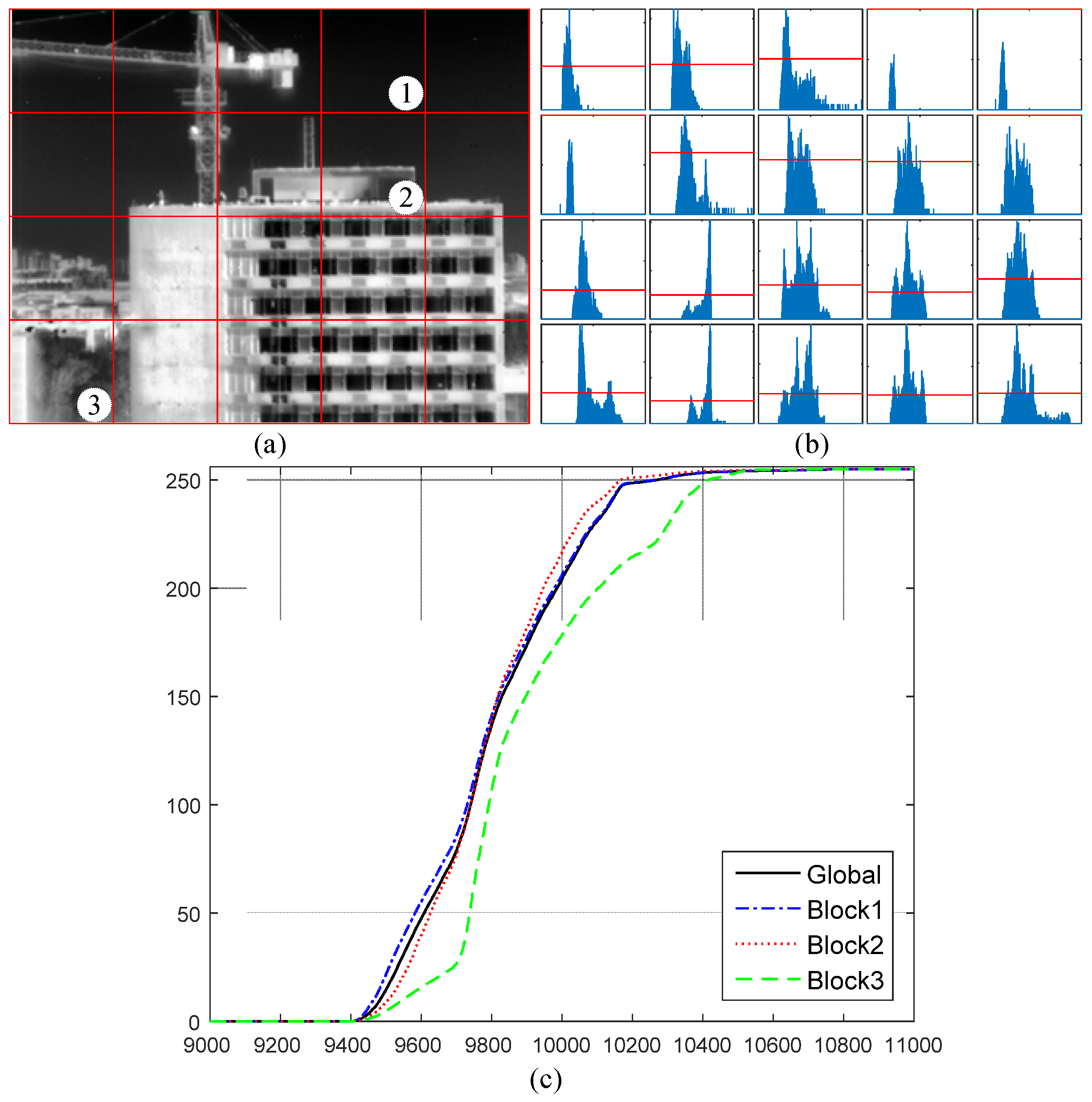
From the definition of $H_{i,j}^{\ast }$ in Equation (7), for the sub-block $(i,j)$, a higher value of $H_{i,j}^{\ast }$ indicates that there are more pixels with gray level $l$ located in the detail regions. This means that the sum of $H_{i,j}^{\ast }$ is larger if there are more details in the sub-block $(i,j)$, and accordingly, the value of ${\beta }_{i,j}$ is also larger as required. On the contrary, the value of ${\beta }_{i,j}$ for the sub-block with more homogeneous regions is also smaller. This is reflected in Figure 5, where it is clear that the homogeneous area accounts for a large proportion in sub-block 1 and sub-block 2. Therefore, the corresponding mapping functions resemble the global mapping function. As shown in Figure 5a, there are no artifacts in the homogeneous regions. This indicates that the improved CLAHE performs well on enhancing the local contrast with no artifacts.

3.3. Optimized Local Contrast Enhancement

To further enhance the local contrast and make the details more visible to human viewers, the optimized enhanced result is obtained by combining the local contrast of both global and local enhanced results. The global enhanced result $Y_G$ is computed by transferring the gray levels of the input infrared image to the output gray levels using the global mapping function $T_G^{\ast }$. The local enhanced result $Y_L$ is obtained by the improved CLAHE described in the previous sub-section. With reference to a given pixel of the desired enhanced result $Y$, the local Weber contrast is defined as

$$C_k=\frac{Y_k-{\overline{Y}}_k}{{\overline{Y}}_k},$$

(14)

where $C_k$ denotes the Weber contrast of the pixel $k$, ${\overline{Y}}_k$ represents the average gray intensity in the neighborhood of pixel $k$ and is computed by

$${\overline{Y}}_k=\frac{1}{\left|D_k\right|}{\displaystyle \sum _{i\in D_k}{Y}_i},$$

(15)

where $D_k$ represents the neighborhood of the pixel $k$ and $\left|D_k\right|$ is the total number of pixels in the neighborhood. To enhance the local contrast, we suppose that the estimated local contrast of $Y$ is expressed as

$${\tilde{C}}_k=c\times C_k^{\ast },$$

(16)

where ${\tilde{C}}_k$ is the estimated local contrast, $c$ is defined as the contrast parameter, $C_k^{\ast }$ is the baseline local contrast. Taking the local contrast of both global and local enhanced results into consideration, the baseline local contrast $C_k^{\ast }$ is computed by solving a bi-criteria optimization problem as follows:

$$C_k^{\ast }=\underset{C}{\arg \min }{\Vert C-C_{Gk}\Vert }^2+\lambda {\Vert C-C_{Lk}\Vert }^2,$$

(17)

where $C$ is an intermediate variable, $\lambda$ is defined as a regularization parameter and varies over $\left[0,\infty \right)$, $C_{Gk}$, and $C_{Lk}$, representing the local contrast of the global and local enhanced results, respectively, are calculated by $C_{Gk}=(Y_{Gk}-{\overline{Y}}_{Gk})/{\overline{Y}}_{Gk}$ and $C_{Lk}=(Y_{Lk}-{\overline{Y}}_{Lk})/{\overline{Y}}_{Lk}$. The optimal solution of Equation (17) is expressed as

$$C_k^{\ast }=\frac{1}{1+\lambda }{C}_{Gk}+\frac{\lambda }{1+\lambda }{C}_{Lk}.$$

(18)

As $\lambda$ varies from $0$ to $\infty$, the solution of $C_k^{\ast }$ in Equation (18) traces the optimal trade-off local contrast between $C_{Gk}$ and $C_{Lk}$. The baseline local contrast obtained by $\lambda =0$ corresponds to the contrast of global enhanced result, whereas when $\lambda$ increases to infinity, it resembles the contrast of the local enhanced result. Thus, we obtain different baseline local contrast according to $\lambda$. Taking the region characteristics of the input image into consideration, it is more reasonable to set $\lambda$ as a region adaptive variable instead of a constant value. This means $\lambda$ should be set as the component of the lexicographically ordered image (${\lambda }_k\in \mathit{\lambda }$). In the case of the contrast parameter $c$ in Equation (16), the enhancement level of the estimated local contrast ${\tilde{C}}_k$ is adjusted by the value of $c$. To adaptively enhance the local contrast, in the proposed method, $c$ is also determined to be a region adaptive variable by considering the regional characteristics. Therefore, the contrast parameter $c$ should also be set as the component of the lexicographically ordered image ($c_k\in \mathit{c}$) instead of a constant. Considering these notations and substituting Equation (18) into Equation (16), the estimated local contrast ${\tilde{C}}_k$ is rewritten as

$${\tilde{C}}_k=c_k(\frac{1}{1+{\lambda }_k}{C}_{Gk}+\frac{{\lambda }_k}{1+{\lambda }_k}{C}_{Lk}).$$

(19)

Combining Equations (14) and (19), the desired enhanced result $Y_k$ meets the formula below

$$\frac{Y_k-{\overline{Y}}_k}{{\overline{Y}}_k}=c_k(\frac{1}{1+{\lambda }_k}\cdot \frac{Y_{Gk}-{\overline{Y}}_{Gk}}{{\overline{Y}}_{Gk}}+\frac{{\lambda }_k}{1+{\lambda }_k}\cdot \frac{Y_{Lk}-{\overline{Y}}_{Lk}}{{\overline{Y}}_{Lk}}),$$

(20)

where ${\overline{Y}}_k$ indicated the average gray intensity of the pixel $k$ in the desired enhanced result, but the value is not given. To compute the desired enhanced result based on Equation (20), we assume that there is no significant difference between the average gray intensity of the local enhanced result and that of the desired enhanced result (${\overline{Y}}_k\approx {\overline{Y}}_{Lk}$). Then, the desired enhanced result $Y_k$ is computed by

$$Y_k={\overline{Y}}_{Lk}+c_k(\frac{1}{1+{\lambda }_k}\cdot \frac{{\overline{Y}}_{Lk}}{{\overline{Y}}_{Gk}}\cdot Y_{Gk}+\frac{{\lambda }_k}{1+{\lambda }_k}\cdot Y_{Lk}-{\overline{Y}}_{Lk}).$$

(21)

As formulated in Equation (21), the desired enhanced result is determined by a constant term and a variable term. The first term has no contribution to the local contrast enhancement. Therefore, the local contrast is enhanced by determining the parameters ${\lambda }_k$ and $c_k$ adaptively. As discussed before, both ${\lambda }_k$ and $c_k$ should be set as region adaptive parameters that have different values depending on the regional characteristics of the input image. In our proposed method, the edge information of the input infrared image is utilized. The expressions for ${\lambda }_k$ and $c_k$ are given by

$$\{\begin{array}{l}{\lambda }_k={\lambda }_0{\Delta }_k\hfill \\ c_k=1+c_0{\lambda }_k/(c_0+{\lambda }_k)\hfill \end{array},$$

(22)

where ${\lambda }_0$ and $c_0$ are user-defined parameters, ${\Delta }_k$ is the edge information of the input image at the pixel $k$. In this paper, the edge information is computed by applying the Sobel operator to the input infrared image and then is linearly stretched to the same dynamic range of the enhanced result. It is clear that the values of ${\lambda }_k$ and $c_k$ are positively correlated with the edge information ${\Delta }_k$, and the range of the contrast parameter $c_k$ is $\left[1,1+c_0\right]$. For the regions with sufficient edge information, the baseline local contrast resembles that of the local enhanced result and will further get enhanced, the extent of contrast enhancement is controlled by $1+c_0$. On the contrary, if the regions have insufficient edge information, the baseline local contrast tends to be the same as that of global enhanced result and will later remain unchanged as $c_k=1$. In our experiments, we empirically set ${\lambda }_0=0.5$ and $c_0=1$ for the 14-bit infrared images. A pseudocode of the proposed method is given as follows.

Algorithm 1: Adaptive contrast enhancement

Input: original infrared image $X$

1. Divide the image $X$ into multiple equal-sized non-overlapped sub-blocks

2. For each sub-block, extract the neighborhood conditional histogram $H_{i,j}^{\ast }$ based on Equation (7)

3. Obtain the global mapping function $T_G^{\ast }$ and the original local mapping function $T_{i,j}^{\ast }$ based on $H_{i,j}^{\ast }$

4. Compute the updated local mapping function ${\tilde{T}}_{i,j}^{\ast }$ based on $T_G^{\ast }$ and $T_{i,j}^{\ast }$

5. Obtain improved CLAHE result $Y_L$ based on ${\tilde{T}}_{i,j}^{\ast }$

6. Map the image $X$ with $T_G^{\ast }$ to get the global enhanced result $Y_G$

7. Enhance the local contrast combining $Y_L$ and $Y_G$

Output: Enhanced result $Y$

4. Experimental Results

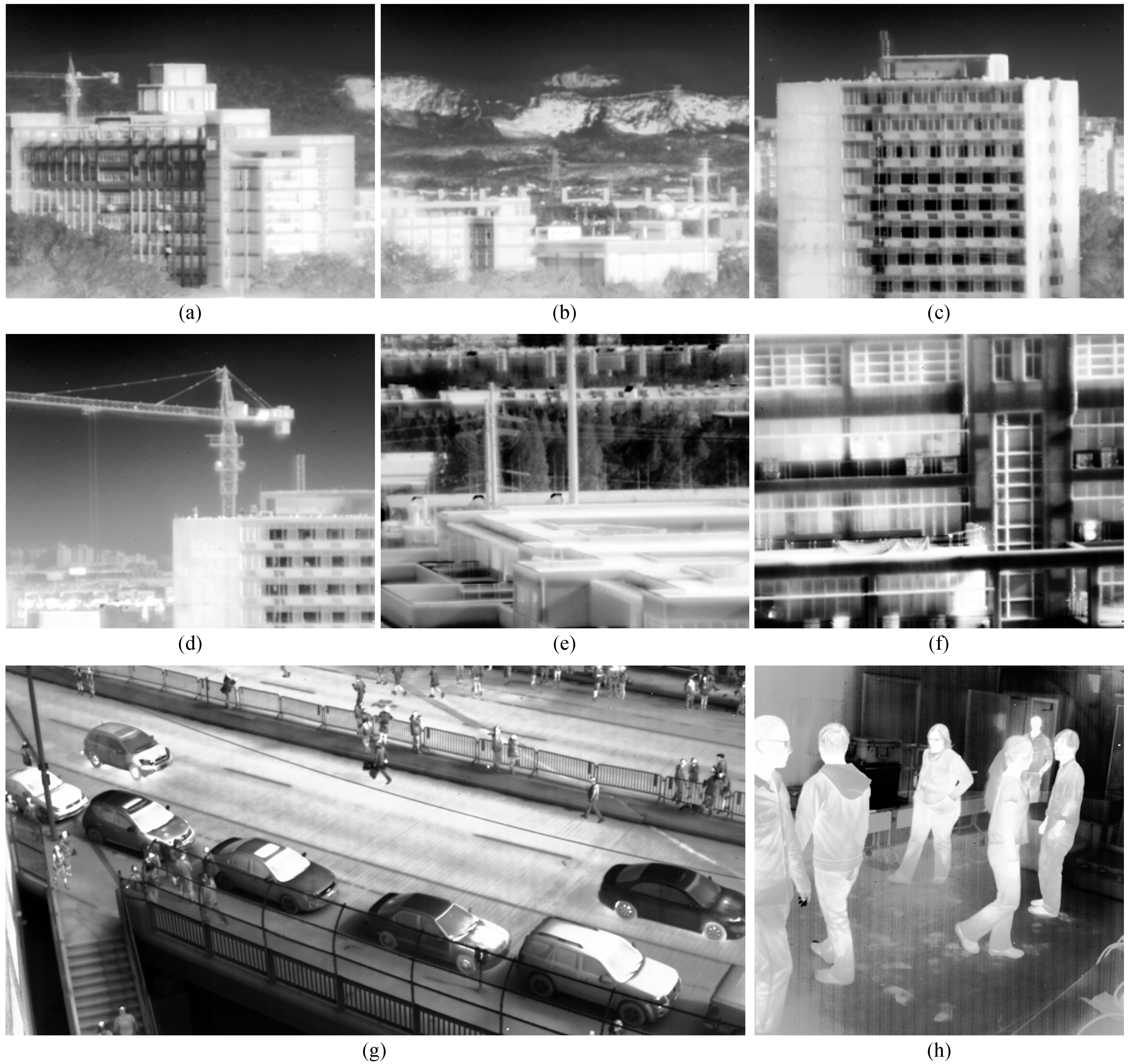
In this section, we apply the proposed method to six captured 14-bit infrared images and two raw infrared images extracted from the video sequences in BU-TIV [38] to evaluate its performance. The imager we used to capture the six infrared images is developed by our lab based on the sensor MARS-LW-RM3 with resolution $320\times 256$ and is sensitive to the long-wave band $8-10 \mathsf{\mu }\mathrm{m}$. The resolution of the other two raw infrared images is $1024\times 512$ and $512\times 512$. Figure 6 shows the HE results of the eight infrared images as a reference. In our experiments, the results are compared with those of four other block-based well-designed contrast enhancement methods: CLAHE, BCCE, ABMHE, and LGGSF. All of the experiments are conducted using MATLAB on a PC with Intel(R) Core(TM) i5 CPU (3.2 GHz) and 16GB RAM on a Windows 7 operating system.

4.1. The setting of Block Size and Threshold $t$

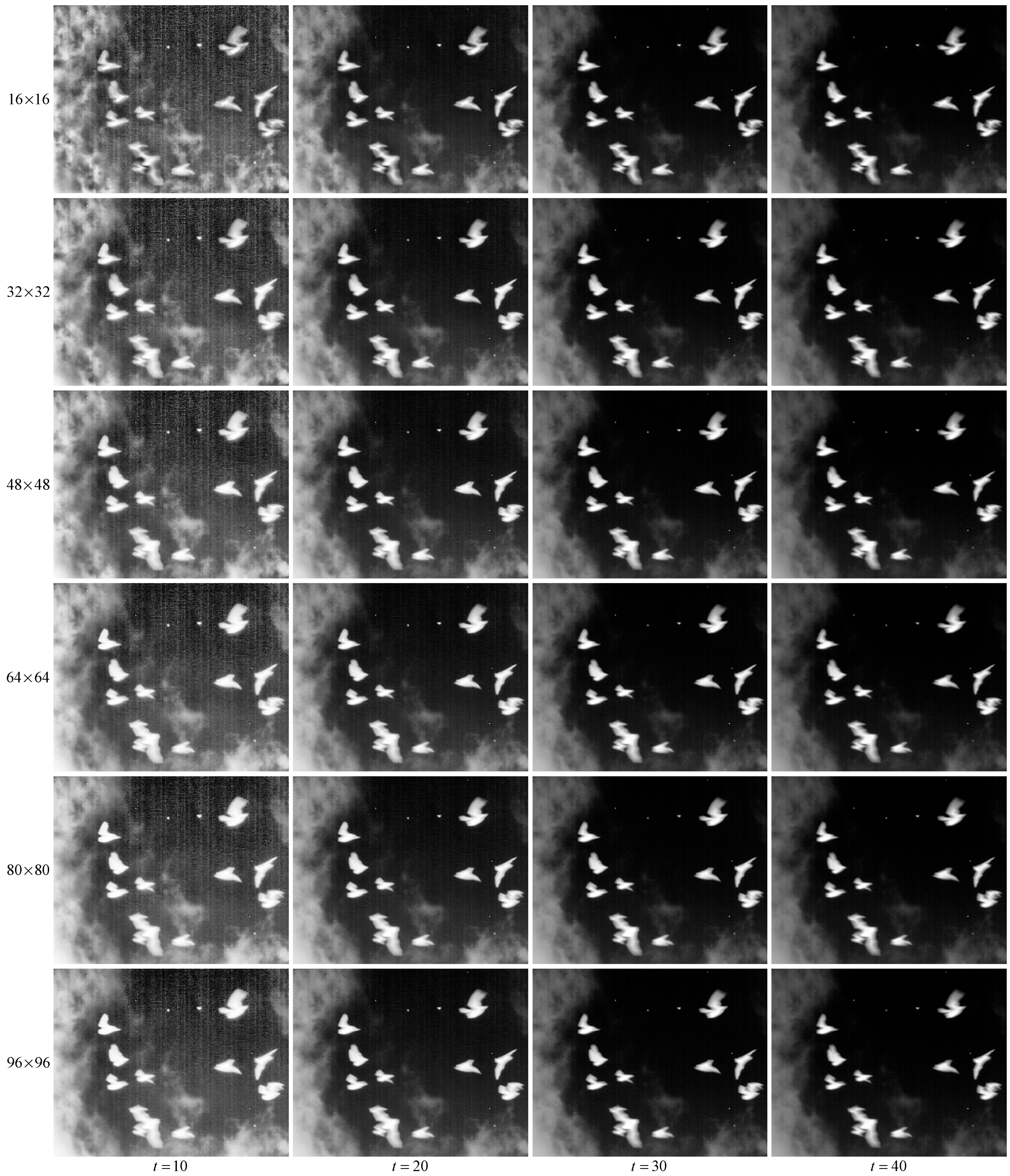
In this section, we conduct a further discussion on the block size and the threshold $t$. The block size is introduced to determine the size of each block in CLAHE, and the threshold $t$ is introduced to compute the neighborhood conditional histogram in Equation (7). The proposed method is applied to a test image extracted from one image in BU-TIV with the resolution $320\times 256$ to analyze the influence of different parameter settings to the enhanced result. The enhanced results with different block size and the threshold $t$ are given in Figure 7. It can be seen that the nonuniformity of the test image is also enhanced when we set $t=10$. As $t$ increases, the nonuniformity of the enhanced results is gradually suppressed, and some tiny details are also lost. Therefore, when determining the value of the threshold $t$, we should make a compromise between noise suppression and tiny detail preservation. For the block size, some artifacts appear in the enhanced result when the size of each block is set to be $16\times 16$. As the block size increases, the local contrast enhancement is not as good as that obtained by small block size, but this contrast enhancement reduction is not obvious when the threshold $t$ is set to be a large value. In our experiments, we empirically set the block size to be $64\times 64$. For other infrared images with different resolution, the block size can also be set as $64\times 64$ or another value, but not too small. For the six test images we captured, the threshold is set as $t=10$ to get better local contrast enhancement. And for the other test images from BU-TIV, we set $t=20$ for the suppression of nonuniformity.

4.2. Qualitative Evaluation

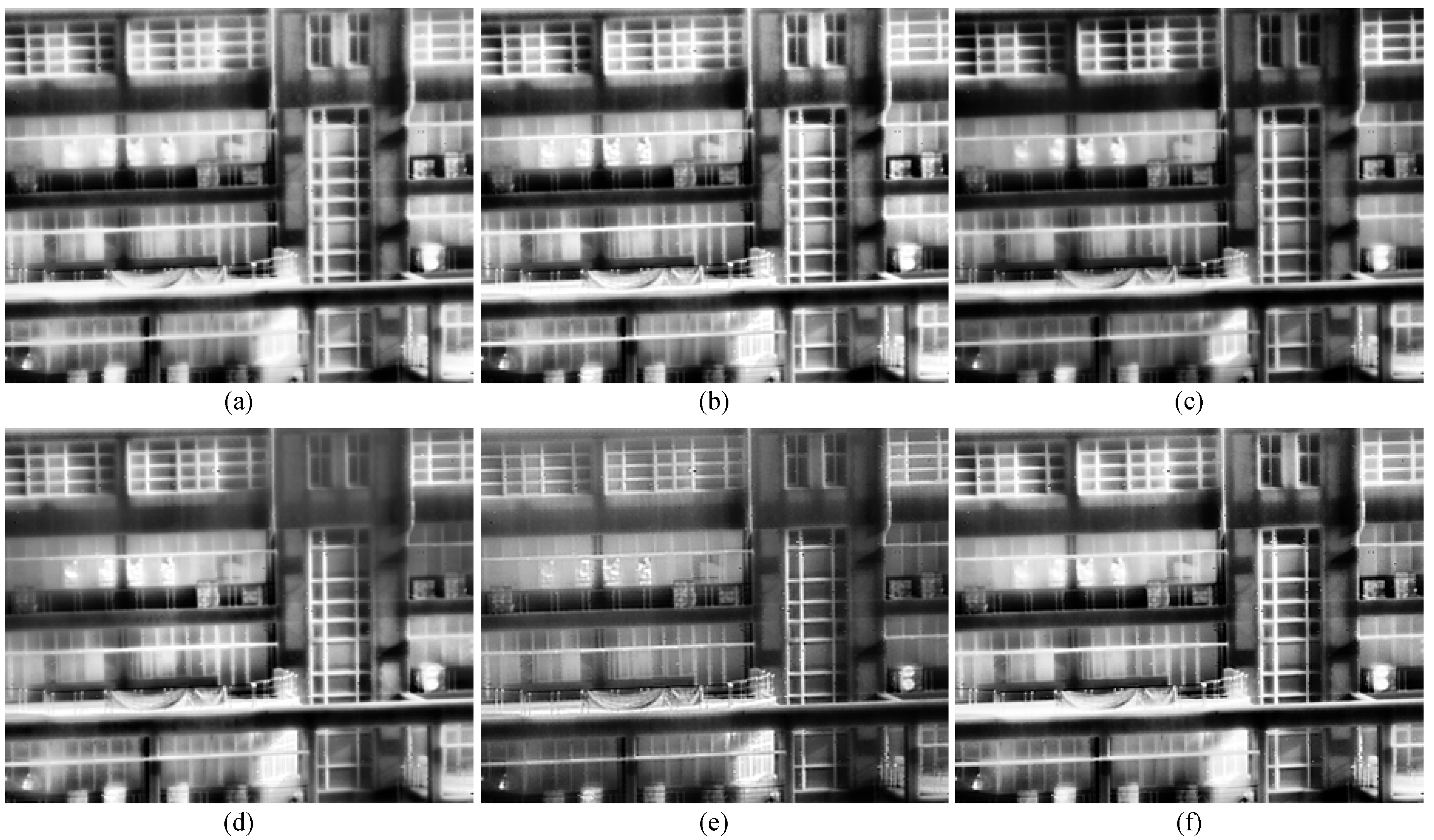
The experimental results of the infrared images are given in Figure 8, Figure 9, Figure 10, Figure 11, Figure 12 and Figure 13. The results are obtained by applying CLAHE, BCCE, ABMHE, LGGSF, and the proposed method to the infrared images. In addition to these, the intermediate enhanced results of the proposed method, and the enhanced results of the improved CLAHE are given together for comparison. The block size in CLAHE, BCCE, ABMHE, and the proposed method is set to be $64\times 64$. The number of divisions in horizontal and vertical of the image for LGGSF is set to be $k_x=k_y=7$ according to the original paper. In CLAHE and BCCE, the clip factor is set as $\alpha =0.01$. In addition, the local contrast enhancement factors for BCCE and LGGSF are set as $c=8$. Lastly, for ABMHE, the step size of the partially overlapped in horizontal and vertical is set to be one-quarter of the block size. For good enhancement results, they should obtain better local contrast enhancement and noise suppression, be artifact-free and visually pleasing.

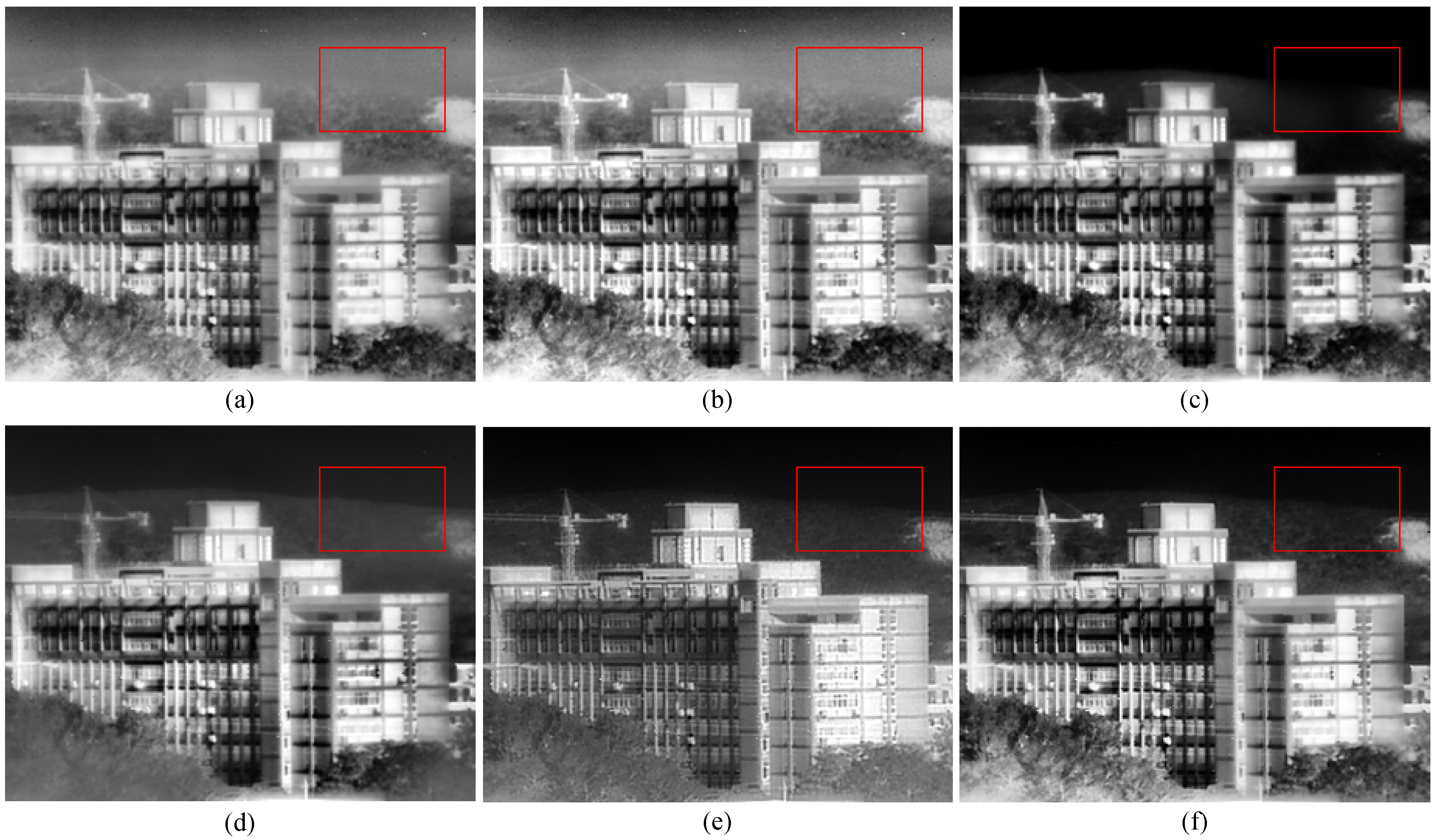
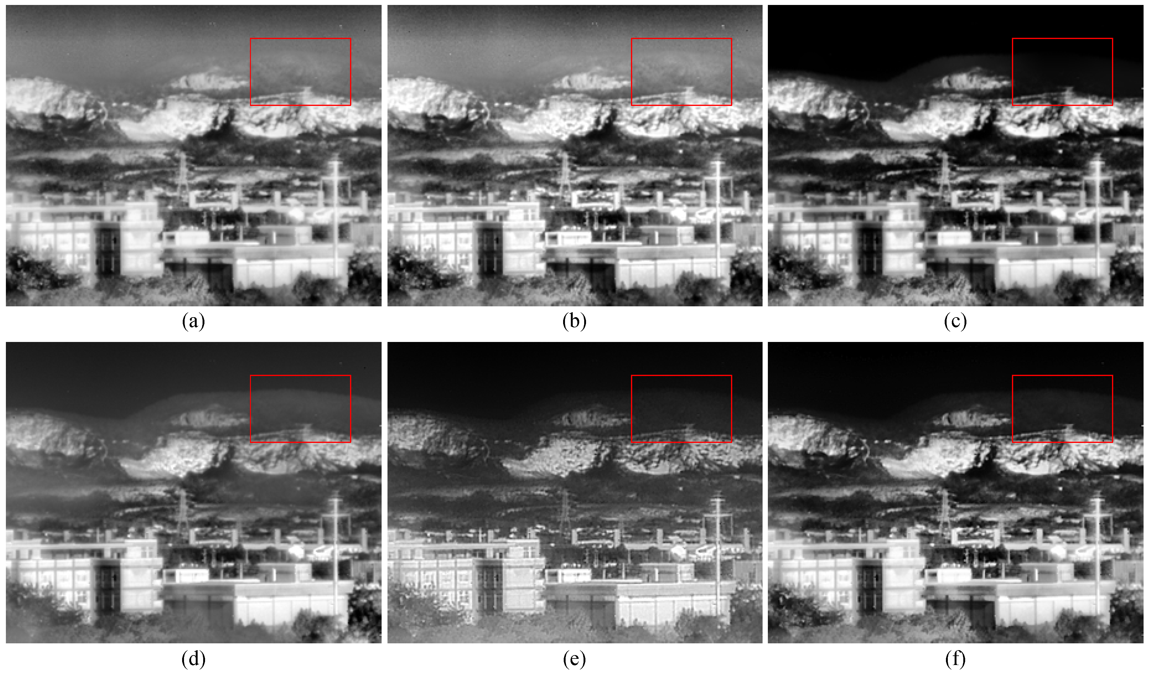
As shown in Figure 8, the enhanced results of CLAHE, BCCE, ABMHE, LGGSF, and the proposed method appear similar with respect to the building. CLAHE and BCCE cause noise amplification in the sky, which greatly reduces their performance compared with the other methods. ABMHE and LGGSF lost some details, as shown in the region marked by the red rectangle. This is caused by the improper classification in the transition region between the detail region and homogeneous region. The partial boundary of the mountain disappears in the ABMHE result, and some details of the trees in the LGGSF result also lost. All these undesired performance reductions do not appear in the enhanced result of GLHS and the proposed method. However, it is clear that the proposed method gets better local contrast enhancement than GLHS.

In Figure 9, the undesired noise amplification still appears in the enhanced result of CLAHE and BCCE. The details of the hills and buildings in BCCE result look clearer than those in the CLAHE result. Some part of the hills in the region marked by the red rectangle in the enhanced result of ABMHE cannot be distinguished from the sky. In the enhanced result of LGGSF, many details of the hills and the trees are smoothed. The local contrast enhancement of GLHS result is not as good as that of the other methods. Our proposed method produces a much better appearance and the finest details than the other methods.

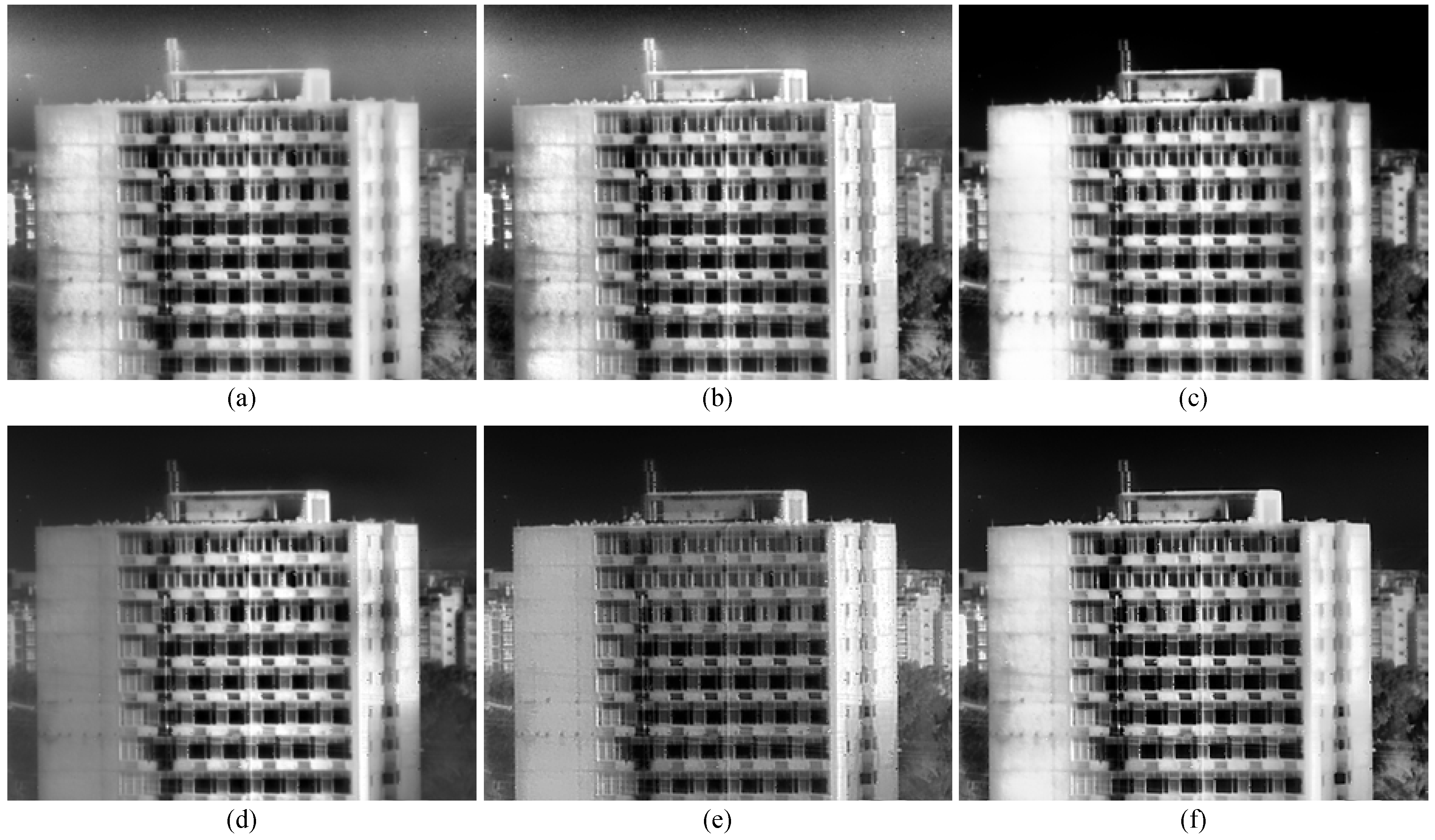
In Figure 10, CLAHE and BCCE still enhance the noise in the region of the sky. ABMHE obtains relatively good enhanced results for there is no transition region between the building and the sky, which is the same situation as the experiments in the original paper. In the enhanced result of LGGSF, the details of the trees in the left and right of the subgraph are still smoothed. Once again, GLHS does not produce better local contrast enhancement, and the proposed method outperforms the other methods with no artifacts, good appearance, and fine details.

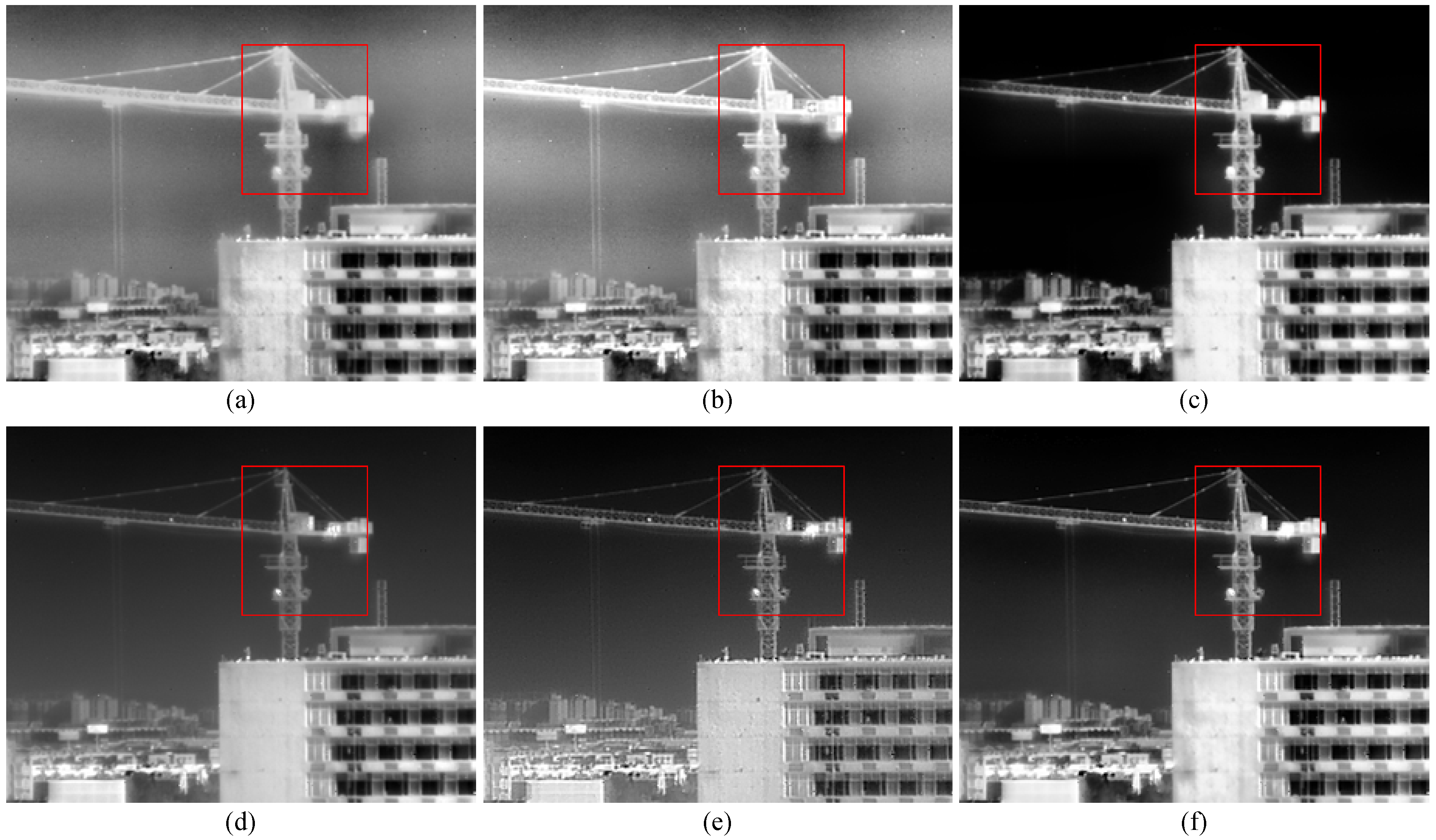
In Figure 11, the enhanced results of CLAHE and BCCE look unnatural due to the enhancement of noise and the appearance of block artifacts. As observed in the region marked by the red rectangle in the enhanced results of CLAHE, BCCE, and ABMHE, there are non-uniform brightness regions in the sky around the tower crane. These unpleasant appearance reductions cannot be found in the enhanced result of GLHS, LGGSF, and the proposed method. However, the details of the buildings and the tower crane do not look clearer than those of GLHS or the proposed method. In the homogeneous regions of the enhanced result of GLHS, some granular noise appears. The proposed produces an enhanced result with better visual quality improvement.

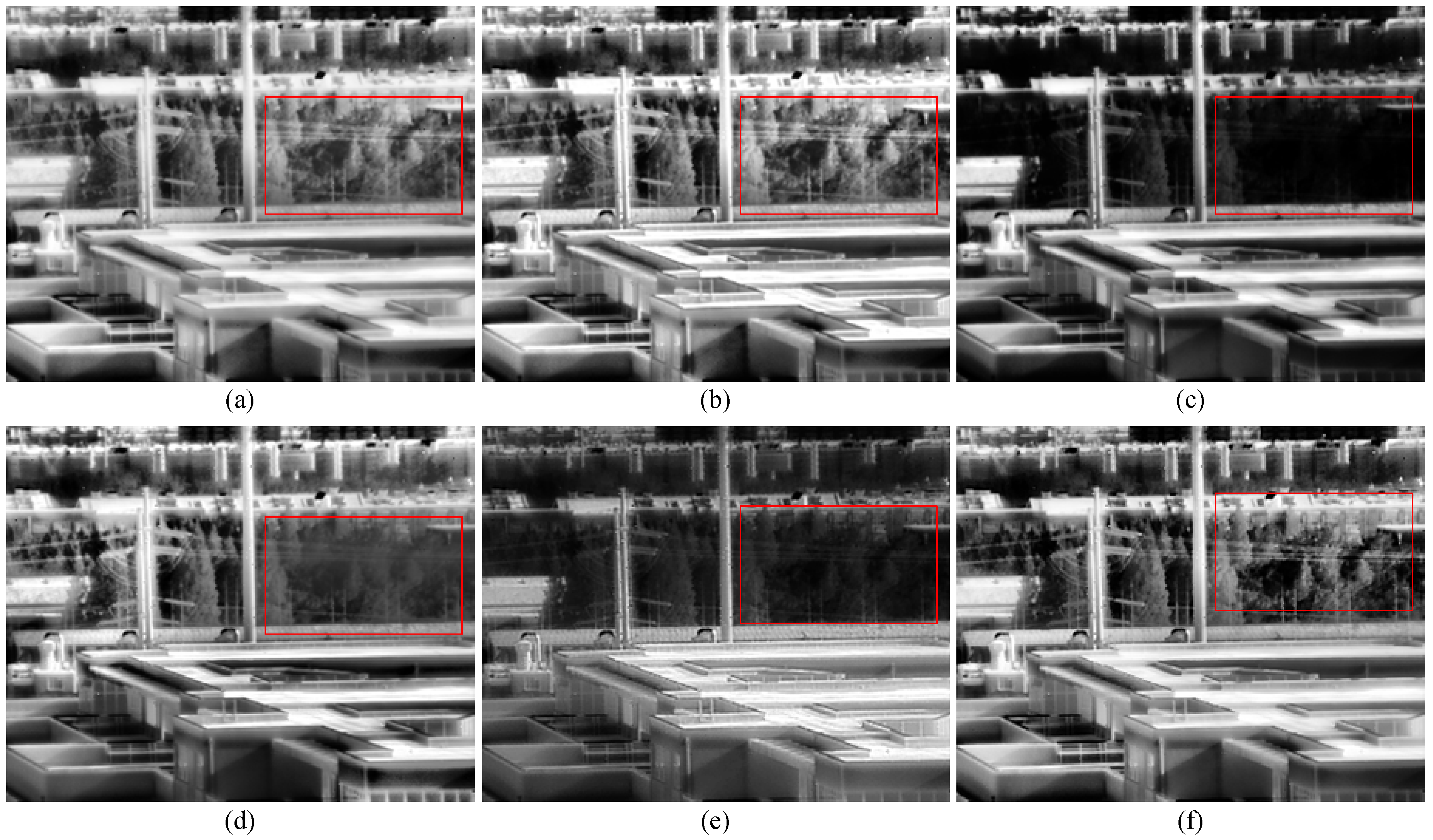
In Figure 12, CLAHE and BCCE produce better enhanced results than ABMHE, LGGSF, and GLHS, which benefits from the absence of the homogeneous region. As shown in the regions marked by the red rectangles in the enhanced results of ABMHE and LGGSF, many details of the trees are lost. This is caused by the improper classification of this low contrast region. The enhanced result of the proposed method looks better than that of BCCE, for the local contrast is well enhanced.

In Figure 13, the enhanced results of CLAHE, BCCE, ABMHE, LGGSF, and the proposed method resemble each other. The enhanced result of GLHS looks clear, but the local contrast is not well enhanced. Local contrast in the enhanced results of the proposed method and BCCE appears better than that of the other methods.

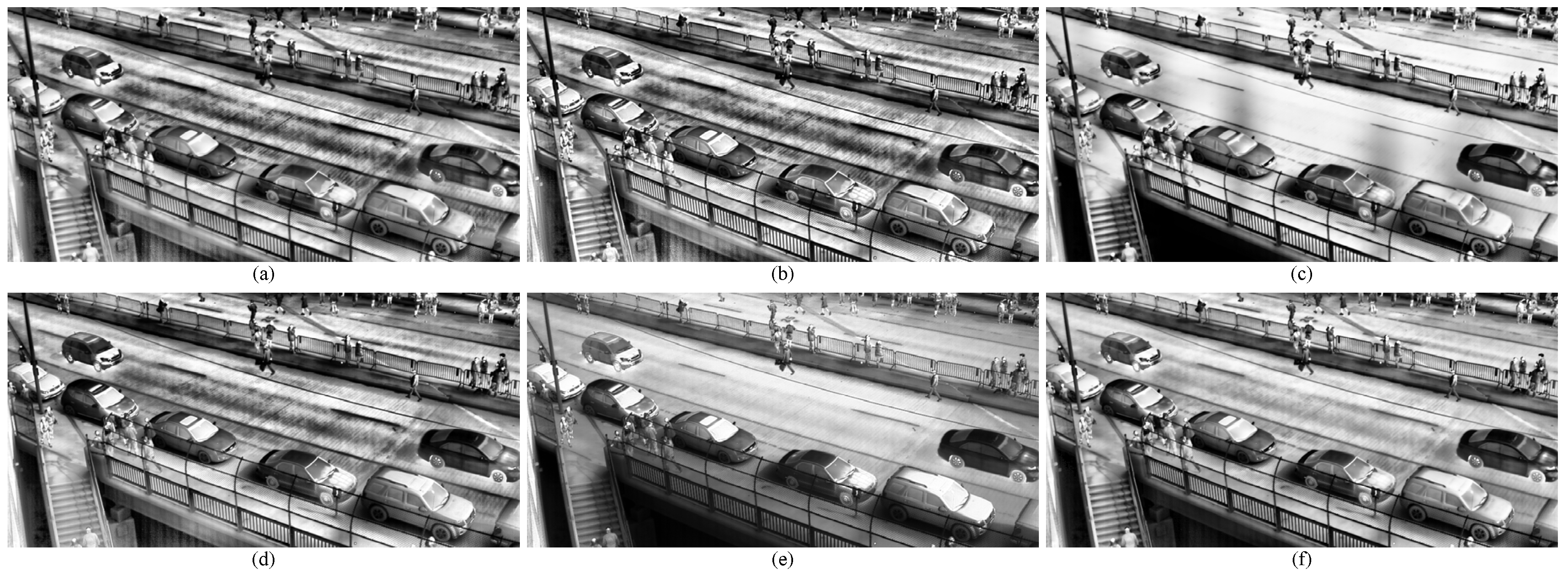
In Figure 14, due to the existence of nonuniformity, the enhanced results of CLAHE, BCCE, and LGGSF look poor because they are sensitive to the nonuniformity. In the enhanced result of ABMHE, there are non-uniform brightness regions in the road. GLHS performs best in terms of nonuniformity suppression. However, the local contrast is not well enhanced. The proposed method is able to suppress the nonuniformity and get better local contrast enhancement.

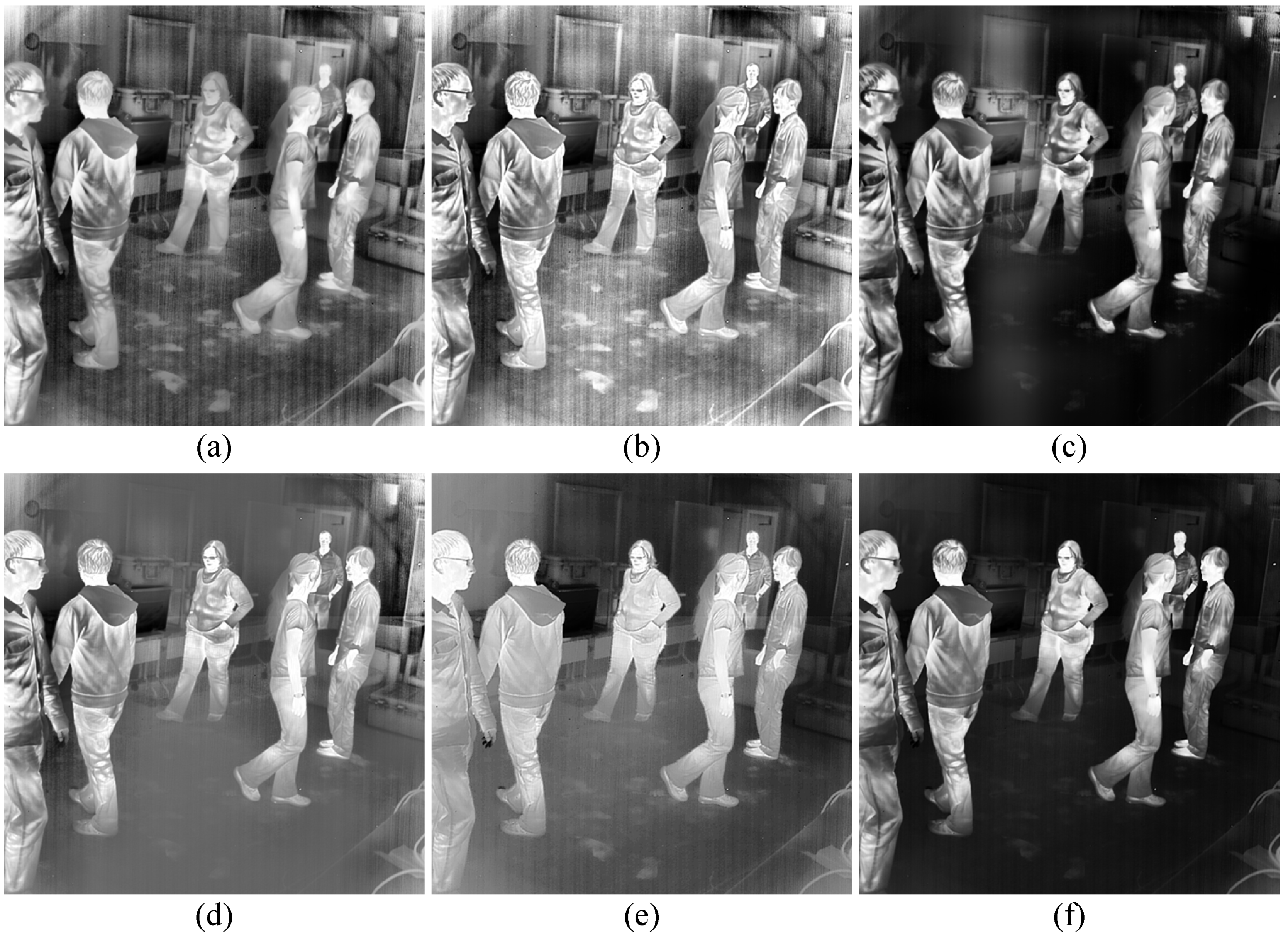
In Figure 15, the enhanced results of CLAHE and BCCE look terrible for the enhancement of the nonuniformity. The nonuniformity is well suppressed in the enhanced result of ABMHE, but there exists non-uniform brightness. The nonuniformity is suppressed in some regions of the LGGSF result. GLHS performs well on the nonuniformity suppression, but the local contrast is not well enhanced. The proposed method produces a better enhanced result with a natural appearance and nonuniformity suppression.

4.3. Quantitative Evaluation

In this section, to evaluate the performance of the six methods objectively, four metrics are adopted in this paper. They are the measure of enhancement by entropy (EMEE) [39], structural index (SI) [40], no-reference structural sharpness (NRSS) [41], and the lightness order error (LOE) [42].

EMEE is defined based on the Weber contrast and the concept of entropy, which is computed by the equation below.

$$EMEE(I)=\frac{1}{k_1{k}_2}{\displaystyle \sum _{k=1}^{k_1}{\displaystyle \sum _{l=1}^{k_2}\alpha {\left[\frac{I_{k,l}^{\max }}{I_{k,l}^{\min }+c}\right]}^{\alpha }\ln \left[\frac{I_{k,l}^{\max }}{I_{k,l}^{\min }+c}\right]}},$$

(23)

where $k_1$ and $k_2$ are the number of divisions in horizontal and vertical of the given image $I$, $I_{k,l}^{\max }$ and $I_{k,l}^{\min }$ represent the maximum and minimum values of the block $(k,l)$, respectively, $\alpha$ is an additional parameter, and $c$ is a small constant introduced to avoid dividing by zero. Generally, a larger EMEE value implies a higher contrast of the given image. In this paper, we set $\alpha =0.2$, $c=0.0001$, and the block size is $8\times 8$.

SI is defined based on the correlation coefficient, and the expression is given below.

$$SI(X,Y)=\frac{{\sigma }_{X,Y}+c}{{\sigma }_X{\sigma }_Y+c}.$$

(24)

where $X$ and $Y$ represent the input image and the enhanced image, ${\sigma }_{X,Y}$ is the covariance of $X$ and $Y$, ${\sigma }_X$ and ${\sigma }_Y$ are the standard deviation, $c$ is a small constant introduced to avoid dividing by zero, and ${\sigma }_{X,Y}$ is computed by the equation below.

$${\sigma }_{X,Y}=\frac{1}{N-1}{\displaystyle \sum _{i=1}^N(I_X(i)-{\mu }_{I_X})(I_Y(i)-{\mu }_{I_Y})},$$

(25)

where $N$ is the number of pixels in the images, ${\mu }_{I_X}$ and ${\mu }_{I_Y}$ are, respectively, the mean intensity of $I_X$ and $I_Y$. It is clear that SI indicates the global structural similarity of the enhanced image when compared to the input image. A larger SI value means that there is a high similarity between the enhanced image and the input image in terms of structure.

NRSS is defined based on the well-known SSIM (structural similarity index measurement) [43]. It indicates the structural sharpness of the given image and is computed by the equation below.

$$NRSS(I)=1-\frac{1}{K}{\displaystyle \sum _{i=1}^{K}SSIM(B_i^{G_I},B_i^{G_{F(I)}})},$$

(26)

where $B_i^{G_I}$ and $B_i^{G_{F(I)}}$ are one of the $K$ overlapped sub-blocks with higher variations in $G_I$ and $G_{F(I)}$, $G_I$ represents the gradient image and is computed by applying the Sobel operator to the given image $I$, and $G_{F(I)}$ is the gradient image of the Gaussian-blurred image $F(I)$. A large NRSS value means that the given image looks clear with high contrast. In this paper, the block size in NRSS is set to be $32\times 32$, the step size is set to be half of the block size, and $K$ is equal to half of the total number of the overlapped sub-blocks.

LOE is defined to indicate the lightness order error between the input image and the enhanced image. The expression of LOE is given below.

$$\{\begin{array}{l}LOE=\frac{1}{AB}{\displaystyle \sum _{a=1}^A{\displaystyle \sum _{b=1}^{B}R{D}_{a,b}}}\hfill \\ R{D}_{a,b}={\displaystyle \sum _{m=1}^A{\displaystyle \sum _{n=1}^B\left[U(X_{a,b}^D,X_{m,n}^D)\oplus U(Y_{a,b}^D,Y_{m,n}^D)\right]}}\hfill \\ U(x,y)=\{\begin{array}{l}\begin{array}{cc}1,& forx\ge y\end{array}\hfill \\ \begin{array}{cc}0,& else\end{array}\hfill \end{array}\hfill \end{array},$$

(27)

where $A\times B$ represents the image size of $X^D$ and $Y^D$, $U(x,y)$ is the unit step function, $\oplus$ is the exclusive or operator, $X^D$ and $Y^D$ are the down-sampled versions of $X$ and $Y$ to reduce the computational complexity. The ratio between the size of the input image and that of the down-sampled image is set as $r=16$ in this paper. Obviously, a small LOE value indicates that the enhanced image gets better naturalness preservation of the input image.

In

Table 1. The quantitative evaluation results of contrast-limited adaptive histogram equalization (CLAHE), balanced CLAHE and contrast enhancement (BCCE), adjacent-blocks-based modification for local histogram equalization (ABMHE), local gradient-grayscale statistical feature (LGGSF), global and local histogram specification (GLHS), and the proposed method in terms of enhancement by entropy (EMEE), structural index (SI), no-reference structural sharpness (NRSS), and lightness order error (LOE).

Metrics	Methods	Infrared Images in the Experiments								Average
		Building1	Hills	Building2	Sky	Trees	Windows	Road	Students
EMEE	CLAHE	0.2000	0.1963	0.5770	0.3317	0.4823	0.5753	1.4999	0.3592	0.5277
	BCCE	0.4388	0.4486	0.7091	0.6456	1.0899	1.5121	1.8979	0.4839	0.9032
	ABMHE	1.4180	1.8156	1.6300	1.8697	2.5899	1.4987	1.6859	0.7242	1.6540
	LGGSF	0.2960	0.2153	0.6360	0.1497	1.2646	0.9432	1.1786	0.1701	0.6067
	GLHS	0.3809	0.2377	2.8797	0.4055	1.5728	1.9295	0.5263	0.3730	1.0382
	Proposed	3.3892	1.8031	5.5496	2.1652	5.9257	4.8795	2.5674	0.8721	3.3940
SI	CLAHE	0.6873	0.6851	0.6887	0.6885	0.6569	0.8021	0.6476	0.7586	0.7019
	BCCE	0.6449	0.6388	0.6672	0.5907	0.6476	0.7943	0.6197	0.5595	0.6453
	ABMHE	0.7930	0.8563	0.6541	0.9103	0.7924	0.8197	0.8676	0.8211	0.8143
	LGGSF	0.8347	0.9283	0.7537	0.9778	0.6575	0.8341	0.7031	0.8551	0.8180
	GLHS	0.9577	0.9494	0.8608	0.9793	0.9027	0.9211	0.9761	0.9094	0.9321
	Proposed	0.8607	0.8996	0.7503	0.9625	0.7247	0.8490	0.8999	0.9520	0.8623
NRSS	CLAHE	0.8704	0.8442	0.8535	0.8483	0.7960	0.7682	0.7734	0.8115	0.8207
	BCCE	0.9237	0.9038	0.9092	0.8981	0.8609	0.8202	0.8723	0.8806	0.8836
	ABMHE	0.8578	0.8343	0.8425	0.8263	0.7780	0.8141	0.7656	0.7856	0.8130
	LGGSF	0.8925	0.8797	0.8748	0.8770	0.8474	0.8257	0.8491	0.8684	0.8643
	GLHS	0.9613	0.9583	0.9398	0.9352	0.8997	0.9055	0.8771	0.8851	0.9203
	Proposed	0.9160	0.8988	0.9124	0.8879	0.8660	0.8558	0.8102	0.8349	0.8728
LOE	CLAHE	73.89	87.27	64.98	97.09	70.73	43.24	523.51	257.11	152.23
	BCCE	79.95	89.96	68.28	104.92	74.46	44.77	544.24	324.97	166.44
	ABMHE	42.46	41.41	44.83	51.38	39.90	48.97	338.67	241.06	106.09
	LGGSF	34.68	35.15	35.38	9.67	82.74	41.20	463.96	201.55	113.04
	GLHS	11.26	9.5156	9.08	8.75	10.13	10.35	63.04	28.01	18.77
	Proposed	23.47	26.44	25.78	17.56	53.64	29.90	274.76	94.67	68.28

, the quantitative evaluation results of the six methods in terms of the four metrics are given. The highest results of EMEE, SI, and NRSS, the lowest results of LOE are marked in bold in the table. Among these methods, the other five methods except GLHS are block-based methods, and the foundation of GLHS is global histogram specification. Therefore, GLHS usually gets the highest SI values and the lowest LOE values. The proposed method provides almost the highest EMEE values, except in Hills. Although the EMEE value of the proposed method in Hills is slightly smaller than that of ABMHE, the proposed method provides the highest average EMEE value among the five methods. For the SI values, due to the utilization of block-based local contrast enhancement, the SI values of the five block-based methods are lower than those of GLHS. The proposed method usually gives relatively higher SI values among the block-based methods, and the average SI value of the proposed method is the highest in the five block-based methods. This means the proposed method performs well on the structural similarity with the input image. Benefitting from the local contrast enhancement process, the NRSS values of GLHS are the highest among the six methods. For the first six infrared images, the proposed method usually produces relatively high NRSS values. Whereas for the other two test infrared images, the NRSS values of the proposed method are not as high as those of BCCE and LGGSF, this is caused by the setting of the higher threshold. The reason why the NRSS values are not the highest among the methods is the combination of both global and local enhanced results when enhancing the local contrast. Comparison of LOE values indicates that the proposed method almost provides the lowest values among the five block-based methods, except in Sky and Trees. However, the average LOE value of the proposed method is obviously the lowest among that of the other block-based methods. In summary, the values of the four metrics demonstrate that the proposed method outperforms the other five methods in terms of local contrast enhancement and performs well on the structural similarity, detail improvement, and naturalness preservation.

In

Table 2. The average time consumption of the six methods on the six captured test images (Unit: Second).

Method	CLAHE	BCCE	ABMHE	LGGSF	GLHS	Proposed
Time	0.0675	0.0842	3.2471	0.1522	0.9172	0.1674

, the average time consumption for the six methods to process the six captured test images are given. It is clear that the time computation of CLAHE and BCCE is lower than those of the other three methods. The local contrast enhancement process of BCCE leads to a higher computation time than CLAHE. Due to the utilization of sub-block classification and labeling, LGGSF needs more computation time than BCCE. The computation time of the proposed method is higher than LGGSF and BCCE, this is caused by the computation of neighborhood conditional histogram in each sub-block and the optimized contrast enhancement process. For the GLHS, the utilization of the 2D histogram, histogram specification, and the local contrast enhancement process lead to a more time-consuming process. In ABMHE, the large amount of overlapped sub-blocks and the sub-block searching operations make it a computationally expensive method. Therefore, its consumption time is the highest among the six methods.

5. Conclusions

In this paper, to improve the visual quality of infrared images, we proposed an adaptive contrast enhancement method based on the neighborhood conditional histogram. We introduced the neighborhood conditional histogram into CLAHE to avoid over-enhancement and achieve adaptive contrast enhancement for various sub-blocks. To eliminate the block-artifacts, the mapping functions are further updated based on the global mapping function. Lastly, the local contrast is optimized based on both global and local enhanced result, and then adaptively enhanced based on the edge information of the input image. The neighborhood conditional histogram and the strategy that combines both global and local mapping functions to reduce the block artifacts and enhance the local contrast are the main innovations of this paper. By setting different parameters for the neighborhood conditional, the proposed method is able to adaptively enhance the local contrast and suppress the nonuniformity of the input infrared images. In addition, the proposed method has the potential to be implemented on the hardware platform, such as FPGA. Therefore, the proposed method can be applied to the infrared imaging system to improve performance.

References

- Weng, Q. Thermal infrared remote sensing for urban climate and environmental studies: Methods, applications, and trends. ISPRS J. Photogramm. Remote Sens. 2009, 64, 335–344. [Google Scholar] [CrossRef]
- Cao, Y.; Yang, M.Y.; Tisse, C.L. Effective Strip Noise Removal for Low-Textured Infrared Images Based on 1-D Guided Filtering. IEEE Trans. Circuits Syst. Video Technol. 2016, 26, 2176–2188. [Google Scholar] [CrossRef]
- Ring, E.; Ammer, K. Infrared thermal imaging in medicine. Physiol. Meas. 2012, 33, R33. [Google Scholar] [CrossRef]
- Liu, C.; Sui, X.; Liu, Y.; Kuang, X.; Gu, G. FPN estimation based nonuniformity correction for infrared imaging system. Infrared Phys. Technol. 2018, 96, 22–29. [Google Scholar] [CrossRef]
- Sun, X.; Liu, X.; Tang, Z.; Long, G.; Yu, Q. Real-time visual enhancement for infrared small dim targets in video. Infrared Phys. Technol. 2017, 83, 217–226. [Google Scholar] [CrossRef]
- Kim, J.-H.; Kim, J.-H.; Jung, S.-W.; Ko, S.-J.; Noh, C.-K. Novel contrast enhancement scheme for infrared image using detail-preserving stretching. OPTICE 2011, 50, 077002. [Google Scholar] [CrossRef]
- Huang, J.; Ma, Y.; Zhang, Y.; Fan, F. Infrared image enhancement algorithm based on adaptive histogram segmentation. Appl. Opt. 2017, 56, 9686–9697. [Google Scholar] [CrossRef] [PubMed]
- Gonzalez, R.C.; Woods, R.E.; Eddins, S.L. Digital Image Processing Using MATLAB; Pearson-Prentice-Hall: Upper Saddle River, NJ, USA, 2004; Volume 624. [Google Scholar]
- Song, K.S.; Kang, M.G. Optimized Tone Mapping Function for Contrast Enhancement considering Human Visual Perception System. IEEE Trans. Circuits Syst. Video Technol. 2018. [Google Scholar] [CrossRef]
- Lin, C.-L. An approach to adaptive infrared image enhancement for long-range surveillance. Infrared Phys. Technol. 2011, 54, 84–91. [Google Scholar] [CrossRef]
- Vickers, V.E. Plateau equalization algorithm for real-time display of high-quality infrared imagery. OPTICE 1996, 35, 1921–1927. [Google Scholar] [CrossRef]
- Wang, B.-J.; Liu, S.-Q.; Li, Q.; Zhou, H.-X. A real-time contrast enhancement algorithm for infrared images based on plateau histogram. Infrared Phys. Technol. 2006, 48, 77–82. [Google Scholar] [CrossRef]
- Liang, K.; Ma, Y.; Xie, Y.; Zhou, B.; Wang, R. A new adaptive contrast enhancement algorithm for infrared images based on double plateaus histogram equalization. Infrared Phys. Technol. 2012, 55, 309–315. [Google Scholar] [CrossRef]
- Li, S.; Jin, W.; Li, L.; Li, Y. An improved contrast enhancement algorithm for infrared images based on adaptive double plateaus histogram equalization. Infrared Phys. Technol. 2018, 90, 164–174. [Google Scholar] [CrossRef]
- Kim, Y.-T. Contrast enhancement using brightness preserving bi-histogram equalization. IEEE Trans. Consum. Electron. 1997, 43, 1–8. [Google Scholar]
- Wang, Y.; Chen, Q.; Zhang, B. Image enhancement based on equal area dualistic sub-image histogram equalization method. IEEE Trans. Consum. Electron. 1999, 45, 68–75. [Google Scholar] [CrossRef]
- Chen, S.-D.; Ramli, A.R. Contrast enhancement using recursive mean-separate histogram equalization for scalable brightness preservation. IEEE Trans. Consum. Electron. 2003, 49, 1301–1309. [Google Scholar] [CrossRef]
- Wan, M.; Gu, G.; Qian, W.; Ren, K.; Chen, Q.; Maldague, X. Infrared Image Enhancement Using Adaptive Histogram Partition and Brightness Correction. Remote Sens. 2018, 10, 682. [Google Scholar] [CrossRef]
- Arici, T.; Dikbas, S.; Altunbasak, Y. A histogram modification framework and its application for image contrast enhancement. IEEE Trans. Image Process. 2009, 18, 1921–1935. [Google Scholar] [CrossRef]
- Xiao, B.; Tang, H.; Jiang, Y.; Li, W.; Wang, G. Brightness and contrast controllable image enhancement based on histogram specification. Neurocomputing 2018, 275, 2798–2809. [Google Scholar] [CrossRef]
- Zuiderveld, K. Contrast limited adaptive histogram equalization. Graph. Gems 1994, 474–485. [Google Scholar]
- Kim, J.-Y.; Kim, L.-S.; Hwang, S.-H. An advanced contrast enhancement using partially overlapped sub-block histogram equalization. IEEE Trans. Circuits Syst. Video Technol. 2001, 11, 475–484. [Google Scholar]
- Branchitta, F.; Diani, M.; Corsini, G.; Porta, A. Dynamic-range compression and contrast enhancement in infrared imaging systems. OPTICE 2008, 47, 076401. [Google Scholar] [CrossRef]
- Wang, Y.; Pan, Z. Image contrast enhancement using adjacent-blocks-based modification for local histogram equalization. Infrared Physics Technol. 2017, 86, 59–65. [Google Scholar] [CrossRef]
- Li, S.; Jin, W.; Wang, X.; Li, L.; Liu, M. Contrast Enhancement Algorithm for Outdoor Infrared Images based on Local Gradient-grayscale Statistical Feature. IEEE Access 2018, 6. [Google Scholar] [CrossRef]
- Yuan, L.T.; Swee, S.K.; Ping, T.C. Infrared image enhancement using adaptive trilateral contrast enhancement. Pattern Recognit. Lett. 2015, 54, 103–108. [Google Scholar] [CrossRef]
- Branchitta, F.; Diani, M.; Corsini, G.; Romagnoli, M. New technique for the visualization of high dynamic range infrared images. OPTICE 2009, 48, 096401. [Google Scholar] [CrossRef]
- Zuo, C.; Chen, Q.; Liu, N.; Ren, J.; Sui, X. Display and detail enhancement for high-dynamic-range infrared images. OPTICE 2011, 50, 127401. [Google Scholar] [CrossRef]
- Li, Y.; Hou, C.; Tian, F.; Yu, H.; Guo, L.; Xu, G.; Shen, X.; Yan, W. Enhancement of infrared image based on the retinex theory. In Proceedings of the 2007 29th Annual International Conference of the IEEE Engineering in Medicine and Biology Society, Lyon, France, 22–26 August 2007; pp. 3315–3318. [Google Scholar]
- Zhan, B.; Wu, Y. Infrared image enhancement based on wavelet transformation and retinex. In Proceedings of the 2010 Second International Conference on Intelligent Human-Machine Systems and Cybernetics, Nanjing, China, 26–28 August 2010; pp. 313–316. [Google Scholar]
- Mallat, S.G. A theory for multiresolution signal decomposition: The wavelet representation. IEEE Trans. Pattern Anal. Mach. Intell. 1989, 11, 674–693. [Google Scholar] [CrossRef]
- Singh, R.; Khare, A. Fusion of multimodal medical images using Daubechies complex wavelet transform–A multiresolution approach. Inf. Fusion 2014, 19, 49–60. [Google Scholar] [CrossRef]
- Liu, C.; Sui, X.; Kuang, X.; Liu, Y.; Gu, G.; Chen, Q. Optimized Contrast Enhancement for Infrared Images Based on Global and Local Histogram Specification. Remote Sens. 2019, 11, 849. [Google Scholar] [CrossRef]
- Pizer, S.M.; Amburn, E.P.; Austin, J.D.; Cromartie, R.; Geselowitz, A.; Greer, T.; ter Haar Romeny, B.; Zimmerman, J.B.; Zuiderveld, K. Adaptive histogram equalization and its variations. Comput. Vis. Graph. Image Process. 1987, 39, 355–368. [Google Scholar] [CrossRef]
- Unal, B.; Akoglu, A. Resource efficient real-time processing of contrast limited adaptive histogram equalization. In Proceedings of the 2016 26th International Conference on Field Programmable Logic and Applications (FPL), Lausanne, Switzerland, 29 August–2 September 2016; pp. 1–8. [Google Scholar]
- Jenifer, S.; Parasuraman, S.; Kadirvelu, A. Contrast enhancement and brightness preserving of digital mammograms using fuzzy clipped contrast-limited adaptive histogram equalization algorithm. Appl. Soft Comput. 2016, 42, 167–177. [Google Scholar] [CrossRef]
- Chang, Y.; Jung, C.; Ke, P.; Song, H.; Hwang, J. Automatic Contrast Limited Adaptive Histogram Equalization with Dual Gamma Correction. IEEE Access 2018, 6, 11782–11792. [Google Scholar] [CrossRef]
- Wu, Z.; Fuller, N.; Theriault, D.; Betke, M. A thermal infrared video benchmark for visual analysis. In Proceedings of the IEEE Conference on Computer Vision and Pattern Recognition Workshops, Columbus, OH, USA, 23–28 June 2014; pp. 201–208. [Google Scholar]
- Panetta, K.; Gao, C.; Agaian, S. No reference color image contrast and quality measures. IEEE Trans. Consum. Electron. 2013, 59, 643–651. [Google Scholar] [CrossRef]
- Rivera, A.R.; Ryu, B.; Chae, O. Content-aware dark image enhancement through channel division. IEEE Trans. Image Process. 2012, 21, 3967–3980. [Google Scholar] [CrossRef] [PubMed]
- Xie, X.; Zhou, J.; Wu, Q. No-reference quality index for image blur. J. Comput. Appl. 2010, 30, 921–924. [Google Scholar] [CrossRef]
- Wang, S.; Zheng, J.; Hu, H.-M.; Li, B. Naturalness preserved enhancement algorithm for non-uniform illumination images. IEEE Trans. Image Process. 2013, 22, 3538–3548. [Google Scholar] [CrossRef]
- ZWang, Z. Image quality assessment from error measurement to structural similarity. IEEE Trans. Image Process. 2004, 13, 600r612. [Google Scholar]
Figure 1.
Histogram adjustment within sub-block (i, j).
Figure 2.
Diagram of the optimization problem.
Figure 3.
The enhancement result of the given infrared image using contrast-limited adaptive histogram equalization (CLAHE). (a) The histogram equalization (HE) result of the given image. (b) The CLAHE result of the given image. (c) The histogram of the given infrared image. (d) The histogram of each sub-block and the red line represents the clip limit. (e) The mapping function of HE and the mapping functions of sub-block 1, 2, and 3 in CLAHE. The X-axis ranges in (c–e) are set to be (9000,11,000) for better visualization.
Figure 4.
The enhanced result of the given infrared image. (a) The neighborhood conditional histogram of the given infrared image. (b) The corresponding enhanced result based on the neighborhood conditional histogram. The X-axis range in (a) is set to be (9000,11,000) for better visualization.
Figure 5.
The enhanced result of the given infrared image using the improved CLAHE. (a) The enhanced result. (b) The neighborhood conditional histogram of each sub-block and the red line is introduced to be a reference value of ten. (c) The global mapping function and the local mapping functions of sub-block 1, 2, and 3 in the improved CLAHE. The X-axis range in (b,c) are set to be (9000,11,000) for better visualization.
Figure 6.
The HE results of the six infrared images used in the experiments. (a) Building1, (b) Hills, (c) Building2, (d) Sky, (e) Trees, (f) Windows, (g) Road, (h) Students.
Figure 7.
The enhanced results of the proposed method with different parameter setting.
Figure 8.
Enhancement results for Building1. (a) contrast-limited adaptive histogram equalization (CLAHE), (b) balanced CLAHE and contrast enhancement (BCCE), (c) adjacent-blocks-based modification for local histogram equalization (ABMHE), (d) local gradient-grayscale statistical feature (LGGSF), (e) global and local histogram specification (GLHS), (f) Proposed.
Figure 9.
Enhancement results for Hills. (a) CLAHE, (b) BCCE, (c) ABMHE, (d) LGGSF, (e) GLHS, (f) Proposed.
Figure 10.
Enhancement results for Building2. (a) CLAHE, (b) BCCE, (c) ABMHE, (d) LGGSF, (e) GLHS, (f) Proposed.
Figure 11.
Enhancement results for Sky. (a) CLAHE, (b) BCCE, (c) ABMHE, (d) LGGSF, (e) GLHS, (f) Proposed.
Figure 12.
Enhancement results for Trees. (a) CLAHE, (b) BCCE, (c) ABMHE, (d) LGGSF, (e) GLHS, (f) Proposed.
Figure 13.
Enhancement results for Windows. (a) CLAHE, (b) BCCE, (c) ABMHE, (d) LGGSF, (e) GLHS, (f) Proposed.
Figure 14.
Enhancement results for Road. (a) CLAHE, (b) BCCE, (c) ABMHE, (d) LGGSF, (e) GLHS, (f) Proposed.
Figure 15.
Enhancement results for Students. (a) CLAHE, (b) BCCE, (c) ABMHE, (d) LGGSF, (e) GLHS. (f) Proposed.