A Sub-Regional Extraction Method of Common Mode Components from IGS and CMONOC Stations in China

 ,
,
Abstract
:
1. Introduction
2. Data and Methodology
2.1. Data
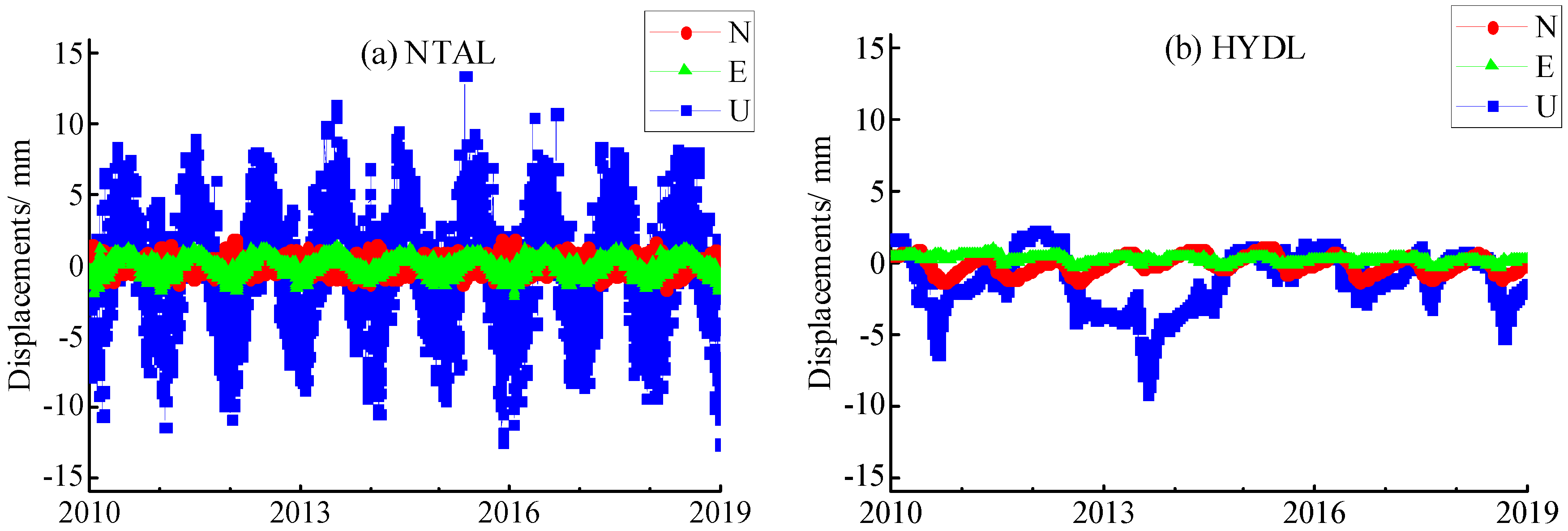
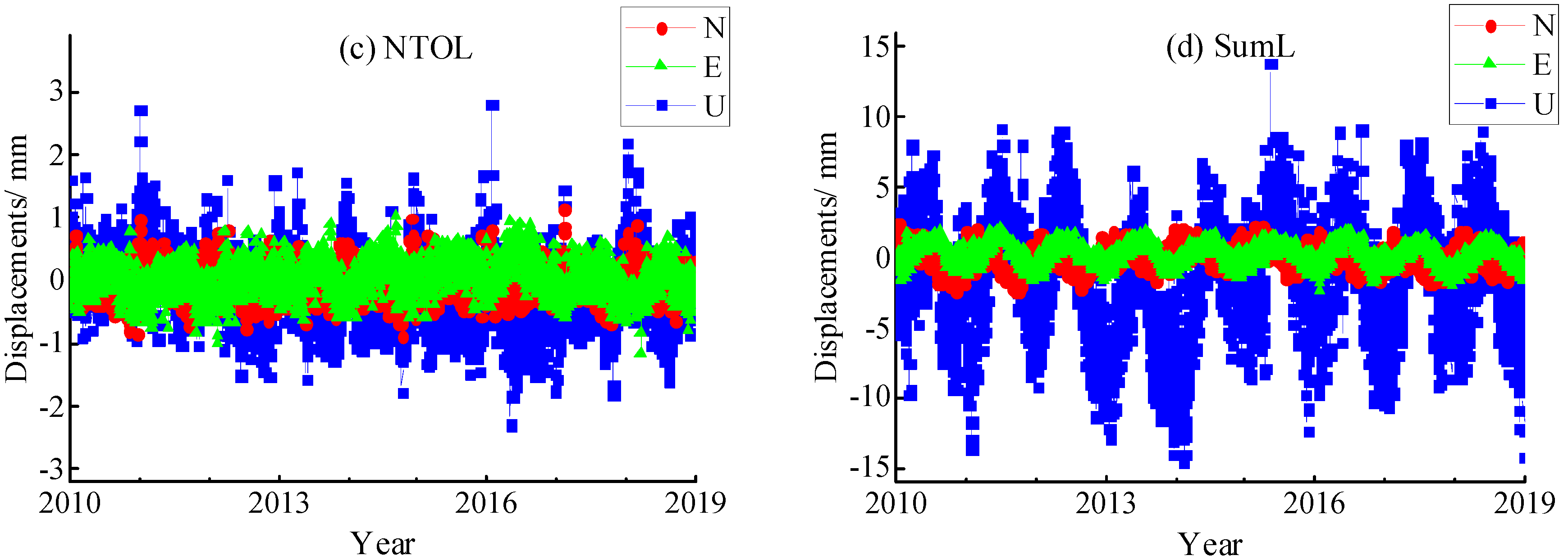
2.1.1. GPS Coordinate Time Series
2.1.2. Environmental Loading Data
2.2. Methodology
2.2.1. Acquisition of the Residual Time Series
2.2.2. Principal Component Analysis
3. CMC Extraction
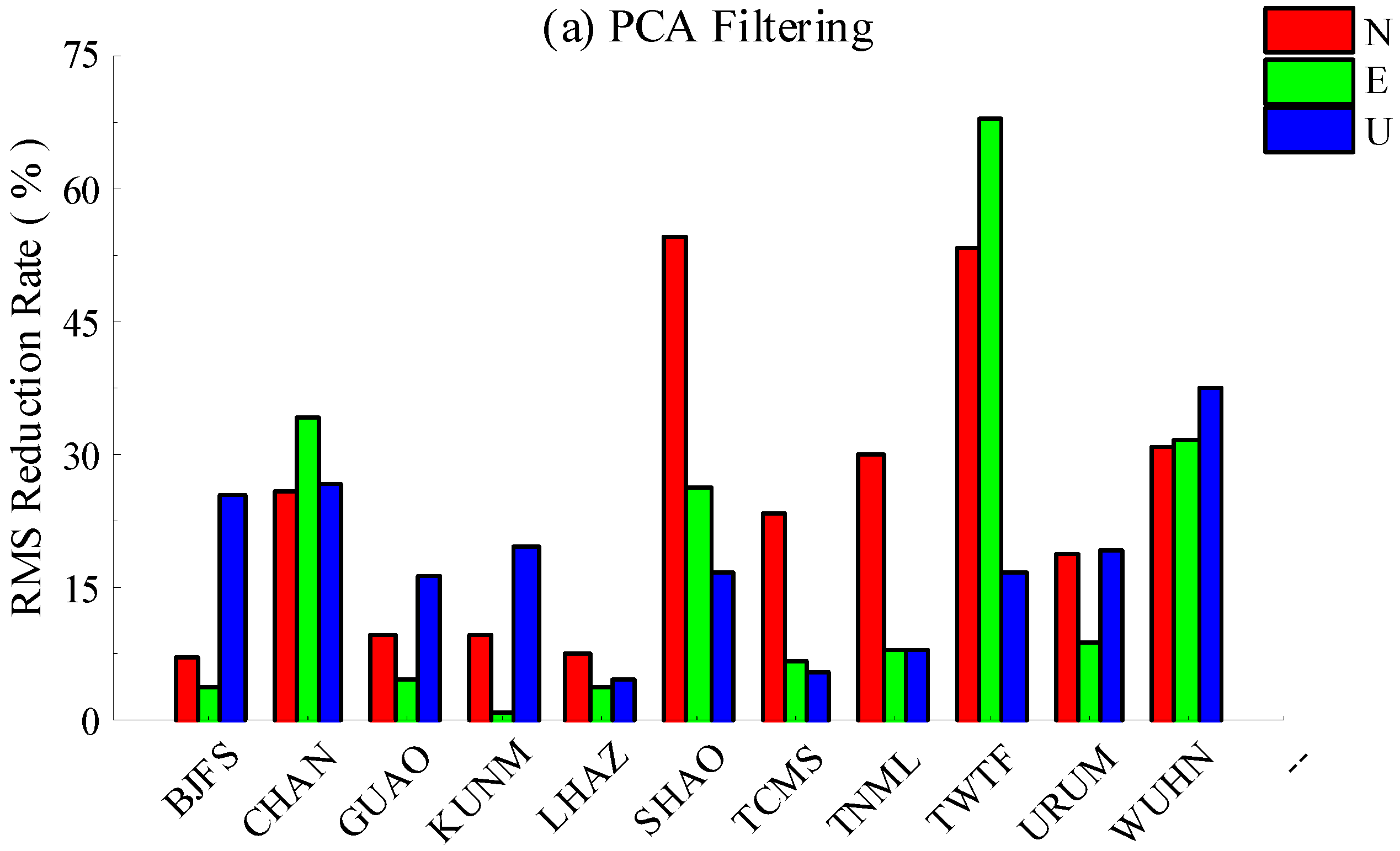
3.1. One Extraction from all IGS Stations
3.2. Influence of Region Size on CMC Extraction
3.3. Sub-Regional Extractions Considering Tectonic Units
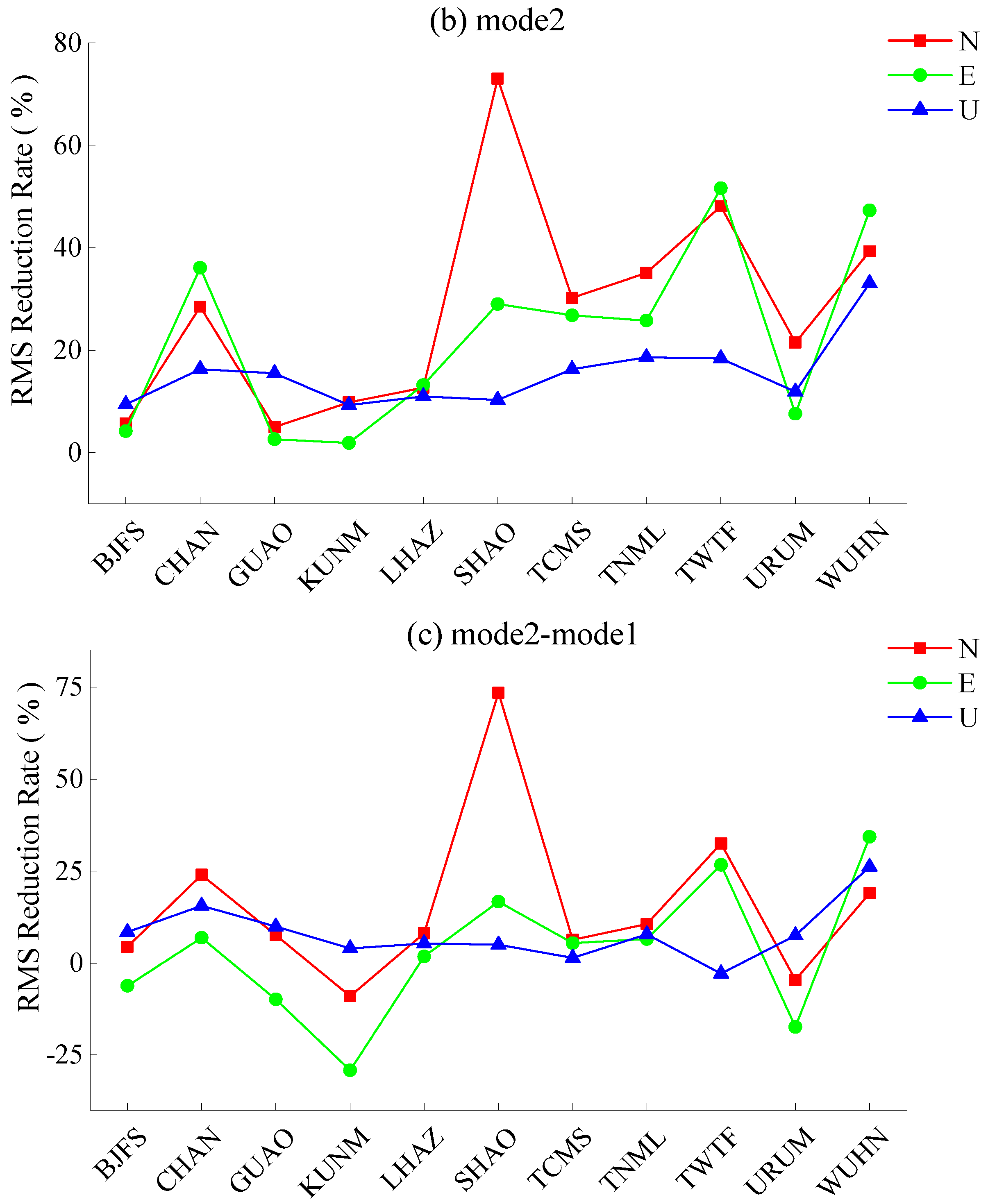
3.4. Comparison of Two CMC Extraction Modes
4. Relevant Geophysical Signals
5. Conclusions
- (1)
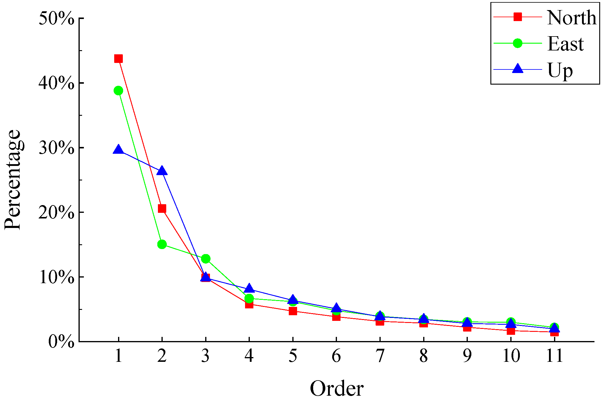
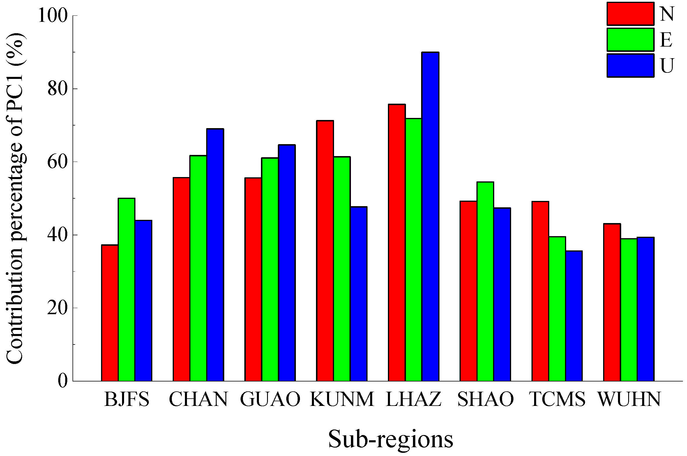
- The average PC1 contribution percentage of eight sub-regions in North, East and Up components are 54.6%, 54.9% and 54.7%, which increase by 10.8%, 16.1% and 25.1%, respectively, compared with the result of one whole region. The regional CMC extracted in sub-regional mode are more significant, and RMS reduction rates on more coordinate components are positive values after CMC extraction. Moreover, the differences of RMS reduction rates are positive on 78.8% coordinate components, indicating that PCA filtering in a sub-regional mode is a more effective filtering method for most coordinate components. This will help to improve SNR in GPS coordinate time series, and thus to reveal the surface deformation characteristics of the IGS station more realistically and accurately.
- (2)
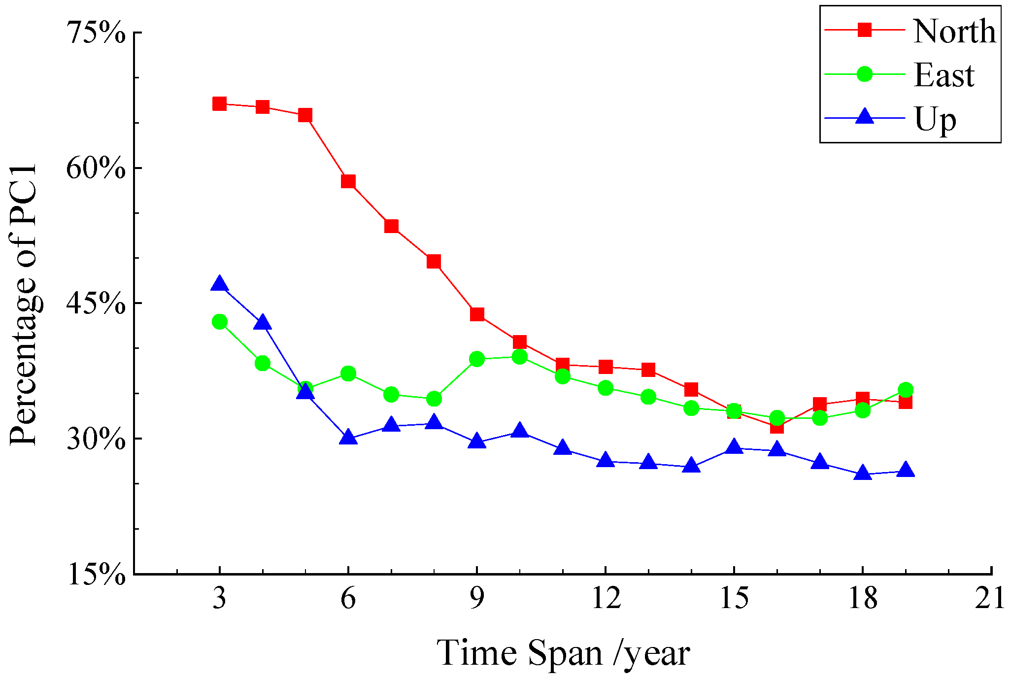
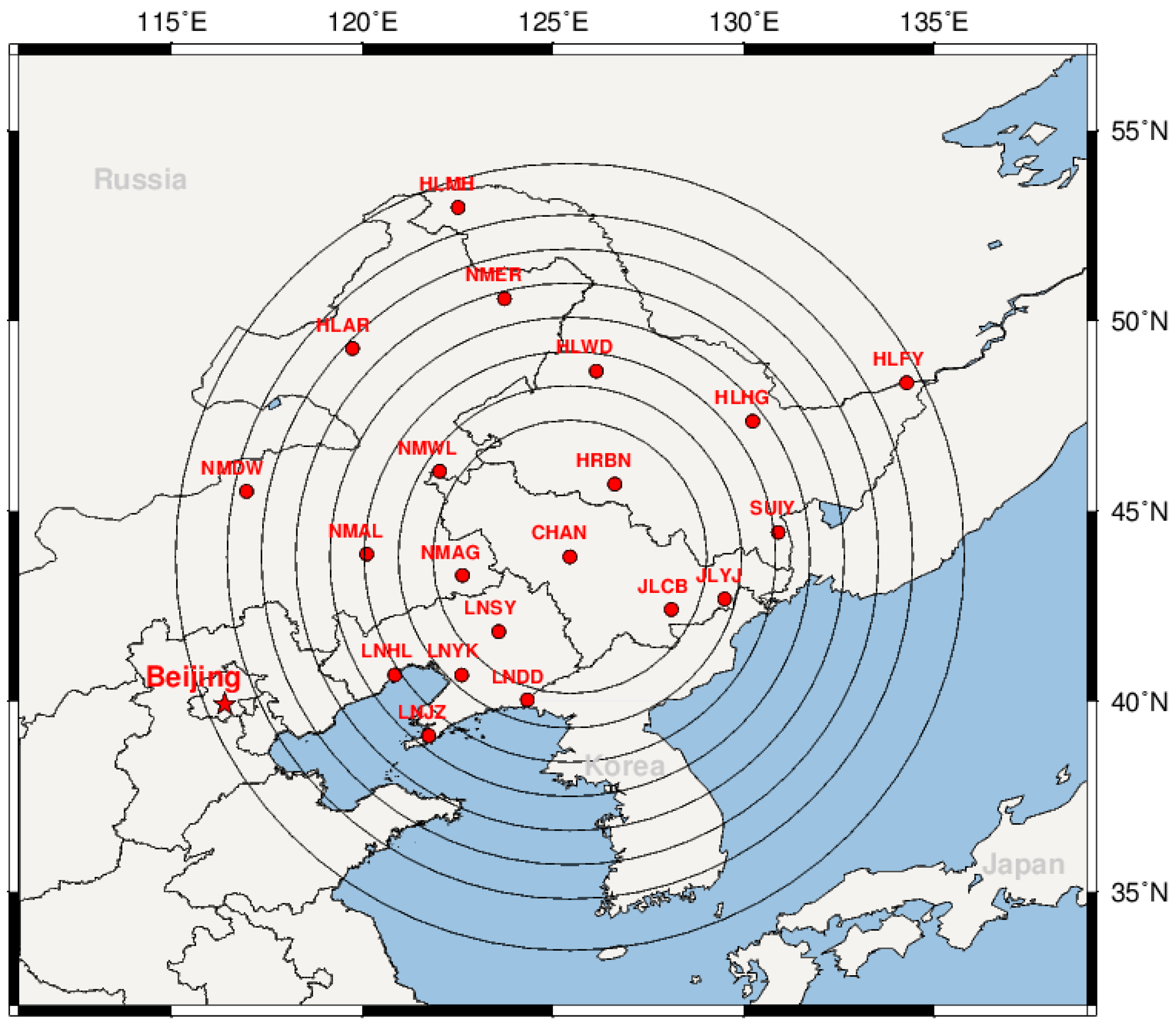
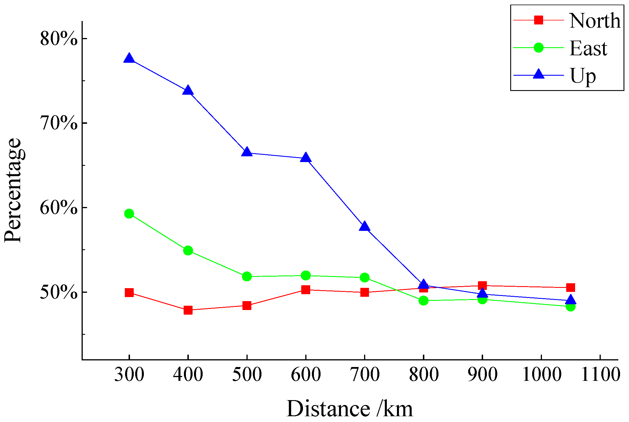
- Regional CMC is a spatiotemporal-dependent displacement series. It is affected by factors, such as the region size and time span of the coordinate time series. When the CMC of the IGS station in China is uniformly extracted, the length of the coordinate time series is inversely proportional to the percentage of PC1. The longer the time span is, the smaller the percentage of PC1. When the time series span is greater than 10 years, the percentage of PC1 in North and East components are about 34%, and about 26% in the Up component. In the Northeast Block of China, regional CMC of GPS stations can be extracted satisfactorily within the interstation distance of 600 km. The contribution percentages of PC1 in North, East and Up components are all over 50%, and along with the increase of region size, it does not change significantly in horizontal components but drops dramatically in the vertical direction.
- (3)
- This paper puts forward new criteria for selecting appropriate CMONOC stations near IGS stations when computing sub-regional CMC, including considerations of interstation distance, geology and self-condition of stations. Experimental results show that these criteria are implemental and effective in selecting suitable stations. PCA filtering with the above-mentioned criteria helps to improve the accuracy of coordinate time series of GPS stations, which is beneficial to reveal the deformation of the Earth surface.
- (4)
- PCA filtering and environmental loading corrections are two commonly used methods for analyzing non-linear variations of GPS coordinate time series. By comparison, we know that PCA filtering in sub-regional mode results in dramatic improvements of SNR in GPS coordinate time series. After ELCs, however, there are still 30.3% of the coordinate components with larger RMS reduction rates, probably because of the phase differences of the periodic terms between GPS coordinate time series and environmental loading displacements in the vertical components. Therefore, PCA filtering in sub-regional mode is superior to ELCs in improving the SNR of the GPS coordinate time series.
Author Contributions
Funding
Acknowledgments
Conflicts of Interest
References
- Jiang, Z.S.; Liu, J.N. The method in establishing strain field and velocity field of crustal movement using least squares collocation. Chin. J. Geophys. 2010, 53, 380–389, (in Chinese with English abstract). [Google Scholar] [CrossRef]
- Liang, S.M.; Gan, W.J.; Shen, C.Z.; Xiao, G.R.; Liu, J.; Chen, W.T.; Ding, X.G.; Zhou, D.M. Three-dimensional velocity field of present-day crustal motion of the Tibetan Plateau derived from GPS measurements. J. Geophys. Res. Solid Earth 2013, 118, 5722–5732. [Google Scholar] [CrossRef]
- Kreemer, C.; Blewitt, G.; Klein, E.C. A geodetic plate motion and Global Strain Rate Model. Geochem. Geophys. Geosyst. 2014, 15, 3849–3889. [Google Scholar] [CrossRef]
- Wang, W.; Qiao, X.J.; Yang, S.M.; Wang, D.J. Present-day velocity field and block kinematics of Tibetan Plateau from GPS measurements. Geophys. J. Int. 2017, 208, 1088–1102. [Google Scholar] [CrossRef]
- Klos, A.; Gruszczynska, M.; Bos, M.; Boy, J.; Bogusz, J. Estimates of Vertical Velocity Errors for IGS ITRF2014 Stations by Applying the Improved Singular Spectrum Analysis Method and Environmental Loading Models. Pure Appl. Geophys. 2018, 175, 1823–1840. [Google Scholar] [CrossRef]
- Yuan, P.; Jiang, W.P.; Wang, K.H.; Sneeuw, N. Effects of Spatiotemporal Filtering on the Periodic Signals and Noise in the GPS Position Time Series of the Crustal Movement Observation Network of China. Remote Sens. 2018, 10, 1472. [Google Scholar] [CrossRef]
- Wdowinski, S.; Bock, Y.; Zhang, J.; Fang, P.; Genrich, J. Southern California permanent GPS geodetic array: Spatial filtering of daily positions for estimating coseismic and postseismic displacement induced by the 1992 Landers earthquake. J. Geophys. Res. Solid Earth 1997, 102, 18057–18070. [Google Scholar] [CrossRef]
- Johansson, J.M.; Davis, J.L.; Scherneck, H.G.; Milne, G.A.; Vermeer, M.; Mitrovica, J.X.; Bennett, R.A.; Jonsson, B.; Elgered, G.; Elósegui, P.; et al. Continuous GPS measurements of postglacial adjustment in Fennoscandia-1. Geodetic results. J. Geophys. Res. Solid Earth 2002, 107, ETG 3-1–ETG 3-27. [Google Scholar] [CrossRef]
- Dong, D.; Fang, P.; Bock, Y.; Webb, F.; Prawirodirdjo, L.; Kedar, S.; Jamason, P. Spatiotemporal filtering using principal component analysis and Karhunen—Loeve expansion approaches for regional GPS network analysis. J. Geophys. Res. Solid Earth 2006, 111, 1581–1600. [Google Scholar] [CrossRef]
- Yuan, L.; Ding, X.; Chen, W.; Guo, Z.H.; Chen, S.B.; Hong, B.S.; Zhou, J.T. Characteristics of daily position time series from the Hong Kong GPS fiducial network. Chin. J. Geophys. 2008, 51, 1372–1384, (in Chinese with English abstract). [Google Scholar] [CrossRef]
- Márquez-Azúa, B.; DeMets, C. Crustal velocity field of Mexico from continuous GPS measurements, 1993 to June 2001: Implications for the neotectonics of Mexico. J. Geophys. Res. Solid Earth 2003, 108, 149–169. [Google Scholar] [CrossRef]
- Serpelloni, E.; Faccenna, C.; Spada, G.; Dong, D.; Williams, S.D.P. Vertical GPS ground motion rates in the Euro-Mediterranean region: New evidence of velocity gradients at different spatial scales along the Nubia-Eurasia plate boundary. J. Geophys. Res. Solid Earth 2013, 118, 6003–6024. [Google Scholar] [CrossRef] [Green Version]
- Shen, Y.Z.; Li, W.W.; Xu, G.C.; Li, B.F. Spatiotemporal filtering of regional GNSS network’s position time series with missing data using principle component analysis. J. Geod. 2014, 88, 1–12. [Google Scholar] [CrossRef]
- He, X.X.; Hua, X.H.; Yu, K.G.; Xuan, W.; Lu, T.D.; Zhang, W.; Chen, X. Accuracy enhancement of GPS time series using principal component analysis and block spatial filtering. Adv. Space Res. 2015, 60, 1316–1327. [Google Scholar] [CrossRef]
- Tian, Y.F.; Shen, Z.K. Extracting the regional common-mode component of GPS station position time series from dense continuous network. J. Geophys. Res. Solid Earth 2016, 121, 1080–1096. [Google Scholar] [CrossRef]
- Ma, C.; Li, F.; Zhang, S.K.; Lei, J.T.; E, D.C.; Hao, W.F.; Zhang, Q.C. The coordinate time series analysis of continuous GPS stations in the Antarctic Peninsula with consideration of common mode error. Chin. J. Geophys. 2016, 59, 2783–2795, (in Chinese with English abstract). [Google Scholar]
- Ming, F.; Yang, Y.X.; Zeng, A.M.; Zhao, B. Spatiotemporal filtering for regional GPS network in China using independent component analysis. J. Geod. 2017, 91, 419–440. [Google Scholar] [CrossRef]
- Zhu, Z.H.; Zhou, X.H.; Deng, L.S.; Wang, K.H.; Zhou, B.Y. Quantitative Analysis of Geophysical Sources of Common Mode Component in CMONOC GPS Coordinate Time Series. Adv. Space Res. 2017, 60, 2896–2909. [Google Scholar] [CrossRef]
- Yuan, P.; Li, Z.; Jiang, W.P.; Ma, Y.F.; Chen, W.; Sneeuw, N. Influences of Environmental Loading Corrections on the Nonlinear Variations and Velocity Uncertainties for the Reprocessed Global Positioning System Height Time Series of the Crustal Movement Observation Network of China. Remote Sens. 2018, 10, 958. [Google Scholar] [CrossRef]
- Jiang, Z.H.; Zhang, P.; Bei, J.Z.; Liu, L.F. Velocity estimation on the colored noise properties of CORS network in China based on the CGCS2000 frame. Acta Geod. Cartogr. Sin. 2010, 39, 355–363, (in Chinese with English abstract). [Google Scholar]
- Williams, S.D.P.; Bock, Y.; Fang, P.; Jamason, P.; Nikolaidis, R.M.; Prawirodirdjo, L.; Miller, M.; Johnson, D.J. Error analysis of continuous GPS position time series. J. Geophys. Res. 2004, 109, B03412. [Google Scholar] [CrossRef]
- Tian, Y.F. Study on Intermediate- and long-term Errors in GPS Position Time Series. Ph.D. Thesis, Institute of Geology, China Earthquake Administration, Beijing, China, 2011. [Google Scholar]
- Farrell, W.E. Deformation of the Earth by surface loads. Rev. Geophys. 1972, 10, 761–797. [Google Scholar] [CrossRef]
- Van Dam, T.; Wahr, J.M. Displacements of the Earth’s surface due to atmospheric loading: Effects on gravity and baseline measurements. J. Geophys. Res. Solid Earth 1987, 92, 1281–1286. [Google Scholar] [CrossRef]
- Van Dam, T.; Böhm, J. Loading Effects and Reference Frames. In Encyclopedia of Geodesy; Grafarend, E., Ed.; Springer: Basel, Switzerland, 2016; pp. 1–5. ISBN 978-3-319-02370-0. [Google Scholar]
- Dill, R.; Dobslaw, H. Numerical simulations of global-scale high-resolution hydrological crustal deformations. J. Geophys. Res. Solid Earth 2013, 118, 5008–5017. [Google Scholar] [CrossRef]
- Marsland, S.J.; Haak, H.; Jungclaus, J.H.; Latif, M.; Röske, F. The Max-Planck-Institute global ocean/sea ice model with orthogonal curvilinear coordinates. Ocean Model. 2003, 5, 91–127. [Google Scholar] [CrossRef] [Green Version]
- Dill, R. Hydrological Model LSDM for Operational Earth Rotation and Gravity Field Variations; Scientific Technical Report STR08/09; GFZ: Potsdam, Germany, 2008. [Google Scholar]
- Blewitt, G. Self-consistency in reference frames, geocenter definition, and surface loading of the solid Earth. J. Geophys. Res. Solid Earth 2003, 108, B2. [Google Scholar] [CrossRef]
- Jiang, W.P.; Xia, C.Y.; Li, Z.; Guo, Q.Y.; Zhang, S.Q. Analysis of environmental loading effects on regional GPS coordinate time series. Acta Geod. Cartogr. Sin. 2014, 43, 1217–1223, (in Chinese with English abstract). [Google Scholar]
- Li, F.; Ma, C.; Zhang, S.K.; Lei, J.T.; Hao, W.F.; Zhang, Q.C.; Li, W.H. Noise analysis of the coordinate time series of the continuous GPS stations and deformation patterns in the Antarctic Peninsula. Chin. J. Geophys. 2016, 59, 2402–2412, (in Chinese with English abstract). [Google Scholar]
- Jackson, D.A.; Chen, Y. Robust principal component analysis and outlier detection with ecological data. Environmetrics 2004, 15, 129–139. [Google Scholar] [CrossRef]
- Bevis, M.; Brown, A. Trajectory models and reference frames for crustal motion geodesy. J. Geod. 2014, 88, 283–311. [Google Scholar] [CrossRef] [Green Version]
- Nikolaidis, R. Observation of Geodetic and Seismic Deformation with the Global Positioning System. Ph.D. Thesis, University of California, San Diego, CA, USA, 2002. [Google Scholar]
- Gazeaux, J. Detecting offsets in GPS time series: First results from the detection of offsets in GPS experiment. J. Geophys. Res. Solid Earth 2013, 118, 2397–2407. [Google Scholar] [CrossRef] [Green Version]
- Wang, X.Y.; Zhu, W.Y.; Fu, Y.; You, Z.X.; Wang, Q.; Cheng, Z.Y.; Ren, J.W. Present-time crustal deformation in China and surrounding regions by GPS. Chin. J. Geophys. 2002, 45, 198–209, (in Chinese with English abstract). [Google Scholar] [CrossRef]
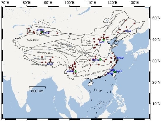
- Liu, X.; Li, T.D.; Geng, S.F.; You, G.Q. Geotectonic division of China and some related problems. Geol. Bull. China 2012, 31, 1024–1034, (in Chinese with English abstract). [Google Scholar]
- Liu, X.; You, G.Q. Tectonic regional subdivision of China in the light of plate theory. Geol. China 2015, 42, 1–17, (in Chinese with English abstract). [Google Scholar]
- Jiang, W.P.; Li, Z.; Liu, H.F.; Zhao, Q. Cause analysis of the non-linear variation of the IGS reference station coordinate time series inside China. Chin. J. Geophys. 2013, 56, 2228–2237, (in Chinese with English abstract). [Google Scholar]


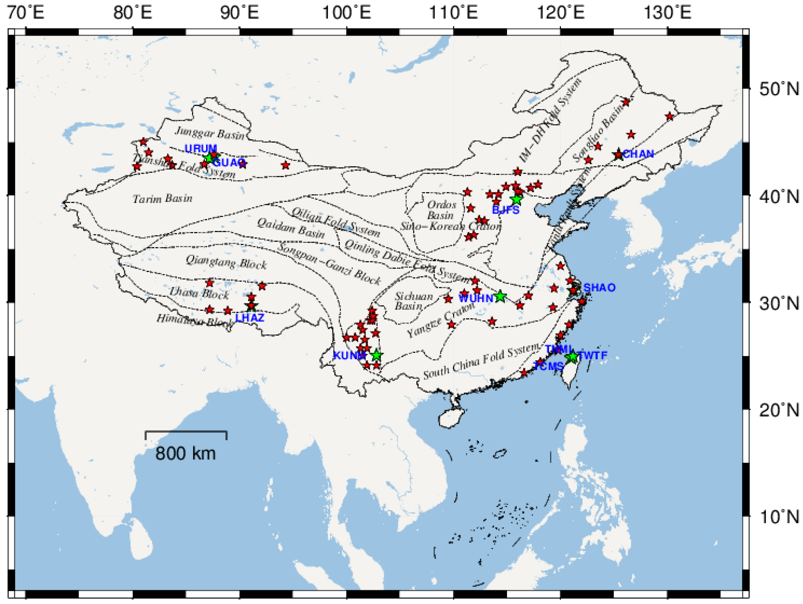
| Station | Latitude/° | Longitude/° | Session/year | Time Span/Year | Monument/Bedrock Type |
|---|---|---|---|---|---|
| BJFS | 39.60861 | 115.89222 | 1999.8041–2018.8945 | 19.1 | concrete/weathered sedimentary |
| CHAN | 43.79050 | 125.44330 | 2004.9385–2018.8973 | 14.0 | concrete/weathered sedimentary |
| GUAO | 43.47110 | 87.17730 | 2002.4534–2016.2008 | 13.7 | reinforced concrete/metamorphic |
| URUM | 43.59000 | 87.63000 | 1998.7685–2013.0836 | 14.3 | concrete/bedrock |
| KUNM | 25.02950 | 102.79720 | 1999.7247–2018.8973 | 19.2 | concrete/sedimentary |
| LHAZ | 29.65722 | 91.10389 | 1995.0233–2018.8973 | 23.9 | roof concrete/none |
| SHAO | 31.09944 | 121.20028 | 2002.4781–2018.8808 | 16.4 | concrete/sedimentary |
| TCMS | 24.79778 | 120.98722 | 2002.4781–2018.8699 | 16.4 | roof steel/sedimentary |
| TNML | 24.79800 | 120.98730 | 2001.8562–2018.8945 | 17.0 | roof steel/sedimentary |
| TWTF | 24.95360 | 121.16450 | 1998.8342–2018.8945 | 20.1 | roof steel/none |
| WHUN | 30.53139 | 114.35722 | 1996.0669–2016.7363 | 20.7 | granite block/sedimentary |
| Station | North | East | Up | ||||||
|---|---|---|---|---|---|---|---|---|---|
| p1 | p2 | p3 | p1 | p2 | p3 | p1 | p2 | p3 | |
| BJFS | −0.16 | 0.90 | 0.32 | 0.73 | −0.35 | 0.63 | 1.00 | −0.11 | −0.26 |
| CHAN | −0.12 | 1.00 | −0.22 | 0.86 | −0.33 | −0.06 | 0.70 | −0.02 | −0.08 |
| GUAO | −0.03 | 0.63 | 1.00 | 0.78 | −0.61 | −0.40 | 0.49 | −0.19 | 1.00 |
| KUNM | 0.56 | −0.21 | 0.93 | 0.76 | −0.86 | −0.10 | 0.84 | −0.61 | −0.20 |
| LHAZ | 0.16 | 0.92 | 0.60 | 0.80 | −0.40 | −0.15 | 0.65 | 0.07 | 0.80 |
| URUM | 0.88 | −0.47 | 0.30 | 0.50 | 0.05 | 1.00 | 0.81 | −0.29 | −0.34 |
| SHAO | 0.83 | 0.53 | −0.58 | 1.00 | 1.00 | −0.29 | 0.77 | 0.92 | −0.30 |
| TCMS | 0.82 | 0.40 | −0.65 | 0.96 | 0.97 | −0.34 | 0.76 | 0.80 | −0.21 |
| TNML | 1.00 | −0.14 | −0.07 | 0.54 | 0.20 | 0.22 | 0.05 | 1.00 | 0.33 |
| TWTF | −0.26 | 0.89 | −0.48 | 0.95 | −0.47 | −0.28 | 0.53 | −0.84 | 0.00 |
| WUHN | 0.73 | 0.37 | 0.18 | 0.84 | 0.43 | 0.45 | 0.73 | −0.02 | 0.16 |
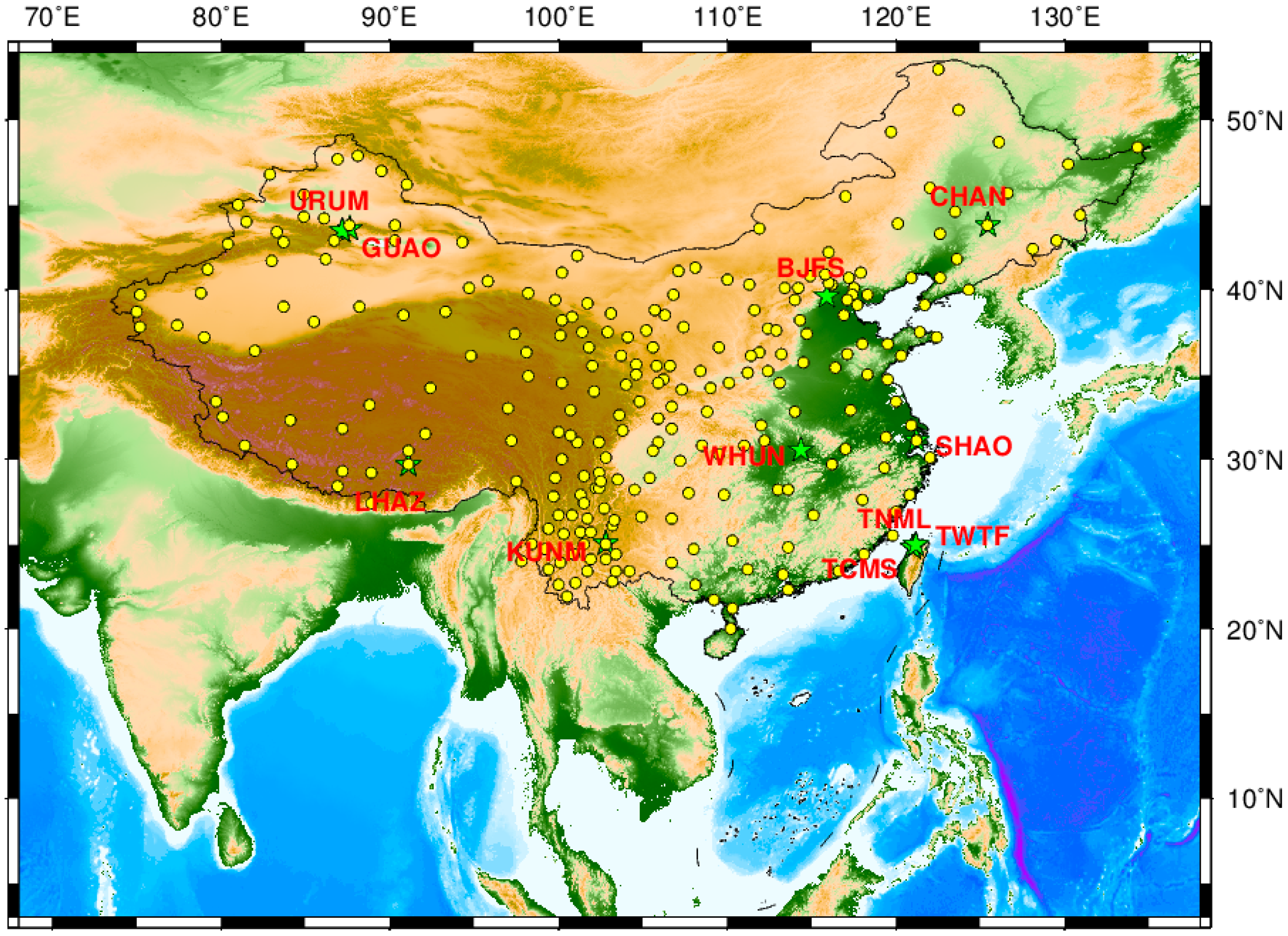
| Station | Latitude/° | Longitude/° | Session/Year | Distance Away to CHAN/km | Monument Type |
|---|---|---|---|---|---|
| CHAN | 43.79069 | 125.44420 | 2004.9385–2018.9822 | 0 | bedrock |
| HRBN | 45.70261 | 126.62037 | 2003.0014–2018.9959 | 231.973 | soil |
| NMAG | 43.30348 | 122.62722 | 2010.4973–2018.9959 | 233.983 | bedrock |
| JLCB | 42.41055 | 128.10593 | 2010.6233–2018.9959 | 265.425 | bedrock |
| LNSY | 41.82708 | 123.57948 | 2010.5849–2018.9959 | 266.143 | soil |
| JLYJ | 42.68296 | 129.50451 | 2011.1959–2018.9959 | 344.581 | soil |
| NMWL | 46.04064 | 122.02728 | 2011.0068–2018.9959 | 367.755 | bedrock |
| LNYK | 40.68354 | 122.60304 | 2010.5685–2018.9959 | 417.151 | bedrock |
| LNDD | 40.03162 | 124.32725 | 2010.6068–2018.9959 | 427.606 | bedrock |
| NMAL | 43.86335 | 120.11291 | 2010.7877−2018.9959 | 428.789 | bedrock |
| SUIY | 44.43334 | 130.90807 | 1999.1630−2018.9959 | 443.044 | granodiorite |
| LNHL | 40.68769 | 120.85180 | 2010.8178−2018.9959 | 512.057 | bedrock |
| HLHG | 47.35276 | 130.23563 | 2011.0041−2018.9959 | 544.274 | bedrock |
| HLWD | 48.67141 | 126.13617 | 2010.6041−2018.9959 | 544.990 | bedrock |
| LNJZ | 39.09181 | 121.74011 | 2011.0041−2018.9959 | 606.403 | bedrock |
| NMDW | 45.51310 | 116.96303 | 2010.6041−2018.9959 | 698.775 | bedrock |
| HLAR | 49.27049 | 119.74126 | 2010.4973−2018.9959 | 749.134 | bedrock |
| NMER | 50.57642 | 123.72720 | 1999.1630−2018.9959 | 765.064 | andesite |
| HLFY | 48.36699 | 134.27715 | 2010.6507−2018.9959 | 850.307 | bedrock |
| HLMH | 52.97508 | 122.51272 | 2011.0151−2018.9959 | 1042.765 | bedrock |
| Station | Location | Second-Class Tectonic Units | Number of Near CMONOC Stations | The Farthest CMONOC Station/Distance |
|---|---|---|---|---|
| BJFS | Beijing | North China Block (craton) | 16 | SXLF/558 km |
| CHAN | Changchun | Songliao Basin | 7 | HLWD/545 km |
| GUAO | Urumchi | Tianshan Fold System | 9 | XJJJ/586 km |
| KUNM | Kunming | Sichuan-Yunnan Rhombic Block | 15 | SCSM/467 km |
| LHAZ | Lhasa | Lhasa Sub-block | 6 | XZNM/440 km |
| SHAO | Shanghai | Yangtze Block (craton) | 7 | JXHK/500 km |
| TCMS | Hsinchu | South China Orogenic Zone | 6 | ZJZS/592 km |
| TNML | Hsinchu | South China Orogenic Zone | 6 | ZJZS/592 km |
| TWTF | Taoyuan | South China Orogenic Zone | 6 | ZJZS/573 km |
| URUM | Urumchi | Tianshan Fold System | 9 | XJZS/600 km |
| WHUN | Wuhan | Yangtze Block (craton) | 7 | HNMY/532 km |
© 2019 by the authors. Licensee MDPI, Basel, Switzerland. This article is an open access article distributed under the terms and conditions of the Creative Commons Attribution (CC BY) license (http://creativecommons.org/licenses/by/4.0/).
Share and Cite
Wu, S.; Nie, G.; Liu, J.; Wang, K.; Xue, C.; Wang, J.; Li, H.; Peng, F.; Ren, X. A Sub-Regional Extraction Method of Common Mode Components from IGS and CMONOC Stations in China. Remote Sens. 2019, 11, 1389. https://0-doi-org.brum.beds.ac.uk/10.3390/rs11111389
Wu S, Nie G, Liu J, Wang K, Xue C, Wang J, Li H, Peng F, Ren X. A Sub-Regional Extraction Method of Common Mode Components from IGS and CMONOC Stations in China. Remote Sensing. 2019; 11(11):1389. https://0-doi-org.brum.beds.ac.uk/10.3390/rs11111389
Chicago/Turabian StyleWu, Shuguang, Guigen Nie, Jingnan Liu, Kezhi Wang, Changhu Xue, Jing Wang, Haiyang Li, Fengyou Peng, and Xiaobin Ren. 2019. "A Sub-Regional Extraction Method of Common Mode Components from IGS and CMONOC Stations in China" Remote Sensing 11, no. 11: 1389. https://0-doi-org.brum.beds.ac.uk/10.3390/rs11111389