Article

Automatic Updating of Land Cover Maps in Rapidly Urbanizing Regions by Relational Knowledge Transferring from GlobeLand30

1
School of Geography and Ocean Science, Nanjing University, Nanjing 210093, China
2
Key Laboratory for Satellite Mapping Technology and Application of National Administration of Surveying, Mapping and Geoinformation of China, Nanjing University, Nanjing 210093, China
3
Jiangsu Provincial Key Laboratory of Geographic Information Science and Technology, Nanjing University, Nanjing 210093, China
4
State Key Laboratory of Desert and Oasis Ecology, Xinjiang Institute of Ecology and Geography, Chinese Academy of Sciences, Ürümqi 830011, China
5
School of Geography, Geomatics and Planning, Jiangsu Normal University, Xuzhou 221116, China
6
Geoinformatics Unit, RIKEN Center for Advanced Intelligence Project, Tokyo 103-0027, Japan
*
Author to whom correspondence should be addressed.
Remote Sens. 2019, 11(12), 1397; https://0-doi-org.brum.beds.ac.uk/10.3390/rs11121397
Submission received: 30 April 2019 / Revised: 29 May 2019 / Accepted: 5 June 2019 / Published: 12 June 2019
(This article belongs to the Special Issue Operational Land Cover/Land Use Mapping)

Abstract

:
Land-cover map is the basis of research and application related to urban planning, environmental management and ecological protection. Land-cover updating is an essential task especially in a rapidly urbanizing region, where fast development makes it necessary to monitor land-cover change in a timely manner. However, conventional approaches always have the limitations of large amounts of sample collection and exploitation of relational knowledge between multi-modality remote sensing datasets. With some global land-cover products being available, it is important to produce new land-cover maps based on the existing land-cover products and time series images. To this end, a novel transfer learning based automatic approach was proposed for updating land cover maps of rapidly urbanizing regions. In detail, the proposed method is composed of the following three steps. The first is to design a strategy to extract reliable land-cover information from the historical land-cover map for one of the images (source domain). Then, a novel relational knowledge transfer technique is applied to transfer label information. Finally, classifiers are trained on the transferred samples with spatio-spectral features. The experimental results show that aforementioned steps can select sufficient effective samples for target images, and for the main land-cover classes in a rapidly urbanizing region; the results of an updated map show good performance in both precision and vision. Therefore, the proposed approach provides an automatic solution for urban land-cover mapping with a high degree of accuracy.

Graphical Abstract

1. Introduction

Over past decades, rapid population growth and urbanization have taken place at an unprecedented rate all over the world. For instance, more than half of the world’s population lived in urban areas in 2008, and this figure is projected to rise to 70% by 2050, with most of the growth occurring in developing countries [1,2]. Urbanization, as an important landscape pattern change process, is rapidly transforming natural land-cover to anthropogenic urban land use [3]. However, the rapid urbanization process leads to a series of environment and development problems (e.g., deforestation [4], agriculture land loss [5], air pollution [6], and urban heat island effect [7]). Therefore, it is of crucial importance to understand the trends in urban sprawl and detect land-cover change [8], particularly in rapidly urbanizing regions, for urban planning and environment sustainability.
Satellite remote sensing, such as Moderate Resolution Imaging Spectroradiometer (MODIS) observation [9], Landsat observation [10,11,12] and Sentinel observation [13], has been used to urban land-cover mapping at different scales. With the development of remote sensing image processing; land-cover datasets produced from satellite images have been widely used in the earth surface processes modeling, sustainable development planning and so on. Several global land-cover products have arisen with efforts of international scientific organizations during the past decades [14,15]. Most of them derived by using satellite images at 300–1000 m spatial resolution, such as University of Maryland land-cover dataset (UMD) [16], MODIS land-cover product (MOD12Q1 and MCD12Q1) [17] and Climate Change Initiative land-cover product (CCL-LC) from European space agency (ESA), did not provide sufficient thematic detail or change information [14], especially in urban areas. More recent research focused on the global urban mapping aim to provide spatially more accurate urban thematic layers based on finer resolution satellite images. A multiscale high-resolution image process framework for supporting Global Human Settlement Layer (GHSL) was presented in [18] with the operational test result involved in the mapping of 24.3 million km2 of urban areas. The Urban Footprint Processor (UFP) [19], which is a fully automated method for the delineation of human settlements by the SAR data, was used to produce a new global urban dataset called the Global Urban Footprint (GUF) raster map [20]. In order to overcome spectral confusion between urban and nonurban land-cover classes, a hierarchical object-based texture (HOTex) was developed and applied to produce a new global map of built-up and settlement extent [21]. It is worth mentioning that GlobeLand30 land-cover product, with improved spatial resolution and accuracy, has been developed by the National Geomatics Center of China [10,22]. This 30 m product is based on Landsat and similar satellite images, which allows it to support the updating and reconstruction of land-cover maps due to the continuous observation of Landsat. Since many of these products presented land-cover map at a few static time instants, their timeliness is far from satisfactory for many applications in urban areas. Accurate and timely information about land-cover change is vital to the comprehension and management of urbanization dynamics [23].
Most of the current approaches update land-cover maps based on the supervised classification that always requires large amounts of samples. The generation of training samples is a time-intensive, expensive, and subjective task. Therefore, a sufficient number of training samples for operational land-cover mapping is not always feasible due to the high cost and time-consuming process [24,25,26]. Several training data automation methods were proposed as an alternative to manual selection. For example, Training Data Automation (TDA) methods for forest cover mapping and built-up area extraction were designed in [27] and [28], respectively. An automatic approach was proposed in [29] to classify vegetation, water and impervious surface areas, and bare land with training data automation procedure based on several spectral indices. However, most of the current TDA methods focused on several specific land-cover type, and some important land-cover types were not considered (e.g., cultivated land and wetland). When the training dataset is selected from an image that is different from the one used for classification; spectral shifts between the two distributions are likely to make the classification model fail. Such shifts due to differences in acquisition and atmospheric conditions or to the changes in landscape are defined as data-shift problems [30]. Especially, in land cover map updating, using time series images scenario cases where the data-shift problem is always inevasible. Thus, developing a method capable of exploitation of relational knowledge between existing land-cover products and time series images is appealing for automatic updating large-scale land-cover maps.
To solve the data-shift problems that exist in multi-temporal and multi-modality remote sensing imageries; plenty of approaches have been proposed in the last decades. Popular solutions including: absolute and relative image normalization [31], histogram matching [32], Principal Component Analysis (PCA) [33] and Tasselled Cap (TC) [34] transformation. In contrast with above and other conventional solutions, the Transfer Learning (TL) approach has gained increasing attention in recent years. TL is defined as follows [35]: given data and the learning task of source domain, data and learning task of target domain, transfer learning aims to help improve the learning of the target predictive function in target domain using the knowledge in source domain and its learning task. Domain Adaptation (DA) is a particular form of TL. These two domains in remote sensing communities are associated with two satellite images acquired on different areas or on the same area at a different time. TL techniques aim to adapt the priori information of source domain to train a classifier used to predict the label in the target domain for the purpose of classification [30]. To this end, a widely used approach is based on adaptation of classifier with source domain samples and labeled/unlabeled target-domain samples. In this approach, training samples from source domain are used for initializing the learning task and the data of target domain is applied to adapting the model by a series of methods and strategies, such as Domain Adaptation Support Vector Machine (DASVM) [36], Active Learning (AL) technique [37], Change-Detection-driven Transfer Learning (CDTL) [38], Geodesic Flow Kernel Support Vector Machine (GFKSVM) [39] and iterative source samples reweighting strategy [40]. Another popular approach focuses on searching a shared and invariant feature subset. The main idea of this approach is to find an appropriate subspace by feature selection methods, such as Transfer Component Analysis (TCA) [41] and Manifold Alignment (MA) [42].
According to relevant remote sensing literatures [30,40,43], TL approaches are usually summarized into four categories, which are instance transfer, parameter transfer, feature representation transfer and relational knowledge transfer. Relational knowledge transfer approaches reuse the knowledge acquired in source domain to solve the learning problem in a related target domain [43]. The land-cover products, such as Globeland30, provide land-cover knowledge with sufficient sample labels. Considering that Globeland30 is produced mainly based on Landsat images, Globeland30 and its corresponding Landsat image can be defined as source domain, and other Landsat images acquired on the same geographical area can be defined as the target domain. The land-cover maps of target domain can be updated by a relational knowledge transfer approach, theoretically. Based on this idea, a new automatic updating approach was explored to customize a methodology to rapidly urbanizing regions. The method was designed to leverage multi-modality remote sensing dataset, capture high-quality sample labels from land-cover product, and derive the updated land-cover map by unsupervised knowledge transfer procedure. In addition, a novel sample selection strategy is designed as an alternative to traditional random selection method.
The paper is organized as follows: Section 2 introduces study areas and data sources; 
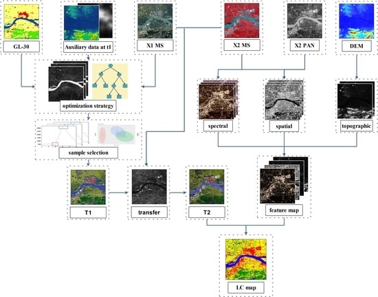
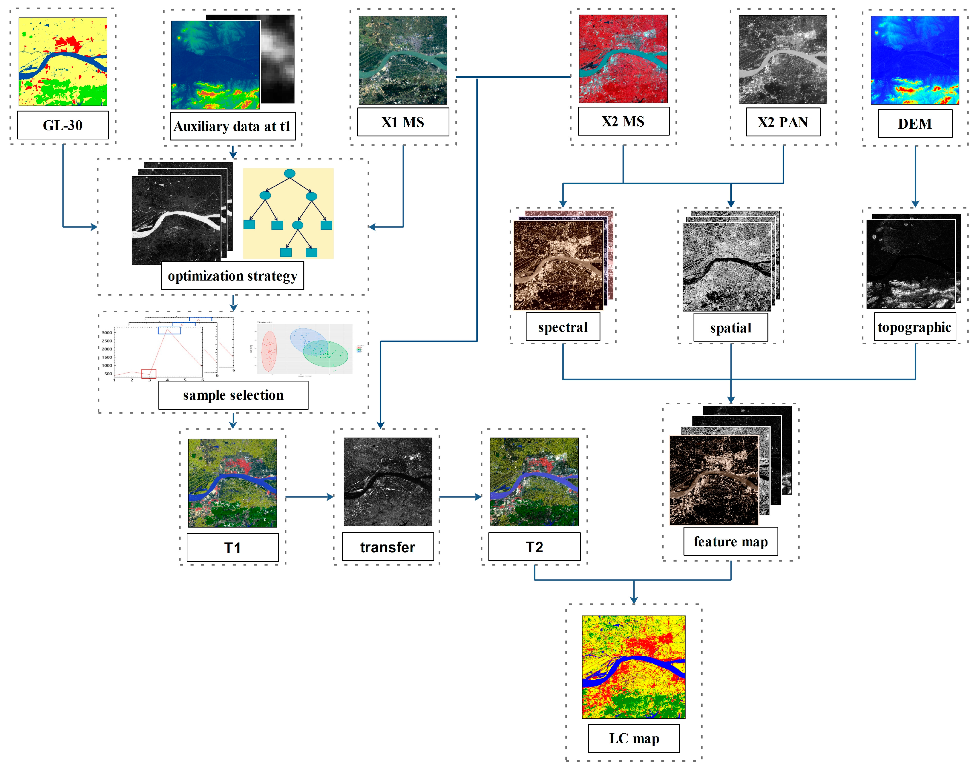
Section 3 introduces the workflow of the proposed approach; Section 4 evaluates the model performance with reference data. Finally, Section 5 concludes this paper.

2. Study Areas and Materials

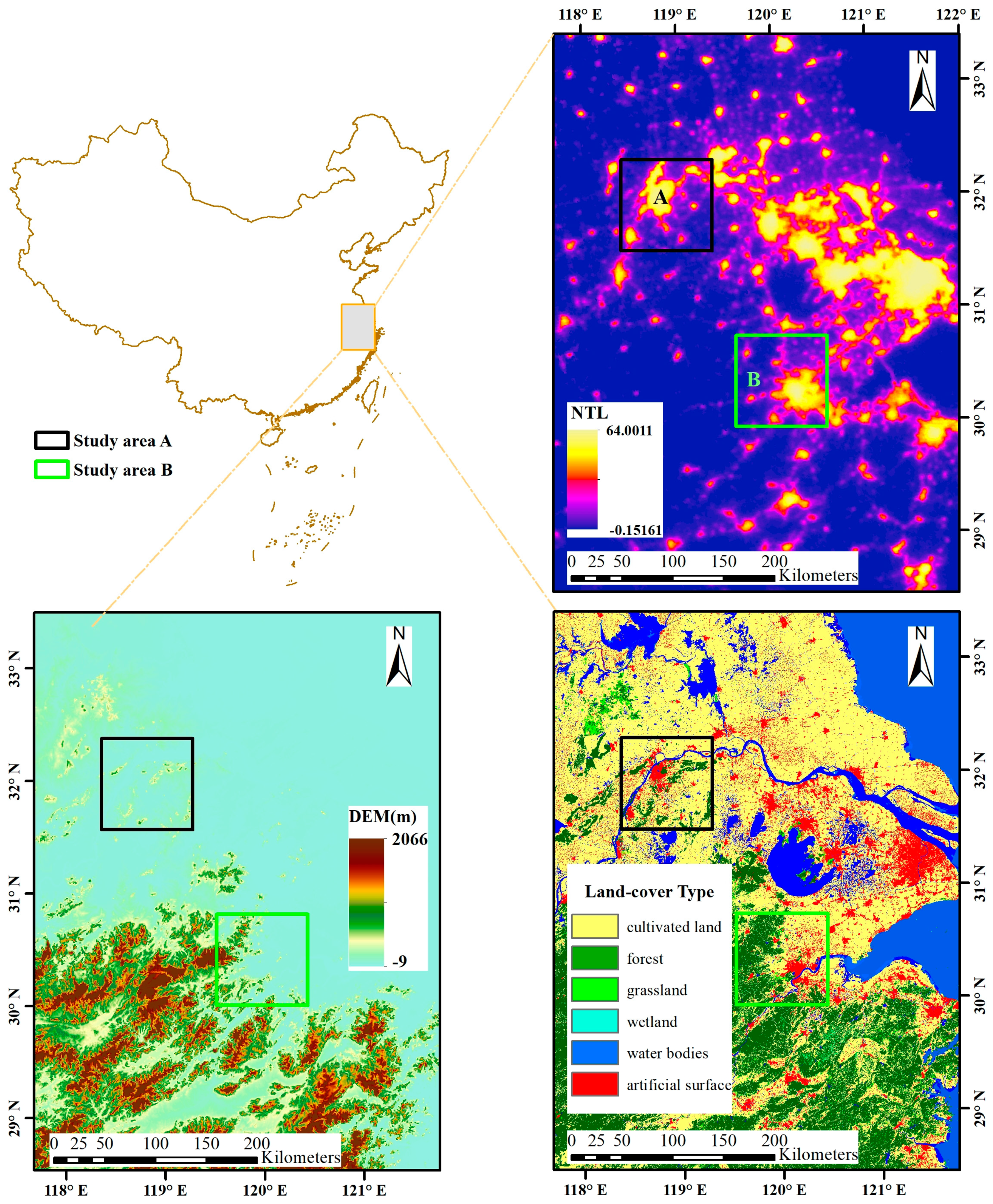
Two cities within the Yangtze River Delta city cluster were selected to update land-cover maps (Figure 1). One of them is the urban area of Nanjing and its surrounding areas, and the other is the urban area of Hangzhou and its surrounding areas. Each study area has an area of 8100 km2. Nanjing is the capital of the Jiangsu province and the second largest city in the East China region. Hangzhou is the capital and most populous city of the Zhejiang Province and it sits at the head of Hangzhou Bay, which separates Shanghai and Ningbo. Both Nanjing and Hangzhou are important economic hubs of the Yangtze River Delta city cluster, which is planned to build a world-class city cluster. In recent years, land-cover in these two regions has changed rapidly under the influence of urban expansion.
The nighttime light (NTL) data was obtained from version 4 of the DMSP/OLS NTL cloud-free annual composites. These data were observed by six satellites spanning over 22 years from 1992 to 2013. The main dataset used in this paper is the average stable light with a spatial resolution of 30 arc seconds. The average stable light product containing lights from human active areas with continuous nighttime light has demonstrated potential for mapping or monitoring urban area [23,44]. We chose this product to separate the artificial surface from other land-cover types. In order to obtain quality-enhanced NTL data, the original DN value was calibrated using the ridgeline sampling regression method [45].
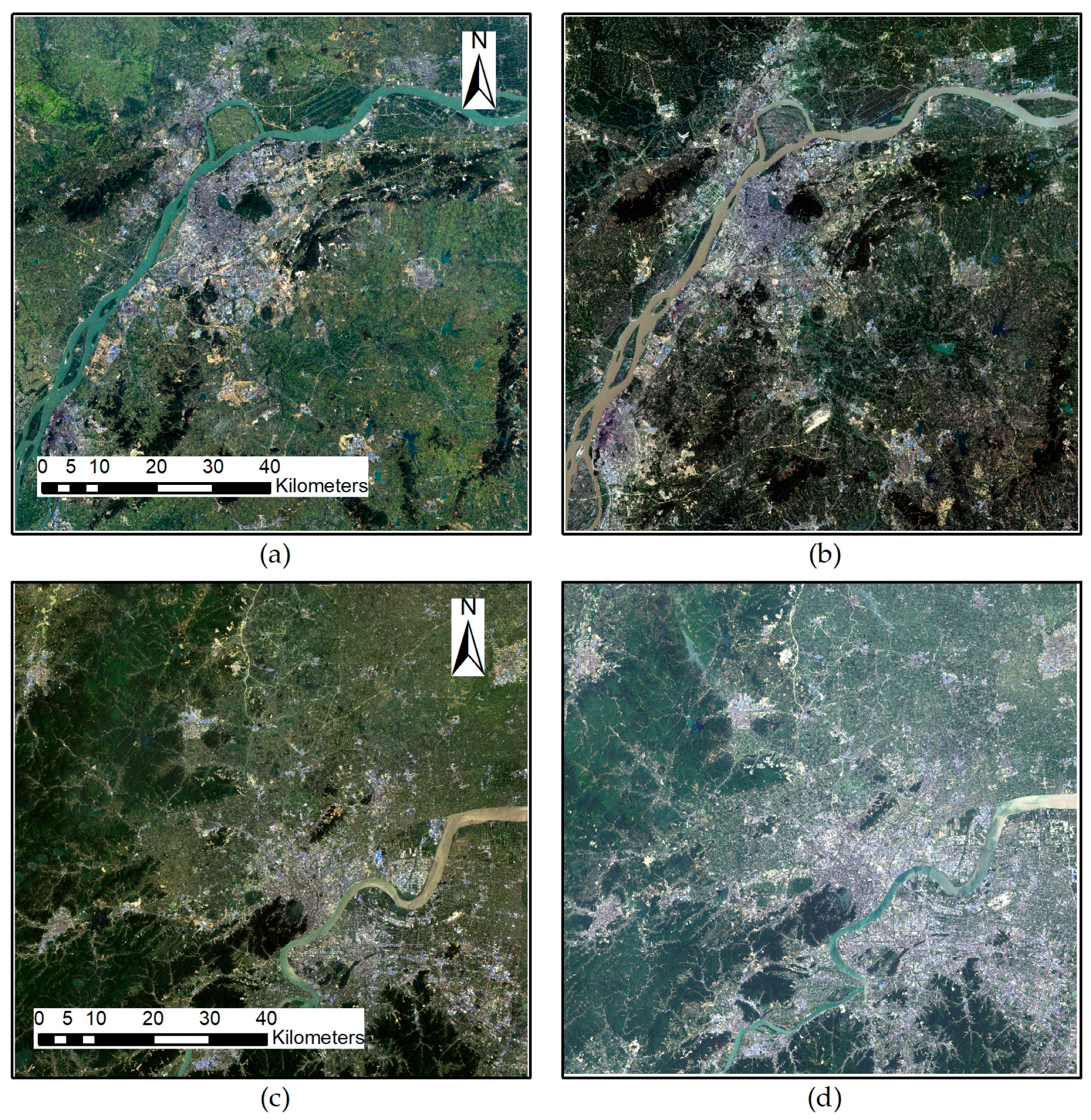
The Landsat satellite data have been archived by the US Geological Survey since 1972. These data are applicable for historical study of land-cover change. The remote sensing images chosen for this study were Landsat 5 and Landsat 8 surface reflectance distributed by USGS EarthExplorer. We created a cloud-free Landsat image dataset for each experimental area of circa 2010 and the year to update. Table 1 lists the acquisition dates of Landsat images used for the study areas, and Figure 2 shows these images.
The GlobeLand30 datasets are open access maps of Earth land-cover and comprise ten types of land-cover, including cultivated land, forest, grassland, water bodies, wetland, artificial surfaces and so on. These datasets were produced by a pixel-object-knowledge-based (POK-based) classification approach for the years 2000 and 2010 [10,22]. More than 20,000 Landsat and Chinese HJ-1 satellite images were used to produce land-cover maps at 30-metre resolution. The overall accuracy of GlobeLand30 in 2010 reaches 80.33% with over 150,000 test samples. GlobeLand30 in 2010 was applied as an original land-cover map, which is valuable for getting the land-cover information.
To facilitate the land-cover classification process, a group of ancillary geospatial products including both digital surface model (DSM) and digital terrain model (DEM) were collected and preprocessed for this research. The DSM was collected from the precise global digital 3D map “ALOS World 3D” developed by the Japan Aerospace Exploration Agency. The DEM was collected from the ASTER Global Digital Elevation Model developed jointly by the Ministry of Economy, Trade, and Industry (METI) of Japan and NASA. Both of the datasets have a horizontal resolution of approximate 30-metres (1 arcsecond in latitude and longitude).

3. Methods

A land-cover updating approach (Figure 3) to find effective samples from an existing land-cover product and transfer them to new images acquired on the same geographical area at different time instants was developed. Let us consider images over two periods, t1 and t2. X1 and X2 are co-registered remote sensing images acquired at time t1 and t2, respectively. There are corresponding existing land-cover products at time t1, labeled P1. The goal of the proposed approach is to produce a land-cover map corresponding to image X2 with the previously available knowledge from X1 and P1. The specific process was as follows:
  • Minimize differences of land-cover information between X1 and P1 by multi-modality remote sensing dataset, and establish strategy to produce a subset of P1. Accordingly, the subset C1 is considered as a more reliable land-cover map of X1.
  • Establish effective method to select better samples rather than randomly selecting from C1 and obtain a reliable training set T1.
  • The pixel labels of X1 which has a high probability to be reliable also for X2 is transferred. Then a training set T2 is obtained.
  • According to the result of step 3, use spatio-spectral image classification method to output the land-cover classification result of X2.

3.1. Land-Cover Optimization Based on Decision Rules

Based on the statistical results of GlobeLand30, it is found that the experimental areas mainly contain six land-cover types, namely cultivated land, forest, grassland, water bodies, wetland and artificial surfaces. Both shrubland and barren land are less than 0.03%. Permanent snow-and-ice and Tundra do not exist in the experimental areas. The aforementioned six land-cover types are enough to constitute the class system of rapidly urbanizing areas and can satisfy the research and application of most urban areas. Therefore, the proposed land-cover optimization strategy only considers decision rules related to these six types.
Note that images used to produce GlobeLand30 are not necessarily the same as those selected for this study. In addition, less than 85% in overall accuracy indicates that there are a number of misclassified patches in land-cover products. In order to minimize the impact of these two factors, a land-cover optimization strategy was proposed by establishing decision rules based on the land-cover information provided by multi-modality datasets.
The development of decision rules integrated the quality-enhanced NTL data, the elevation and slope extracted from DSM and a series of indices extracted from Landsat imagery. Indices related to vegetation, water, and impervious surface were calculated for decision rules. The use of the Normalized Difference Vegetation Index (NDVI) is currently accepted to enhance the difference between vegetation and non-vegetation. The Modified Normalized Difference Water Index (MNDWI) can significantly enhance the water information, especially in urban scenes [46]. The Biophysical Composition Index (BCI) has proved to have a closer relationship with impervious surface abundance than other indices [3]. These three indices were used to aid in the formulation of decision rules.
Based on the prior knowledge, the optimization strategy for six land-cover types was established. The cultivated land class should contain irrigated farmlands, green houses cultivated land, economic cultivated land and others. BCI and NTL can detect some misclassified pixels in cultivated land class, especially rural cottages. Cultivated land is generally cultivated on relatively flat terrain which is different from other vegetation due to human management. Artificial surfaces mainly consist of urban areas, roads, rural cottages and others. Different from other land-cover types, its corresponding pixels usually have large BCI and NTL values and small MNDWI and NDVI values. NDVI can correct classification results of forest and grassland and MNDWI can correct classification results of water bodies. For better optimization results, the other two indices were chosen as decision rules for these three land-cover types. Figure 4 shows the strategy used to optimize the land-cover map.
The variable σi represents the threshold of different characteristics of different land-cover classes. To automatically achieve the land-cover class, the Otsu’s binarization algorithm was applied for threshold decision [47]. The threshold calculation of Otsu’s binarization algorithm can be simply described as follows [47,48]:
T = arg   max [ ω 0 ω 1 ( μ 1 μ 0 ) 2 ]
where T is the required threshold. ω0 and ω1 are the percentages of background pixels and object pixels in the image. μ0 and μ1 are the mean values of the background pixels and object pixels in this image.
An appropriate threshold can be selected by Otsu’s method for two-class segmentation base on an index image, just like vegetation/non-vegetation and water/non-water. In Figure 4, σa-d were calculated by Otsu’s method. However, this method cannot deal with the decision rules with multiple thresholds. Considering that the accuracy of GlobeLand30 product is higher than 80%, it is feasible to generate random labels to determine the remaining thresholds. The maximum or minimum values of sample statistics were selected as the threshold values under the premise of removing the outliers. Based on this study, the maximum or minimum values within the cumulative probability of 5%–95% are recommended.

3.2. Knowledge Transfer Procedure

The aforementioned strategy based on decision rules was used to remove possible misclassified pixels in Globeland30. Furthermore, the workflow of knowledge transfer procedure was designed in this subsection. The workflow (Figure 5) included three main steps: (1) perform Spectral Characteristic-based (SC) clustering using the optimized procedure output; (2) assign a training set T1 using discriminate criterion based on clustering result; (3) identify changed and unchanged regions, and label unchanged pixels from X2 using transferred land-cover knowledge. After the above three steps, the land-cover knowledge from the historical map is transferred to the new satellite image. These three steps are further described below.

3.2.1. Spectral Characteristic-Based Clustering

A wide range of spectral indices taken advantage of the characteristics of the spectral curve shape in different land-cover types has been developed and successfully applied for different land-cover class discrimination purposes. From this perspective, a feature transformation method was defined to depict the spectral curve shape for each pixel [29].
Let X = (x1, x2, …, xM) be the multispectral remote sensing image made up of M pixels and N spectral channels, and xm = {xm,1, xm,2, …, xm,N} denote the mth pixel with N spectral channels. Let S = (s1, s2, …, sM) denote spectral curve shape vectors of the M pixels, and sm = {sm,1, sm,2, …, sm,N(N−1)/2}. sm is a spectral curve vector of the mth pixel. sm is calculated by the equations as follows, where is a binary function:
s m = { f ( x m , q x m , p ) | p < q ; p , q = 1 , 2 , , n }
f ( x ) = { 0 , x < 0 1 , x 0
SC clustering method is shown below. Firstly, for each land-cover class of the optimized procedure output, all initial samples are transformed into a new feature space by equations (2) and (3). Next, samples with exactly the same spectral curve vector are clustered into one subclass. All samples of each clustered subclass are enumerated and sorted by number of pixels to generate the statistical histogram. Finally, the clustered subclasses with a very small number of pixels are removed while the main spectral curve vector subclasses in each land-cover class are retained in the corresponding histogram.

3.2.2. Discriminate Criterion

For the purpose of classification, training samples of different land-cover classes are supposed to have sufficient separability. From this perspective, the discriminate criterion based on class similarity was defined for the output of SC clustering. Therefore, clustering results were further selected based on the discriminate criterion for subclasses in different land-cover classes. Class similarity was measured according to J-M distance [49]. For subclass i and subclass j of different land-cover classes, the J-M distance between them can be calculated as:
J M i j = 2 ( 1 e b i j )
where bij is the Bhattacharyya distance between the aforementioned two classes. Under the assumption of Gaussian distributed classes, Bhattacharyya distance can be calculated as [50]:
b i j = 1 8 ( μ i μ j ) T ( i + j 2 ) 1 ( μ i μ j ) + 1 2 ln ( 1 2 | i + j | | i | | j | )
where μi and μj are the mean vectors of the classes i and j, respectively. ∑i and ∑j are their covariance matrices. The discriminant criterion is as follows. The class similarity of all subclasses except the first class of each histogram is calculated in pairs by J-M distance. For given subclass i and subclass j in different land-cover classes, if the result of J-M distance is lower than a user-defined threshold value which supposed to be 1, this pair is recommended to be removed. The final remaining subclasses make up the training set T1 for X1. In addition, the Section 3.2.1 and Section 3.2.2 can constitute an advanced sample selection method.

3.2.3. Change Detection Technique

Different from other TL methods, training sample labels were transferred by change detection (CD). The land-cover knowledge in an unchanged region is reliable for both X1 and X2. Such information can be represented by the labels of unchanged pixels. Change detection technique is robust to the class statistical distribution differences between the source and target images, and has been widely used in relevant literatures [38,51,52,53]. Change vector analysis (CVA) was chosen for CD because it can take full advantage of the information in all bands of multispectral (MS) images and produce reliable change information. The fundamental theory of CVA can be described as follows [54,55,56]: Let X1 and X2 be two MS images made up of N bands acquired over the same geographical area at time t1 and t2, respectively. The difference image can be calculated by subtracting the two images pixel by pixel:
X D = X 2 X 1
And the change magnitude of mth pixel is defined by the Euclidean distance:
ρ m = n = 1 N ( X D m n ) 2
where ρm is the magnitude and X D m n is the ith pixel in nth (n = 1, 2, …, N) band of XD. A reliable threshold calculated by automatic approach along ρ variable divides the difference image into two parts, the unchanged pixels and changed pixels. This threshold is expected to detect the change pixels between X1 and X2 sufficiently. After testing several automatic threshold algorithms, the Otsu’s method was selected to find the thresholds as well.
From the Section 3.2.1, Section 3.2.2 and Section 3.2.3, the land-cover related knowledge was transferred from historical land-cover map, the training set T2 was collected by the transferred labels. It is worth mentioning that the proposed approach adopts spectral characteristic-based clustering method instead of conventional methods, such as K-means clustering. This makes the process of clustering unnecessary to input any parameters. In addition, the widely used empirical value and automatic threshold selection method completely automate the proposed knowledge transfer procedure.

3.3. Multi-Feature Extraction and Classification

In order to improve the classification performance, spectral features, spectral index images and textural features were computed to form the feature space. Spectral indices were extracted to complement the spectral features. The Normalized Difference Spectral Vector (NDSV) proposed in literature [12,57] was applied in this paper. NDSV would minimize the risk of ambiguities by grouping all possible normalized different indices. NDSV is expressed as follows:
NDSV = [ f ( b 1 , b 2 ) f ( b 1 , b 3 ) f ( b 1 , b j ) f ( b 2 , b 3 ) f ( b i , b j ) ]
f ( b i , b j ) = ( b i b j ) / ( b i + b j )
where bi, bj (i < j) are reflectance values in the ith and jth band of MS image.
The textural features play an important role in distinguish the classes with similar spectral characteristics in MS image classification. The Gray Level Co-occurrence Matrix (GLCM) is the distribution of co-occurring gray values in an image. It calculates the frequency for different combinations of gray values occur in an image [58]. A total of 8 kinds of textural statistics including contrast, dissimilarity, homogeneity, angular second moment, entropy, GLCM mean, variance and correlation derived from GLCM were selected to describe the textural features. The GLCM texture, which is the combination of the above textural statistics, was used to characterize the texture information for all band of OLI image with a window size 3. Considering clear and abundant spatial features of panchromatic band, GLCMs were also extracted from corresponding panchromatic band with a window size 3. All of the above texture statistics together made up the spatial feature space.
In the classifier training procedure, three classification methods were employed to complete classification task. Random Forest (RF) is an ensemble classifier that produces multiple decision trees using a randomly selected subset of training samples and variables [59]. Support Vector Machine (SVM) is a supervised classifier based on empirical risk minimization in which kernel functions are used to the training data to a feature space of a higher dimension [60]. SVM with linear kernel was selected in this study. Besides, another ensemble classifier using bagging method was also considered in due to a large number of samples with relative lower data dimension.

4. Experiments and Results

In the experiments, two Landsat datasets were used to evaluate the performance of the proposed methods. The dataset of Nanjing is composed of Landsat-5 satellite image acquired in 2009 and Landsat-8 satellite image acquired in 2013. The dataset of Hangzhou is covered by Landsat-5 satellite image acquired in 2008 and Landsat-8 satellite image acquired in 2013. In the following, the land-cover optimization results were first presented by comparing the original land-cover products. Then, the reliability of source domain samples selected by our proposed method was assessed using accuracy measures. Finally, the classification results in target image were generated and evaluated by reference data.

4.1. Results of Land-cover Optimization

The initial land-cover product was optimized by the strategy in Section 3.1. The optimized land-cover classes were compared with the original products on the basis of reference images in Table 2. The false-color images of forest and water bodies combines NIR, red and green bands while the others are shown in SWIR, NIR and blue spectral bands. Obviously, the results of cultivated land, water bodies and artificial surfaces are much finer than the initial land-cover product. For cultivated land, the Globeland30 misclassified many small rural cottages and narrow roads as cultivated land. Under the decision rule composed of BCI and NTL, the optimized cultivated land is closer to X1. Due to the time difference between the Globeland30 and X1, the water body changed into cultivated land (paddy fields) and other land-cover types. The proposed decision rule solved this problem by removing the changed region. Compared with the former, the optimized artificial surface removed the confused rivers and urban green land in the city. The optimized forest, grassland and wetland also reduced a considerable number of misclassified pixels by decision rules. The optimization result of wetland is less than satisfactory. Considering it includes multiple forms such as bogs, fens, meadows, marshes, peat land and others, the spectral and spatial diversity within wetland make it difficult to develop effective decision rules. In summary, the proposed land-cover optimization strategy made a contribution in reducing the difference between the product and X1. The optimized land-cover maps can be used to select initial samples.

4.2. Validation of Sample Selection Method

As a key component of the proposed approach, the effect of the sample selection procedure was investigated. A supervised classification result based on Support Vector Machine (SVM) classifier with the modified samples was conducted. The classification result with the initial samples was listed for comparable analysis. As a result, two classification results in both Nanjing and Hangzhou were achieved, respectively. The experimental results of experiment areas are shown in Table 3. The preliminary result is achieved with the initial samples while the SVM-s result is achieved with modified samples.
According to the results presented in Table 3, the accuracy measures increase with the proposed sample selection procedure. In experiment area A, the preliminary result reached the OA of 92.63%, and the improved result reached 94.36%. The corresponding Kappa coefficient also increased from 0.9013 to 0.9246. In experiment area B, the preliminary result had a low accuracy with the OA of 83.52%. With the sample selection procedure, the accuracy of SVM-s result was remarkedly improved to 89.41%. The corresponding Kappa coefficient also increased by nearly 0.1. Overall, the proposed method is sufficient to guarantee the classification result with more efficient samples.

4.3. Results of Updated Land-Cover Map

As the change detection process has been performed, the land-cover knowledge related to X1, which is also reliable for X2 was transferred. Such information is represented by the labels of unchanged regional pixels. So, the training set T2 of X2 was ready for classifying X2. With the feature extraction procedure mentioned in Section 3.3, the feature space with both spatial and spectral features were produced. Considering clear and abundant spatial features of panchromatic band, GLCMs were also extracted from panchromatic bands and the results were resampled into the feature map. The textural statistics results are shown in Table A1, Table A2, Table A3 and Table A4. Table 4 lists all the extracted features for the classification.
About 40,000 samples from the training data set T2 were randomly selected for each experiment area, respectively. Figure 6 shows the result of updated land-cover of two experiment areas, where (a)–(c) are the results of SVM, bagging and RF in Nanjing, and (d)–(f) are the SVM, bagging and RF results in Hangzhou, respectively. For the procedure of accuracy assessment, reference data was collected through visual interpretation of X2 and high-resolution satellite images from google earth close to t2. Finally, more than 30,000 reference samples were collected as test samples to evaluate the performance of classification results. The test samples are shown in the Figure A1.
Table 5 presents the accuracy assessment results. These results indicated that the proposed approach offers a good performance in terms of two accuracy metrics. The OA of all classification results is above 95%, which proves the effectiveness of the proposed method. The classification results based on SVM achieved the best results with the OA of 96.60% and 97.85%. Compared with the other two classifiers, SVM has gained obvious advantages in our study. The classification results obtained based on bagging and RF are close to each other in terms of accuracy, in which the difference of OA is less than 0.4% and the difference of Kappa is less than 0.005. It is worth noting that the results in Hangzhou are significantly better than those in Nanjing. This is most likely due to the difference in the number of test samples between the two regions. There were 21,398 test samples collected in Nanjing, while only 14,034 were collected in Hangzhou. This is because high-resolution images did not completely cover area B, and reliable test samples cannot be obtained in some areas.
In order to analyze the mapping accuracy of individual classes, the confusion matrix based on SVM classification results was calculated. Table 6 and Table 7 show the confusion matrix results. According to the results, the main land-cover classes in the study area, including cultivated land, forest, grassland, and artificial surfaces, have achieved very high class-specific accuracies. Conversely, the accuracies of wetlands and grasslands are relatively lower. Taking Nanjing as an example, the user accuracies (UAs) of these two classes are 77.41% and 80.14%, respectively, which are obviously lower than the other classes. The producer accuracies (PAs) results of these two classes are even lower, with grassland only 69.21% and wetland only 54.53%. These results may be caused by the following two reasons: (1) the proportion of wetland and grassland in the two study areas is very small; (2) the accuracy of grassland and wetland in globeland30 is relatively low indeed.

4.4. Statistics and Analysis

To further evaluate the proposed approach, we applied the feature extraction and classification procedure to the previous Landsat image dataset in study areas. Based on this, land-cover changes in rapidly urbanizing regions can be further analyzed, which shows the potential of the updated land-cover map in application. Figure 7 shows the percentage statistics of each land-cover class of Nanjing and Hangzhou in two periods.
The statistical result in Hangzhou shows the area of artificial surfaces has expanded dramatically from 2008 to 2013 with the cost of decreasing cultivated land, forest, and grassland area. The area of wetland and water bodies also changed slightly due to seasonal changes in water levels, and their total area remained essentially unchanged from 2008 to 2013.
On the contrary, the statistical results in Nanjing are not consistent with the characteristics of rapidly urbanizing regions. Indeed, the artificial surface area has slightly increased and the area of cultivated land has slightly decreased, but it is far less significant than in Hangzhou. In addition, the area of forest and water bodies changed significantly. This is because, in addition to urban expansion; at least two other important factors contribute to land cover change in Nanjing. Urban expansion turned other land-cover types into artificial surfaces. Part of aquaculture land (Aquaculture, also known as aquafarming, is the farming of fish, crustaceans, molluscs, aquatic plants, algae, and other organisms in water bodies), classified as water bodies in Globeland 30 and our classification results, was turned into cultivated land. And part of mining areas, classified as artificial surfaces, was turned into forest in Nanjing from 2008 to 2013. These two factors may be related to local government policies (e.g., arable land minimum and ecological redline policies in China [61]). Different from Hangzhou, the two images in Nanjing were acquired from different seasons, which may also have influenced the classification results. Figure 8 shows the aforementioned three land-cover changes in Nanjing.
From the perspective of urban sprawl, the area of other land-cover types turned into artificial surfaces is calculated. In Nanjing, 428.57 km2 of cultivated land and 37.39 km2 of forest were turned into artificial surfaces, accounting for 87% of new artificial surfaces between 2009 and 2013. In Hangzhou, 454.15 km2 of cultivated land and 34.01 km2 of forest were turned into artificial surfaces, accounting for 89% of new artificial surfaces between 2008 and 2013. Thus, it can be seen that the urban expansion caused considerable area loss of forest and cultivated land in study areas.
Figure 9 shows examples of land-cover change between t1 and t2. Comparing the Landsat images of the two periods, it is found that the cultivated land and forest have shrunk and some small patches disappeared due to dramatic urban sprawl. The growth of artificial surfaces in updated land-cover map accurately matches the spatial pattern of the comparison result between bi-temporal images. The general trend of land-cover change mapped in this study matches visual interpretation of changes from images. In addition, the feature map containing abundant spatial features enables the updated land-cover map to maintain the complete structure and details of main land-cover classes from the vision perspective. Examples in Figure 9 further illustrate the applicability of the proposed approach in rapidly urbanizing regions.

5. Conclusions

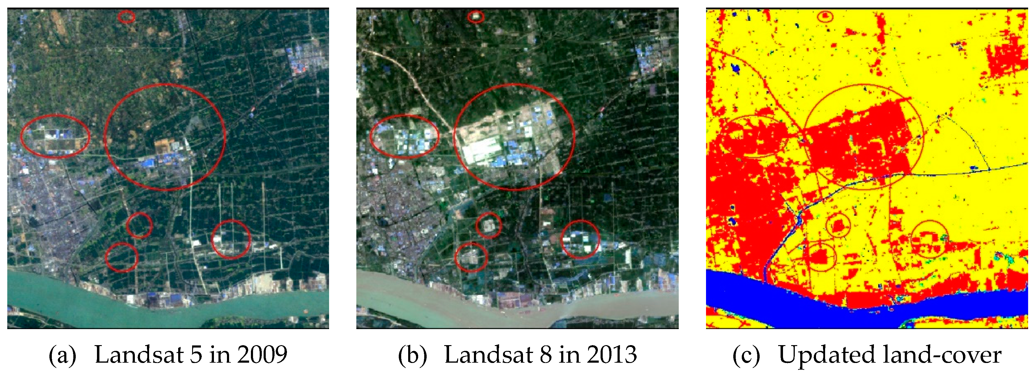
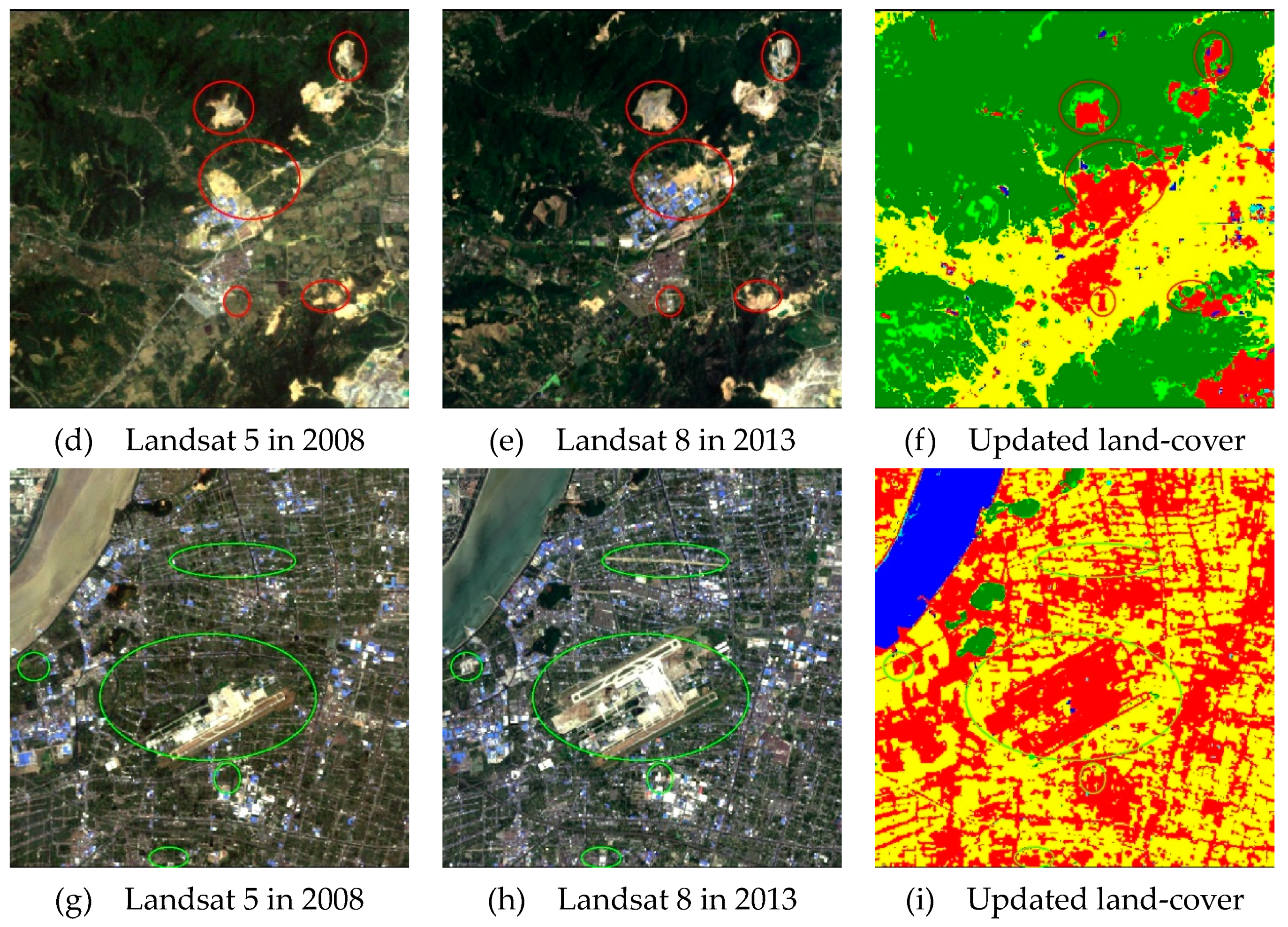
For rapidly urbanizing regions, land-cover mapping is of great importance to urban planning and management. However, land-cover products often have a long renewal cycle and cannot provide timely changes in land-cover information. This study presented a novel automatic approach for updating land-cover map by relational knowledge transfer. It classifies a new satellite image by using the knowledge transferred from existing land-cover product and corresponding image. The proposed approach was defined on the basis of three steps. The first step is devoted to obtain reliable land-cover information from Globeland30. This is done by establishing a set of decision rules based on multi-modality RS datasets to optimize land-cover product. The second step aims at applying proposed knowledge transfer procedure to source domain and target domain, and then transferring land-cover knowledge from modified historical map to new images. With the completion of the multi-feature combination classification procedure, in the third step, the target image is classified to produce the land-cover map. Typical experimental areas, Nanjing and Hangzhou, were selected to proof the effectiveness of the approach. The classification results indicated that the aforementioned steps offer a good performance.
Compared with traditional methods for land-cover mapping, the proposed approach does not involve manual selection of samples and adjustment of variable parameters. Therefore, the method in this study can quickly and effectively produce new land-cover map, which has significant application potential for rapidly urbanizing regions. The characteristics of our study are described below: (1) compared with the existing research on land-cover product update, the uncertainty of existing land-cover map has been fully considered, and the optimized map has been produced instead of directly updating the original map; (2) the knowledge transfer approach in this paper is an unsupervised transfer learning procedure. The training sets for new images are transferred from historical land-cover map automatically; (3) the proposed approach provides a solution for a data-shift problem with its general properties and its simplicity, which has the potential for large-scale operational applications.
In future, more types of geographic information datasets, not limited to remote sensing datasets, could be taken into account in our method for land-cover information transferring. The potential datasets include regional thematic map, open street map and socio-economic data. By combining more land-cover knowledge, the updated maps will hopefully contain more abundant and precise land-cover information.

Author Contributions

Conceptualization, C.L., P.D. and E.L.; methodology, C.L.; validation, C.L., A.S., J.X. and P.D.; data curation, C.L.; writing—original draft preparation, C.L., X.W. and E.L.; writing—review and editing, C.L., P.D. and A.S.; visualization, C.L.; funding acquisition, P.D.

Funding

This study was funded by the National Natural Science Foundation of China (No. 41631176).

Acknowledgments

The authors would like to thank the National Geomatics Center of China (NGCC), U.S. Geological Survey (USGS), National Geophysical Data Center (NGDC), Japan Aerospace Exploration Agency (JAXA), the Ministry of Economy, Trade, and Industry (METI) of Japan and the United States National Aeronautics and Space Administration (NASA) for supporting the used data in this study.

Conflicts of Interest

The authors declare no conflict of interest.

Appendix A. Ground Truth for Study Areas

Figure A1. Ground truth for Nanjing (a) and Hangzhou (b).
Remotesensing 11 01397 g0a1

Appendix B. Results of the Textural Statistics

Table A1. The textural statistics for OLI band 1-4 in Nanjing.
B1B2B3B4
TEX1 Remotesensing 11 01397 i001
TEX2 Remotesensing 11 01397 i002
TEX3 Remotesensing 11 01397 i003
TEX4 Remotesensing 11 01397 i004
TEX5 Remotesensing 11 01397 i005
TEX6 Remotesensing 11 01397 i006
TEX7 Remotesensing 11 01397 i007
TEX8 Remotesensing 11 01397 i008
Table A2. The textural statistics for OLI band 5-7 and panchromatic band in Nanjing.
B5B6B7PAN
TEX1 Remotesensing 11 01397 i009
TEX2 Remotesensing 11 01397 i010
TEX3 Remotesensing 11 01397 i011
TEX4 Remotesensing 11 01397 i012
TEX5 Remotesensing 11 01397 i013
TEX6 Remotesensing 11 01397 i014
TEX7 Remotesensing 11 01397 i015
TEX8 Remotesensing 11 01397 i016
Table A3. The textural statistics for OLI band 1-4 in Hangzhou.
B1B2B3B4
TEX1 Remotesensing 11 01397 i017
TEX2 Remotesensing 11 01397 i018
TEX3 Remotesensing 11 01397 i019
TEX4 Remotesensing 11 01397 i020
TEX5 Remotesensing 11 01397 i021
TEX6 Remotesensing 11 01397 i022
TEX7 Remotesensing 11 01397 i023
TEX8 Remotesensing 11 01397 i024
Table A4. The textural statistics for OLI band 5-7 and panchromatic band in Hangzhou.
B5B6B7PAN
TEX1 Remotesensing 11 01397 i025
TEX2 Remotesensing 11 01397 i026
TEX3 Remotesensing 11 01397 i027
TEX4 Remotesensing 11 01397 i028
TEX5 Remotesensing 11 01397 i029
TEX6 Remotesensing 11 01397 i030
TEX7 Remotesensing 11 01397 i031
TEX8 Remotesensing 11 01397 i032
B1: Coastal aerosol, B2: Blue, B3: Green, B4: Red, B5: NIR, B6: SWIR 1, B7: SWIR 2, PAN: Panchromatic, TEX1: mean, TEX2: variance, TEX3: homogeneity, TEX4: contrast, TEX5: dissimilarity, TEX6: entropy, TEX7: angular second moment, TEX8: correlation.

References

  1. Chandrakant, L. The state of the world population 2007: Unleashing the potential of urban growth. Indian Pediatr. 2008, 45, 481–482. [Google Scholar]
  2. Feyisa, G.L.; Meilby, H.; Darrel Jenerette, G.; Pauliet, S. Locally optimized separability enhancement indices for urban land cover mapping: Exploring thermal environmental consequences of rapid urbanization in Addis Ababa, Ethiopia. Remote Sens. Environ. 2016, 175, 14–31. [Google Scholar] [CrossRef]
  3. Deng, C.; Wu, C. BCI: A biophysical composition index for remote sensing of urban environments. Remote Sens. Environ. 2012, 127, 247–259. [Google Scholar] [CrossRef]
  4. Defries, R.S.; Rudel, T.; Uriarte, M.; Hansen, M. Deforestation driven by urban population growth and agricultural trade in the twenty-first century. Nat. Geosci. 2010, 3, 178–181. [Google Scholar] [CrossRef]
  5. Pribadi, D.O.; Pauleit, S. The dynamics of peri-urban agriculture during rapid urbanization of Jabodetabek Metropolitan Area. Land Use Policy 2015, 48, 13–24. [Google Scholar] [CrossRef]
  6. He, K.; Huo, H.; Zhang, Q. URBANAIRPOLLUTION INCHINA: Current Status, Characteristics, and Progress. Annu. Rev. Energy Environ. 2002, 27, 397–431. [Google Scholar] [CrossRef]
  7. Chen, X.-L.; Zhao, H.-M.; Li, P.-X.; Yin, Z.-Y. Remote sensing image-based analysis of the relationship between urban heat island and land use/cover changes. Remote Sens. Environ. 2006, 104, 133–146. [Google Scholar] [CrossRef]
  8. Frick, A.; Tervooren, S. A Framework for the Long-term Monitoring of Urban Green Volume Based on Multi-temporal and Multi-sensoral Remote Sensing Data. J. Geovisualization Spat. Anal. 2019, 3. [Google Scholar] [CrossRef]
  9. Schneider, A.; Friedl, M.A.; Potere, D. Mapping global urban areas using MODIS 500-m data: New methods and datasets based on ‘urban ecoregions’. Remote Sens. Environ. 2010, 114, 1733–1746. [Google Scholar] [CrossRef]
  10. Chen, J.; Chen, J.; Liao, A.; Cao, X.; Chen, L.; Chen, X.; He, C.; Han, G.; Peng, S.; Lu, M.; et al. Global land cover mapping at 30m resolution: A POK-based operational approach. ISPRS J. Photogramm. Remote Sens. 2015, 103, 7–27. [Google Scholar] [CrossRef] [Green Version]
  11. Liu, X.; Hu, G.; Chen, Y.; Li, X.; Xu, X.; Li, S.; Pei, F.; Wang, S. High-resolution multi-temporal mapping of global urban land using Landsat images based on the Google Earth Engine Platform. Remote Sens. Environ. 2018, 209, 227–239. [Google Scholar] [CrossRef]
  12. Trianni, G.; Angiuli, E. Urban Mapping in Landsat Images Based on Normalized Difference Spectral Vector. IEEE Geosci. Remote Sens. Lett. 2013, 11, 661–665. [Google Scholar]
  13. Zheng, H.; Du, P.; Chen, J.; Xia, J.; Li, E.; Xu, Z.; Li, X.; Yokoya, N. Performance Evaluation of Downscaling Sentinel-2 Imagery for Land Use and Land Cover Classification by Spectral-Spatial Features. Remote Sens. 2017, 9, 1274. [Google Scholar] [CrossRef]
  14. Ban, Y.; Gong, P.; Giri, C. Global land cover mapping using Earth observation satellite data: Recent progresses and challenges. ISPRS J. Photogramm. Remote Sens. 2015, 103, 1–6. [Google Scholar] [CrossRef] [Green Version]
  15. Yang, Y.; Xiao, P.; Feng, X.; Li, H. Accuracy assessment of seven global land cover datasets over China. ISPRS J. Photogramm. Remote Sens. 2017, 125, 156–173. [Google Scholar] [CrossRef]
  16. Hansen, M.C.; Defries, R.S.; Townshend, J.R.G.; Sohlberg, R. Global land cover classification at 1 km spatial resolution using a classification tree approach. Int. J. Remote Sens. 2000, 21, 1331–1364. [Google Scholar] [CrossRef]
  17. Friedl, M.A.; Sulla-Menashe, D.; Tan, B.; Schneider, A.; Ramankutty, N.; Sibley, A.; Huang, X. MODIS Collection 5 global land cover: Algorithm refinements and characterization of new datasets. Remote Sens. Environ. 2010, 114, 168–182. [Google Scholar] [CrossRef]
  18. Pesaresi, M.; Huadong, G.; Blaes, X.; Ehrlich, D.; Ferri, S.; Gueguen, L.; Halkia, M.; Kauffmann, M.; Kemper, T.; Lu, L.; et al. A Global Human Settlement Layer From Optical HR/VHR RS Data: Concept and First Results. IEEE J. Sel. Top. Appl. Earth Obs. Remote Sens. 2013, 6, 2102–2131. [Google Scholar] [CrossRef]
  19. Esch, T.; Marconcini, M.; Felbier, A.; Roth, A.; Heldens, W.; Huber, M.; Schwinger, M.; Taubenböck, H.; Müller, A.; Dech, S.J.I.G.; et al. Urban Footprint Processor-Fully Automated Processing Chain Generating Settlement Masks From Global Data of the TanDEM-X Mission. IEEE Geosci. Remote Sens. Lett. 2013, 10, 1617–1621. [Google Scholar] [CrossRef]
  20. Esch, T.; Heldens, W.; Hirne, A.; Keil, M.; Marconcini, M.; Roth, A.; Zeidler, J.; Dech, S.; Strano, E.; Sensing, R. Breaking new ground in mapping human settlements from space. Glob. Urban Footpr. 2017, 134, 30–42. [Google Scholar]
  21. Wang, P.; Huang, C.; Tilton, J.C.; Tan, B.; Colstoun, E.C.B.D. HOTEX: An approach for global mapping of human built-up and settlement extent. In Proceedings of the 2017 IEEE International Geoscience and Remote Sensing Symposium, Fort Worth, TX, USA, 23–28 July 2017. [Google Scholar]
  22. Chen, J.; Ban, Y.; Li, S. China: Open access to Earth land-cover map. Nature 2015, 514, 434. [Google Scholar]
  23. Zhang, X.; Li, P. A temperature and vegetation adjusted NTL urban index for urban area mapping and analysis. ISPRS J. Photogramm. Remote Sens. 2018, 135, 93–111. [Google Scholar] [CrossRef]
  24. Crawford, M.M.; Tuia, D.; Yang, H.L. Active Learning: Any Value for Classification of Remotely Sensed Data? Proc. IEEE 2013, 101, 593–608. [Google Scholar] [CrossRef] [Green Version]
  25. Demir, B.; Bovolo, F.; Bruzzone, L. Classification of time series of multispectral images with limited training data. IEEE Trans. Image Process. A Publ. IEEE Signal Process. Soc. 2013, 22, 3219–3233. [Google Scholar] [CrossRef] [PubMed]
  26. Tuia, D.; Volpi, M.; Copa, L.; Kanevski, M.; Munoz-Mari, J. A Survey of Active Learning Algorithms for Supervised Remote Sensing Image Classification. IEEE J. Sel. Top. Signal Process. 2011, 5, 606–617. [Google Scholar] [CrossRef]
  27. Huang, C.; Song, K.; Kim, S.; Townshend, J.R.; Davis, P.; Masek, J.G.; Goward, S.N. Use of a dark object concept and support vector machines to automate forest cover change analysis. Remote Sens. Environ. 2008, 112, 970–985. [Google Scholar] [CrossRef]
  28. Ma, X.; Tong, X.; Liu, S.; Luo, X.; Xie, H.; Li, C. Optimized Sample Selection in SVM Classification by Combining with DMSP-OLS, Landsat NDVI and GlobeLand30 Products for Extracting Urban Built-Up Areas. Remote Sens. 2017, 9, 236. [Google Scholar] [CrossRef]
  29. Li, E.; Du, P.; Samat, A.; Xia, J.; Che, M. An automatic approach for urban land-cover classification from Landsat-8 OLI data. Int. J. Remote Sens. 2015, 36, 5983–6007. [Google Scholar] [CrossRef]
  30. Tuia, D.; Persello, C.; Bruzzone, L. Domain Adaptation for the Classification of Remote Sensing Data: An Overview of Recent Advances. IEEE Geosci. Remote Sens. Mag. 2016, 4, 41–57. [Google Scholar] [CrossRef]
  31. Olthof, I.; Butson, C.; Fraser, R. Signature extension through space for northern landcover classification: A comparison of radiometric correction methods. Remote Sens. Environ. 2005, 95, 290–302. [Google Scholar] [CrossRef]
  32. Rakwatin, P.; Takeuchi, W.; Yasuoka, Y. Stripe Noise Reduction in MODIS Data by Combining Histogram Matching With Facet Filter. IEEE Trans. Geosci. Remote Sens. 2007, 45, 1844–1856. [Google Scholar] [CrossRef]
  33. Deng, J.S.; Wang, K.; Deng, Y.H.; Qi, G.J. PCA-based land-use change detection and analysis using multitemporal and multisensor satellite data. Int. J. Remote Sens. 2008, 29, 4823–4838. [Google Scholar] [CrossRef]
  34. Zanchetta, A.; Bitelli, G.; Karnieli, A. Monitoring desertification by remote sensing using the Tasselled Cap transform for long-term change detection. Nat. Hazards 2016, 83, 223–237. [Google Scholar] [CrossRef]
  35. Pan, S.J.; Yang, Q. A Survey on Transfer Learning. IEEE Trans. Knowl. Data Eng. 2010, 20, 1345–1359. [Google Scholar] [CrossRef]
  36. Bruzzone, L.; Marconcin, M. Toward the Automatic Updating of Land-Cover Maps by a Domain-Adaptation SVM Classifier and a Circular Validation Strategy. IEEE Trans. Geosci. Remote Sens. 2009, 47, 1108–1122. [Google Scholar] [CrossRef]
  37. Persello, C.; Bruzzone, L. Active Learning for Domain Adaptation in the Supervised Classification of Remote Sensing Images. IEEE Trans. Geosci. Remote Sens. 2012, 50, 4468–4483. [Google Scholar] [CrossRef]
  38. Demir, B.; Bovolo, F.; Bruzzone, L. Updating Land-Cover Maps by Classification of Image Time Series: A Novel Change-Detection-Driven Transfer Learning Approach. IEEE Trans. Geosci. Remote Sens. 2013, 51, 300–312. [Google Scholar] [CrossRef]
  39. Samat, A.; Gamba, P.; Abuduwaili, J.; Liu, S.; Miao, Z. Geodesic Flow Kernel Support Vector Machine for Hyperspectral Image Classification by Unsupervised Subspace Feature Transfer. Remote Sens. 2016, 8, 234. [Google Scholar] [CrossRef]
  40. Li, X.; Zhang, L.; Du, B.; Zhang, L.; Shi, Q. Iterative Reweighting Heterogeneous Transfer Learning Framework for Supervised Remote Sensing Image Classification. IEEE J. Sel. Top. Appl. Earth Obs. Remote Sens. 2017, 10, 2022–2035. [Google Scholar] [CrossRef]
  41. Sinno Jialin, P.; Tsang, I.W.; Kwok, J.T.; Qiang, Y. Domain adaptation via transfer component analysis. IEEE Trans. Neural Netw. 2011, 22, 199–210. [Google Scholar]
  42. Tuia, D.; Volpi, M.; Trolliet, M.; Camps-Valls, G. Semisupervised Manifold Alignment of Multimodal Remote Sensing Images. IEEE Trans. Geosci. Remote Sens. 2014, 52, 7708–7720. [Google Scholar] [CrossRef]
  43. Samat, A.; Persello, C.; Gamba, P.; Liu, S.; Abuduwaili, J.; Li, E. Supervised and Semi-Supervised Multi-View Canonical Correlation Analysis Ensemble for Heterogeneous Domain Adaptation in Remote Sensing Image Classification. Remote Sens. 2017, 9, 337. [Google Scholar] [CrossRef]
  44. Zhou, Y.; Li, X.; Asrar, G.R.; Smith, S.J.; Imhoff, M. A global record of annual urban dynamics (1992–2013) from nighttime lights. Remote Sens. Environ. 2018, 219, 206–220. [Google Scholar] [CrossRef]
  45. Zhang, Q.; Pandey, B.; Seto, K.C. A Robust Method to Generate a Consistent Time Series From DMSP/OLS Nighttime Light Data. IEEE Trans. Geosci. Remote Sens. 2016, 54, 5821–5831. [Google Scholar] [CrossRef]
  46. XU, H. A Study on Information Extraction of Water Body with the Modified Normalized Difference Water Index (MNDWI). J. Remote Sens. 2005, 9, 589–595. [Google Scholar]
  47. Otsu, N. A Threshold Selection Method from Gray-Level Histograms. IEEE Trans. Syst. Man Cybern. 1979, 9, 62–66. [Google Scholar] [CrossRef] [Green Version]
  48. Xie, H.; Luo, X.; Xu, X.; Pan, H.; Tong, X. Evaluation of Landsat 8 OLI imagery for unsupervised inland water extraction. Int. J. Remote Sens. 2016, 37, 1826–1844. [Google Scholar] [CrossRef]
  49. Bruzzone, L.; Roli, F.; Serpico, S.B. An Extension of the Jeffreys-Matusita Distance to Multiclass Cases for Feature Selection. IEEE Trans. Geosci. Remote Sens. 1995, 33. [Google Scholar] [CrossRef]
  50. Poth, A.; Klaus, D.; Voß, M.; Stein, G. Optimization at multi-spectral land cover classification with fuzzy clustering and the Kohonen feature map. Int. J. Remote Sens. 2010, 22, 1423–1439. [Google Scholar] [CrossRef]
  51. Chen, X.; Chen, J.; Shi, Y.; Yamaguchi, Y. An automated approach for updating land cover maps based on integrated change detection and classification methods. ISPRS J. Photogramm. Remote Sens. 2012, 71, 86–95. [Google Scholar] [CrossRef]
  52. Hu, Y.; Dong, Y. An automatic approach for land-change detection and land updates based on integrated NDVI timing analysis and the CVAPS method with GEE support. ISPRS J. Photogramm. Remote Sens. 2018, 146, 347–359. [Google Scholar] [CrossRef]
  53. Jin, S.; Yang, L.; Zhu, Z.; Homer, C. A land cover change detection and classification protocol for updating Alaska NLCD 2001 to 2011. Remote Sens. Environ. 2017, 195, 44–55. [Google Scholar] [CrossRef]
  54. Du, P.; Liu, S.; Xia, J.; Zhao, Y. Sicong Information fusion techniques for change detection from multi-temporal;remote sensing images. Inf. Fusion 2013, 14, 19–27. [Google Scholar] [CrossRef]
  55. Liu, S.; Bruzzone, L.; Bovolo, F.; Du, P. Hierarchical Unsupervised Change Detection in Multitemporal Hyperspectral Images. IEEE Trans. Geosci. Remote Sens. 2014, 53, 244–260. [Google Scholar]
  56. Lu, D.; Mausel, P.; Brondízio, E.; Moran, E. Change detection techniques. Int. J. Remote Sens. 2010, 25, 2365–2401. [Google Scholar] [CrossRef]
  57. Patel, N.N.; Angiuli, E.; Gamba, P.; Gaughan, A.; Lisini, G.; Stevens, F.R.; Tatem, A.J.; Trianni, G. Multitemporal settlement and population mapping from Landsat using Google Earth Engine. Int. J. Appl. Earth Obs. Geoinf. 2015, 35, 199–208. [Google Scholar] [CrossRef] [Green Version]
  58. Zhong, Y.; Jia, T.; Zhao, J.; Wang, X.; Jin, S. Spatial-Spectral-Emissivity Land-Cover Classification Fusing Visible and Thermal Infrared Hyperspectral Imagery. Remote Sens. 2017, 9, 910. [Google Scholar] [CrossRef]
  59. Belgiu, M.; Drăguţ, L. Random forest in remote sensing: A review of applications and future directions. ISPRS J. Photogramm. Remote Sens. 2016, 114, 24–31. [Google Scholar] [CrossRef]
  60. Xia, J.; Chanussot, J.; Du, P.; He, X. Rotation-Based Support Vector Machine Ensemble in Classification of Hyperspectral Data With Limited Training Samples. IEEE Trans. Geosci. Remote Sens. 2016, 54, 1519–1531. [Google Scholar] [CrossRef]
  61. Bai, Y.; Jiang, B.; Wang, M.; Li, H.; Alatalo, J.M.; Huang, S. New ecological redline policy (ERP) to secure ecosystem services in China. Land Use Policy 2016, 55, 348–351. [Google Scholar] [CrossRef] [Green Version]
Figure 1. Location of the study areas and multi-modality remote sensing datasets in 2010. (A) Nanjing; (B) Hangzhou.
Remotesensing 11 01397 g001
Figure 2. Cloud-free Landsat image datasets for study areas. (a) Nanjing 2009, (b) Nanjing 2013, (c) Hangzhou 2008 and (d) Hangzhou 2013.
Remotesensing 11 01397 g002
Figure 3. Workflow of the proposed approach.
Remotesensing 11 01397 g003
Figure 4. Decision rules applied to optimize Globeland30.
Remotesensing 11 01397 g004
Figure 5. Flowchart showing the three major steps of the knowledge transfer procedure.
Remotesensing 11 01397 g005
Figure 6. Classification results for Target images. (a) Nanjing result by Support Vector Machine (SVM), (b) Nanjing result by bagging, (c) Nanjing result by RF, (d) Hangzhou result by SVM, (e) Hangzhou result by bagging, (f) Hangzhou result by RF.
Remotesensing 11 01397 g006
Figure 7. Percentage statistics for land-cover classification (a) Nanjing 2009, (b) Nanjing 2013, (c) Hangzhou 2008 and (d) Hangzhou 2013.
Remotesensing 11 01397 g007
Figure 8. Three Land-cover change types in Nanjing from bi-temporal images, (a,d) other land-cover types to artificial surfaces, (b,e) aquaculture land to cultivated land, (c,f) mining areas to forest.
Remotesensing 11 01397 g008
Figure 9. Updated land-cover and bi-temporal images for subset areas.
Remotesensing 11 01397 g009aRemotesensing 11 01397 g009b
Table 1. Detailed information on experimental Landsat images.
No.SatelliteObservation DateLocation
1Landsat-5April 2009Nanjing
2Landsat-8August 2013Nanjing
3Landsat-5July 2008Hangzhou
4Landsat-8July 2013Hangzhou
Table 2. Comparison of typical areas before and after optimization.
TypeImagesGlobeland30Optimized
Cultivated land Remotesensing 11 01397 i033
Forest Remotesensing 11 01397 i034
Grassland Remotesensing 11 01397 i035
Wetland Remotesensing 11 01397 i036
Water bodies Remotesensing 11 01397 i037
Artificial surfaces Remotesensing 11 01397 i038
Table 3. Accuracy assessment of results with and without sample selection method.
AssessmentTest Accuracy
NanjingHangzhou
Preliminary ResultSVM-s ResultPreliminary ResultSVM-s Result
OA92.63%94.36%83.52%89.41%
kappa0.90130.92460.75960.8484
Table 4. Overview of extracted features for target image classification.
FeaturesNo.Description
OLI band1-77Landsat 8 surface reflectance
Spectral features21NDSV derived from all possible band combinations
Spatial features64Mean, variance, homogeneity, contrast, dissimilarity, entropy, angular, second moment and correlation derived from GLCM
Topographic features2Elevation and slope information
Total94——
Table 5. Accuracy assessment results for target images.
Experiment AreaSVMBaggingRF
OA (%)KappaOA (%)KappaOA (%)Kappa
A96.600.955095.100.935395.480.9402
B97.850.968097.400.961497.310.9601
Table 6. Confusion matrix of land-cover classification in Nanjing using SVM classifier.
Reference DataTotalUA (%)
CLForestGLWLWBAS
CL6753781411602696396.98
Forest414579109900473896.64
GL08228100036377.41
WL90034307642880.14
WB20015433113347095.42
AS2402705403543699.39
Total682947394066293311548421,398
PA (%)98.8996.6269.2154.5310098.52 96.60
Table 7. Confusion matrix of land-cover classification in Hangzhou using SVM classifier.
Reference DataTotalUA (%)
CLForestGLWLWBAS
CL6129010011614199.80
Forest634500155000471895.38
GL082332000332100
WL220014403019673.47
WB7001480348898.36
AS702502147215999.44
Total62284500488150480218814,034
PA (%)98.4110068.039610098.13 97.85
CL: Cultivated land, GL: grassland, WL: wetland, WB: water bodies, AS: artificial surfaces, PA: Producer accuracy, UA: user accuracy.

