Land Cover Classification from fused DSM and UAV Images Using Convolutional Neural Networks

Abstract

In recent years, remote sensing researchers have investigated the use of different modalities (or combinations of modalities) for classification tasks. Such modalities can be extracted via a diverse range of sensors and images. Currently, there are no (or only a few) studies that have been done to increase the land cover classification accuracy via unmanned aerial vehicle (UAV)–digital surface model (DSM) fused datasets. Therefore, this study looks at improving the accuracy of these datasets by exploiting convolutional neural networks (CNNs). In this work, we focus on the fusion of DSM and UAV images for land use/land cover mapping via classification into seven classes: bare land, buildings, dense vegetation/trees, grassland, paved roads, shadows, and water bodies. Specifically, we investigated the effectiveness of the two datasets with the aim of inspecting whether the fused DSM yields remarkable outcomes for land cover classification. The datasets were: (i) only orthomosaic image data (Red, Green and Blue channel data), and (ii) a fusion of the orthomosaic image and DSM data, where the final classification was performed using a CNN. CNN, as a classification method, is promising due to hierarchical learning structure, regulating and weight sharing with respect to training data, generalization, optimization and parameters reduction, automatic feature extraction and robust discrimination ability with high performance. The experimental results show that a CNN trained on the fused dataset obtains better results with Kappa index of ~0.98, an average accuracy of 0.97 and final overall accuracy of 0.98. Comparing accuracies between the CNN with DSM result and the CNN without DSM result for the overall accuracy, average accuracy and Kappa index revealed an improvement of 1.2%, 1.8% and 1.5%, respectively. Accordingly, adding the heights of features such as buildings and trees improved the differentiation between vegetation specifically where plants were dense.

1. Introduction

In the past few years, unmanned aerial vehicles (UAVs) have been extensively used to collect image data over inaccessible/remote areas [1,2,3]. Ease-of-use and affordability are two catalysing factors for the widespread use of UAVs in civilian and military applications [1,4]. Images captured using UAVs are used for geographical information system databases, datasets for automated decision-making, agricultural mapping, urban planning, land use and land cover detection and environmental monitoring and assessment [1,5,6,7]. Such images are commonly used in supervised machine learning-based classification tasks as training data [8,9,10]. One reason for this is that these images have high resolution and a good range of spectral bands [6]. This is an advantage since training and validating a supervised classifier for a remote sensing task demands reliable features. Due to the quality of UAV images nowadays, extracting reliable features to form a dataset becomes less of a problem. Example of such features are land cover characteristics (geometrical and spectral) from Light Detection and Ranging (LiDAR) and hyperspectral data [11]. Moreover, to enhance land cover classification, the combination of multisource (active/passive sensors) or multimodal data (data with different characteristics) is recommended [12,13]. For example, Jahan et al. [11] fused different LiDAR and hyperspectral datasets, and their derivatives, and proved that the overall accuracy of the fused datasets are higher than the single dataset. Another fusion of LiDAR and aerial colour images was performed to enhance building and vegetation detection [11]. These additional features can sometimes improve the classification accuracy for specific domains and use cases. For example, dataset fusion of RGB (Red, Green and Blue) images obtained from UAVs or other sources together with elevation information from digital surface models (DSM) provided a more holistic representation for the construction of accurate maps [11]. Considering DSMs as additional features was shown to improve classification results for image segmentation [14].

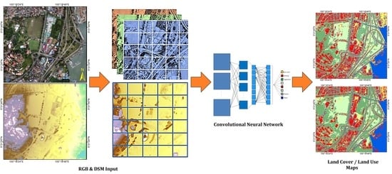
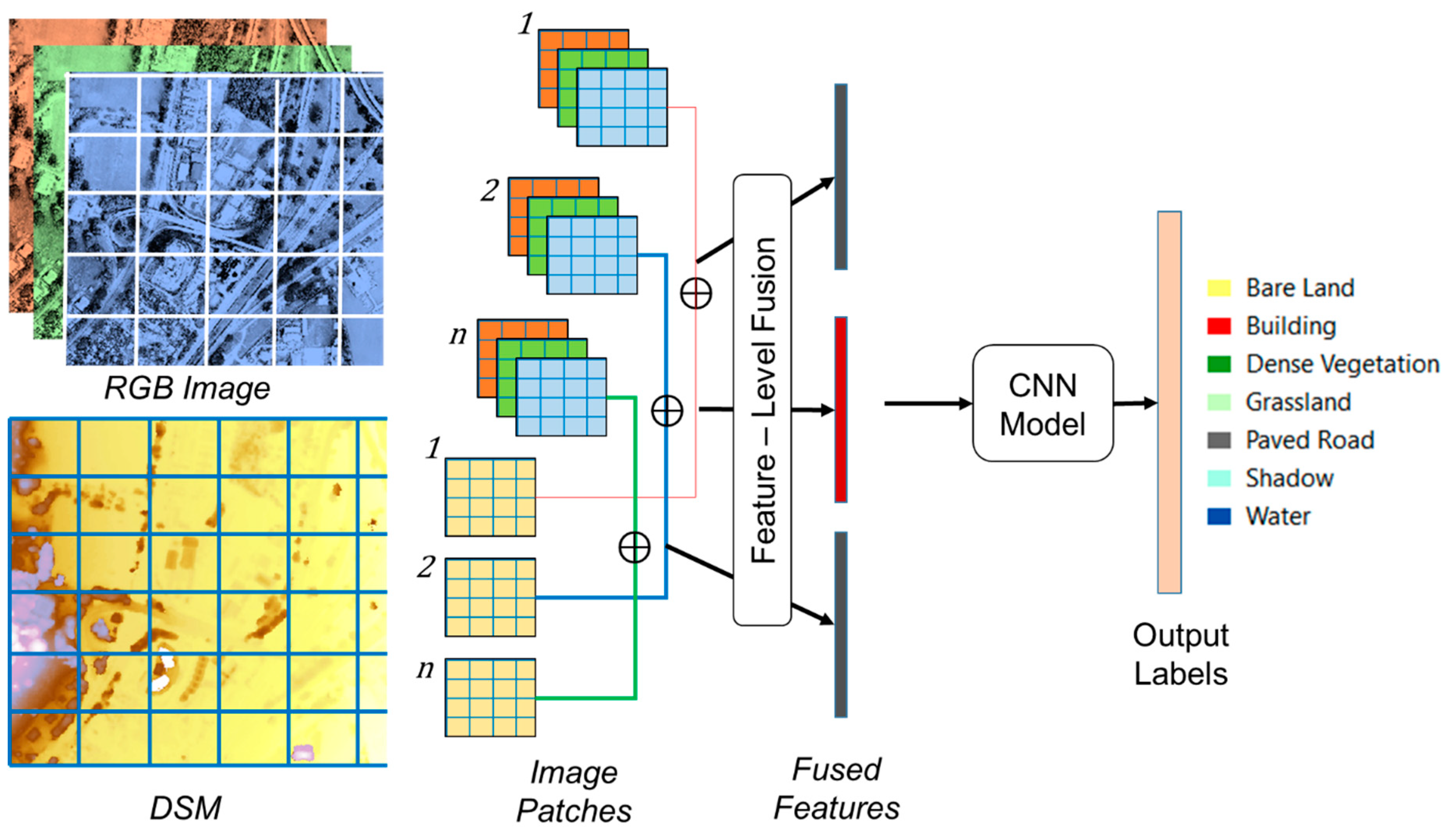
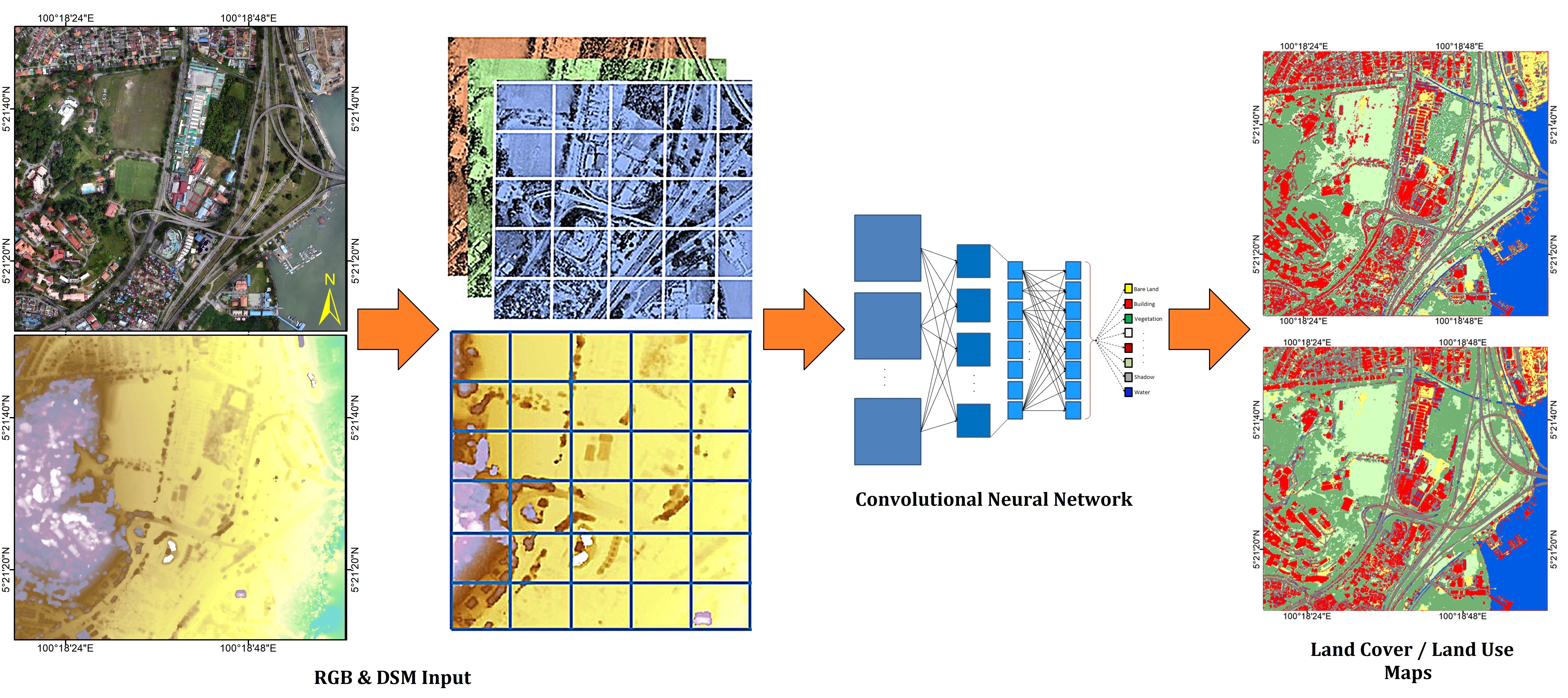
Based on the success of previous studies [11,15,16,17], this paper also examines feature fusion but for the specific task of land cover classification taking advantage of fused DSM–UAV images. Specifically, we investigated the effectiveness of using a single feature modality (RGB data only) versus the fusion of RGB and DSM data. The classification algorithm used to compare the two datasets is a convolutional neural network (CNN), which is a deep-learning technique that hierarchically learns representations from training data, regulates and shares the weight with respect to the training data, generalizes, optimizes, and reduces the parameters with the higher ability to discriminate and extract features, automatically [18,19]. The specific land cover classifications that we considered were: (i) bare land, (ii) buildings, (iii) dense vegetation/trees, (iv) grassland, (v) paved roads, (vi) shadows, and (vii) water bodies.

2. Related Studies

Several studies have been conducted using different approaches and models for tasks such as land use land cover and crops classification. These studies have primarily varied according to the technique used. Reference [20] developed a hybrid model based on the integration of random forest and a texture analysis to classify urban-vegetated areas. Their model contained 200 decision trees trained on hand-crafted spectral–textural features. The highest accuracy reported was 90.6%. The work in [21] used a multiple kernel-learning (MKL) model to classify UAV data in Kigali, Rwanda. Their model showed superior classification performance (90.6% accuracy) and outperformed the single standard single-kernel Support Vector Machine model by 5.2%. In another study [22], a classification framework based on deep-learning and an object-based image analysis (OBIA) proposed to classify UAV data into five categories, namely, water, roads, green land, buildings, and bare land. The proposed framework first performed graph-based minimal spanning-tree segmentation, followed by spatial, spectral, and texture feature extraction from each object. The features were fed into a stacked autoencoder (SAE) for training and achieved an overall accuracy of 97%.

Recently, cameras mounted on UAVs have enabled the acquisition of higher quality images from remote locations, especially those of wet and cropland images. Machine learning has also played an important role, where algorithms such as Support Vector Machine (SVM), Logistic Regression and Artificial Neural Networks (ANN) have been used to perform automatic land classification [23,24]. Lie et al. [25] used high-quality images with OBIA based on multi-view information. They classified wetlands in Florida, USA, into seven classes, namely, Cogon grass, improved pasture, Saw Palmetto shrubland, broadleaf emergent marsh, graminoid freshwater marsh, hardwood hammock–pine, forest, and shadows with an overall accuracy of 80.4%, a user accuracy of 89.7%, and a producer accuracy of 93.3%. Reference [26] developed a model combining deep CNNs with OBIA to create land cover maps from high resolution UAV images with a very good overall accuracy of 82.08%.

The work in [27] developed a model based on conditional random fields where they integrated multi-view and context information. Their work looked at different classifiers, namely, the Gaussian mixed model (GMM), random forests (RF), SVM and DCNN. Machine learning algorithms seem to provide very good classification accuracy, with GMM and DCNN outperforming the rest. Reference [28] evaluated classifications after applying an advanced feature selection model to SVM and RF classifiers. A novel method was developed in [6] where the fuzzy unordered rule algorithm and OBIA were integrated to extract land cover from UAV images. Their method first segments the images based on multi-resolution segmentation, then optimises them based on feature selection (integrating feature space optimisation into the plateau objective function) and finally classifies them using a decision tree and an SVM. Overall accuracy was reported to be 91.23%. Very-high resolution aerial images were classified using a CNN in [29], which has been shown to be effective for the extraction of specific objects such as cars. In another study [18], the capability of CNN to classify aerial photos (with 10 cm resolution) was examined and verified using medium-scale datasets.

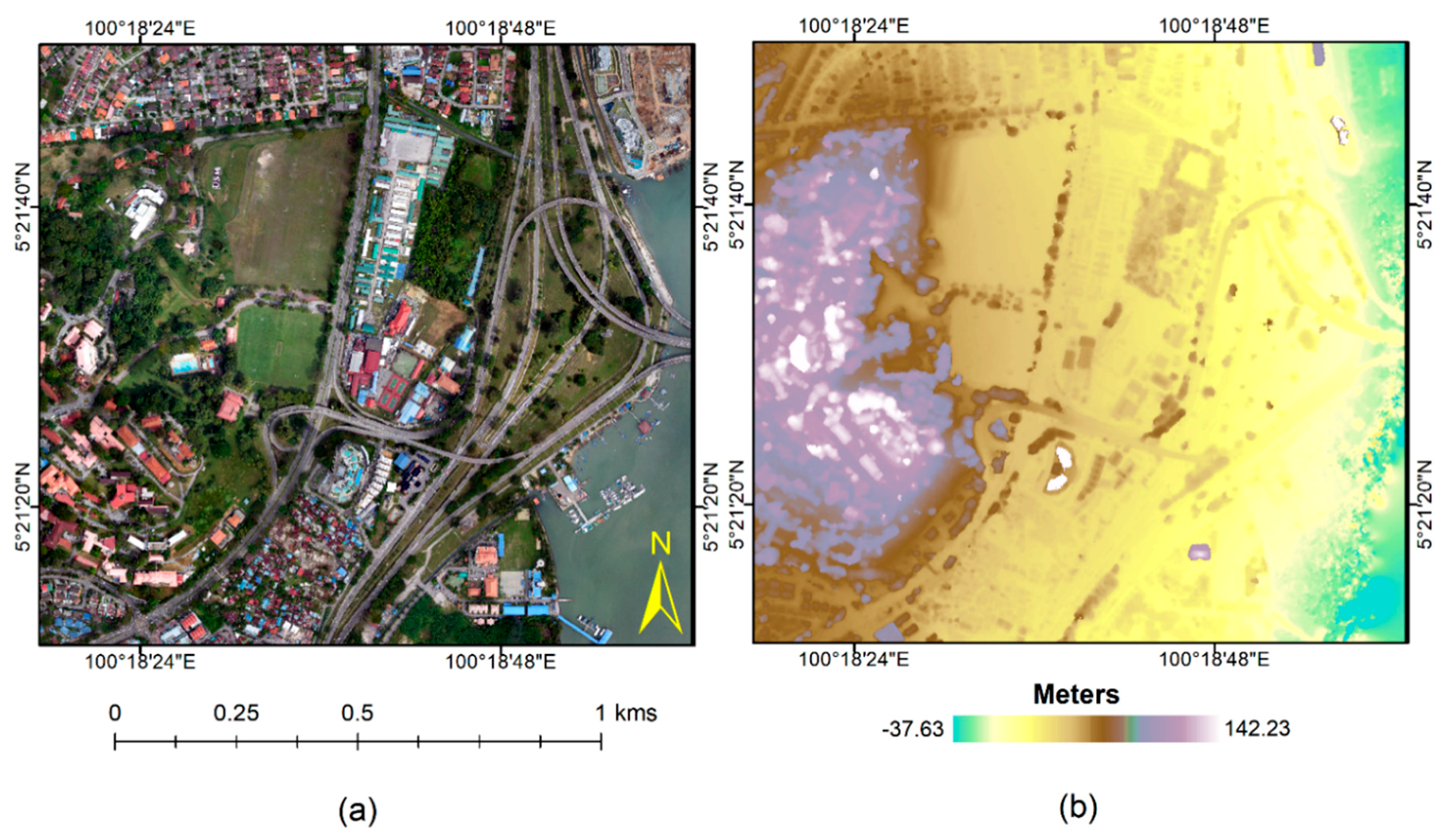
To the best of our knowledge, CNNs have not yet been applied to fused DSM and UAV datasets for land cover classification. Because the resolution of the imagery directly affects the accuracy of the land cover classification, we applied a CNN algorithm to the fusion of a UAV image and DSM (both with 0.8 m/pixel resolution) for urban feature extraction to inspect the accuracy of the result. In general, UAV datasets have lower resolution and accuracy compared to aerial photos [30]. Therefore, this study looks at improving the accuracy by exploiting CNNs for these datasets. The following sections explain and discuss the state of the art with respect to classifying UAV datasets with a focus on deep-learning-based methods.

3. Materials and Methods

3.1. UAV Data Acquisition

The UAV dataset used in this study was acquired over the Universiti Sains Malaysia campus on 3 February 2018 at 12:00 am (Figure 1). The data acquisition was performed using a UAV flying at an altitude of 353 m using a Canon PowerShot SX230 HS (5 mm). The images were characterised by three channels (RGB) with a ground resolution of approximately 9.95 cm/pixel, a 4000 × 3000-pixel resolution and an 8-bit radiometric resolution. An orthomosaic photo was produced from the captured image sequence with Average Root Mean Square Errors (RMSE) of 0.192894 m (1.08795 pix). A DSM was also generated using Agisoft PhotoScan Professional (version 1.3.4, http://www.agisoft.com). The selected subset covers approximately 1.68 km². The point clouds produced by Agisoft had a point density of approximately 1.58 points/m², and the resolution of the DSM was 79.6 cm/pixel.

3.2. Ground Truth Data

A total of 412 ground truth (GT) data (totalling 15,550 pixels) were sampled from Google Earth images. Each sample was labelled according to its respective class. For verification purposes, a filed survey was conducted to verify that the Google Earth samples matched the onsite class labels. The seven land cover classes considered in this work were: (i) bare land, (ii) buildings, (iii) dense vegetation/trees, (iv) grassland, (v) paved roads, (vi) shadows, and (vii) water bodies. The details for the GT data is shown in

Table 1. Number of regions of interest (ROIs) and pixels per land cover class in the ground truth (GT) dataset.

Land Cover Class	Number of ROIs	Number of Pixels
Bare land	27	1104
Buildings	129	3833
Dense vegetation/trees	53	1917
Grassland	47	3094
Paved roads	92	1343
Shadows	36	76
Water bodies	28	4183

.

Training, Validation and Testing Set

From the above dataset, 50% was allocated for training, 25% for validation, and the remaining 25% was used as a random test. Each set is explained in the following paragraphs. The training dataset is used to train the CNN. In general, the training set contained labelled instances that were known to the classifier. At each training iteration, the model performed classification for all instances of the input (one iteration involving all dataset instances is called an epoch) based on the initial weights of the network. A loss value was associated with each epoch, which represents the error between CNN’s predictions and the actual class labels. After the predetermined number of epochs was reached, the weights in the network were updated accordingly via an algorithm such as Stochastic or Batch Gradient Descent. The ultimate goal for training is for the error to be minimized, or a stopping criterion to be reached.

The validation set, whose labels are also known to the classifier, serves two purposes. The first is to ensure the model does not overfit the data in the training set. The second purpose is to aid any necessary hyperparameter tuning. In CNNs, hyperparameters are settings that can be manipulated to ensure the best output. Example hyperparameters are the learning rate, number of epochs, number of hidden layers, activation function choices, and batch size. During the training process, the results from the validation set (such as the validation loss and validation accuracy) can be monitored in order to determine whether any hyperparameters need to be tweaked. The CNN weights however are not updated based on the validation loss.

The test set is a set unseen by the CNN (i.e., labels are not visible). After the CNN produced satisfactory results based on the training and validation sets, it was then evaluated on the test set. Having a good and randomized test set (while still adhering to the distribution and assumptions of the original problem) can be very useful especially if a classifier is to be deployed in real-world situations. In our work, the test set was used to ultimately verify the accuracy of our CNN model.

3.3. Image Pre-Processing

Image pre-processing is done to prepare the image data for CNN. This was mainly done using existing packages and software such as ArGIS, Agisoft PhotoScan Professional and Python coding. The Agisoft PhotoScan allows the creation of georeferenced dense point clouds, textured polygonal models, digital elevation models (DEMs), and orthomosaics from a set of overlapping images with the corresponding referencing information [6]. Orthomosaic images and the DSM of the study area were firstly calibrated interior and exterior camera calibrations followed by image matching and automatic aerial triangulation. ArcGIS (v. 10.5) was then used to the point clouds to obtain a raster version of the DSM (created via natural neighbour interpolation). For computational efficiency, the orthomosaic image and the DSM (Digital Surface Model) were resampled to the same resolution of 0.8 m/pixel using the ‘nearest’ resampling method. As two datasets have different features, the data rescaling was applied using normalization. In this process, the real valued numeric attributes rescaled into the range 0 and 1. In general, the purpose of normalization is to change the values of numeric columns in the dataset to a common scale, without distorting differences in the ranges of values.

3.4. Methodology

In this work, two datasets were used in order to see which performs best for land cover classification. The two datasets are: (i) the RGB image and (ii) the fusion of RGB and DSM data. Patch-level analysis is often used with deep learning methods, especially CNN in order to overcome challenges posted by speckle noise and segmentation optimization which problems associated with pixel-level and object-level feature extraction [18]. In a patch-level (also known as tile-based) analysis, images are divided into a grid of tiles of $m\times m$ and then each patch is separately analyzed. The size of the image patch used to train the CNN was determined based on the spatial resolution of the RGB image and the expected size of the objects in the scene. In this study, the selected patch size was 9 × 9 pixels.

The classification of the land cover was performed using a CNN [14,22,31,32,33,34,35]. CNNs simulate the working of a human brain using a multilayer structure [26]. These artificial neural networks learn to classify an image using a number of convolutional layers, which increasingly improve the labelling process [29]. It is as a result of hierarchical nature of the CNN classifier with the learning of convolutional filters, updating weight, regularization, and optimization to improve feature extraction [19]. It empowers the ability to automatically learn contextual features from input images, and its architecture provides a suitable platform to analyse very-high-resolution images [14].

Convolutional Neural Networks (CNNs)

Convolutional Neural Networks (CNNs) work like a human brain with multilayer structure [36]. These networks learn to classify the image by using the number of convolutional layers that increasingly improve the labeling process [37]. CNN is an artificial neural network that uses the local receptive field and shared weights [18]. This deep learning method has the ability to automatically learn hierarchically contextual features from the input image and this architecture provide a suitable platform to analyze very-high-resolution images [29]. In addition, information can be extracted at different levels including pixel-level, object-level, and patch-level.

The architecture of CNN is based on three series of operations (layers): 2D convolution layer, pooling layer (subsampling), and fully connected layer [36]. Additionally, some deeper structures can be used to improve CNNs generalization such as nonlinear activations, regularization (dropout and batch normalization), stochastic pooling, and so on [18,38].

(1) CNN Convolutional Layer

First, a 2D convolutional layer with a set of learnable convolutional filters (kernels) can learn high-level features detection from training datasets. The convolution operator of CNN (1) is applied to an input image X ϵ R^m×n×d to obtain the output in a nonlinear transformation [14]:

y = x ∗ w + b

(1)

This convolution is operated between x and a filter w ϵ R ^m×m×d where b ϵ R is the bias, and it constructs a feature map y ϵ R^M-m+1×N-m+1 by applying a local sliding window of w (filter) in every patch in x of size m × m.

Then, an Adaptive Moment Estimation (Adam) optimizer is utilized to train the networks as an effective stochastic optimization method [18,39] Afterward, the result of the first operation is transformed by a nonlinear activation function through nonlinearity such as Rectified Linear Unit (ReLU) to remove negative values from an activation map as:

y = max (0; x)

(2)

Besides, batch normalization as regularization is applied to each feature map (the output of previous activation function) to normalize the map within a batch to have zero mean and unit standard deviation [14]. Batch normalization uses stochastic gradient descent to improve training and minimizing loss before every convolutional layer (for more details on batch normalization see [40].

(2) CNN Pooling Layer

The next operation (pooling) aims to merge similar features (values that statistically are highly correlated) into one, and this task is usually done by choosing the maximum value in a local patch for the output [41]. The pooling layer (downsampling operation) attempts to reduce the spatial size of the output and it controls overfitting, as well. Following this step, another hyperparameter is set as dropout to control overfitting [42] and improve the learning process [14].

(3) CNN Fully Dense Layer

In the end, the Softmax classifier (activation function) was used to predict the exclusive classes and the characteristics of the CNN code were combined into a fully dense layer to classify each pixel in the image to the most likely label [18,41]. Softmax classifier discriminates the category of each pixel by weighting the distance between validation data and training datasets from that class [43].

In summary for this study, the network consisted of one 2D convolution layer that learned 64 kernels with a filter size of 3 × 3. The convolution results then went through a rectified linear unit (ReLU) layer before being down-sampled via maxpooling with a filter size of 2 × 2. A dense layer with 128 neurons then followed with ReLU activation, followed by a final softmax dense layer with seven neurons indicating the number of classes. Note that dropout was implemented to avoid overfitting. A dropout of 0.2 was performed after the maxpooling layer, and another dropout of 0.5 was performed after the dense ReLU layer. The network was optimised using an Adam optimiser with a batch size of 32, and the number of iterations was 200 epochs. The loss calculated for the training was categorical cross entropy.

This study investigated the effectiveness of two settings. First, the CNN was trained using only the RGB image. Then, we looked at the effectiveness of a combined dataset using a fusion of the RGB image and the DSM data. The two networks were trained to see whether the fusion of RGB and DSM would yield superior results. A summary of the of the workflow and the procedures is shown in Figure 2.

3.5. Evaluation Metrics

In this study, the metrics used were the overall accuracy ($OA$), the average accuracy $\left(AA\right)$, the per-class accuracies ($PA$), and the Kappa index ($K$). $OA$ measures the percentage of total classified pixels that truly labelled into the specific land cover classes and it was computed by dividing the total correctly classified pixels (${\sum }^{}{D}_{ij}$ or the sum of the major diagonal) by the total number of pixels ($N)$ in the error matrix, as is shown in Equation (3), and $PA$ was obtained using Equation (4):

$$OA=\frac{{\sum }^{}{D}_{ij}}{N}$$

(3)

$$PA=\frac{D_{ij}}{R_i}$$

(4)

where $D_{ij}$ is the total number of correctly classified pixels in row $i$ and column $j$ and $R_i$ is the total number of pixels in row. To compute $AA$, we used Equation (5) while defining $m$ as the number of the classes:

$$AA=\frac{{\sum }_1^{m}P{A}_m}{m}$$

(5)

Conversely, the Kappa index $\left(K\right)$ is a discrete multivariate technique used in accuracy assessments [44]. A Kappa analysis yields a $K$ statistic, which is a quantitative measure of the level of agreement or accuracy in correctly classified pixels [45]. A kappa of 1 indicates ideal agreement, whereas a kappa of 0 indicates agreement equivalent to chance to truly classify the pixels. The $K$ statistic was computed as:

$$K=\frac{N{\sum }_{i,j=1}^m{D}_{ij}-{\sum }_{i,j=1}^m{R}_i.C_j}{N^2-{\sum }_{i,j=1}^m{R}_i.C_j}$$

(6)

where $m$ is the number of classes, $D_{ij}$ is the number of correctly classified pixels in row $i$ and column $j$, $R_i$ is the total number of pixels in row $i$, $C_j$ is the total number of pixels in column $j$ and $N$ is the total number of pixels.

Validation curves are indicators that show whether the training iterations improve the model performance. Validation curves plot the training and validation epoch on the horizontal axis and a quality metric (the accuracy, Equation 7 or loss, Equation 8) on the vertical axis. An accuracy curve is a typical quality measurement [46,47] coming from the confusion matrix and shows all correct and incorrect classifications. The accuracy is calculated as:

$$Accuracy=\frac{{\sum }_{i=1}{C}_{ii}}{{\sum }_{i=1}^m{\sum }_{j=1}^m{C}_{ij}}$$

(7)

where $C_{ii}$ is the correct classification on the diagonal, $m$ is the number of classes, $C_{ij}$ is the number of times items of class $i$ were classified as class $j$ (an incorrect classification) and $\sum _{i=1}^m\sum _{j=1}^m{C}_{ij}$ is the total number of samples that were evaluated. Another indicator to interpret CNN’s performance and capability is by loss curve to show whether the optimization process and relative learning progress improves for several epochs [48]. As the classification process involves generalization, so there is some level of information loss which leads to loss of completeness in the final result [49]. The loss function is generally defined by:

$$loss=1-Accuracy$$

(8)

As the dataset used was imbalanced, we also calculated the F1 Score. The F1 Score is basically a weighted average (or harmonic mean) of two other metrics, namely Precision and Recall. In this work, we performed macro-averaging for all three metrics since this way of calculation better caters for multiclass imbalance [50]. In macro-averaging, each metric is averaged over all classes. The formulas for all metrics are as shown in the following:

$$Precisio{n}_{Macro}=\frac{{\sum }_{i=1}\frac{T{P}_i}{T{P}_i+F{P}_i}}{NumberofClasses}$$

(9)

$$Recal{l}_{Macro}=\frac{{\sum }_{i=1}\frac{T{P}_i}{T{P}_i+F{N}_i}}{NumberofClasses}$$

(10)

$$F1Scor{e}_{Macro}=2\times \frac{Precisio{n}_{Macro}\times Recal{l}_{Macro}}{Precisio{n}_{Macro}+Recal{l}_{Macro}}$$

(11)

The abbreviations $T{P}_i$, $F{P}_i$ and $F{N}_i$ stand for True Positives for class-$i,$ False Positives for class-$i$ and False Negatives for class-$i$, respectively.

4. Results

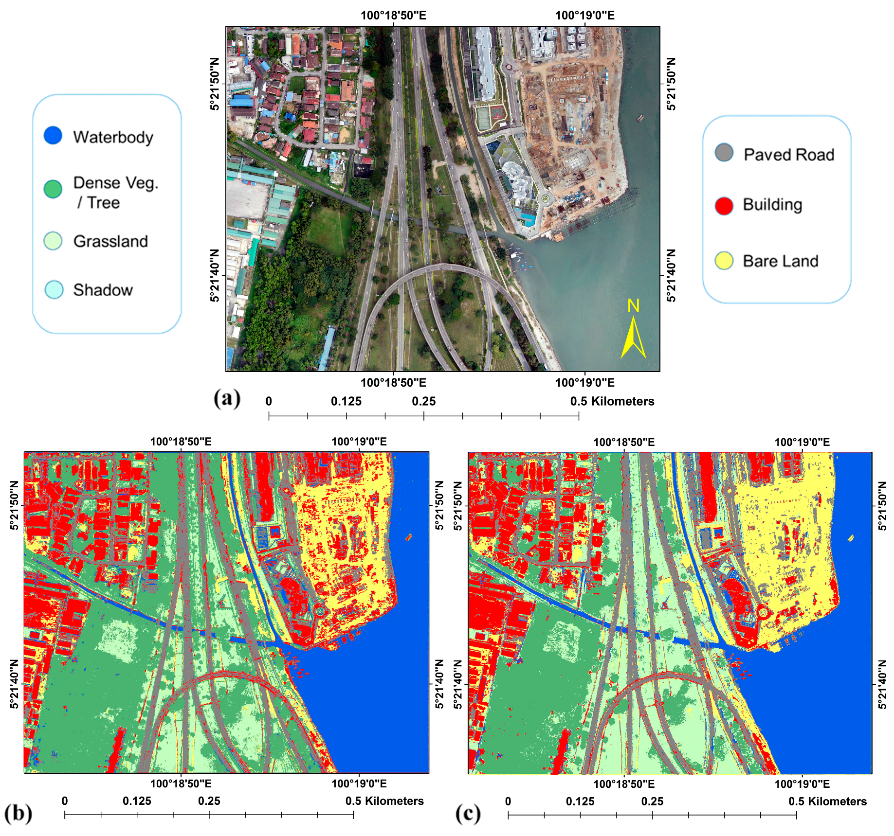
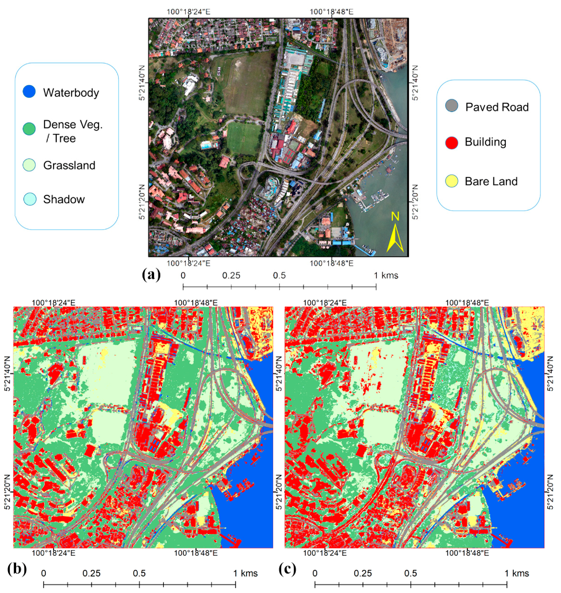
This section provides the experimental results of our study. The CNN was implemented in Python on an Intel Core-i7 (2.90 GHz) system with 32 GB RAM. The classification maps produced by CNN for both datasets are shown in Figure 3. The GT (Figure 3a) and the classified maps (Figure 3b,c) provided promising land cover classifications throughout the study area.

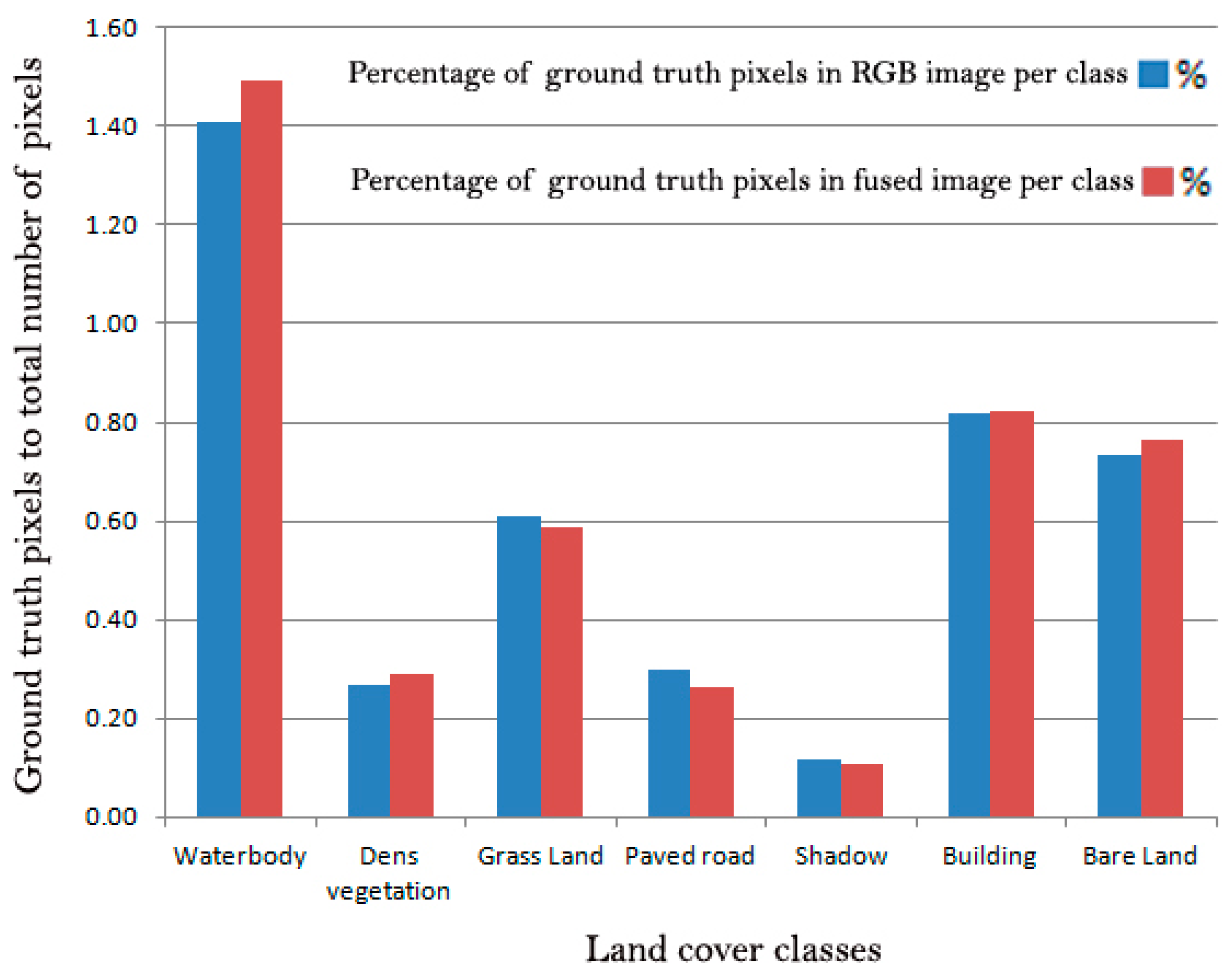
Figure 4 depicts the percentage of GT datasets pixels for each land cover class for both RGB and fused images. The GT samples in each class within the RGB image and the fused data were approximately balanced. Conversely, samplings between classes were not equally collected. For example, the number of GT pixels for the paved road classes in both datasets was approximately 0.3% while the percentages for the building class were close to 0.8%, which was nearly 2.6 times more sampling than for the paved road class. The percentage of GT pixels displayed variation from a minimum of 0.1% (in the shadow class) to a maximum of 1.5% (in the water body class). Therefore, the unbalanced distribution of GT samples between land cover classes resulted in obvious unfair distribution in training (50% of GT), validation (25% of GT), and testing (25% of GT) pixels, as well.

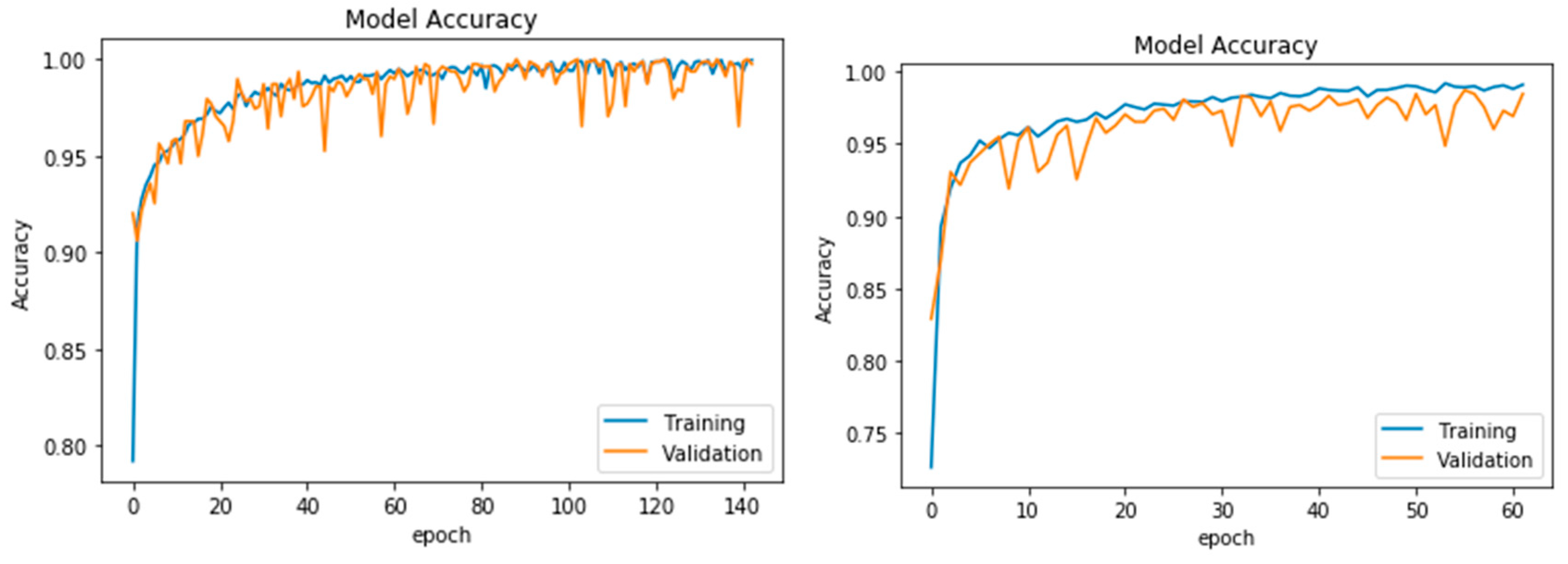
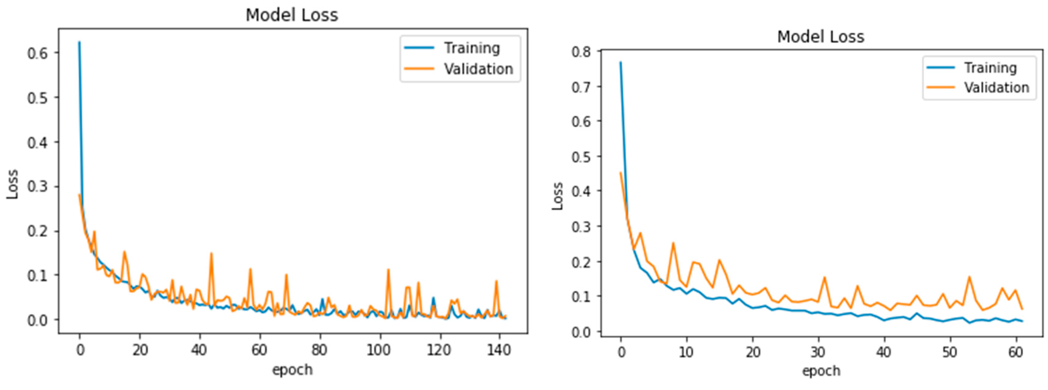
To evaluate the results, validation curves (accuracy and loss) of the two models are shown in Figure 5 and Figure 6. Figure 5 shows the accuracy curves (training and validation) for both datasets. Comparing the accuracies curves of the two methods, it is obvious that the two models were perfectly generalised, and that the validation accuracy curve is slightly higher than the training accuracy curve. Figure 6 represents the loss curves for the two CNN dataset classifiers. The loss of information in each model continued to decrease with training iteration for both methods. This pattern was also followed by the validation dataset.

Other evaluation metrics are presented in

Table 2. Performance of the classification methods used in the current study measured using standard accuracy metrics.

	Model	$\mathit{O}\mathit{A}$	$\mathit{A}\mathit{A}$	$\mathit{K}$
Training	CNN with DSM	0.991	0.989	0.988
	CNN without DSM	0.965	0.933	0.956
Testing	CNN with DSM	0.980	0.970	0.976
	CNN without DSM	0.968	0.952	0.961

OA = overall accuracy, AA = average accuracy, K = Kappa index

. The overall accuracy (OA) appeared to increase from 0.965 to 0.991 when the DSM image was considered. A similar improvement in the average accuracy (AA) was also recorded, from 0.933 to 0.989, when considering the DSM data. Similarly, the testing data (Table 2) showed an improvement in the OA from 0.968 to 0.980 and the AA improved from 0.952 to 0.970. Conversely, the highest value of the Kappa index (K) was measured (0.988) in the training data based on the implementation of the CNN with DSM. Undoubtedly, the model that did not include the DSM feature had a lower performance than the fused datasets using the testing and training datasets.

Table 3. Per-class accuracies (PA) for the training dataset.

Class	CNN with DSM	CNN without DSM
Bare land	0.996	0.981
Buildings	0.992	0.951
Dense vegetation	1.000	0.769
Grassland	0.956	0.946
Paved roads	0.990	0.995
Shadows	0.990	0.890
Water bodies	1.000	1.000

shows the per-class accuracies (PA) achieved by the proposed model based on the training data.

These results suggest that the CNN with DSM model was able to classify nearly all of the classes with relatively high accuracy. The maximum accuracy was 1.0 for the water body and dense vegetation classes, while the minimum accuracy belonged to the grassland class (0.956). Similarly, the maximum accuracy obtained by CNN without DSM was 1.0 for the water body class. Conversely, the minimum accuracy was obtained by the dense vegetation class at 0.769 for the CNN without DSM.

Table 4. PA obtained by the different classification methods for the testing dataset.

Class	CNN with DSM	CNN without DSM
Bare land	0.925	0.990
Buildings	0.983	0.979
Dense vegetation	0.966	0.923
Grassland	0.954	0.853
Paved roads	0.986	0.996
Shadows	0.978	0.923
Water bodies	0.999	0.999

shows that the additional DSM data improved the classification accuracy in the testing dataset compared to the RGB data alone. The highest PA recorded based on CNN with DSM was 0.999 referring to the water body class, and the lowest PA occurred in the bare land class with a value of 0.925. Conversely, the CNN without DSM (RGB only) had highest and lowest PA values of 0.996 (paved roads) and 0.853 (grassland).

Table 5. Recall, Precision, F1 Score obtained using CNN with DSM and CNN without DSM.

Class	CNN without DSM			CNN with DSM
	RecallMacro	PrecisionMacro	F1 ScoreMacro	RecallMacro	PrecisionMacro	F1 ScoreMacro
Bare land	0.976	0.998	0.987	0.959	1.00	0.979
Buildings	0.996	0.987	0.991	0.989	0.995	0.992
Dense vegetation	1.00	0.812	0.896	1.00	0.927	0.962
Grassland	0.872	1.00	0.931	0.954	1.00	0.976
Paved roads	0.966	0.975	0.971	0.995	0.946	0.970
Shadows	0.552	1.00	0.711	0.855	1.00	0.921
Water bodies	0.997	0.999	0.998	1.00	1.00	1.00

shows the Precision, Recall and F1 score for each class. The highest F1 score recorded based on CNN with DSM was 1.00 belonging to waterbody class, and the lowest F1 score referred to shadow class with a value of 0.921. Conversely, the CNN without DSM (RGB only) had the highest and lowest F1 score values of 0.998 and 0.711 by water body and shadow classes, respectively.

To further assess the performance and functionality of the proposed method, its transferability to another UAV subset was evaluated. The visual interpretation showed that the area consisted of several land cover types, including bare land, dense vegetation, grassland, waterbody, building, shadow, and paved road. The UAV was taken from the same environment to the first dataset, hence, the same set of hyperparameters was used for CNN (Activations = ReLU and Softmax, optimizer = Adam, batch size = 32, patch size = $9\times 9$, number of epochs = 200, and dropout = 0.2 and 0.5). Figure 7 shows the classified images obtained from the two datasets: (a) RGB only (b) fused RGB and DSM. The accuracy of the classification results is mentioned in

Table 6. Performance of the classification methods used in the current study measured using standard accuracy metrics.

	Model	$\mathit{O}\mathit{A}$	$\mathit{A}\mathit{A}$	$\mathit{K}$
Training	CNN with DSM	0.92	0.91	0.91
	CNN without DSM	0.89	0.86	0.88
Testing	CNN with DSM	0.90	0.89	0.89
	CNN without DSM	0.88	0.87	0.88

.

5. Discussion

The present study led to the generation of two land cover classification maps, as shown in Figure 3. According to a visual inspection, the bare land and buildings were misclassified more in the north-eastern part of the map based on the RGB image (Figure 3b) compared to the result based on the data fusion (Figure 3c). The additional elevation data points resulted in the better overall bare land classification, as seen in Figure 3c. A comparison between the classification results showed that more misclassifications were present when the DSM data were not considered in locations where there was confusion between grassland and dense vegetation areas. It is likely that the height data from the DSM allowed the network to correctly differentiate between grass and dense vegetation (trees).

Unexpectedly, despite including the DSM data, some paved roads were misclassified as buildings in the centre to south in Figure 3c. Both datasets performed well for water body classification. From these results, we hypothesise that the CNNs performed misclassifications primarily due to dataset imbalances, which is a point mentioned by Marcos et al. [14]. Lack of proper sampling could also be a contributing factor. Specifically, a majority of the sampled pixels was from water bodies (~1.5%); this class unsurprisingly had the best classification accuracy for both datasets. The smallest number of sampled GT pixels (Figure 4) was for the shadow, paved roads, and dense vegetation classes (less than 0.3%). Therefore, the homogeneity of the selected GT dataset between the land cover classes and fully representative sampling may increase the quality of CNN classification operations. These results show that the proposed CNN with DSM is an effective image classification approach and highlight the improved model performance compared to the CNN without DSM classifiers.

In addition, the accuracy curves (Figure 5) were used to qualitatively assess the results and indicated that there was no sign of overfitting in the processing and, therefore, using dropouts in the CNN process was a success. Likewise, the loss curves (Figure 6) for each model behaved uniformly and the appearance of the curves showed that the learning progress and the optimising process in both datasets were relatively good, as there were no plateaus in the curves [46], and the labelling improved during iteration [42,47]. This means that the optimisation process improved for several epochs and might suggest a comparably good performance of the model regularisation (dropout and batch normalisation) and optimisation algorithm (Adam optimiser), for both the CNN without DSM, and the CNN with DSM.

To confirm the success of setting the dropout, we carried on the whole experiments again, without setting dropout value in the process. The results of accuracy and loss curves (Figure 8 and Figure 9) showed that both model accuracy and model loss in validation dataset curves were associated with huge numerous fluctuations and plateaus. This behaviour in loss curves may suggest that model regularisation (without dropout) did not relatively improve within the iterations and it might affect the pixels labelling procedures. Validation curve showed variation from the actual label (i.e., training curve) and it fluctuated above the training curve, even though it finally decreased the loss of information, the curve was not as perfect as the previous experiment with dropout. Accuracy curves also showed unstable performance and they were lower than training curves especially in the RGB dataset, meaning that the model without dropout was not generalized as well as the model with setting dropout value. From those curves, it was concluded that removing the dropout had a more negative effect on the RGB dataset rather than the fused dataset.

According to the standard accuracy metrics (Table 2), it is obvious that the CNN performed better after fusing the DSM with the RGB image. Moreover, the PA value (Table 3) showed a high accuracy enhancement of up to 23.1% for dense vegetation, and 10% and 4.1% improvements for the shadow and building classes, respectively. This finding indicates that adding the height of the features (e.g., trees and buildings) to RGB images can improve the classification accuracy, especially in dense vegetation areas. Even though the PA value for paved roads showed a slight loss of accuracy (0.5%) for the CNN with DSM compared to the CNN without DSM and all the PA values for the other classes improved with respect to the fusion. Overall, the experimental results for both datasets indicate that the model architecture was appropriate. The best obtained values for the OA, AA, and Kappa index for the CNN with DSM for the training dataset were 99.1%, 98.8% and 98.8%, respectively, using UAV datasets with resolutions of 0.8 m/pixel.

6. Conclusions

UAV data were used to produce an RGB orthomosaic photo and a DSM of the study area. For this study, a deep-learning classifier (CNN) was used to exploit the two different datasets to map the existing land cover classes into bare land, buildings, dense vegetation (trees), grassland, paved roads, shadows, and water bodies: 1) a CNN was used to classify the orthomosaic photo data and 2) a CNN was used to classify the fused orthomosaic photo and DSM data. Both datasets resulted in an acceptable OA, AA, K and PA for the testing and training datasets. However, the dataset associated with the height information (the fused orthomosaic photo and DSM) performed better in most of the discriminative classes. In particular, where the appearances of objects are mostly similar and when there is no height information, a model can mistakenly categorise bare land as a building or classify grassland as trees (dense vegetation). Comparing the accuracies of the results between the CNN with DSM and CNN without DSM, OA, AA and K showed improvements of 2.6%, 5.6% and 3.2%, respectively, for the training dataset and 1.2%, 1.8% and 1.5% for the testing dataset. The use of DSM successfully enhanced the PA obtained for both the testing and training datasets. Nevertheless, our observations of paved road and building misclassifications imply that the CNN with DSM was sensitive to the training dataset and hyperparameters. Therefore, to enhance the results, additional GTs are needed according to the height differences for a specific object and discriminative class, as well as homogenised and well-distributed GT samples. This study showed the capability of CNN to accurately classify UAV images that have a lower resolution to compare with very-high resolution aerial photos, and it confirmed that the fusion of datasets is promising. Future work will focus on the sensitivity of CNNs with other fusion methods to the training dataset, regularisation functions and optimisers.

References

1. Lucieer, A.; Robinson, S.A.; Turner, D. Using an Unmanned Aerial Vehicle (UAV) for Ultra-High Resolution Mapping of Antarctic Moss Beds. In Proceedings of the 2010 Australasian Remote Sensing Photogrammetry Conference, Alice Springs, NT, Australia, 14–16 September 2010; pp. 1–12. [Google Scholar]
2. Al-Tahir, R.; Arthur, M. Unmanned Aerial Mapping Solution for Small Island Developing States. In Proceedings of the Global Geospatial Conference, Quebec City, QC, Canada, 14–17 May 2012; pp. 1–9. [Google Scholar]
3. Kalantar, B.; Halin, A.A.; Al-Najjar, H.A.H.; Mansor, S.; van Genderen, J.L.; Shafri, H.Z.M.; Zand, M. A Framework for Multiple Moving Objects Detection in Aerial Videos. In Spatial Modeling in GIS and R for Earth and Environmental Sciences; Elsevier: Amsterdam, The Netherlands, 2019; pp. 573–588. [Google Scholar]
4. Kalantar, B.; Mansor, S.B.; Halin, A.A.; Shafri, H.Z.M.; Zand, M. Multiple moving object detection from UAV videos using trajectories of matched regional adjacency graphs. IEEE Trans. Geosci. Remote Sens. 2017, 55, 5198–5213. [Google Scholar] [CrossRef]
5. Lelong, C.; Burger, P.; Jubelin, G.; Roux, B.; Labbé, S.; Baret, F. Assessment of unmanned aerial vehicles imagery for quantitative monitoring of wheat crop in small plots. Sensors 2008, 8, 3557–3585. [Google Scholar] [CrossRef] [PubMed]
6. Kalantar, B.; Mansor, S.B.; Sameen, M.I.; Pradhan, B.; Shafri, H.Z.M. Drone-based land-cover mapping using a fuzzy unordered rule induction algorithm integrated into object-based image analysis. Int. J. Remote Sens. 2017, 38, 2535–2556. [Google Scholar] [CrossRef]
7. Kalantar, B.; Mansor, S.; Halin, A.A.; Ueda, N.; Shafri, H.Z.M.; Zand, M. A graph-based approach for moving objects detection from UAV videos. Image Signal Process. Remote Sens. XXIV 2018, 10789, 107891Y. [Google Scholar]
8. Crommelinck, S.; Bennett, R.; Gerke, M.; Nex, F.; Yang, M.Y.; Vosselman, G. Review of automatic feature extraction from high-resolution optical sensor data for UAV-based cadastral mapping. Remote Sens. 2016, 8, 689. [Google Scholar] [CrossRef]
9. Ma, L.; Li, M.; Ma, X.; Cheng, L.; Du, P.; Liu, Y. A review of supervised object-based land-cover image classification. ISPRS J. Photogramm. Remote Sens. 2017, 130, 277–293. [Google Scholar] [CrossRef]
10. Liu, T.; Abd-Elrahman, A. An Object-Based Image Analysis Method for Enhancing Classification of Land Covers Using Fully Convolutional Networks and Multi-View Images of Small Unmanned Aerial System. Remote Sens. 2018, 10, 457. [Google Scholar] [CrossRef]
11. Jahan, F.; Zhou, J.; Awrangjeb, M.; Gao, Y. Fusion of Hyperspectral and LiDAR Data Using Discriminant Correlation Analysis for Land Cover Classification. IEEE J. Sel. Top. Appl. Earth Obs. Remote Sens. 2018, 99, 1–13. [Google Scholar] [CrossRef]
12. Gibril, M.B.A.; Bakar, S.A.; Yao, K.; Idrees, M.O.; Pradhan, B. Fusion of RADARSAT-2 and multispectral optical remote sensing data for LULC extraction in a tropical agricultural area. Geocarto Int. 2016, 1e14. [Google Scholar] [CrossRef]
13. Gomez-Chova, L.; Tuia, D.; Moser, G.; Camps-Valls, G. Multimodal classification of remote sensing images: A review and future directions. Proc. IEEE 2015, 103, 1560–1584. [Google Scholar] [CrossRef]
14. Marcos, D.; Volpi, M.; Kellenberger, B.; Tuia, D. Land cover mapping at very high resolution with rotation equivariant CNNs: Towards small yet accurate models. ISPRS J. Photogramm. Remote Sens. 2018, 145, 96–107. [Google Scholar] [CrossRef] [Green Version]
15. Irwin, K.; Beaulne, D.; Braun, A.; Fotopoulos, G. Fusion of SAR, optical imagery and airborne LiDAR for surface water detection. Remote Sens. 2017, 9, 890. [Google Scholar] [CrossRef]
16. Hartfield, K.A.; Landau, K.I.; van Leeuwen, W.J.D. Fusion of high resolution aerial multispectral and LiDAR data: Land cover in the context of urban mosquito habitat. Remote Sens. 2011, 3, 2364–2383. [Google Scholar] [CrossRef]
17. Zhu, X.; Cai, F.; Tian, J.; Williams, T. Spatiotemporal Fusion of Multisource Remote Sensing Data: Literature Survey, Taxonomy, Principles, Applications, and Future Directions. Remote Sens. 2018, 10, 527. [Google Scholar] [Green Version]
18. Sameen, M.I.; Pradhan, B.; Aziz, O.S. Classificationofveryhighresolutionaerialphotosusingspectral-spatial convolutional neural networks. J. Sens. 2018, 7195432. [Google Scholar]
19. Wang, Y.; Wang, Z. A survey of recent work on fine-grained image classification techniques. J. Vis. Commun. Image Represent. 2019, 59, 210–214. [Google Scholar] [CrossRef]
20. Feng, Q.; Liu, J.; Gong, J. UAV Remote sensing for urban vegetation mapping using Random Forest and texture analysis. Remote Sens. 2015, 7, 1074–1094. [Google Scholar] [CrossRef]
21. Gevaert, C.M.; Persello, C.; Vosselman, G. Optimizing multiple kernel learning for the classification of UAV data. Remote Sens. 2016, 8, 1025. [Google Scholar] [CrossRef]
22. Zhang, X.; Chen, G.; Wang, W.; Wang, Q.; Dai, F. Object-Based Land-Cover Supervised Classification for Very-High-Resolution UAV Images Using Stacked Denoising Autoencoders. IEEE J. Sel. Top. Appl. Earth Obs. Remote Sens. 2017, 10, 3373–3385. [Google Scholar] [CrossRef]
23. Gibril, M.B.A.; Idrees, M.O.; Yao, K.; Shafri, H.Z.M. Integrative image segmentation optimization and machine learning approach for high quality land-use and land-cover mapping using multisource remote sensing data. J. Appl. Remote Sens. 2018, 12, 016036. [Google Scholar] [CrossRef]
24. Gibril, M.B.A.; Shafri, H.Z.M.; Hamedianfar, A. New semi-automated mapping of asbestos cement roofs using rule-based object-based image analysis and Taguchi optimization technique from WorldView-2 images. Int. J. Remote Sens. 2017, 38, 467–491. [Google Scholar] [CrossRef]
25. Liu, T.; Abd-Elrahman, A. Multi-view object-based classification of wetland land covers using unmanned aircraft system images. Remote Sens. Environ. 2018, 216, 122–138. [Google Scholar] [CrossRef]
26. Liu, T.; Abd-Elrahman, A. Deep convolutional neural network training enrichment using multi-view object-based analysis of Unmanned Aerial systems imagery for wetlands classification. ISPRS J. Photogramm. Remote Sens. 2018, 139, 154–170. [Google Scholar] [CrossRef]
27. Liu, T.; Abd-Elrahman, A.; Zare, A.; Dewitt, B.A.; Flory, L.; Smith, S.E. A fully learnable context-driven object-based model for mapping land cover using multi-view data from unmanned aircraft systems. Remote Sens. Environ. 2018, 216, 328–344. [Google Scholar] [CrossRef]
28. Ma, L.; Fu, T.; Blaschke, T.; Li, M.; Tiede, D.; Zhou, Z.; Chen, D. Evaluation of Feature Selection Methods for Object-Based Land Cover Mapping of Unmanned Aerial Vehicle Imagery Using Random Forest and Support Vector Machine Classifiers. ISPRS Int. J. Geo Inf. 2017, 6, 51. [Google Scholar] [CrossRef]
29. Bergado, J.R.A.; Persello, C.; Gevaert, C. A Deep Learning Approach to the Classification of Sub-Decimeter Resolution Aerial Images. In Proceedings of the IEEE International Geoscience and Remote Sensing Symposium, Beijing, China, 10–15 July 2016; pp. 1516–1519. [Google Scholar]
30. Laliberte, A.S.; Goforth, M.A.; Steele, C.M.; Rango, A. Multispectral remote sensing from unmanned aircraft: Image processing workflows and applications for rangeland environments. Remote Sens. 2011, 3, 2529–2551. [Google Scholar] [CrossRef]
31. Zhu, X.X.; Tuia, D.; Mou, L.; Xia, G.S.; Zhang, L.; Xu, F.; Fraundorfer, F. Deep Learning in Remote Sensing: A Comprehensive Review and List of Resources. IEEE Geosci. Remote Sens. Mag. 2017, 5, 8–36. [Google Scholar] [CrossRef] [Green Version]
32. Guidici, D.; Clark, M.L. One-Dimensional convolutional neural network land-cover classification of multi-seasonal hyperspectral imagery in the San Francisco Bay Area, California. Remote Sens. 2017, 9, 629. [Google Scholar] [CrossRef]
33. Zhang, P.; Ke, Y.; Zhang, Z.; Wang, M.; Li, P.; Zhang, S. Urban Land Use and Land Cover Classification Using Novel Deep Learning Models Based on High Spatial Resolution Satellite Imagery. Sensors 2018, 18, 3717. [Google Scholar] [CrossRef] [PubMed]
34. Feng, Q.; Zhu, D.; Yang, J.; Li, B. Multisource Hyperspectral and LiDAR Data Fusion for Urban Land-Use Mapping based on a Modified Two-Branch Convolutional Neural Network. ISPRS Int. J. Geo Inf. 2019, 8, 28. [Google Scholar] [CrossRef]
35. Kussul, N.; Lavreniuk, M.; Skakun, S.; Shelestov, A. Deep learning classification of land cover and crop types using remote sensing data. IEEE Geosci. Remote Sens. Lett. 2017, 14, 778–782. [Google Scholar] [CrossRef]
36. Nahhas, F.H.; Shafri, H.Z.M.; Sameen, M.I.; Pradhan, B.; Mansor, S. Deep learning approach for building detection using liDAR-orthophoto fusion. J. Sens. 2018, 7212307. [Google Scholar] [CrossRef]
37. Zhu, Y.; Newsam, S. Land Use Classification Using Convolutional Neural Networks Applied to Ground-level Images. In Proceedings of the 23rd SIGSPATIAL International Conference on Advances in Geographic Information Systems, Seattle, WA, USA, 3–6 November 2015; pp. 1–61. [Google Scholar]
38. Liang, X.; Wang, X.; Lei, Z.; Liao, S.; Li, S.Z. Soft-Margin Softmax for Deep Classification. In International Conference on Neural Information Processing; Springer: Cham, Switzerland, 2017; pp. 413–421. [Google Scholar] [CrossRef]
39. Kingma, D.; Ba, J. Adam: A method for stochastic optimization. arXiv 2014, arXiv:1412.6980. [Google Scholar]
40. Ioffe, S.; Szegedy, C. Batch normalization: Accelerating deep network training by reducing internal covariate shift. arXiv 2015, arXiv:1502.03167. [Google Scholar]
41. Jmour, N.; Zayen, S.; Abdelkrim, A. Convolutional Neural Networks for Image Classification. In Proceedings of the International Conference on Advanced Systems and Electric Technologies (IC_ASET), Hammamet, Tunisia, 22–25 March 2018; pp. 397–402.
42. Mboga, N.; Persello, C.; Bergado, J.R.; Stein, A. Detection of Informal Settlements from VHR Images Using Convolutional Neural Networks. Remote Sens. 2017, 9, 1106. [Google Scholar] [CrossRef]
43. Zang, W.; Lin, J.; Zhang, B.; Tao, H.; Wang, Z. Line-Based registration for UAV remote sensing imagery of wide-spanning river basin. In Proceedings of the 19th International Conference on Geoinformatics, Shanghai, China, 24–26 June 2011; pp. 1–4. [Google Scholar]
44. Ramsey, E.W.; Jensen, J.R. Remote sensing of mangrove wetlands: Relating canopy spectra to site-specific data. Photogramm. Eng. Remote Sens. 1996, 62, 939. [Google Scholar]
45. Congalton, R.G. A review of assessing the accuracy of classifications of remotely sensed data. Remote Sens. Environ. 1991, 37, 35–46. [Google Scholar] [CrossRef]
46. Thoma, M. Analysis and optimization of convolutional neural network architectures. arXiv 2017, arXiv:1707.09725. [Google Scholar]
47. Abd, H.A.A.R.; Alnajjar, H.A. Maximum Likelihood for Land-Use/Land-Cover Mapping and Change Detection Using Landsat Satellite Images: A Case Study South of Johor. Int. J. Comput. Eng. Res. (IJCER) 2013, 3, 26–33. [Google Scholar]
48. Foody, G.M. Status of land cover classification accuracy assessment. Remote Sens. Environ. 2002, 80, 185–201. [Google Scholar] [CrossRef]
49. Cheng, H.; Lian, D.; Gao, S.; Geng, Y. Evaluating Capability of Deep Neural Networks for Image Classification via Information Plane. In Proceedings of the European Conference on Computer Vision (ECCV), Munich, Germany, 8–14 September 2018; pp. 168–182. [Google Scholar]
50. Tran, D.; Mac, H.; Tong, V.; Tran, H.A.; Nguyen, L.G. A LSTM based framework for handling multiclass imbalance in DGA botnet detection. Neurocomputing 2018, 275, 2401–2413. [Google Scholar] [CrossRef]
Figure 1. The unmanned aerial vehicle (UAV) datasets used in this work: (a) the orthomosaic image and (b) the constructed digital surface model (DSM).
Remotesensing 11 01461 g001
Figure 2. Flowchart of the proposed convolutional neural network (CNN) based classification model.
Remotesensing 11 01461 g002
Figure 3. Classification map produced by the CNN based on the two datasets: (a) GT, (b) RGB only dataset and (c) RGB + DSM dataset.
Remotesensing 11 01461 g003
Figure 4. Percentage and distribution of all GT to total classified pixels for each land cover class.
Remotesensing 11 01461 g004
Figure 5. Model accuracy when fusing DSM and RGB (left), and model accuracy with RGB only (right).
Remotesensing 11 01461 g005
Figure 6. Training and validation loss of information when fusing DSM and RGB (left), and loss of information with RGB only (right).
Remotesensing 11 01461 g006
Figure 7. Classification map produced by the CNN based on the two datasets: (a) GT, (b) RGB only dataset and (c) the RGB + DSM dataset.
Remotesensing 11 01461 g007
Figure 8. Training and validation accuracy curve without dropout when fusing DSM and RGB (left), and loss of information with RGB only (right) without dropout.
Remotesensing 11 01461 g008
Figure 9. Training and validation loss of information without dropout when fusing DSM and RGB (left), and loss of information with RGB only (right) without dropout.
Remotesensing 11 01461 g009