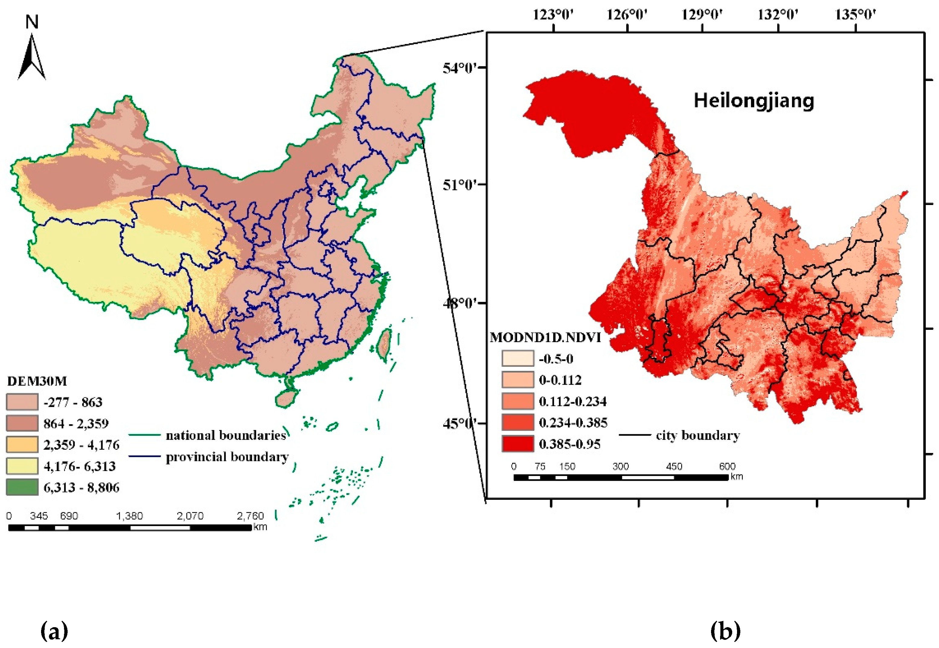
Article

Large-Scale Crop Mapping Based on Machine Learning and Parallel Computation with Grids

1
College of Land Science and Technology, China Agricultural University, Beijing 100083, China
2
Key Laboratory of Remote Sensing for Agri-Hazards, Ministry of Agriculture and Rural Affairs, Beijing 100083, China
3
Key Laboratory of Agricultural Land Quality and Monitoring, Ministry of Natural Resources, Beijing 100083, China
*
Author to whom correspondence should be addressed.
Remote Sens. 2019, 11(12), 1500; https://0-doi-org.brum.beds.ac.uk/10.3390/rs11121500
Submission received: 22 April 2019 / Revised: 21 June 2019 / Accepted: 21 June 2019 / Published: 25 June 2019

Abstract

:
Large-scale crop mapping provides important information in agricultural applications. However, it is a challenging task due to the inconsistent availability of remote sensing data caused by the irregular time series and limited coverage of the images, together with the low spatial resolution of the classification results. In this study, we proposed a new efficient method based on grids to address the inconsistent availability of the high-medium resolution images for large-scale crop classification. First, we proposed a method to block the remote sensing data into grids to solve the problem of temporal inconsistency. Then, a parallel computing technique was introduced to improve the calculation efficiency on the grid scale. Experiments were designed to evaluate the applicability of this method for different high-medium spatial resolution remote sensing images and different machine learning algorithms and to compare the results with the widely used nonparallel method. The computational experiments showed that the proposed method was successful at identifying large-scale crop distribution using common high-medium resolution remote sensing images (GF-1 WFV images and Sentinel-2) and common machine learning classifiers (the random forest algorithm and support vector machine). Finally, we mapped the croplands in Heilongjiang Province in 2015, 2016, 2017, which used a random forest classifier with the time series GF-1 WFV images spectral features, the enhanced vegetation index (EVI) and normalized difference water index (NDWI). Ultimately, the accuracy was assessed using a confusion matrix. The results showed that the classification accuracy reached 88%, 82%, and 85% in 2015, 2016, and 2017, respectively. In addition, with the help of parallel computing, the calculation speed was significantly improved by at least seven-fold. This indicates that using the grid framework to block the data for classification is feasible for crop mapping in large areas and has great application potential in the future.

Graphical Abstract

1. Introduction

The knowledge of croplands has important implications for food security, economic development, and agricultural policy making [1,2,3]. Crop-type mapping in large agricultural areas also provides important fundamental data for crop growth monitoring, yield estimation and drought warnings [4,5,6,7,8]. Traditionally, the crop-type information was obtained through field surveys, which are time- and labor-consuming. Remote sensing, either alone or in combination with statistical field statistical surveys, plays a key role in identifying and mapping croplands over large areas due to its synoptic view, multi-temporal coverage, and cost-effectiveness.
Agricultural applications require high accuracy, high spatial resolution and high update frequency large-scale crop classification products. However, mapping croplands over large areas with multi-spectral, multi-temporal remotely sensed data remains challenging due to the large volume of data caused by large area and the inconsistent of available imagery caused by cloudiness and uneven revisit times. A series of cloud computing platform were introduced, which greatly solving the calculation problem caused by a large volume of data [9,10,11,12,13]. In addition, both NASA’s NEX system for global processing and Infor Terra’s Pixel Factory for massive imagery auto processing use cluster-based platforms (a group of computers that are interconnected by a high-speed network) for calculation speed optimization [14,15]. However, due to the temporal inconsistency of image acquisition, there are still limitations in multi-temporal cropland classification [16,17,18,19,20,21,22], including (a) most of supervised classifiers require consistent number of features. [23,24,25]; (b) insufficient temporal information is used caused by the abandon of images acquired at a specific time without covering the full study area [9,26,27]. Thus, the overall accuracy of large scale cropland mapping is less than ideal (between 66% and 79%) [16,18,28,29]. Therefore, there remains a need to create better operational cropland map production based on high-medium resolution images (≤30 m) over large areas.
Many scholars have made efforts to solve the problem of inconsistent of available imagery. Some scholars have attempted to divide the study area into several small regions to ensure the same acquisition time of the images [30]. However, data scarcity in the time series is a common problem if the study area is too large, which could affect the classification accuracy. For instance, due to the influence of clouds and rainy weather, sufficient temporal information cannot be obtained [27]. Some methods have been proposed to compensate for the missing pixels, such as interpolation and resampling on time series [31], self-organizing Kohonen maps (SOMs), as well as extracting statistical values from time series [26,27]. However, the accuracy of the results obtained by these methods is still uncertain. To overcome these challenges, we focused on developing a framework based on grids to solve the problem of the inconsistent availability of remote sensing data and realize large-scale crop classification. Using grids to block the remote sensing data could reduce the data organization scale and maximize the use of the time series data to achieve better classification accuracy [17,21,32]. A set of unified encoding rules is a good way to optimize the computational speed required for processing massive remote sensing datasets with high-performance parallel computing.
Grids have been used in various application fields [33,34,35]. Ye et al. [36] designed a multilevel raster data cleaning and reconstitution multigrid (RDCRMG) system using universal transverse mercator projection (UTM projection). The RDCRMG system divides images into several consistent, independent blocks and distributed storage in different data. The raster data can be quickly extracted for the target areas by using the “no metadata” model, which directly calculates the data storage path without retrieving the metadata records. In addition, it allows the users to split the task into subtasks that can be executed in parallel. In large-scale crop classification, small-scale distributed storage makes it easier to obtain consistent time-series images. The no metadata concept applied with parallel computing can handle the calculation of massive raster datasets well. In this paper, we proposed a new workflow for large-scale crop mapping based on an RDCRMG from high-medium resolution images (≤30 m). Remote sensing data were clipped into the RDCRMG 10 km grid for unified management. Ten km grids were used as the calculation unit for classification, which means that the classification model was trained in each grid independently, and the temporal features were generated from the images in each grid.
In summary, to cope with the inconsistent availability of high-medium resolution images (≤30 m) over large-scale cropland mapping, we proposed a new efficient and effective workflow based on RDCRMG. First, we used the 10 km grid as the basic processing unit and classified images in each grid with the whole samples but different temporal features according to the GF-1 revisit times in this grid. Secondly, we designed a parallel computing approach based on a 10 km grid and integrated a machine learning algorithm, which greatly improved the calculation speed without sacrificing classification accuracy. The workflow was applied to the classification of Heilongjiang Province, which is the highest food-producing province and covers a 4.73 Mha area in China, with GF-1 WFV images and random forest classifier.

2. Materials

2.1. Study Area

Heilongjiang Province, which is located in the northeastern part of China between 43°26′N–53°33′N and 121°11′E~135°05′E (Figure 1), is an important commodity base for grain in China. From south to north, according to temperature indicators, Heilongjiang can be divided into a medium temperature zone and a cold temperate zone. From east to west, according to the dryness index, it can be divided into a wet zone, a semi-humid zone, and a semiarid zone. Covering an area of 4.73 Mha, the terrain is roughly high in the northwest, north, and southeast and low in the northeast and southwest. There are approximately 1.18 Mha of cultivated agricultural land, accounting for 30% of the total land. The major crops are corn, rice, and soybeans. They are all sown at May and harvested in late September. The annual average rainfall of Heilongjiang is 400–700 mm, of which 60% is concentrated from June to August.

2.2. Data Sources and Preprocessing

2.2.1. Remote Sensing Data

The Gaofen-1 (GF-1) WFV imagery was utilized in this study due to its high spatial and temporal resolution. The GF-1 satellite was launched on 26 April 2013 and is the first satellite in the civilian high-definition earth observation satellite (HDEOS) program to realize a high-resolution and wide-swath optical remote sensing mission. It has two high-spatial-resolution cameras and four wide field viewing cameras with a combined width of 800 km. The GF-1 satellite has a spatial resolution of 16 m and four spectral bands: blue (0.45–0.53 μm), green (0.52–0.59 μm), red (0.63–0.69 μm), and near-infrared (0.77–0.89 μm). Its temporal resolution is 2 days. GF1 WFV imagery have been widely used in crop classification, in-season crop mapping, crop planting area survey etc., and has achieved good results [37,38,39]. The GF-1 satellite data can cover the whole world, and it has the most abundant temporal data and the most comprehensive coverage over China. The data can be downloaded from the official website of the China Resources Satellite Application Center [40]. Organizations need to register an account on the website and apply for subscription rights. The GF-1 images can be downloaded for free if permission is granted.
The GF-1 satellite has 8-track imaging and 35° imaging capability per side. We downloaded the images from May to September for classification, with a total of 742 scenes in 2015, 462 scenes in 2016, and 571 scenes in 2017. To ensure the quality of the classification, we only used the images with less than 10% cloud cover. Following these rules, the GF-1 WFV sensor acquired a total of 398 scene images in 2015, 291 in 2016, and 272 in 2017 covering Heilongjiang Province. Figure 2 shows the detailed temporal distribution.

2.2.2. Field Sample Data

The field sample data provide a basic reference for crop classification. We randomly sampled the data according to the size of the study area, distribution of the major crops and accessibility to the field sites. Corn is widely distributed mainly in the central, western, and southern regions of the province due to economic factors. Rice is mainly distributed in the Sanjiang Plain and along the river region. Soybeans are mainly distributed in the central and northern parts. Figure 3 shows the distribution of crops.
In addition to these three crops, we also collected samples of wheat, woods, greenhouses, buildings, water, etc., but because these land cover types are not our main focus and the number is small, when performing the classification, they are merged into a single class named “other”. According to the actual sampling plan, we randomly selected 2235 corn samples, 639 rice samples, 1308 soybean samples, and 765 other samples each year and divided it into the training data and test data at a ratio of 2:1.

2.2.3. RDCRMG and Automated Preprocessing System

Raster dataset clean and reconstitution multigrid (RDCRMG) is a multisource raster data organization and management logic framework that is similar to the Military Grid Reference System (MGRS) data organization framework. Currently, the implementation of RDCRMG is mainly based on code and includes some basic functionality based on the graphical user interface (GUI), such as the preprocessor. According to the RDCRMG system, three levels of square grids (100 km–10 km–1 km) with different grid sizes, strictly nested relationships, and specific codes are used as consistent RS image partition units. It includes the UTM 6° band–100 km grid–10 km grid–time–data type encoding rules, and we used a 10 km grid as our data organization unit. In the RDCRMG system, the grid codes are used as the directory name and file name to generate the logical storage paths of the raster file blocks based on the “no metadata” model, as shown in Figure 4.
The GF-1 WFV data used in this paper needed to undergo the following preprocessing steps before being entered into the RDCRMG: metadata reading, radiometric calibration, atmospheric correction, orthorectification, cloud detection, geometric registration, projection conversion, clipping, and cleaning [36]. Figure 5 shows the temporal data of the grid after the image is entered into the RDCRMG. The sample data in the RDCRMG underwent the following steps: rasterization, metadata reading, project conversion, cropping, and cleaning. Figure 6 shows the number of samples in each grid unit after the sample was entered into the RDCRMG system.

2.3. Spectral Features

To maximize the differences among rice, corn, and soybeans, we not only use the original spectral values as features but also calculate the enhanced vegetable index (EVI) [41] and the normalized difference water index (NDWI) [42].
The EVI was proposed by Huete et al. [41] and is one of the most widely used vegetation indices. It can effectively reflect the vegetation coverage and eliminate the influence of the atmosphere. In addition, it has a good correlation with the vegetation coverage that does not easily reach saturation. Studies have shown that the EVI can effectively reflect the physiological characteristics of different crops in different growing seasons at different growth stages [32]; the calculation formula is as follows:
E V I = 2.5 ( N I R R E D ) / ( N I R + 6 R E D 7.5 B L U E + 1 )
The NDWI, proposed by Mcfeethers [42], minimizes the vegetation information and highlights the water information. It is sensitive to changes in the liquid water content of the vegetation canopy. Yang et al. used it to extract rice information and achieved good results [43]. The NDWI is calculated as follows:
N D W I = ( G R E E N N I R ) / ( G R E E N + N I R )
The temporal profile of various crops is shown in Figure 7. The corn, rice, and soybeans are sown at the end of April and harvested in September, so the feature trends of these three crops are basically the same. On day of the year (DOY) 130, the surface of the rice field is covered by water, and the soybean has an obvious texture when it is just planted. Therefore, in the red and green bands, the rice has the lowest spectral value. On DOY 156, the soybean is flowering; the corn is in the seventh leaf stage; and the rice is in the stage of greening and tillering, so the rice has a higher NDWI value. Between DOY 220 and 240, the differences in the NIR and EVI values among the corn, rice, and soybean are obvious, all of them reached their peaks, and they were significantly different. During the harvest period, the features of the three crops also behave differently.

3. Method

Our approach for large-scale crop mapping based on high-medium resolution images involved four steps: (1) feeding both the images and sample data into the RDCRMG grid system; (2) selecting high-quality images and reconstructed a sample dataset with all ground truth sample locations and with full temporal profile, then calculated features; (3) generating the training data and test data according to a 2:1 ratio and (4) extracting a training features dataset based on the dates of the satellite revisited for each 10 km grid, then optimizing hyperparameters and classifying. Next, all the classification results were mosaicked into one entire crop type map, and the test data were used for an accuracy assessment based on the confusion matrix. We employed the parallel computing strategy in the second and fourth steps. This also means that we generated 4951 predictive models. Since Heilongjiang study area covers 4951 10 km grids, the grids with the same temporal images were predicted using the same model. Figure 8 shows the detailed classification procedure. The whole workflow was implemented using the C# language, and the classifier was implemented with the Python scikit-learn package [44]. We established a grid attribute table in an Oracle database, which contains all the grids in Heilongjiang study area. The specific fields include ISINCLDSAMPLE (whether there are samples), ISINCLDIMG (whether there are images), and CLASSRLT (whether there are classification results) to indicate the progress of the classification. For example, before the second step, all the fields of all the grids were marked as pending. After the third step, the training and test data are all generated, and the ISINCLDSAMPLE and ISINCLDIMG fields are marked as completed. The program automatically monitors these unprocessed grids until all the steps for all the grids have been completed.

3.1. Image Selection

To ensure the quality of the classification, the images were carefully selected based on the amount of cloud coverage and image coverage for the following three scenarios: (i) Image mosaic. For example, if there were two GF-1 WFV images, a and b, which were adjacent to each other, the two scenes were merged.
(ii) Cloudless image selection. When downloading a high-resolution WFV image, we only downloaded the images of the entire scene with a cloud content below 10%. The impact of the cloud coverage on the classification results is very large, so before the classification, to ensure the quality of the results, we again filtered the data in 10 km grid units. At this time, only the 10 km grid raster images with cloud content below 60% were selected for classification. (iii) Large image selection. It was found that if the image did not cover the entire grid, there were obvious edge effects in the classification results. Therefore, we only used the images in which the imaging area occupied more than 75% of the 10 km grid area. Figure 9 shows the data acquisition scenarios and the amount of data in the 10 km grid after the image acquisition.

3.2. Full Temporal Profile Reconstruction

The difficulties of large scale multi-temporal classification are: (a) not every grid contains ground truth sample locations, (b) not every grid contains samples of all crop types, and (c) the dates of images covering each grid may largely differ. Therefore, we reconstructed a training sample dataset with all ground truth sample locations and with full temporal profile (containing the union of all observation time points of GF-1 satellite in whole study area), as shown in Figure 10.
In the process of reconstructing the full temporal profile for each sample location, we used linear interpolation to fill in the missing spectral values according to the images before and after. For each time point in the temporal profile, we prepared six features including four spectral bands, EVI and NDWI.

3.3. Training and Classification

We trained different models separately for each 10 km grid, using all sample locations in our training dataset but with different features according to the actual image availability of each grid. By this approach, even if there is no sample location in a specific grid, we still have the whole sample locations to use for training, by simply filtering the features according to the availability of temporal images in this grid, as shown in Figure 10. For example, if a grid contained images acquired on May 1 and June 1, we used only features of these two dates by extracting the corresponding feature columns from the training data table of all sample locations for training. Then, classification was done with the available images of this 10 km grid using the trained classifier. We integrated Scikit-learn [45] in Python in our classification framework for training and classification, and optimized the parameters by gridsearchcv function of this package to reach a better choice of the hyperparameters.

3.4. Parallel Computing

The RDCRMG retrieval strategy adopted the concept of the map-reduce mode. Based on this, a parallel strategy was implemented for the classification. By calculating the corresponding 10 km grid codes of the query scope, the calculation of each grid was performed in parallel. In addition to acquiring the union of all observation time points of GF-1 satellite in whole study area and generating the training sample dataset with all ground truth sample locations and with full temporal profile, all the remaining steps could be performed in parallel.
Parallel computing was implemented at both the thread and process levels and was based on a computing cluster of four servers. The machine parameters are shown in Table 1. First, the program was connected to the Oracle database, the field information was read in the grid attribute table, and then a pending grid set was assigned to each process. Second, in each process, the grid subset encoding sequence was assigned to each thread to implement thread-level parallel computing. Each thread allocation node would design a different number of threads according to the calculated required memory to prevent a computer memory overflow. The experiment showed that under the given computational resources, we could simultaneously perform the calculations for 18 grids.

3.5. Method Performance Evaluation

We evaluated the performance of this method in three different ways as follows:
First, we assessed the applicability of the method with different machine learning classifiers and remote sensing images. In terms of the classifiers, we chose the random forest classifiers and support vector machines. The random forest (RF) algorithm is a widely used machine learning method based on decision trees. Bootstrap sampling was used to train each decision tree, and the results yielded by the random forest algorithm were determined by the output of all the decision trees involved [45,46,47,48]. The support vector machine (SVM) classifier was derived from statistical learning theory. The training samples are segmented by a hyperplane. The principle of segmentation aims to maximize the interval and finally transform it into a convex quadratic programming problem [49,50]. The specific parameter values set when the two classifiers perform hyperparameter optimization are shown in Table 2. In terms of the data, in addition to the GF-1 WFV images, we used the sentinel 2 images in a small research area and compared the classification results with the classification results based on GF-1 WFV images.
Second, we selected a small study area and applied the widely used nonparallel classification methods for the classification and then compared the performance. There are two differences between our method and the widely used nonparallel methods. The first is that we classified by 10 km grid units, and for each grid, the available images of all the dates during the crop phenology were used as much as possible. Second, we used the temporal resampling to supplementary time series image for the grids with samples.
The third evaluation approach is to verify the migration of the classification model within the study area. Because the study area is large, we used the whole samples to classify and did not consider the inconsistent characteristic curves among crops in different regions. So, we divided the study area into two parts, one for the southwestern region where samples are scarce, labeled A, and the northeastern region labeled B. Two-thirds of the samples from B were used for training, and A/B was classified to use this model. Finally, the classification accuracy of A/B was compared.

3.6. Efficiency Test

To determine how much the efficiency of parallel classification can be improved, two models were used to determine the classification speed with the same grids (Figure 11). Certain grids with and without samples were selected for classification using the speed test. For mode 1, we used a parallel classification technique proposed in this paper, which was carried out with multi-process and multithread parallel computing. For mode 2, the classification was executed in one single thread.

3.7. Heilongjiang Classification Results Accuracy Assessment

The classification results for Heilongjiang study area were evaluated in two different ways. First, a confusion matrix was used for the accuracy assessment. The following metrics were calculated: the overall accuracy, average accuracy of the map, and the user and producer accuracy of each type of crop. The second evaluation method was to compare the area and interannual variation of the three main crops, which were analyzed separately. At the same time, the relevant policies promulgated by the Chinese government and statistical data were used as an aid to analyze the influencing factors.

4. Results

4.1. Results of the Accuracy Assessment

4.1.1. Verification of the Suitability of the Method

We assessed the applicability of the proposed method in terms of the classifiers and images. Table 3 shows the comparison results of the random forest and the support vector machine algorithms. They both achieved good results, and the accuracy is almost the same. Therefore, the computational framework proposed in this paper is applicable to a general machine learning classification algorithm based on supervised classification.
Our method can also be applied to the Sentinel-2 data. In the small study area, the classification result derived from the Sentinel-2 data had an average classification accuracy of 83% and an overall classification accuracy of 77%. Furthermore, the results showed that the use of the GF-1 WFV images had a higher overall accuracy compared with using the Sentinel-2 images (Table 4). The OA increased by 6% when using the GF-1 WFV images. Because the 2017 Sentinel-2B data are still in the testing stage, and a time resolution of 5 days has not yet been fully achieved. Therefore, the temporal information from the GF-1 WFV images was relatively richer than that of the Sentinel-2 images, which could distinguish different crops more accurately.

4.1.2. Accuracy Comparison with the Widely Used Classification Method

The results of our proposed classification method and the widely used nonparallel classification method were very similar. We selected a sample grid from the 32,653 projection tape as the experimental area. Experiment I used the proposed algorithm, and Experiment II used the widely used method. Before the classification, we simulated the common large-scale classification database and rules were as follows: (i) ensure that no single-date data can cover the entire research area; (ii) the image set in the experimental area has an irregular time series. Table 5 shows a comparison of the classification results. The overall accuracy and average accuracy of Experiments I and II were equal, however, the classification accuracy of different crops was different. The accuracy of rice obtained by the proposed method was significantly higher than that of the traditional method. The reason is that our method could make full use of the crop time series characteristics, which is beneficial for rice identification.

4.1.3. Assessment of the Classification Model Migration

The classification accuracy of the grids that were far from the sample collection area did not decrease. The results showed that the classification accuracy from the 256 test samples in Region-A was 80%, while the accuracy from the 1000 test samples in Region-B was 83%. Therefore, we believe that the proposed method is not sensitive to the differences between crops from different regions of Heilongjiang Province.

4.2. Computation Performance Evaluation

We set up six groups of experimental data, and each group had a different number of grids as follows: 18, 90, 180, 270, 360, and 450 grids. In each group, one half of the grids contain samples and the other half not contain samples. A task-level parallel computing cluster with four spatial analysis servers and one load-balancing server was deployed as the infrastructure for the efficiency tests. For mode 1, each grid was classified in parallel, and 18 grids at a time were calculated. For mode 2, the widely used methods were used to classify the grids one at a time. Figure 12 presents the time consumption for the classification of modes 1 and 2 with different sized query scopes. It can be seen that parallel computing based on RDCRMG can significantly improve the computational efficiency by approximately seven times, and the improvement is more obvious as the number of computing grids increases.

4.3. Heilongjiang Province Classification Results

Although the classification accuracies of the random forest and the support vector machine classifiers were almost the same, when the random forest classifier generated a decision tree, each node was generated from the optimal segmentation of several randomly selected variables, which we believe helped find the best sample set for each grid to classify. Finally, we chose the random forest classifier for the three-year classification of Heilongjiang Province. The results showed that the proposed method demonstrated a good performance for cropland mapping in the study area. Figure 13 indicates that the corn was distributed in most parts of the province and it cultivation area was large.
Rice was concentrated in the eastern region, while soybeans were mainly distributed in the north-central region, and the rice and soybean areas were relatively small and clustered. A few regional subsets of the crop maps are shown in Figure 14.
From 2015 to 2017, corn acreage has been decreasing, and rice and soybean acreage has been growing. After consulting the relevant data, it was found that, since the implementation of the corn reserve policy in China in 2008, the corn planting area in Heilongjiang Province has increased from 0.38 Mha to more than 6.7 Mha. The price of corn has been falling and the cost of storage has been high. Therefore, starting in 2015, China reformed the corn storage system and increased the subsidies for corn, but reduced the corn planting area. At the same time, the area planted with rice and soybeans has been growing, and soybeans have increased even more. Since 2016, China has carried out pilot work on the arable land rotation system, and selected seven cities in Heilongjiang to carry out pilot work, which has encouraged some growers to rotate crops to plant soybeans, so the soybean planting area has increased. In 2017, Heilongjiang Province vigorously promoted the “dry to water” policy, which meant changing low-lying land and saline-alkaline land into fertilizer fields. Therefore, the rice planting areas in the Sanjiang Plain and Songhua River Basin increased significantly. Overall, the classification results of this paper are consistent with the adjustment trend of the agricultural planting structure in Heilongjiang Province.
The classification accuracy of each crop type over three years is shown in Table 6. The user accuracy (UA) of the corn was the highest. However, the producer accuracy (PA) of the corn in 2016 and 2017 was lower, and the rice and soybeans were largely misclassified as corn, indicating that the sample size of the corn was too large. The PA of rice was the highest, partly because the characteristics of water (the growing environment of rice) were clearly reflected in the spectral values of the EVI and NDWI. Both the soybean UA and PA were high except in 2016. We can see that the mixed phenomenon of the soybean and corn was the most serious in 2016, partly because the time series features were not able to distinguish the corn and soybean very well.
In order to further verify the method proposed in this paper, we use a leave one year out verification method to classify and verify the Heilongjiang Province results based on GF-1 WFV data. We set up three sets of experiments, respectively: (i) we used sample locations of 2015 and 2016 to train the model. Then, this model was used to classify 2017, and sample locations from 2017 were used to evaluate the accuracy; (ii) we used sample locations of 2015 and 2017 to train the model. Then, this model was used to classify 2016, and sample locations of 2016 was used to evaluate the accuracy. (iii) train the time series spectral values of all samples in 2016 and 2017 to classify the 2016 data and use the 2015 test samples for accuracy assessment. Because the footprints of the GF-1 satellite do not overlap during three years, we select one image every half month as a representative image of this growth period, and select nine images every year, thus ensuring the consistency of the three-year time series features. The classification accuracy are shown as Table 7. We can see that it is not satisfactory. The reasons are as follows: (i) the spectral difference of GF-1 WFV data in different years is too large, and it is not suitable for classification with spectra of other years; (ii) the method we proposed that training and classification based on the actual image availability of each 10 km grid can better solve the irregular irregularity of the GF-1 satellite’s footprints.

5. Discussion

5.1. Reliability of Large Area Crop Mapping Using the Proposed Method

Currently, large-scale crop mapping based on high-medium spatial resolution (≤30 m) images still faces great challenges, mainly due to inconsistent availability of data. At present, there are two main methods for large-scale cropland mapping: (1) constructing a large sample set of all the land cover classes (cropland is one of them), which is time- and labor-consuming and difficult to repeat; or (2) replace the time series data with statistical data, for example, replacing the enhanced vegetation index (EVI) time series with the temporal EVI statistics, such as the mean, standard deviation, and maximum EVI. Our research proposes a new method for large-scale crop mapping by partitioning the study area and using parallel computing based on RDCRMG. The 10 km RDCRMG grids are used as a classification unit to ensure that the time series images are consistent, and it is also used as the calculation unit to design the parallel calculations to improve the classification speed.
The proposed method is applicable to all the remote sensing data under WGS 84 coordinates based on machine learning classifiers, and the accuracy achieved by the widely used nonparallel method was basically consistent with that achieved by our method. Even the inconsistent characteristic curves among crops in different regions, but it is not sensitive for this method in Heilongjiang. We then verified the efficiency improvement of the proposed calculation method. Compared with the traditional single-threaded classification, parallel classification can significantly improve the calculation speed, which is approximately seven times higher. The larger the number of grids is, the more obviously the speed improves by parallel classification. This provides a good solution for the calculation of larger areas.

5.2. Evaluation of Classification Results in Heilongjiang Province

In the classification results of the Heilongjiang study area, the geographic distribution of various crops is consistent with the actual statistics. Corn is widely distributed throughout the province, rice cultivation is concentrated in the eastern region, which is located in the Sanjiang Plain and is rich in water resources and soybeans are mainly distributed in the central and northern regions. The overall accuracy over the three years is between 81% and 88%. This result can already be used as a mask layer in the yield forecast model. However, due to the relatively low number of samples, the phenomena of the rice and soybean being misclassified into corn is more serious. Although there are enough samples of the corn, the mixed phenomenon of the corn and soybean still exists, so it may be necessary to increase samples and try to balance the samples of crops to be classified in a future study.
To ensure China’s food security, the Heilongjiang government has introduced a number of policies for the corresponding counties. In 2015, the government has reduced corn acreage and encouraged corn and soybean crop rotation, so the area planted with corn has been falling. In 2016, China’s corn prices fell, while the soybean prices rose, and farmers were encouraged to grow soybeans to reduce the soybean imports. The soybean planting area increased significantly in 2017 compared with the area in 2016. In the same year, the proposal of the drought-to-water policy greatly increased the area planted with rice.
In addition to these three major crops, we also analyzed the accuracy of other types of land cover, including natural vegetation, metropolitan areas and water. Natural vegetation, such as forests, has an accuracy of approximately 81%. Metropolitan areas, such as residential areas, have an accuracy of approximately 98%, and water, such as rivers, have an accuracy of approximately 99%. The classification results are shown in Figure 15. Although we mainly identify corn, rice and soybeans, the methods proposed in this paper can recognize other common land cover categories well.

5.3. Uncertainty Analysis and Outlook

There are some cases in which the classification accuracy of the proposed method is uncertain: (i) The more high-quality images there are, the better the classification accuracy will be, so integrating more images from different sources in the RDCRMG system will improve the classification results in the future. (ii) The remote sensing images should be as close as possible to the WGS-84 coordinates; otherwise, the classification result may have a large positional shift. (iii) Although we verified that the distance from the sample cluster is not related to the classification accuracy, a wide coverage and a large number of sample sets are more favorable for a higher accuracy.

6. Conclusions

Based on the RDCRMG grid, we proposed an efficient method to solve the inconsistent availability of data for large-scale cropping mapping. The proposed method can quickly and accurately distinguish among different crop types based on high-medium resolution images in large area. Using this approach, a crop classification was performed for Heilongjiang Province from 2015 to 2017 with a random forest classifier and GF-1 WFV images. The classification accuracy reached 88%, 82%, and 85% in 2015, 2016, and 2017, respectively, and the crop distribution was consistent with the government-promulgated policy. The entire classification process was completed within 22 hours to generate a cropland map of 4.73 Mha. Parallel computing was applied to the crop classification, which increased the computational efficiency by approximately seven times. The larger the study area is, the faster the speed is that can be realized.

Author Contributions

J.H. and D.Z. designed the study. N.Y., D.L., T.R. designed, implemented, and validated the method. N.Y., Q.F., J.H. and Y.Z. designed, completed, and revised the manuscript. Q.X. and L.Z. completed remote sensing data and sample preprocessing. J.H. and D.Z. gave technical support. The final draft was read and approved by all authors.

Funding

This research was funded by the National Nature Science Foundation of China, grant numbers 41671418; the Fundamental Research Funds for the Chinese Central Universities, grant numbers 2019TC117; the Science and Technology Facilities Council of UK- Newton Agritech Programme, grant number ST/N006798/1; the Foundation for Key Program of Beijing, grant number D171100002317002; and the China Postdoctoral Science Foundation, grant number 2018M641529, 2019T120155.

Acknowledgments

The authors would like to thank Cong Ou and Wen Zhuo for their suggestions in improving both the structure and the details of this paper.

Conflicts of Interest

The authors declare no conflict of interest.

References

  1. Huang, J.; Ma, H.; Sedano, F.; Lewis, P.; Liang, S.; Wu, Q.; Su, W.; Zhang, X.; Zhu, D. Evaluation of regional estimates of winter wheat yield by assimilating three remotely sensed reflectance datasets into the coupled WOFOST–PROSAIL model. Eur. J. Agron. 2019, 102, 1–13. [Google Scholar] [CrossRef]
  2. Huang, J.; Sedano, F.; Huang, Y.; Ma, H.; Li, X.; Liang, S.; Tian, L.; Zhang, X.; Fan, J.; Wu, W. Assimilating a synthetic Kalman filter leaf area index series into the WOFOST model to improve regional winter wheat yield estimation. Agric. For. Meteorol. 2016, 216, 188–202. [Google Scholar] [CrossRef]
  3. Huang, J.; Tian, L.; Liang, S.; Ma, H.; Becker-Reshef, I.; Huang, Y.; Su, W.; Zhang, X.; Zhu, D.; Wu, W. Improving winter wheat yield estimation by assimilation of the leaf area index from Landsat TM and MODIS data into the WOFOST model. Agric. For. Meteorol. 2015, 204, 106–121. [Google Scholar] [CrossRef] [Green Version]
  4. Lambin, E.; Meyfroidt, P. Global land use change, economic globalization, and the looming land scarcity. Proc. Natl. Acad. Sci. USA 2011, 108, 3465–3472. [Google Scholar] [CrossRef] [PubMed] [Green Version]
  5. Thenkabail, P.; Wu, Z. An Automated Cropland Classification Algorithm (ACCA) for Tajikistan by Combining Landsat, MODIS, and Secondary Data. Remote Sens. 2012, 4, 2890–2918. [Google Scholar] [CrossRef] [Green Version]
  6. See, L.; Fritz, S.; You, L.; Ramankutty, N.; Herrero, M.; Justice, C.; Becker-Reshef, I.; Thornton, P.; Erb, K.; Gong, P.; et al. Improved global cropland data as an essential ingredient for food security. Glob. Food Secur. 2015, 4, 37–45. [Google Scholar] [CrossRef]
  7. Huang, J.; Gómez-Dans, J.; Huang, H.; Ma, H.; Wu, Q.; Lewis, P.; Liang, S.; Chen, Z.; Xue, J.; Wu, Y.; et al. Assimilation of remote sensing into crop growth models: Current status and perspectives. Agric. For. Meteorol. 2019, 276-277C, 107609. [Google Scholar] [CrossRef]
  8. Huang, J.; Ma, H.; Su, W.; Zhang, X.; Huang, Y.; Fan, J.; Wu, W. Jointly assimilating MODIS LAI and ET products into the SWAP model for winter wheat yield estimation. IEEE J. Sel. Top. Appl. Earth Obs. Remote Sens. 2015, 8, 4060–4071. [Google Scholar] [CrossRef]
  9. Tian, F.; Wu, B.; Zeng, H.; Zeng, H.; Zhang, X.; Xu, J. Efficient Identification of Corn Cultivation Area with Multitemporal Synthetic Aperture Radar and Optical Images in the Google Earth Engine Cloud Platform. Remote Sens. 2019, 11, 629. [Google Scholar] [CrossRef]
  10. Dong, J.; Xiao, X.; Menarguez, M.; Zhang, G.; Qin, Y.; Thau, D.; Biradar, B. Mapping paddy rice planting area in northeastern Asia with Landsat 8 images, phenology-based algorithm and Google Earth Engine. Remote Sens. Environ. 2016, 185, 142–154. [Google Scholar] [CrossRef] [Green Version]
  11. Li, Z.; Wu, B.; Gommes, R.; Zhang, M.; Chen, B. Design framework for CropWatch Cloud. J. Remote Sens. 2015, 19, 578–585. [Google Scholar] [CrossRef]
  12. Xiong, J.; Thenkabail, P.; Gumma, M.; Teluguntla, P.; Poehnel, J.; Congalton, R.; Yadav, K.; Thaue, D. Automated cropland mapping of continental Africa using Google Earth Engine cloud computing. ISPRS J. Photogramm. Remote Sens. 2017, 126, 225–244. [Google Scholar] [CrossRef] [Green Version]
  13. Shelestov, A.; Lavreniuk, M.; Kussul, N.; Novikov, A.; Skakun, S. Large scale crop classification using Google earth engine platform. In Proceedings of the 2017 IEEE International Geoscience and Remote Sensing Symposium (IGARSS), Fort Worth, TX, USA, 23–28 July 2017; Volume 126, pp. 3696–3699. [Google Scholar] [CrossRef]
  14. Li, W.; Fu, H.; You, Y.; Yu, L.; Fan, J. Parallel Multiclass Support Vector Machine for Remote Sensing Data Classification on Multicore and Many-Core Architectures. IEEE J. Sel. Top. Appl. Earth Obs. Remote Sens. 2017, 10, 4387–4398. [Google Scholar] [CrossRef]
  15. Guo, H.; Cheng, C.; Chi, Z. A parallel computing system of remote sensing images based on Global Subdivision Model. In Proceedings of the 18th International Conference on Geoinformatics, Beijing, China, 18–20 June 2010. [Google Scholar] [CrossRef]
  16. Gong, P.; Pu, R.; Yu, B. Conifer species recognition: An exploratory analysis of in situ hyperspectral data. Remote Sens. Environ. 1997, 62, 189–200. [Google Scholar] [CrossRef]
  17. Wardlow, B.; Egbert, S. Large-area crop mapping using time-series MODIS 250 m NDVI data: An assessment for the US Central Great Plains. Remote Sens. Environ. 2008, 112, 1096–1116. [Google Scholar] [CrossRef]
  18. Herold, M.; Mayaux, P.; Woodcock, C.; Baccinib, A.; Schmullius, C. Some challenges in global land cover mapping: An assessment of agreement and accuracy in existing 1 km datasets. Remote Sens. Environ. 2008, 112, 2535–2556. [Google Scholar] [CrossRef]
  19. Pittman, K.; Hansen, M.; Becker-Reshef, I.; Potapov, P.; Justice, C. Estimating Global Cropland Extent with Multi-year MODIS Data. Remote Sens. 2010, 2, 1844–1863. [Google Scholar] [CrossRef] [Green Version]
  20. Zhang, S.; Lei, Y.; Wang, L.; Li, H.; Zhao, H. Crop classification using MODIS NDVI data noised by wavelet: A case study in Hebei Plain. Chin. Geogr. Sci. 2011, 21, 322. [Google Scholar] [CrossRef]
  21. Vintrou, E.; Desbrosse, A.; Begue, A.; TraorE, S.; Baron, C.; LoSeen, D. Crop area mapping in West Africa using landscape stratification of MODIS time series and comparison with existing global land products. Int. J. Appl. Earth Obs. Geo-Inf. 2012, 14, 83–93. [Google Scholar] [CrossRef]
  22. Buttner, G. Coring Land Cover and Land Cover Change Products. Available online: https://0-link-springer-com.brum.beds.ac.uk/chapter/10.1007/978-94-007-7969-3_5 (accessed on 25 June 2019).
  23. Ozdogan, M.; Woodcockb, C. Resolution dependent errors in remote sensing of cultivated areas. Remote Sens. Environ. 2006, 103, 203–217. [Google Scholar] [CrossRef]
  24. Griffiths, P.; Linden, S.; Kuemmerle, T.; Hostert, P. A Pixel-Based Landsat Compositing Algorithm for Large Area Land Cover Mapping. IEEE J. Sel. Top. Appl. Earth Obs. Remote Sens. 2013, 6, 2088–2101. [Google Scholar] [CrossRef]
  25. Pelletier, C.; Valero, S.; Inglada, J.; Dedieu, G. An assessment of image features and random forest for land cover mapping over large areas using high resolution satellite image time series. In Proceedings of the IEEE International Geoscience and Remote Sensing Symposium, Beijing, China, 10–15 July 2016; Volume 6, pp. 3338–3341. [Google Scholar]
  26. Weiss, D.; Atkinson, P.; Bhatt, S.; Mappin, B.; Hay, S.; Gething, P. An effective approach for gap-filling continental scale remotely sensed time-series. ISPRS J. Photogramm. Remote Sens. 2014, 98, 106–118. [Google Scholar] [CrossRef] [PubMed] [Green Version]
  27. Kussul, N.; Lavreniuk, M.; Skakun, S.; Shelestov, A. Deep Learning Classification of Land Cover and Crop Types Using Remote Sensing Data. IEEE Geosci. Remote Sens. Lett. 2017, 14, 778–782. [Google Scholar] [CrossRef]
  28. Phalke, A.; Ozdogan, M. Large area cropland extent mapping with Landsat data and a generalized classifier. Remote Sens. Environ. 2018, 219, 180–195. [Google Scholar] [CrossRef]
  29. Frey, K.; Smith, L. How well do we know northern land cover? Comparison of four global vegetation and wetland products with a new ground-truth database for West Siberia. Glob. Biogeochem. Cycles 2007, 21. [Google Scholar] [CrossRef]
  30. Lavreniuk, M.; Skakun, S.; Shelestov, A.; Yalimov, B.; Yanchevsk, S.; Yaschuk, D.; Kosteckiy, A. Large-Scale Classification of Land Cover Using Retrospective Satellite Data. Cybern. Syst. Anal. 2016, 52, 127–138. [Google Scholar] [CrossRef]
  31. Pelletier, C.; Webb, G.I.; Petitjean, F. Temporal Convolutional Neural Network for the Classification of Satellite Image Time Series. Remote Sens. 2019, 11, 523. [Google Scholar] [CrossRef]
  32. Tatsumi, K.; Yamashiki, Y.; Angel, M.; Taipe, C. Crop classification of upland fields using Random forest of time-series Landsat 7 ETM+ data. Comput. Electron. Agric. 2015, 115, 171–179. [Google Scholar] [CrossRef]
  33. Li, D.; Cui, W.; Ma, H. Geographic Ontology and SIMG. Acta Geod. Cartogr. Sin. 2006, 35, 144–148. [Google Scholar]
  34. Lu, N.; Cheng, C.; Jin, A.; Ma, H. An index and retrieval method of spatial data based on GeoSOT global discrete grid system. In Proceedings of the 2013 IEEE International Geoscience and Remote Sensing Symposium, Melbourne, Australia, 21–26 July 2013. [Google Scholar] [CrossRef]
  35. Lewis, A.; Oliver, S.; Lymburner, L.; Evans, B.; Wyborn, L.; Mueller, N.; Raevksi, G.; Hooke, G.; Woodcock, R.; Sixsmith, J.; et al. The Australian Geoscience Data Cube—Foundations and lessons learned. Remote Sens. Environ. 2017, 202, 276–292. [Google Scholar] [CrossRef]
  36. Ye, S.; Liu, D.; Yao, Y.; Tang, H.; Xiong, Q.; Zhuo, W.; Du, Z.; Huang, J.; Su, W.; Shen, S.; et al. RDCRMG: A Raster Dataset Clean & Reconstitution Multi-Grid Architecture for Remote Sensing Monitoring of Vegetation Dryness. Remote Sens. 2018, 10, 1376. [Google Scholar] [CrossRef]
  37. Song, Q.; Hu, Q.; Zhou, Q.; Hovis, C.; Xiang, M.; Tang, H.; Wu, W. In-Season Crop Mapping with GF-1/WFV Data by Combining Object-Based Image Analysis and Random Forest. Remote Sens. 2017, 9, 1184. [Google Scholar] [CrossRef]
  38. Zhou, Q.; Yu, Q.; Liu, J.; Wu, W.; Tang, H. Perspective of Chinese GF-1 high-resolution satellite data in agricultural remote sensing monitoring. J. Integr. Agric. 2017, 16, 242–251. [Google Scholar] [CrossRef]
  39. Liu, G.; Wu, M.; Zheng, N.; Wang, C. Investigation method for crop area using remote sensing sampling based on GF-1 satellite data. Trans. Chin. Soc. Agric. Eng. 2015, 31, 160–166. [Google Scholar] [CrossRef]
  40. China Centre for Resources Satellite Data and Application. Available online: http://218.247.138.119:7777/DSSPlatform/productSearch.html (accessed on 22 April 2019).
  41. Huete, A.; Deering, D. Monitoring vegetation systems in the Great Plains with ERTS. Geogr. Compass 2012, 9, 513–532. [Google Scholar] [CrossRef]
  42. Mcfeeters, S. NDWI—The use of the Normalized Difference Water Index (NDWI) in the delineation of open water features. Int. J. Remote Sens. 1996, 17, 1425–1432. [Google Scholar] [CrossRef]
  43. Yang, Y.; Yan, H.; Tian, Q.; Wang, L.; Geng, J.; Yang, R.; Wang, N.; Yang, X.; Liu, H. The Extraction Model of Paddy Rice Information Based on GF-1 Satellite WFV Images. Spectrosc. Spectr. Anal. 2015, 13, 3255–3261. [Google Scholar]
  44. Pedregosa, F.; Varoquaux, G.; Gramfort, A.; Michel, V.; Thirion, B.; Grisel, O.; Blondel, M.; Prettenhofer, P.; Weiss, R.; Dubourg, V.; et al. Scikit-learn: Machine Learning in Python. J. Mach. Learn. Res. 2011, 12, 2825–2830. [Google Scholar]
  45. Breiman, L. Random forests. Mach. Learn. 2001, 45, 5–32. [Google Scholar] [CrossRef]
  46. Díaz-Uriarte, R.; De Andres, S.A. Gene selection and classification of microarray data using random forest. BMC Bioinform. 2006, 7, 3. [Google Scholar] [CrossRef]
  47. Efron, B.; Hastie, T. Computer Age Statistical Inference, 1st ed.; Cambridge University Press: New York, NY, USA, 2016; ISBN 9781107149892. [Google Scholar]
  48. Belgiu, M.; Dragut, L. Random forest in remote sensing: A review of applications and future directions. ISPRS J. Photogramm. Remote Sens. 2016, 114, 24–31. [Google Scholar] [CrossRef]
  49. Mountrakis, G.; Caesar Ogole, J. Support vector machines in remote sensing: A review. ISPRS J. Photogramm. Remote Sens. 2011, 66, 247–259. [Google Scholar] [CrossRef]
  50. Melgani, F.; Bruzzone, L. Classification of hyperspectral remote sensing images with support vector machines. IEEE Trans. Geosci. Remote Sens. 2004, 42, 1778–1790. [Google Scholar] [CrossRef] [Green Version]
Figure 1. Study area. (a) China. The Chinese map overlays the digital elevation model (DEM) 30 M base map. (b) Shape, latitude, and longitude of Heilongjiang. Heilongjiang Province overlays the moderate resolution imaging spectroradiometer (MODIS) China 500 M normalized difference vegetation index (NDVI) for dairy products.
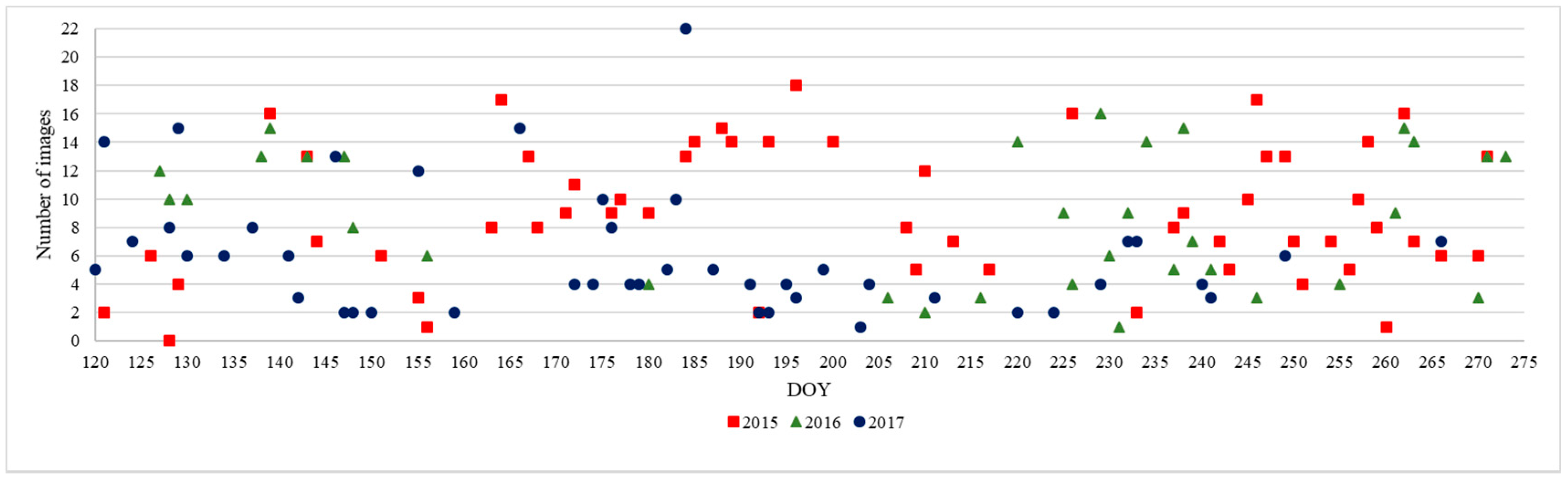
Remotesensing 11 01500 g001
Figure 2. Heilongjiang Province 2015–2017, three-year time series distribution map, including the number of scene images available for each day of the year (DOY).
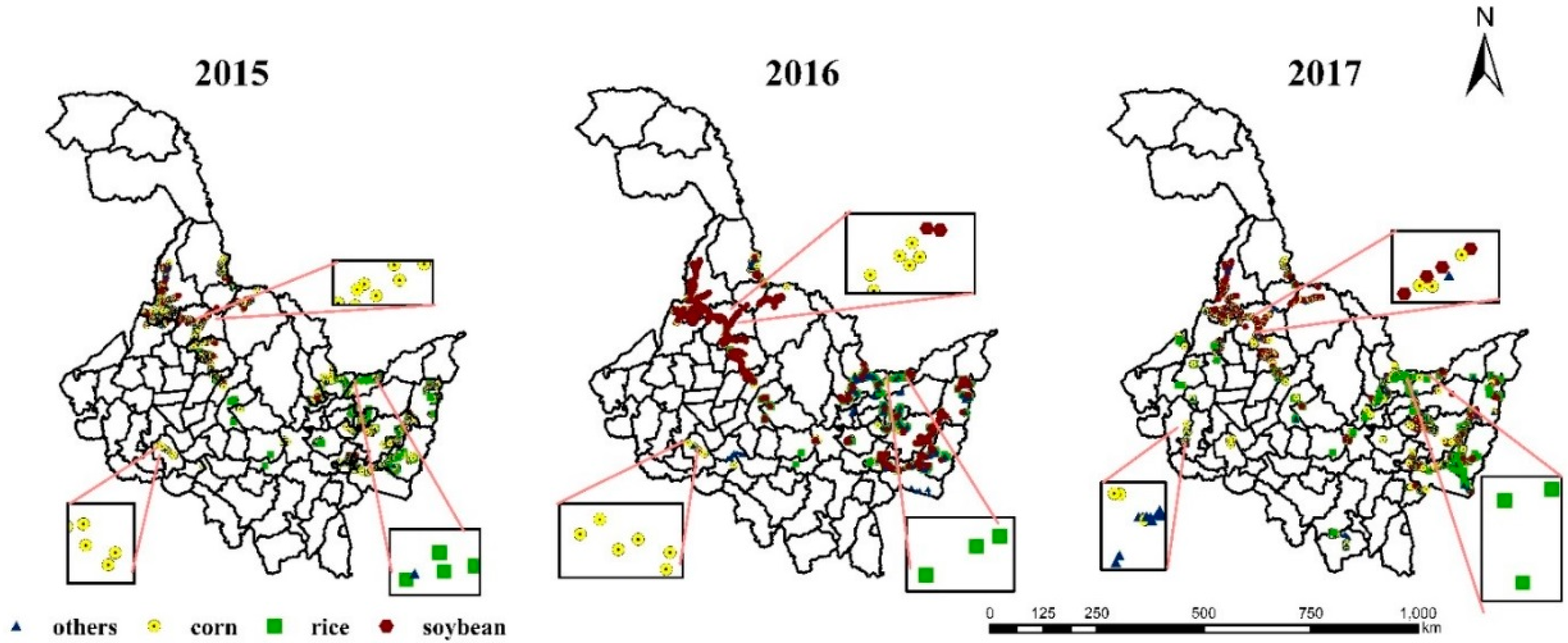
Remotesensing 11 01500 g002
Figure 3. Heilongjiang three-year crop distribution map: yellow for corn, green for rice and red for soybean.
Remotesensing 11 01500 g003
Figure 4. Raster dataset clean and reconstitution multigrid (RDCRMG) coding rules and storage methods.
Remotesensing 11 01500 g004
Figure 5. Heilongjiang Province 2015–2017, three-year time series distribution map, including the number of scene images for each 10 km grid.
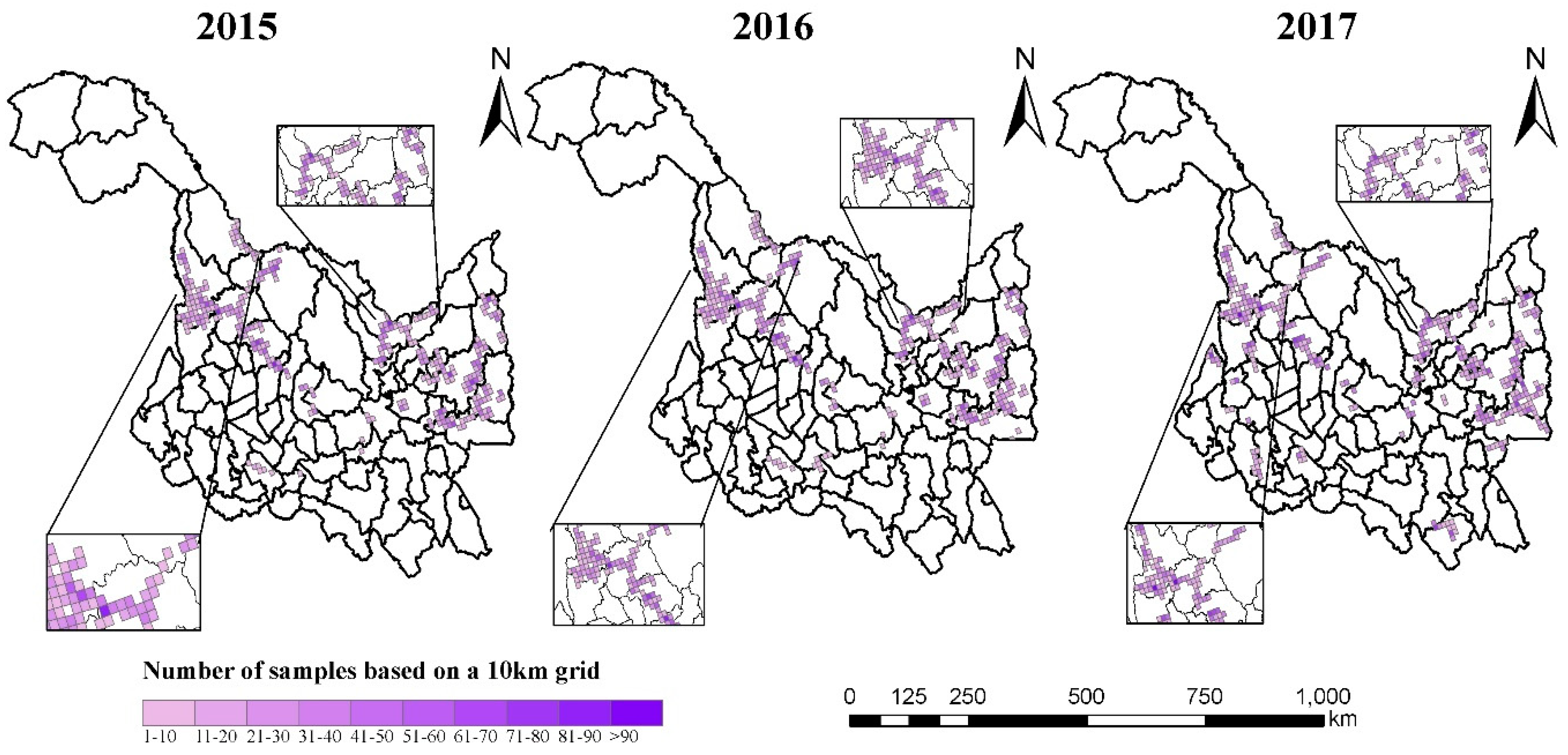
Remotesensing 11 01500 g005
Figure 6. Graph showing how many samples per grid in each year after the three-year sample of Heilongjiang Province was entered into the RDCRMG. Grids from the blank areas do not contain samples. The color depth indicates the number of samples, and each grid has a maximum of 91 samples.
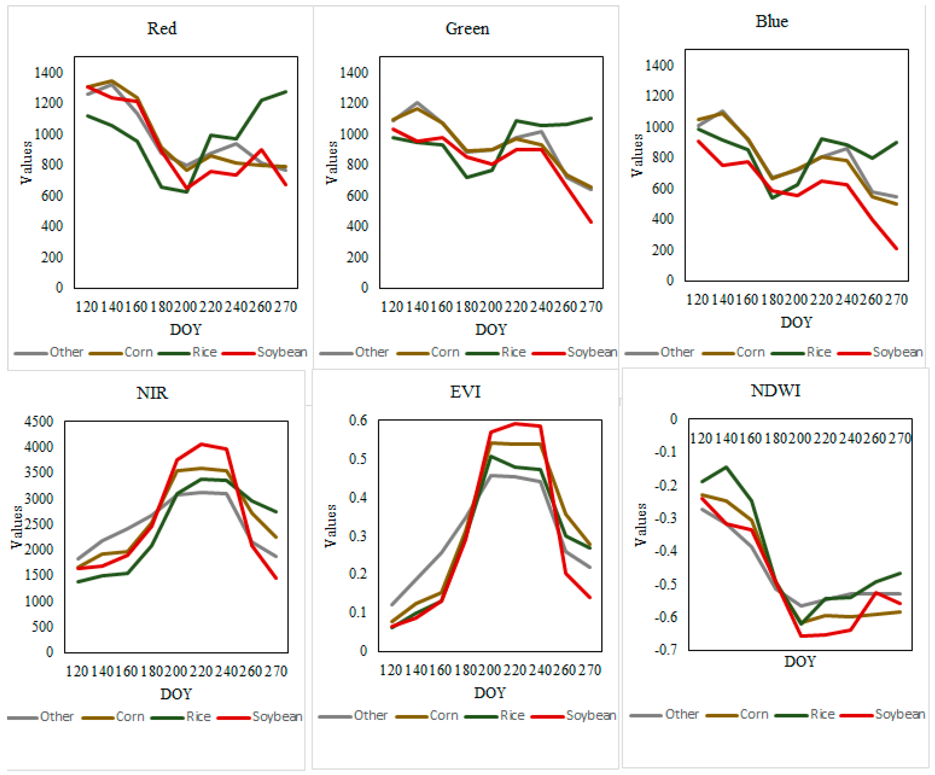
Remotesensing 11 01500 g006
Figure 7. Temporal profile based on the blue, green, red and NIR bands as well as the EVI and NDWI and the timing curves of the corn, rice, and soybean growth periods.
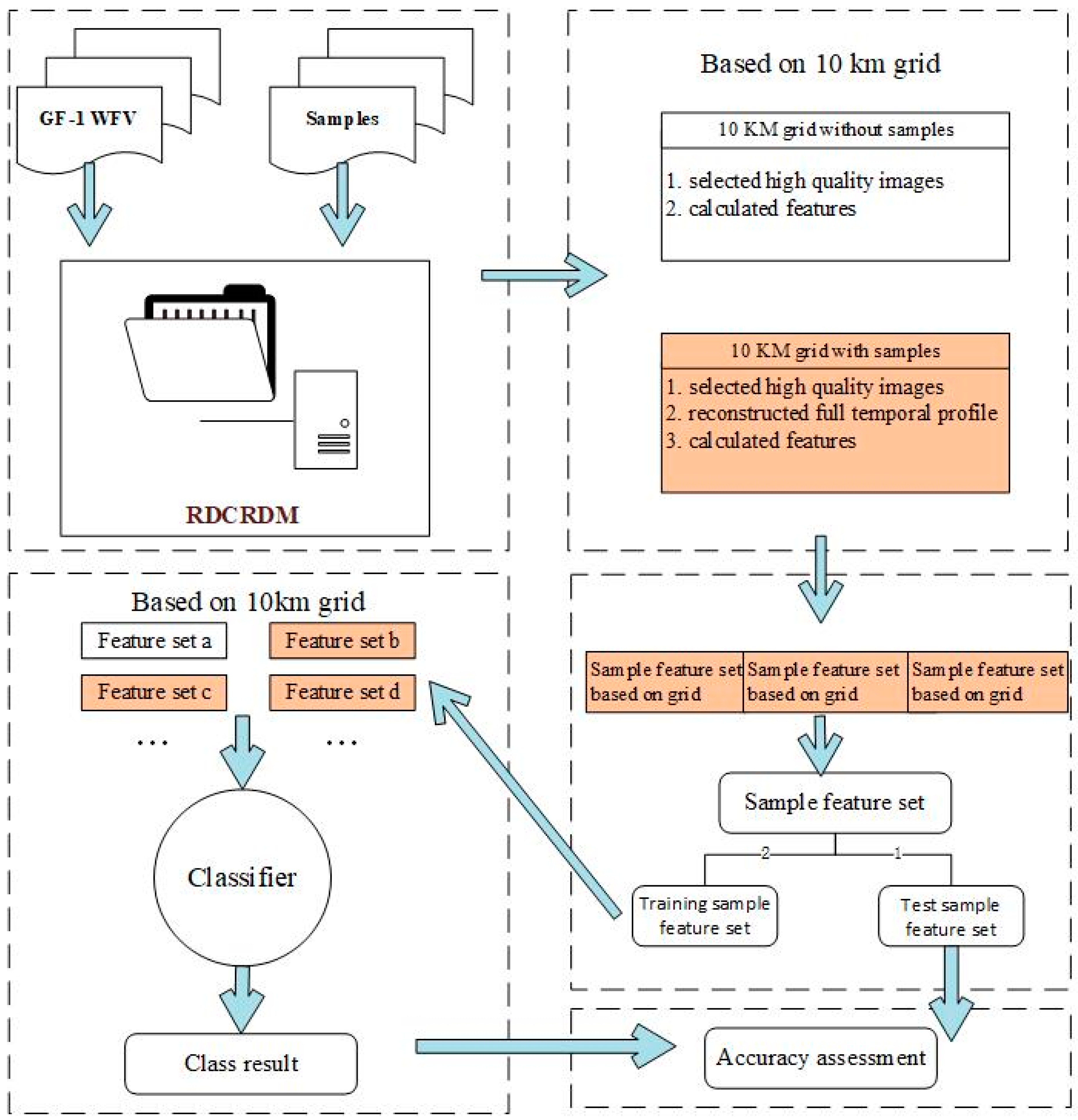
Remotesensing 11 01500 g007
Figure 8. Workflow of our study, including five important steps: (1) data fed into the grid; (2) calculation of multitemporal features; (3) generation of training and test data; (4) classification. Steps 2 and 4 were based on a 10 km grid.
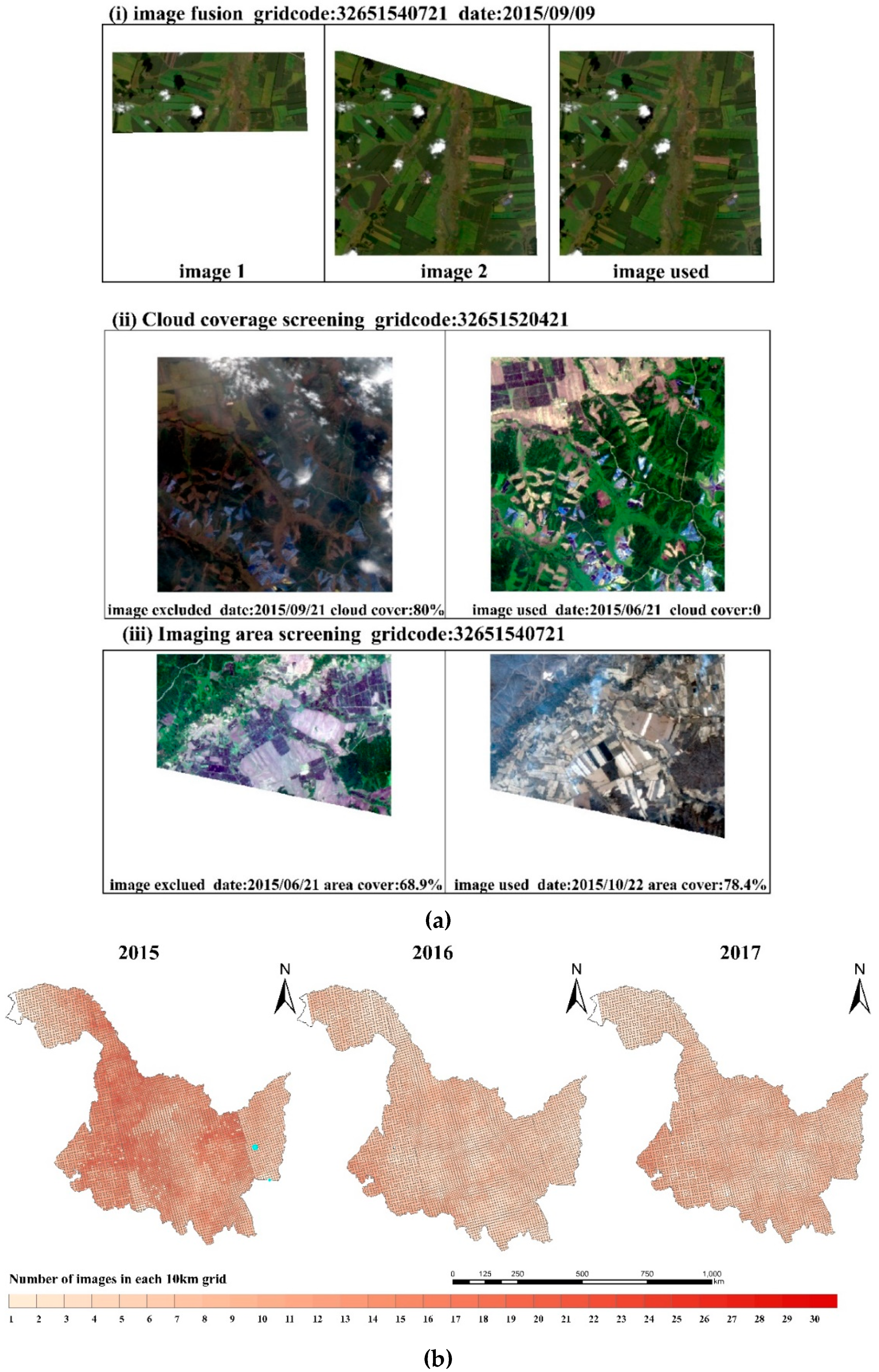
Remotesensing 11 01500 g008
Figure 9. (a) Data selection for three data quality problems. (b) Available dates count statistics of Heilongjiang Province in 2015, 2016 and 2017.
Remotesensing 11 01500 g009
Figure 10. (a) Calculation the union of all observation time points of GF-1 satellite. (b) Full temporal profile reconstruction. (c) Training and classification.
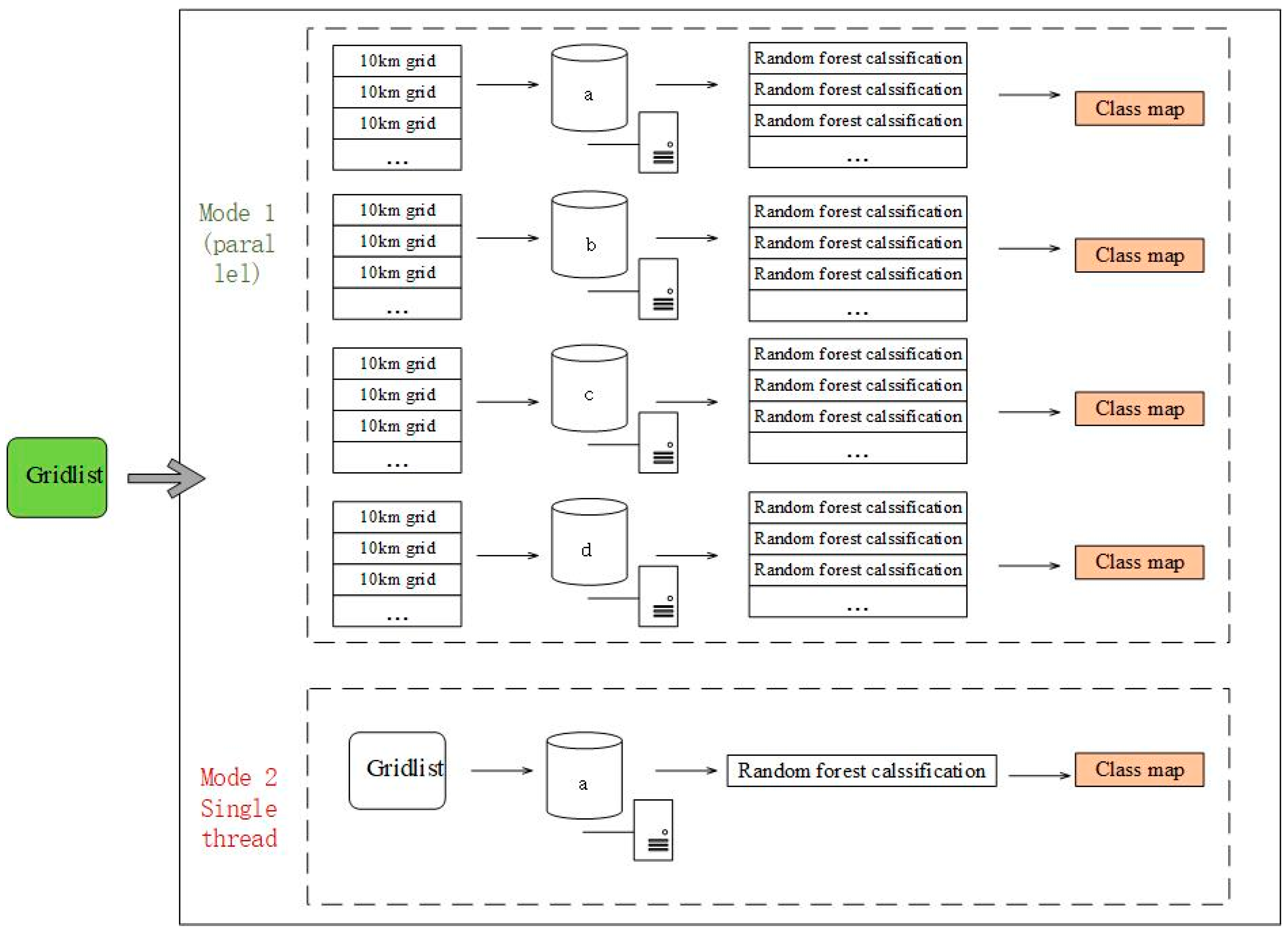
Remotesensing 11 01500 g010
Figure 11. A set of controlled experiments was designed to verify the computational performance improvement of parallel classification with a group of multithread parallel classifications based on computational clusters and a set of single-thread classifications based on one server.
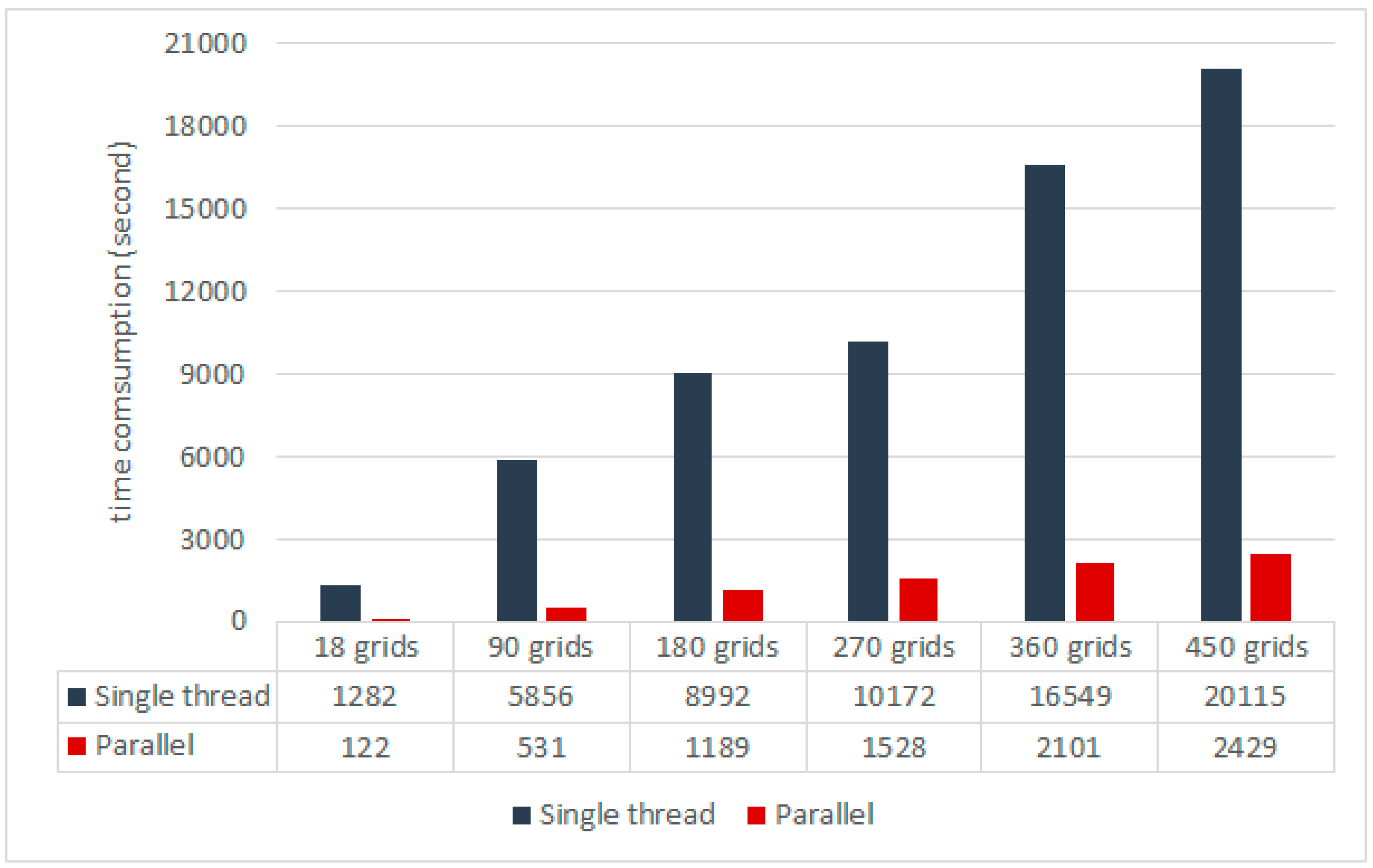
Remotesensing 11 01500 g011
Figure 12. Classification of the time consumption of modes 1 and 2 with different sizes of grids.
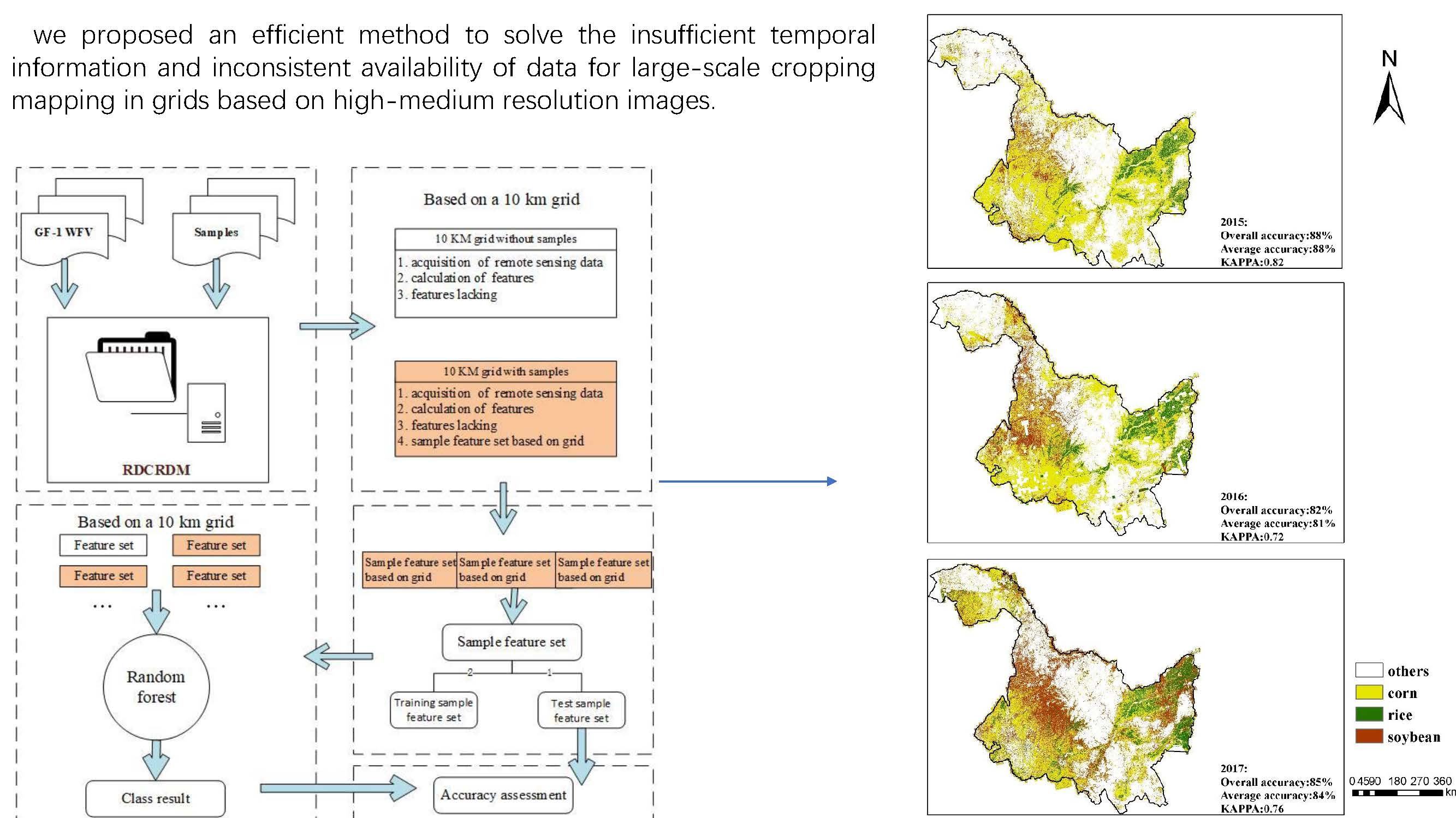
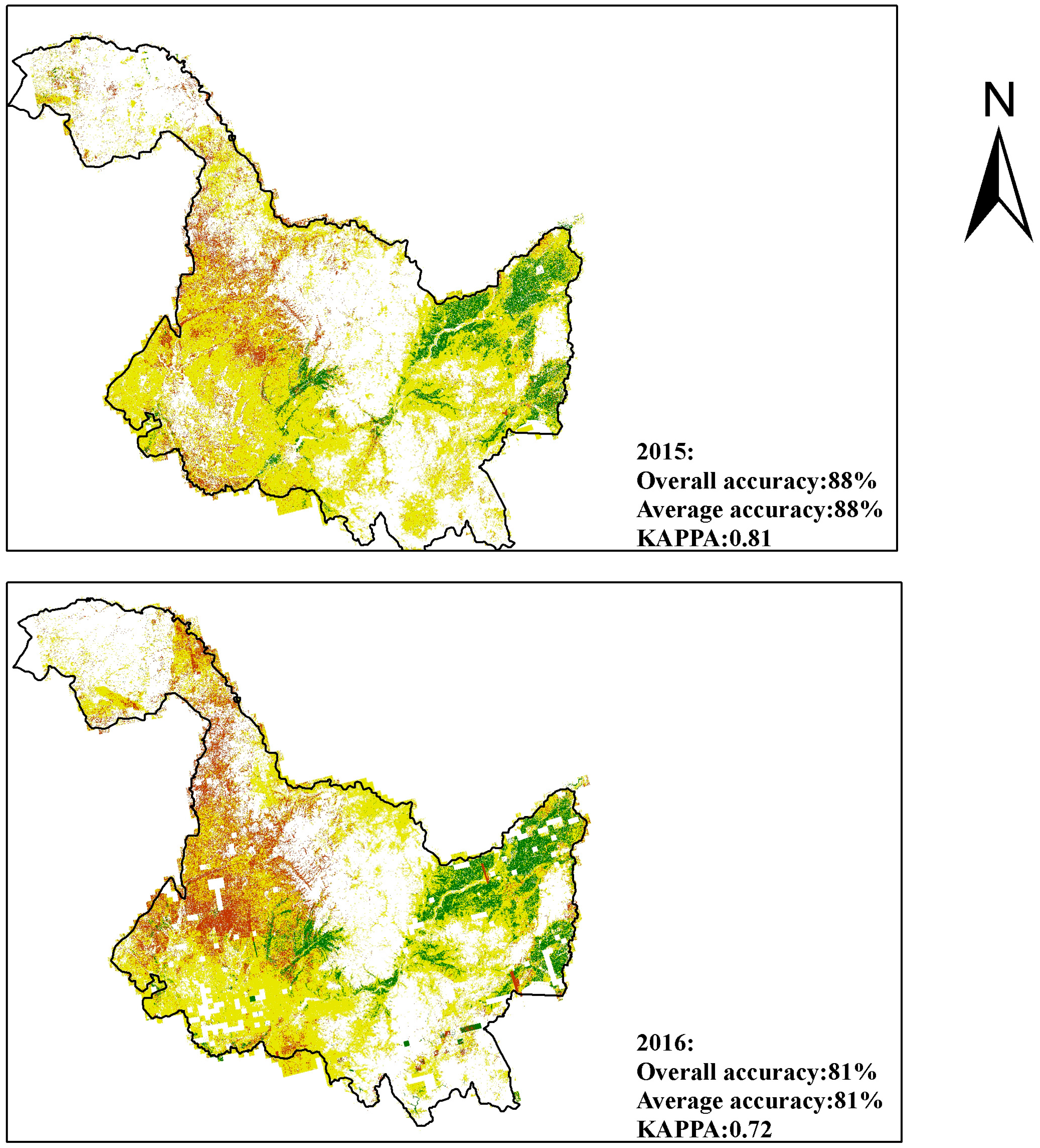
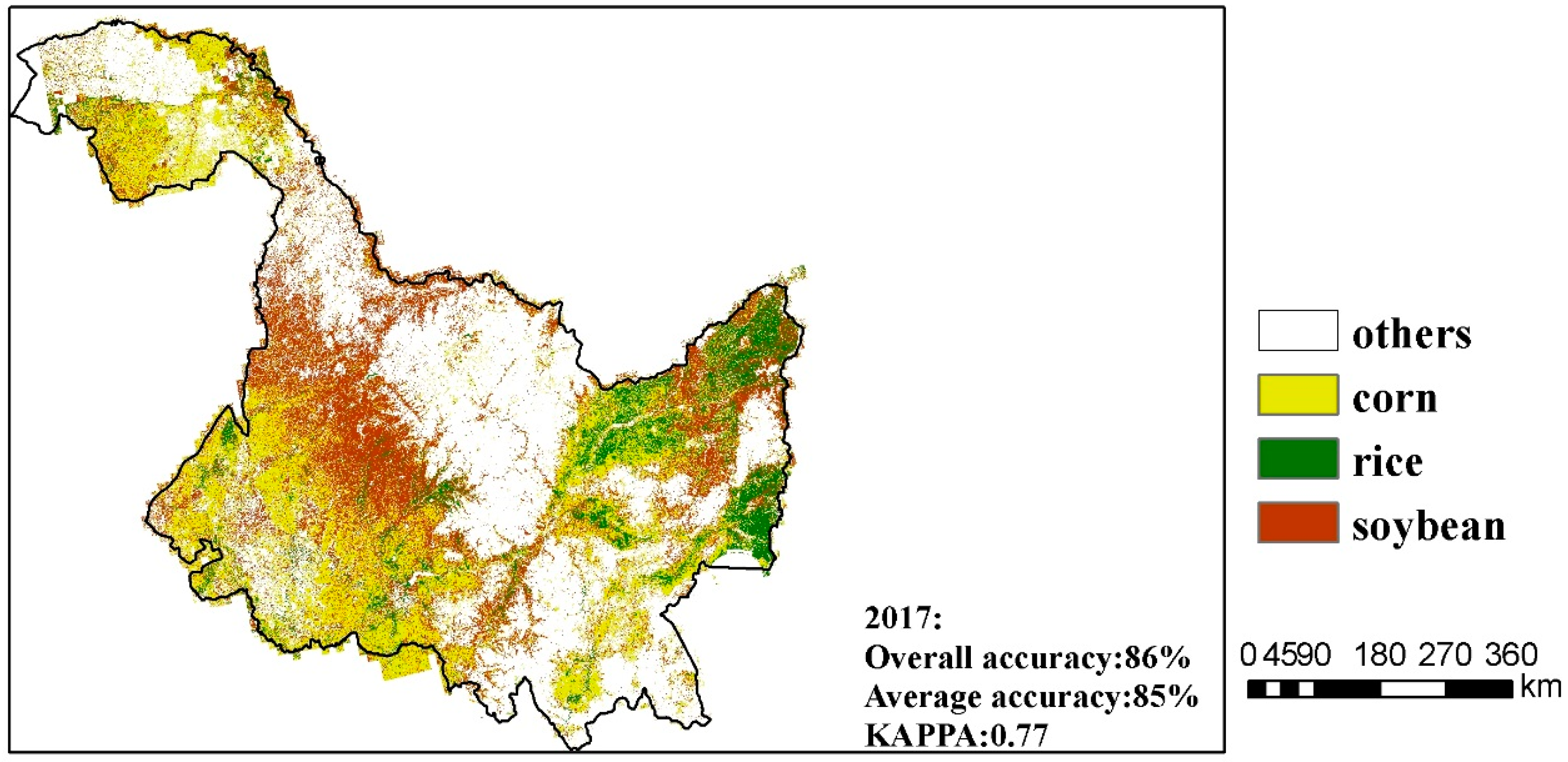
Remotesensing 11 01500 g012
Figure 13. The crop distribution map of Heilongjiang with the overall classification accuracy, average classification accuracy, and Kappa coefficient for year 2015, 2016 and 2017.
Remotesensing 11 01500 g013aRemotesensing 11 01500 g013b
Figure 14. The classification result details of Heilongjiang with four 10 km grids for year 2015, 2016 and 2017.
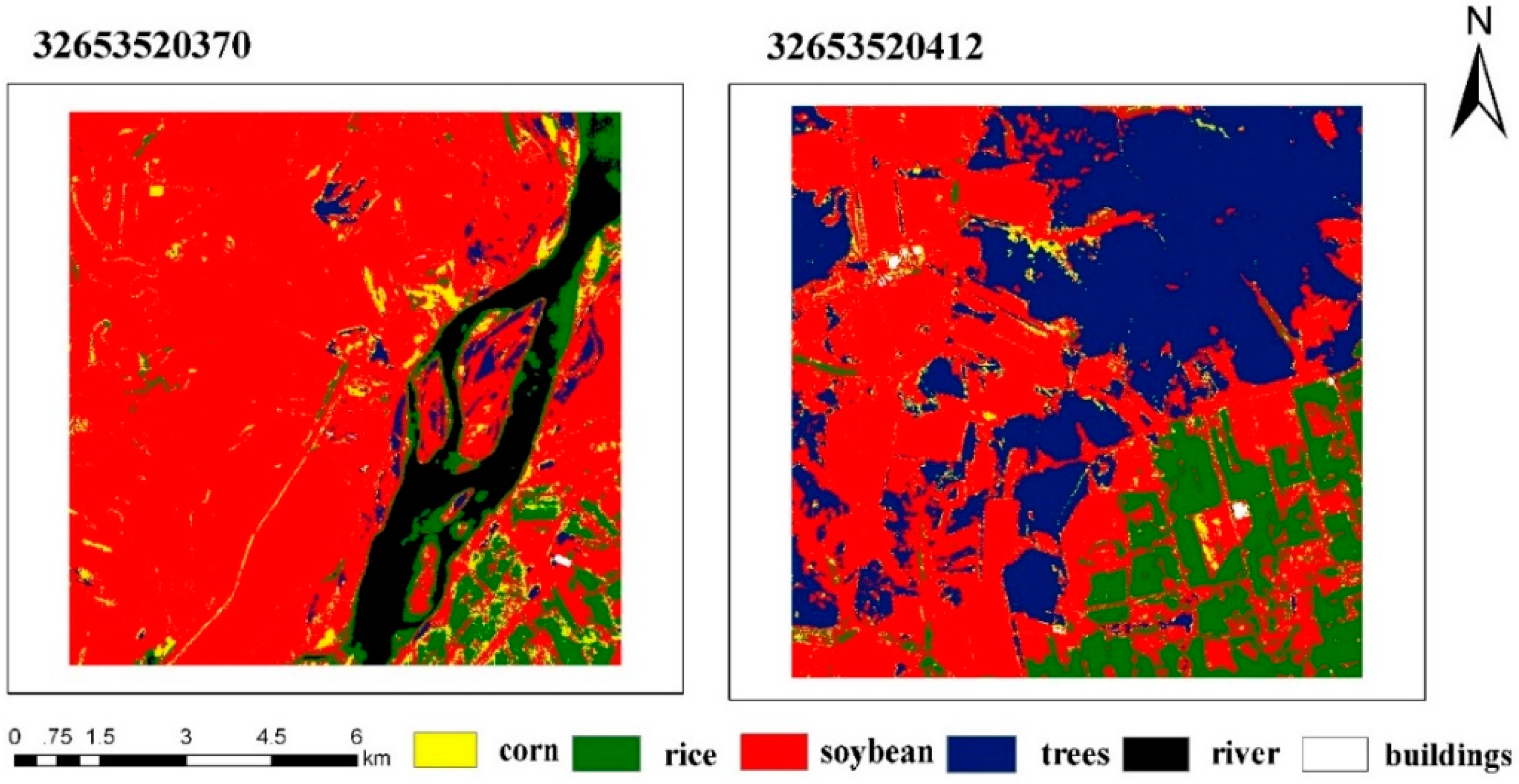
Remotesensing 11 01500 g014
Figure 15. Classification results with trees, rivers, buildings, corn, rice and soybeans.
Remotesensing 11 01500 g015
Table 1. The basic specifications of the computing clusters in terms of the processor and RAM.
Server IDProcessorRAM
Server AIntel E5-2680 × 232 G
Server BIntel E5-2620 × 216 G
Server CIntel E5-2620 × 216 G
Server DIntel E5-2407 × 28 G
Table 2. Parameter group setting details in parameter tuning.
Random Forest AlgorithmSupport Vector Machine
n_estimators 50, 100, 150, 200, 250, 300, 350, 400, 450, 500Kernel Function: linear, C: [1,10,100,100,1000]
max_features ‘auto’, ‘sqrt’, ‘log2’Kernel Function: poly, C: [1], degree: [2,3]
Kernel Function: rbf, C: [1,10,100,100,1000], gamma: [1,0.1,0.01,0.001]
n_estimators: number of decision trees; max_features: number of features of the best segmentation point; C:Cost and slack parameter.
Table 3. Comparison of the accuracy of the classifiers.
ClassifierRandom Forest AlgorithmSupport Vector Machine
Overall accuracy (%)8684
Average accuracy (%)8583
kappa0.760.74
Table 4. Accuracy comparison of the GF- WFV and Sentinel-2 images.
ClassifierGF-1 WFVSentinel-2
Overall accuracy (%)8377
Average accuracy (%)8283
Kappa0.680.70
Number of images107
Table 5. Comparison of the accuracy among the widely used nonparallel classification methods. A refers to the method we propose, and B refers to the widely used classification methods.
Experiment-IExperiment-IISample Count
UA (%)PA (%)UA (%)PA (%)
Corn85958596159
Rice9188769224
Soybean9768977141
Other8269845439
AA:87OA:86AA:86OA:86
AA: Average accuracy; OA: Overall accuracy; UA: User accuracy; PA: Producer accuracy.
Table 6. Confusion matrix of the three-year classification results, the user accuracy and producer accuracy of various crops, the overall classification accuracy, and the average classification accuracy.
Reference Class
Predicted ClassCorn Rice Soybean Other Total UA (%)
2015Corn6999162574593
Rice241842221387
Soybean5113641743684
Other466719625577
Total820200389240164988
PA (%)8592948288
2016Corn6518592774587
Rice151894521389
Soybean910336943677
Other6722715925562
Total824199426200164981
PA (%)7995798081
2017Corn6975311274594
Rice361760121393
Soybean640370243685
Other8551215325560
Total872185 409173164985
PA (%)7995909186
UA: User accuracy; PA: Producer accuracy.
Table 7. Leave one year out method accuracy assessment result.
Year of Classification ResultOverall Accuracy (%)Average Accuracy (%)
20157073
20166467
20177165

