Methods for Earth-Observing Satellite Surface Reflectance Validation


Image Processing Lab, South Dakota State University, Brookings, SD 57007, USA
*
Author to whom correspondence should be addressed.
Remote Sens. 2019, 11(13), 1543; https://0-doi-org.brum.beds.ac.uk/10.3390/rs11131543
Submission received: 22 May 2019
/
Revised: 21 June 2019
/
Accepted: 25 June 2019
/
Published: 28 June 2019
(This article belongs to the Special Issue Cross-Calibration and Interoperability of Remote Sensing Instruments)
Abstract
:In this study an initial validation of the Landsat 8 (L8) Operational Land Imager (OLI) Surface Reflectance (SR) product was performed. The OLI SR product is derived from the L8 Top-of-Atmosphere product via the Landsat Surface Reflectance Code (LaSRC) software and generated by the U.S. Geological Survey (USGS) Earth Resources Observation and Science (EROS) Center. The goal of this study is to develop and evaluate proper validation methodology for the OLI L2 SR product. Validation was performed using near-simultaneous ground truth SR measurements during Landsat 8 overpasses at 13 sites located in the U.S., Brazil, Chile and France. The ground truth measurements consisted of field spectrometer measurements, automated hyperspectral ground measurements operated by the Radiometric Calibration Network (RadCalNet) and derived SR measurements from Airborne Observation Platforms (AOP) operated by the National Ecological Observatory Network (NEON). The 13 sites cover a broad range of 0–0.5 surface reflectance units across the reflective solar spectrum. Results show that the mean reflectance difference between OLI L2 SR products and ground truth measurements for the 13 validation sites and all bands was under 2.5%. The largest uncertainties of 11% and 8% were found in the CA and Blue bands, respectively; whereas, the longer wavelength bands were within 4% or less. Results consistently indicated similarity between the OLI L2 SR product and ground truth data, especially in longer wavelengths over dark and bright targets, while less reliable performance was observed in shorter wavelengths and sparsely vegetated targets.
1. Introduction
Since 1972, users have relied upon Landsat satellite data for historical study of land surface change. However, post-production processing must be performed to analyze land surface change and create application ready data-sets. To alleviate this burden, a “higher-level” Landsat Surface Reflectance (SR) product was developed by the U.S. Geological Survey (USGS) as an initial effort to support land surface change studies. Landsat SR is an essential product desired by users to monitor the land surface reliably and is input for developing higher level surface geophysical parameters to detect overall land cover changes [1].
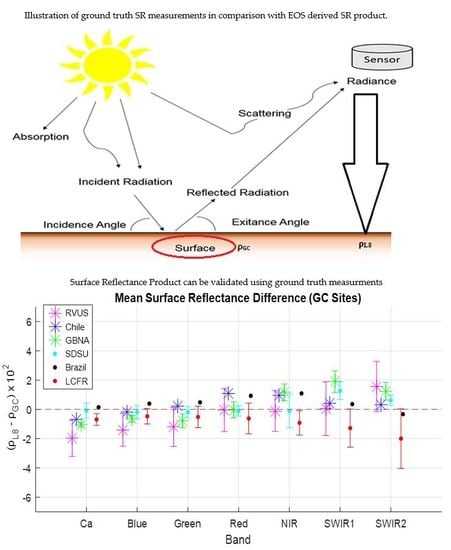
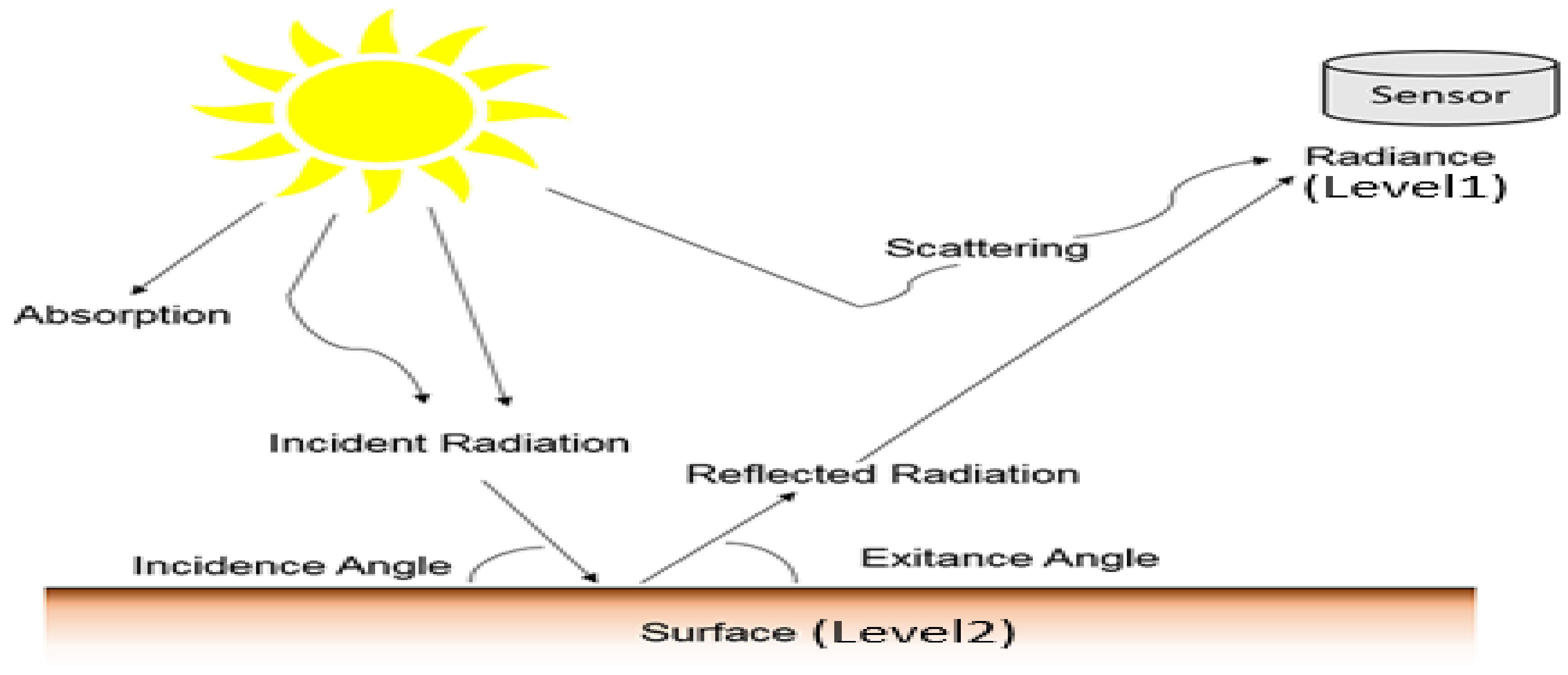
This study focuses on the validation of the Landsat 8 Operational Land Imager (OLI) Level 2 (L2) SR product as generated by USGS and Earth Resources Observation and Science (EROS) Center. SR is derived from satellite Level 1 (L1) top of atmosphere (TOA) reflectance corrected for the temporally, spatially and spectrally varying scattering and absorbing effects of atmospheric gases/aerosols. Generally, the calibration of earth-observing satellites involves the use of the TOA L1 product to monitor the satellite’s radiometric response over time. Whereas, validation provides an accuracy assessment of the SR product (L2) which is derived from the TOA (L1) product. Figure 1 illustrates the difference between the L1 and L2 products.
The L8 OLI L2 SR product spatial, spectral and radiometric characteristics provides the remote sensing community with a vital source of environmental change. For instance, vegetation biophysical characteristics such as leaf area index values, canopy cover and biomass have been extensively retrieved from the use of SR data. Thematic forest classifications can be obtained from SR data to quantify forest productivity and cover density. Additionally, through evaluating land cover of any type, the SR data can be used to detect seasonal dynamics by using temporal Landsat data [3].
Due to the high demand of SR product applications, it is necessary to validate the OLI L2 surface reflectance products to ensure accuracy and precision of the sensor measurements. However, due to the lack of surface measurements at the required spatial and spectral resolution for a given site, the direct validation of OLI L2 products becomes problematic. Thus, developing methods to validate the atmospherically corrected OLI L2 SR product and provide a preliminary validation of the product is the primary focus of this work.
Two potential methods for the validation of OLI L2 product were considered: (i) ground truth acquiring surface reflectance measurements at selected vicarious calibration sites during Landsat 8 overpasses; and (ii) derived surface reflectance measurements acquired from overflights of airborne sensors acquiring low-altitude data during Landsat 8 overpasses. As ground truth measurements are acquired directly at the surface, they require no atmospheric correction. Compared with the airborne derived SR based approach, the ground truth SR based approach is more convenient to operate and the cost is lower. However, the low-altitude airborne sensor data can be acquired over much broader areas than can be directly measured with a portable instrument. For the purposes of this study, both sets of surface measurements will be considered as “ground truth.”
This paper is organized as follows: Section 1 presents a general overview of the L2 product and brief descriptions of the surface measurement datasets. Section 2 discusses the techniques developed for both validation methods. Section 3 discusses the analysis results. Finally, Section 4 offers a general conclusion.
1.1. Landsat 8 Operational Land Imager (OLI) Overview
1.1.1. L8 OLI Information
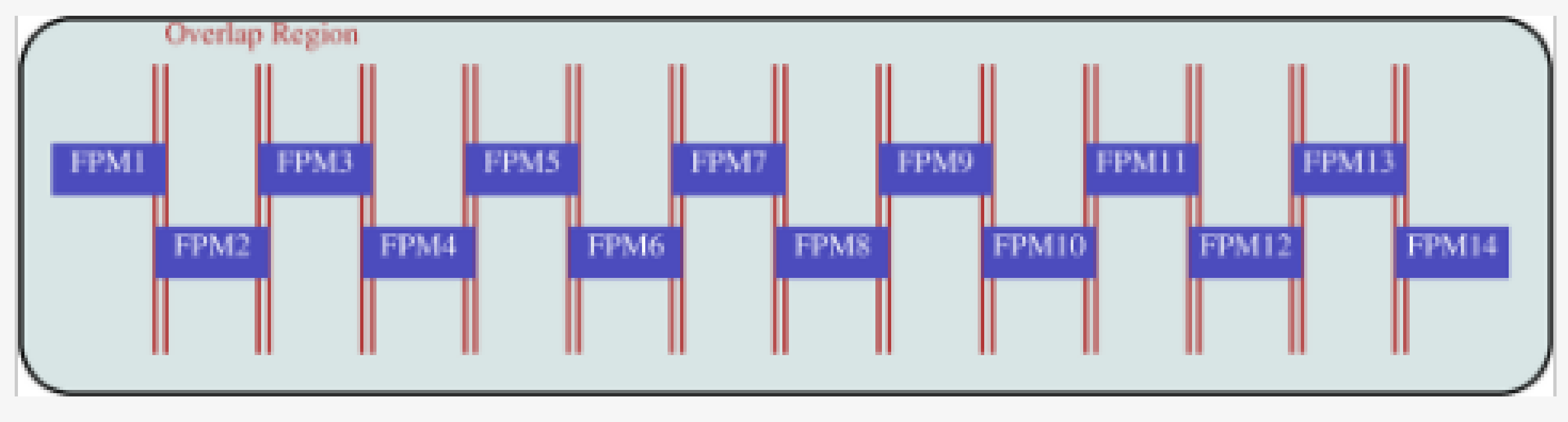
Landsat 8 is the latest platform in the 40-year Landsat series of satellites. The OLI has nine spectral bands with a spatial resolution of 30 m for Bands 1 to 7 and 9. The resolution for Band 8 (panchromatic) is 15 m. Landsat 8 has a temporal resolution of 16 days and its approximate scene size is 170 km north-south by 183 km east-west, with a 185 km swath width. OLI sensor has a pushbroom configuration, 12-bit radiometric resolution, and approximately 7000 detectors in each of the multispectral bands [4,5]. The OLI detectors are separated into 14 Focal Plane Modules (FPMs), each FPM contains 494 detectors per band. The OLI FPMs are shown in Figure 2 below.
1.1.2. Landsat Surface Reflectance Code (LaSRC) Description
The Landsat Surface Reflectance Code (LaSRC) algorithm was developed to derive the OLI L2 SR products through atmospheric correction of the OLI L1 products [6]. LaSRC code is publicly available [7] and has been operationally used by the USGS and NASA to generate Landsat analysis ready data and SR products [8]. LaSRC is based on the 6S radiative transfer code [9], it performs aerosol inversion with an improved determination based on the red to blue band reflectance ratio. Auxiliary climate data are extracted from a spatially explicit climatology of Moderate Resolution Imaging Spectroradiometer (MODIS) and Multi-angle Imaging SpectroRadiometer (MISR) data [10].
1.2. Validation Approaches of OLI L2 Product and Data Product Description
1.2.1. OLI L2 Validation Approach Using Ground Truth Measurements
A total of six ground truth test sites were used in this study to validate the OLI L2 SR product located in Chile, Brazil, Namibia, France, and, the states of Arizona (AZ) and South Dakota (SD). A broad geographic distribution provides two main opportunities for validation: first, the OLI L2 SR product is analyzed and compared over different land cover types, and, second, the OLI L2 SR product validation is considered under different atmospheric conditions. More details on ground truth measurement sites and data processing will follow in Section 2.
OLI Validation via ground truth measurements consisted of two sets of acquired SR measurements: (i) field SR measurements made by a field spectrometer carried over the sites in SD USA, Brazil and Chile [11]; (ii) an automated hyperspectral ground measurement system operated by the Radiometric Calibration Network (RadCalNet) that provides continuous measurements of in-situ surface reflectance and atmosphere measurements in three instrumented sites: Railroad Valley Playa in the US (RVUS), LaCrau in France (LCFR) and Gobabeb in Namibia (GBNA) [12].
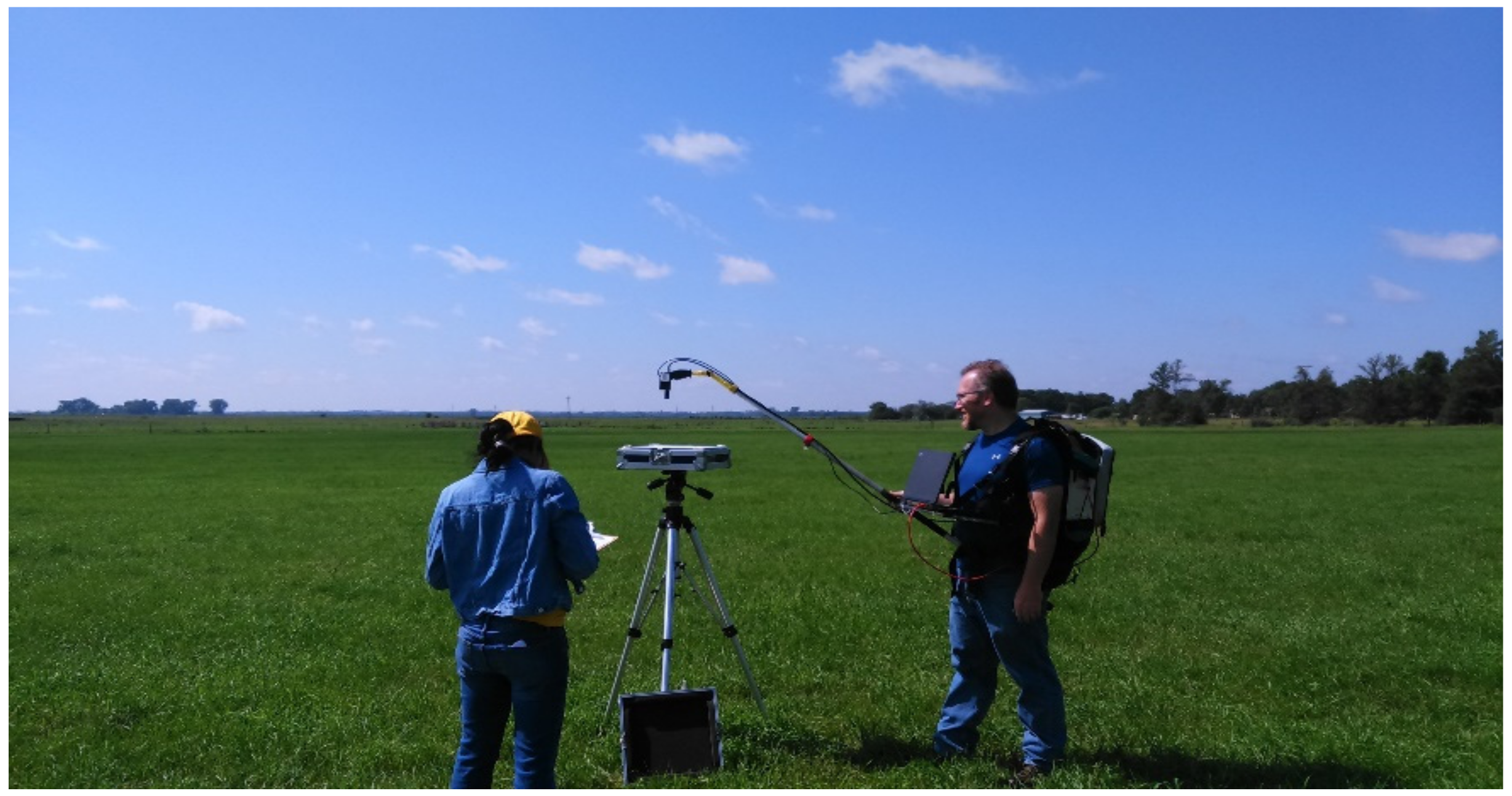
The field SR measurements were measured via a handheld field hyperspectral spectrometer device, designed to cover the solar spectral range. The spectrometer was carried on the field in a predetermined pattern and was equipped with a fiber optic probe to retrieve the spectral signatures of the ground sites use in this study. Shown in Figure 3 is a surface reflectance collection at the South Dakota State University (SDSU) site [13]. The foreoptic is mounted to a boom arm that keeps it away from the user, thereby ensuring that the surface being measured is free of shadows. All SR measurements are made at predetermined points throughout the site collection [14].
The field spectrometer gives a 1.4-nm spectral resolution from 350 to 1000 nm and 10-nm spectral resolution for the 1000–2500-nm spectral range. The spectrometer output is interpolated within the data collection software and the results are sampled at a 1-nm spacing across the entire spectral range. [15,16,17,18,19]. Figure 4 shows the hyperspectral surface reflectance curves of the sites analyzed in this study. The SR measurements are determined by spatially averaging over the test area and band averaging for each of the bands of OLI [13], more details on the sites and data processing will be presented in Section 2.
The second set of ground truth measurements used in this study was based on SR measurements provided by the Radiometric Calibration Network (RadCalNet) [13]. The RadCalNet operates automated ground instrumentation that provides continuous measurement of atmosphere and in-situ SR on cloud-free days. Surface measurements are provided at nadir view every 30 min from 9:00 to 15:00 local time, over a spectral range of 400 nm up to 2500 nm at a 10 nm spectral resolution [20].
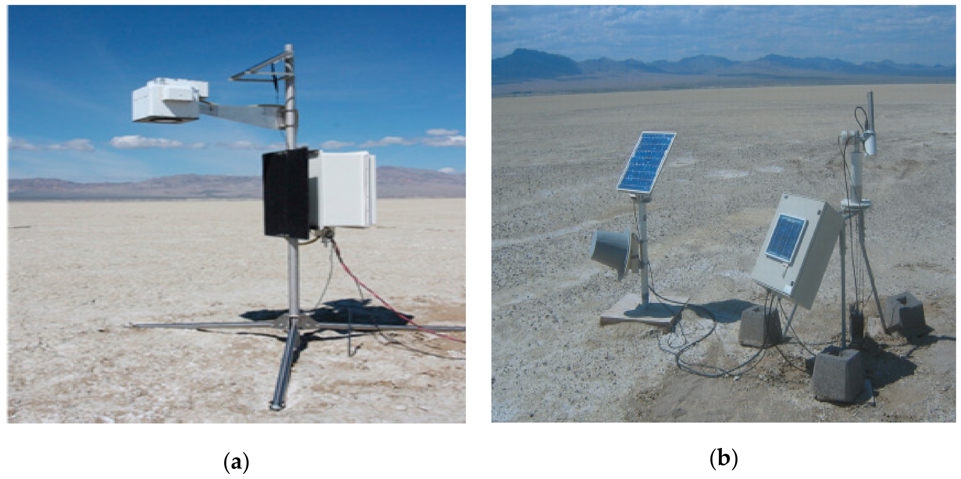
RadCalNet operated instrumentation consist of (i) four ground-viewing radiometers (GVRs) installed to make the in-situ hyperspectral SR measurements [21] (Figure 5a); (ii) Cimel sun photometer (part of the Aerosol Robotic Network) used to make atmospheric measurements (Figure 5b) such as the aerosol optical depth, the Angstrom exponent and water vapor [22,23].
The RadCalNet GVR is a multispectral eight-channel radiometer that covers the visible to the SWIR bands [24]. Data obtained from the GVR must be converted to hyperspectral and spatially averaged SR results similar to those obtained via a field spectrometer device. Therefore, the SR of each GVR multispectral channel is calculated using Equation (1):
where is the multispectral SR for a given band (W m−2 sr−1 μm−1)·V−1, C is the GVR calibration coefficient V is the GVR output voltage (V), d is the earth-sun-distance normalized to the average, is the solar zenith angle, is the solar beam atmospheric transmission (unitless), is the spectral solar exoatmospheric irradiance (W m−2·μm−1), is the diffuse spectral sky irradiance (W m−2·μm−1). The variables and are determined using MODTRAN, whereas, the calibration coefficient C is determined using the solar-radiation-based calibration technique (SRBC) [25].
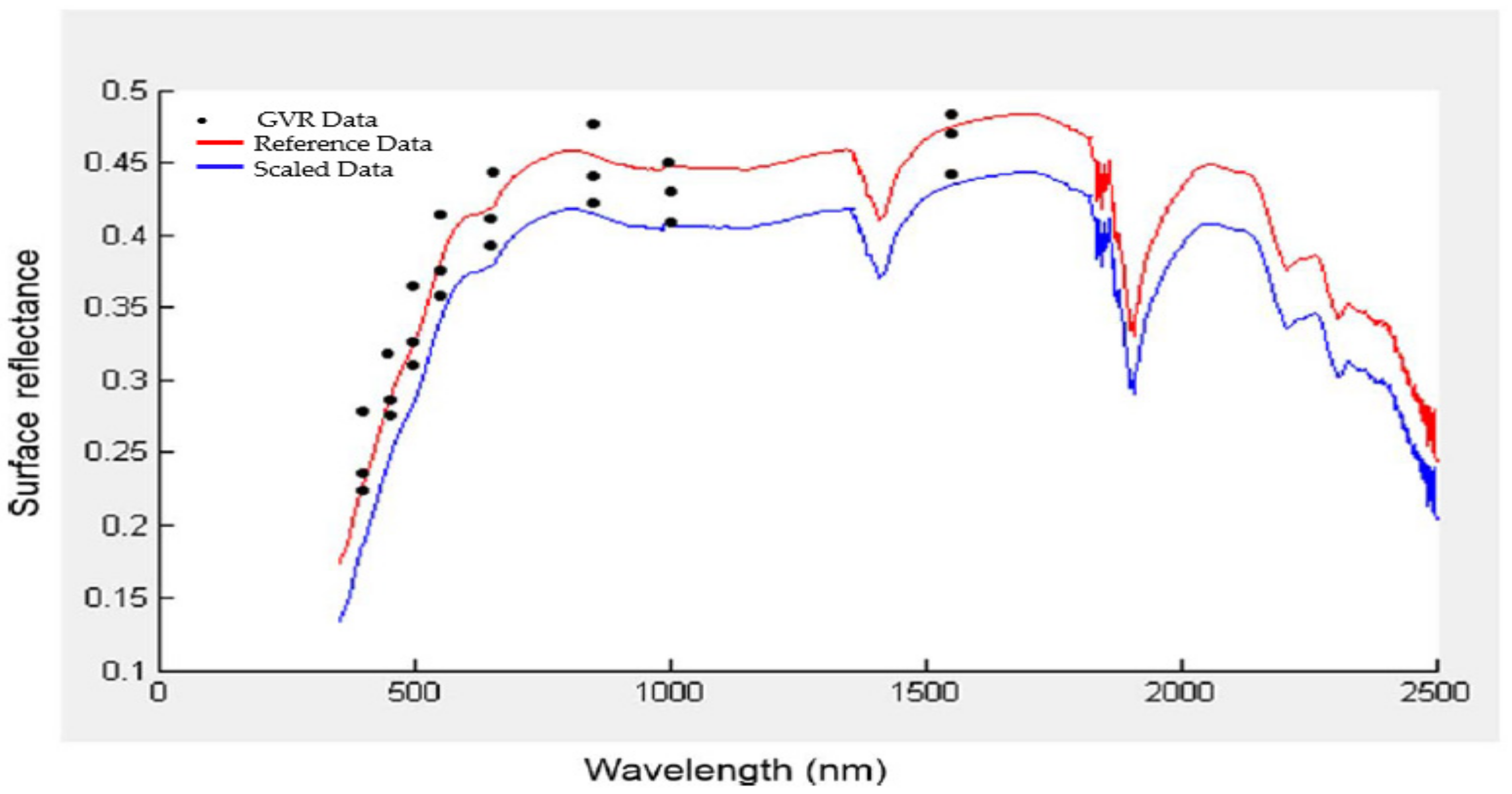
The calculated multispectral SR GVR data (from Equation (1)) is then converted to hyperspectral SR by rescaling a hyperspectral “reference” spectra at the time of the Landsat-8 overpass. This reference hyperspectral spectra was selected from a reference library created from 12 years of in situ measurements that corresponds to the RadCalNet Railroad Valley site. An illustration of how multispectral GVR SR data are used to scale reference hyperspectral SR data is shown in Figure 6 [26,27,28].
1.2.2. OLI L2 Validation Approach Using Airborne Observation Platforms (AOPs)
While ground truth measurements remain the most direct validation approach, the associated footprint is usually very limited. The goal of this section is to provide an alternative method to validate the performance of the OLI L2 SR product by looking at derived SR from Airborne Observation Platforms (AOP) operated by the National Ecological Observatory Network (NEON). NEON SR products are, in turn, considered as independent truth for the purposes of this study. Scale effects between the Landsat and NEON AOP will be discussed in more detail in Section 2.
On-board the NEON AOPs is an imaging spectrometer, which provides potential for high precision observations [29]. The AOP has an approximate altitude of 1000 m, therefore, the radiance received by the NEON Imaging Spectrometer (NIS) is subject to atmospheric effects such as scattering and absorption caused by gases and aerosols. Hence, it is necessary to convert the measured NIS spectral radiance to surface reflectance and remove atmospheric effects. The NEON derived SR product is a calibrated and atmospherically corrected product distributed as scaled reflectance. Therefore, the NIS derived SR reflectance product can be used as ground truth to validate the OLI L2 SR products [30].
NEON flights are conducted annually over strategically located sites across the U.S. within 20 eco-climatic domains [31]. Allowing OLI L2 SR product validation over numerous domains that represent regions of distinct landforms, vegetation, climate and ecosystem dynamics [32]. Figure 7 shows a map of the NEON domains that were analyzed in this study (highlighted in red), the sites will be explained in more detail in Section 2.
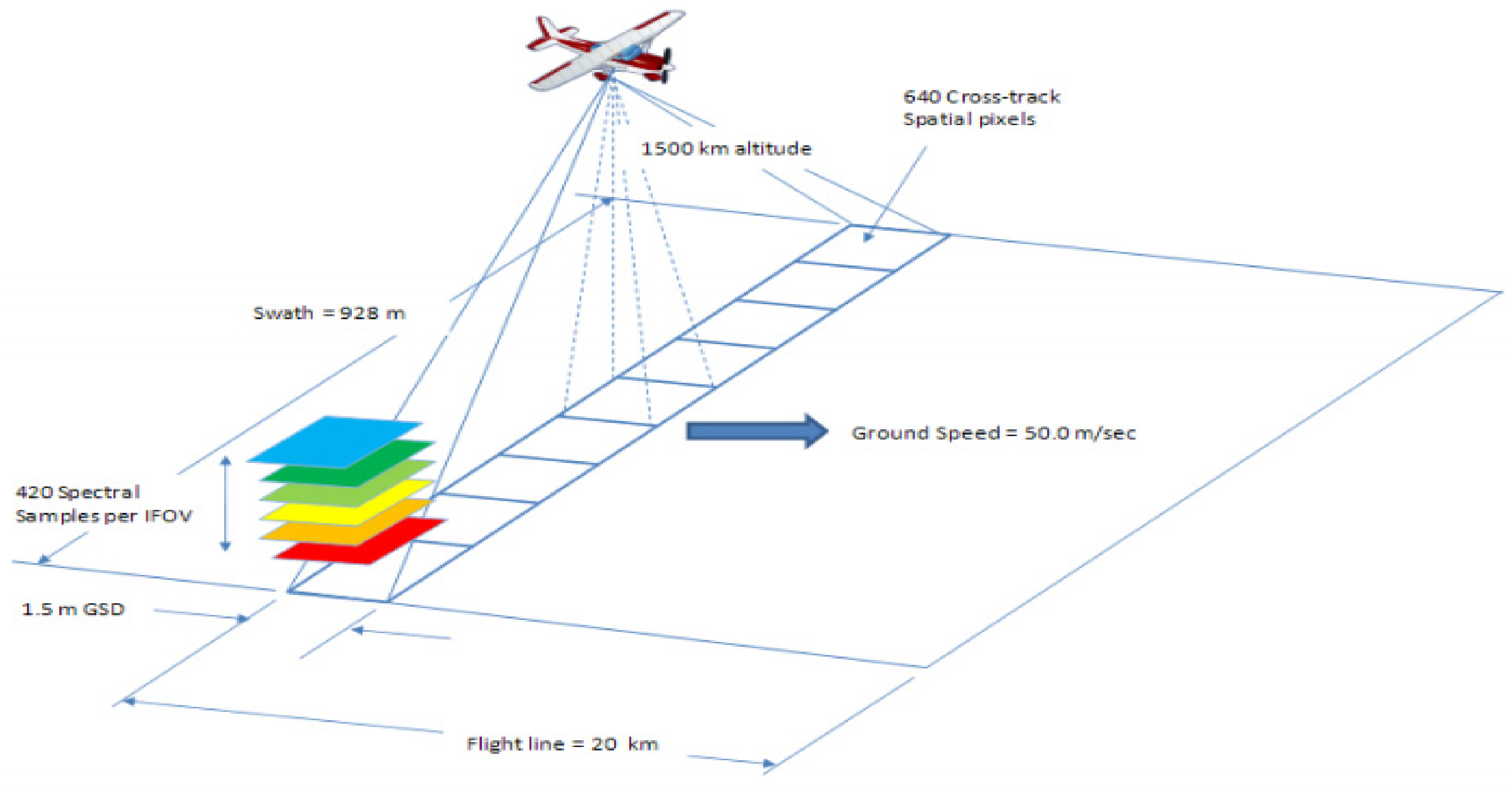
The pushbroom NIS measures upwelling radiance over 426 spectral bands in the solar region between 380 and 2500 nm with a spectral sampling of 0.5 nm. The NIS cross track swath is ~928 m, with an instantaneous field of view (IFOV) of 1.0 mrad, at an altitude above ground level of ~1000 m and covers an area of 5–20 km × 0.600 km × number of flightlines. The ground sampling distance (GSD) is 1 m [33]. The NIS concept is illustrated in Figure 8, and the main differences between the NIS and OLI sensors are listed in Table 1 [34,35].
2. Materials and Methods
2.1. L8 Validation Using Ground Truth Measurements
2.1.1. ROI and Site Selection
This work was conducted at field sites that that are characterized by several criteria, such as high probability of clear skies, high spatial homogeneity, weak directional effects and low probability of atmospheric variability [18,36,37,38,39]. In this study, six test sites were used for direct comparison between OLI and ground truth data. Three of those sites consisted of measurements conducted at RadCalNet sites, the remaining sites consisted of ground campaign measurements [16]. Ground truth SR measurements were measured simultaneously with the L8 OLI overpass over homogeneous plots of vegetation and bright cover types. Table 2 provides additional information for all six ground truth sites.
This study validated the atmospherically corrected OLI L2 SR product, the L2 product scenes, of the sites in Table 2, were obtained from the USGS Earth Explorer on-demand processing system web portal using the 2013 version of the LaSRC code [9]. The number of OLI scenes were based on the L8 coincident overpasses that were listed in Table 3 above. The USGS system generates the full suite of LaSRC based parameters, including TOA reflectance, AOT, SR, and pixel-level quality flags [40,41].
Hyperspectral SR data for the SDSU, Bahia, and Atacama sites were extracted from ASCII text files retrieved from the SDSU Image Processing Laboratory archive. Hyperspectral SR data for the RVUS, LCFR, and GBNA sites were obtained from the RadCalNet portal [12].
2.1.2. Data Processing
Data procedure for both time and location was performed to match-up the ground truth data with the OLI data in order to validate the OLI SR product. The ground measurements were taken during OLI overpasses, therefore, uncertainties caused by changing atmospheric conditions were minimized. The following procedure was used to process the OLI L2 product data:
- Identify the set of OLI overpass dates when ground measurements were simultaneously acquired.
- Perform cloud/shadow/artifact screening in each OLI image using the associated Quality Assurance (QA) band information. This information consists of integer values where each bit represents a quality condition. Visual inspection of the images was also performed to verify the QA band assessment; ROI pixels visually showing clouds/shadows were excluded from further analysis.
- Convert the artifact-free ROI DNs of the OLI images into units of reflectance using scaling factors given in the associated OLI product metadata:where; corresponds to OLI L2 SR product corresponding to band i; is the digital number (pixel value) of OLI L2 product corresponding to band i; SF is the multiplicative scale-factor used to convert DN to SR at band i.
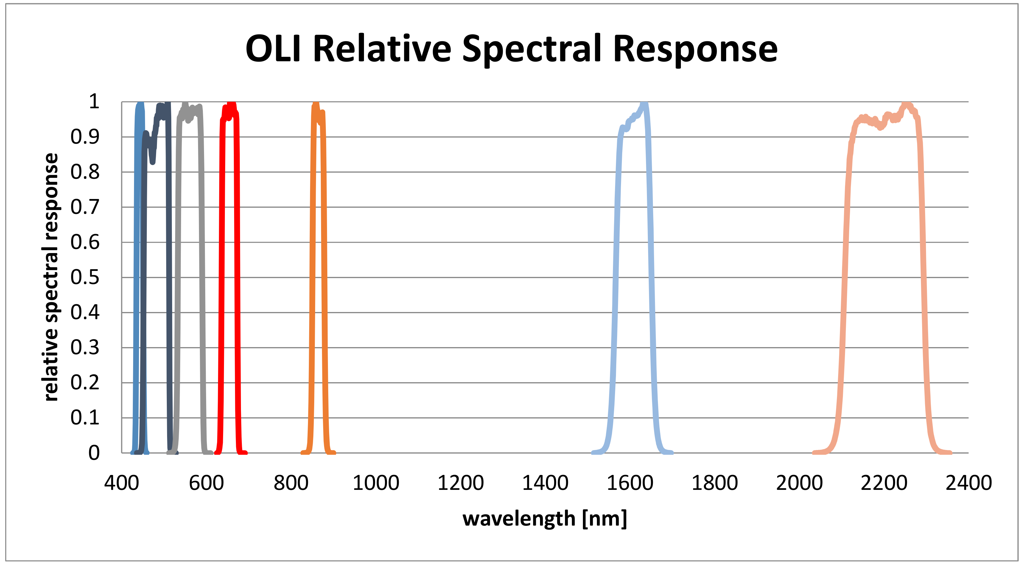
- Ground truth measurements are hyperspectral in nature (as alluded to earlier in Section 1.2), therefore, ground truth reflectance must be converted to match OLI reflective multispectral bands as indicated by the OLI prelaunch Relative Spectral Response (RSR) curves for the CA-SWIR2 bands, as shown in Figure 9 [42]. The multispectral reflectance of the ground truth measurements can be calculated by convolving the continuous ground truth reflectance with the OLI RSR function of the corresponding OLI bands:where, is the multispectral ground truth SR corresponding to band i; is the OLI spectral response function of the corresponding bands; is the hyperspectral ground truth reflectance; and , are the lower and upper wavelength of the spectral range in band i.
- RCN data is generated at a 30-min temporal interval. Therefore, temporal linear interpolation to the RadCalNet data was applied to estimate the measurement(s) during the OLI overpass time.
2.1.3. Analysis
After processing the ground truth and OLI L2 SR data as described in Section 2.1.2 on all six ground truth sites and overpasses from Table 3, statistical analyses were performed to assess the accuracy of the OLI L2 SR () using ground truth SR measurements (). The analysis procedure is described as follows:
First, the accuracy of the L2 product for each band was estimated as follows:
- Generate scatterplots of the OLI L2 SR (vertical axis) vs. the corresponding ground truth SR measurements (horizontal axis) for all of the overpass dates at a given site.
- Perform a linear regression on the scatterplot data and quantify the goodness-of-fit as (i) the estimated R2 of the fit; and (ii) slope and intercept of the regression line; a regression slope of one and intercept of 0 represents ideal agreement between the measurement datasets.
Second, the mean reflectance difference between the OLI L2 SR and ground truth measurements was calculated for the ROI at each of the sites listed in Table 3, on all overpass dates. The mean reflectance difference was used to describe the bias of OLI L2 product (negative, if OLI SR is underestimated and positive, if OLI SR is overestimated).
where, is the mean reflectance difference of OLI L2 SR and ground truth measurements; is the number of ROI pixels for each band λ. is the reflectance difference between the ground truth measurement and OLI L2 reflectance in band λ and pixel i:
where, and are the estimated ground truth and OLI surface reflectance, respectively. Absolute measurements were taken to identify possible bias between the ground truth and OLI measurements.
Similarly, the standard deviation () of the mean reflectance difference () was defined as:
Finally, the root-mean-square error (RMSE), represents the actual statistical deviation of OLI L2 SR from the truth estimate, including the mean bias, and is computed as:
The RMSE value was expressed as a relative percentage of the mean OLI L2 SR to characterize the uncertainty of the OLI L2 SR product. Such analysis was applied to estimate the expected uncertainty of the OLI L2 SR product [40]. Similar approaches were undertaken in the past to characterize Landsat products [42], VIIRS [44] and MODIS SR product [45].
2.2. L8 Validation Using NEON as Ground Truth
2.2.1. ROI and Site Selection
To validate the OLI SR product with the NIS, six sites across the US were selected since the OLI and NIS were imaged simultaneously (to within ±10 min). Near-simultaneous scene pairs were selected in order to minimize potential uncertainties due to atmospheric and solar geometry effects between the OLI and NIS overpass times. Overall, seven scenes were processedand were mainly composed of mixed vegetation. Table 3 shows the metadata for the scenes used.
OLI and NIS overpasses at Santa Rita Experimental Range (SRER) had the largest time difference with 20 min; the scene was used because it is the nearest available time on that date and location. The ROIs were chosen from regions identified as cloud-free and homogeneous, based on available product quality information and visual inspection. The “pixel_qa” band of OLI L2 product was used to identify cloudy regions.
The NIS SR data for all the reported sites in Table 3 were obtained from the NEON data portal [46]. The derived NEON SR is a UTM projection hyperspectral raster product. It is distributed in an open HDF5 format including all 426 bands obtained from the on-board NIS. The HDF5 file includes the derived SR reflectance data, QA and ancillary rasters used as inputs for atmospheric correction, all metadata and ancillary data for every flight line.
2.2.2. Data Processing
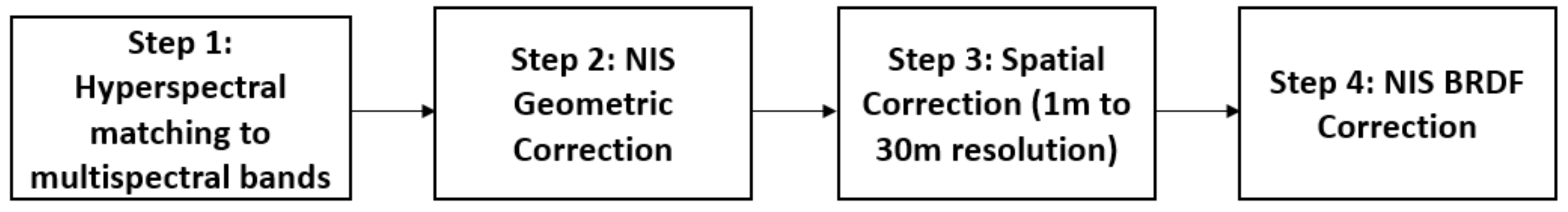
Prior to validating the OLI SR with NIS SR, several necessary corrections to the NIS SR data were made to account for scale differences. Figure 10 outlines the processing flow used to validate OLI SR products with respect to NEON.
As described in Section 2.1.2, spectral conversion of the NIS data to match the OLI spectral response was performed prior to the analysis.
Geometrically Align the OLI and NIS Images
Remote sensing image data potentially contains some degree of geometric distortion due to changes in sensor orientation, effects due to the earth’s rotation about its axis, and terrain effects due to mountains/hills (geometry effects) The OLI is reported to have a 12 m geometric uncertainty [47], while NIS is reported to have a 0.2 m geometric uncertainty [33]. To ensure accurate validation between the OLI and NIS, image registration was applied to the NIS scenes, using the OLI scenes as a reference.
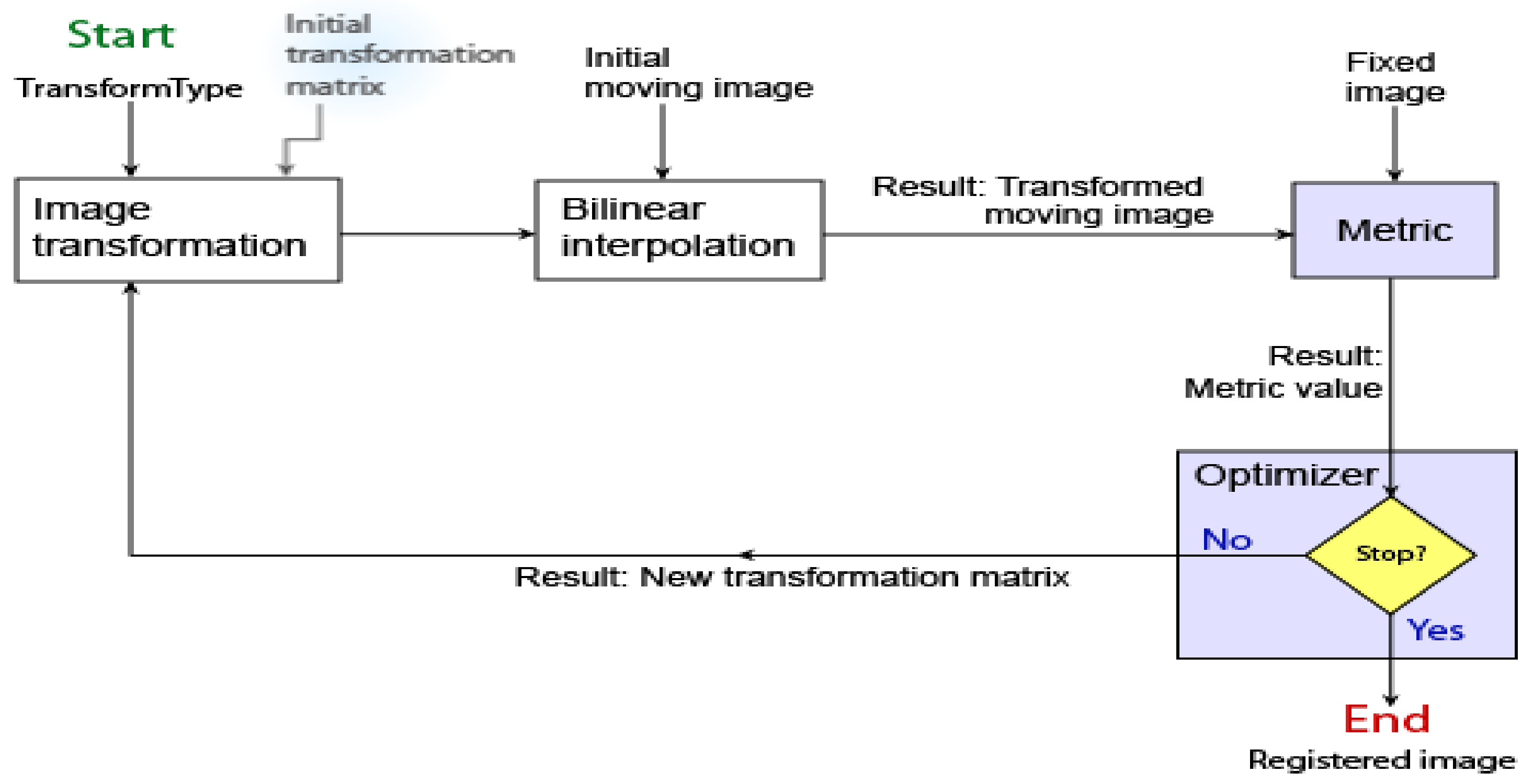
For the purposes of this work, an intensity-based registration approach was performed as there was no set of quality ground control points available. Intensity-based image registration is an iterative process based on a scalar metric representing the degree of similarity between the “moving” NIS image to be registered and the reference “fixed” OLI image [48,49]. Figure 11 shows a basic flowchart of the steps implementing the algorithm.
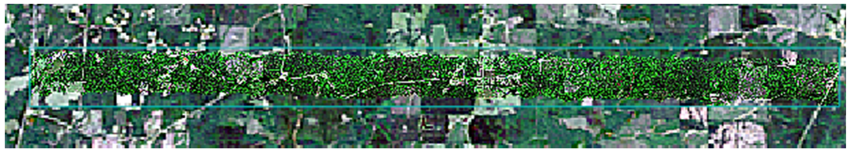
The process starts with a user selected image transformation and an internally determined transformation matrix based on a ‘similarity’ model. For the purposes of this work, a subset of the affine transformation called the similarity transformation was used [50]. The translation, rotation, and scaling of the affine transformation belongs to the similarity transformation. However, a similarity transformation changes all distances within an image with the same ratio, i.e., a similarity transformation preserves shape [51]. The selected similarity transformation and the internally determined matrix determines the specific image transformation that is applied to the NIS image via bilinear interpolation. The image transformation type is a 2-D transformation that aligns the NIS image with the reference OLI image [44]. Next, the ‘Metric’ and ‘Optimizer’ blocks analyze the new NIS transformed image and adjusts the initial transformation matrix to begin the next iteration. The similarity of OLI and NEON images are indicated using the mean square error [52]. The algorithm reiterates itself until it finds a matrix transformation that yields the best possible NIS registration results. In this case, the transformation process stops when the mean square error reaches a point of diminishing returns, at a value of 0.0022 or less [53,54]. An overlaid multispectral registered NIS image with OLI is shown in Figure 12, for clarity purposes a band composite RGB display was used.
In Figure 12, the registration results between OLI and NIS RGB composed images are both very good and are difficult to tell apart visually. The process was repeated for each NEON site in this study.
Resample NIS Product to Correct Spatial Resolution Differences
After performing the geometric registration on the multispectral and geometrically corrected NIS scenes, the image data from both sensors were georeferenced to the WGS 84 coordinate system. However, a residual spatial resolution mismatch remains. The OLI SR product has a spatial resolution of 30 × 30 m, whereas the NIS product has a 1 × 1 m spatial resolution. The NIS SR images were resampled to match the OLI SR image spatial resolution. The resampling process was performed using the map coordinates of every scene to locate the OLI pixels. A binary mask was then created for every OLI pixel and applied to the corresponding NIS pixels. The mean of the NIS pixels within the binary mask was taken to represent one OLI pixel at 30 × 30 m resolution, thus leaving us with a NIS SR that is multispectral, geometrically and spatially corrected.
Correct BRDF Effects in Resampled NIS Product with Respect to OLI
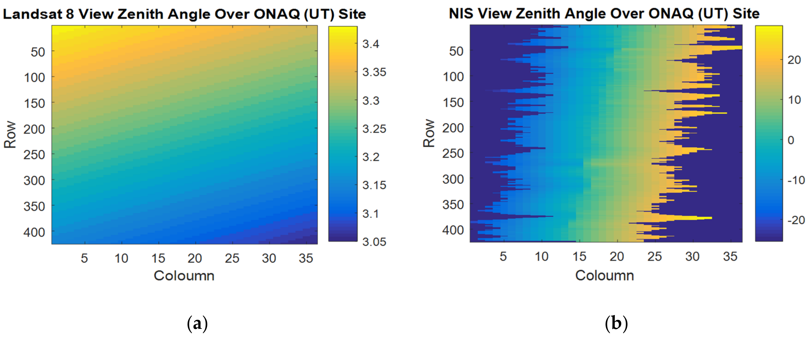
The bidirectional reflectance distribution function (BRDF) describes how SR varies with geometries such as view zenith angle (VZA), solar zenith angle (SZA) and azimuth angles [55]. The main discrepancy in the observing geometries between OLI and NIS sensors was in the view angles ranges between both sensors. Figure 13 shows a comparison between OLI VZA and NIS VZA over the Onaqui-Ault (ONAQ) (UT) site.
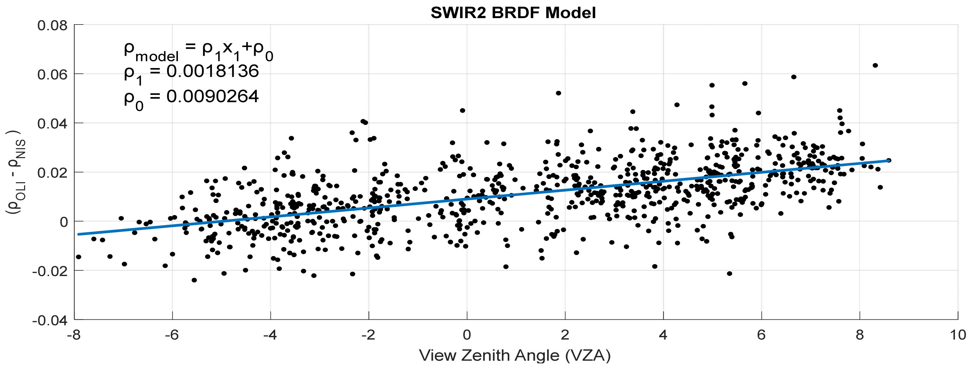
From Figure 13, OLI VZA exhibited variation of only 3.05° to 3.4°, whereas, the NIS VZA ranged from –25° to 25°, over the same area. Governed by the surface and the spectral band, differences in viewing geometry will likely result in the introduction of a BRDF effect [56]. Since scattering and directional reflectance effects varies with wavelength and cover type, individual BRDF models were created for all NEON sites and each NIS band. The NIS BRDF models did not account for solar geometry due to the lack of changes in the solar zenith angles between the sensor overpasses at the selected NEON sites. For the ONAQ site, the OLI and NIS solar zenith angles were 25° and 26° respectively. Figure 14 shows the resulting model for the SWIR2 band applicable to the ONAQ (UT) NEON site.
The BRDF model, from Figure 14, approximated the relationship of the observed SR difference between OLI and NIS, at the corresponding NIS VZA:
where, is the model predicted reflectance difference for a given pixel at the corresponding NIS VZA. The BRDF correction was accomplished by using the difference model in Equation (8) to normalize the OLI and NIS SR differences measurements to one common OLI VZA “reference” geometry:
where, is the observed reflectance difference for a given pixel at the corresponding VZA and is the “reference” predicted reflectance difference as a function of the reference VZA (mean OLI VZA within the ROI). The BRDF correction () from Equation (9) was applied to each NIS ROI (from Table 3). The BRDF corrected NIS SR for a given pixel was obtained as follows:
The Validation of the OLI L2 product using the BRDF-corrected NIS SR () data followed the same analysis procedure described in Section 2.1.3 for the ground truth measurements.
3. Results and Discussion
After applying all corrections explained in Section 2 on the ground truth measurements and the NIS derived SR, the OLI L2 SR product was validated using both techniques.
3.1. Results of L8 OLI Validation Using Ground Truth Measurements
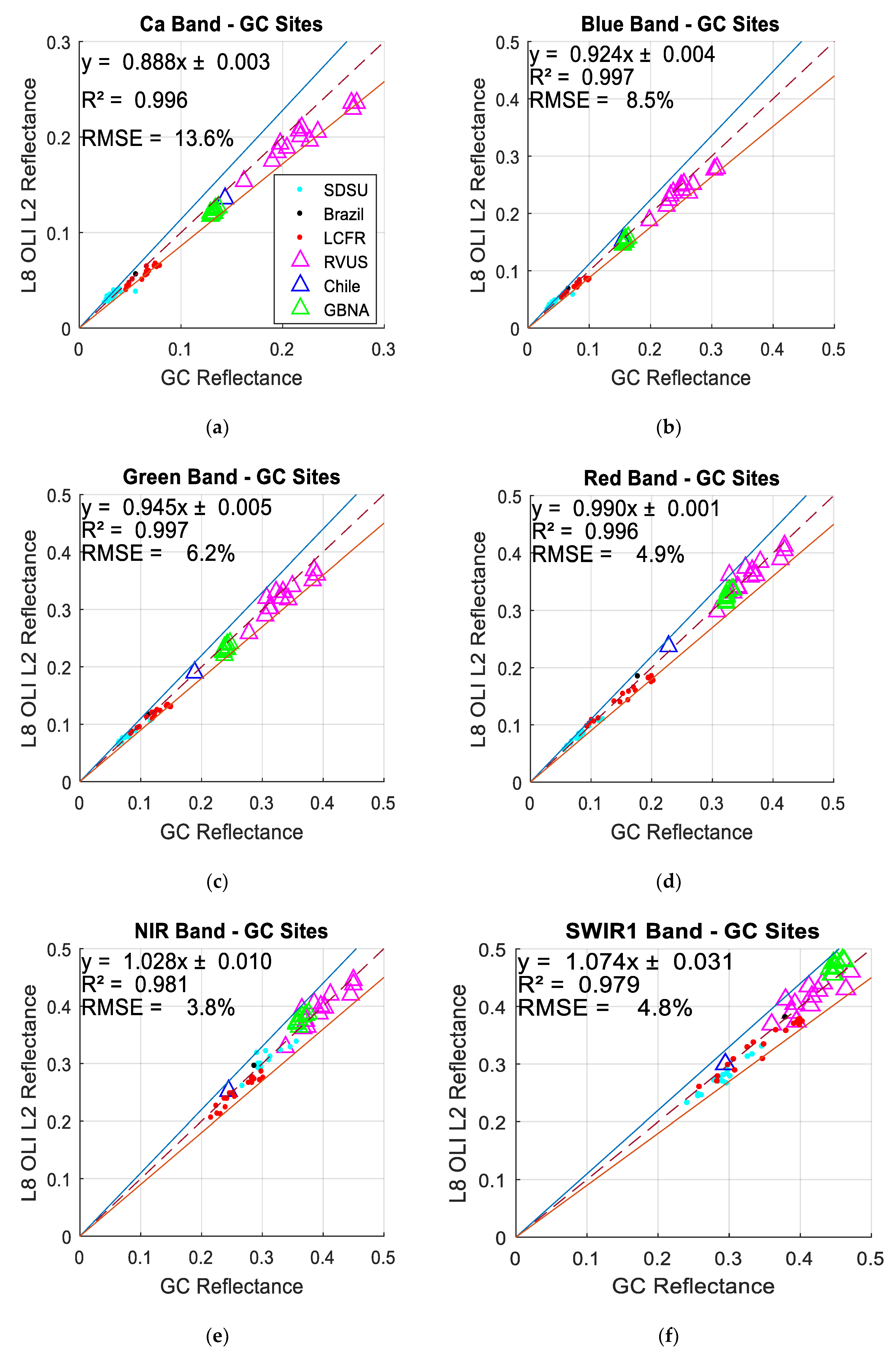
The first method considered to validate the OLI L2 SR product was using direct ground truth measurements. Figure 15a–g shows the scatter plots of the ground truth reflectance vs. OLI L2 surface reflectance, over the six sites reported in Table 2. The dashed lines in each Figure represent 1:1 lines used as reference; the solid lines indicate the uncertainty regions for the OLI L2 surface reflectance product (approximately ±10%) [44]. The bright sites are represented by a triangle, whereas, the circles represent vegetation sites. A linear regression could then be calculated to represent the differences between OLI derived surface reflectance and ground truth measured reflectance. The correlation coefficient (R2) and the root mean square error (RMSE) were also computed per band.
The ground truth validation attempt of OLI L2 SR product showed high agreement with ground truth reflectance measurements across all bands, as indicated by the estimated R2 values of 0.98 or higher. Over 90% of the data points for all bands fall within the OLI’s SR product stated 10% uncertainty [44].
The visible bands exhibited the largest differences between the OLI L2 SR and GC measurements. Some of the LCFR CA and Blue bands data falls just outside of the estimated uncertainty, the OLI L2 SR product at the CA and Blue bands displayed greater deviation from the 1:1 line with RMSE percentages of approximately 13.6% and 8.5%, respectively. The ground truth validation of OLI L2 SR product is more accurate in the longer wavelength bands. All the data points fall closer to the 1:1 line, particularly in the NIR and SWIR1 bands, they all had similar behavior with the lowest RMSE percentages of approximately 3.8% and 4.8%, respectively. The OLI L2 SR product is more accurate in these bands and is consistent across different cover types (soil and vegetation), under different atmospheric conditions.
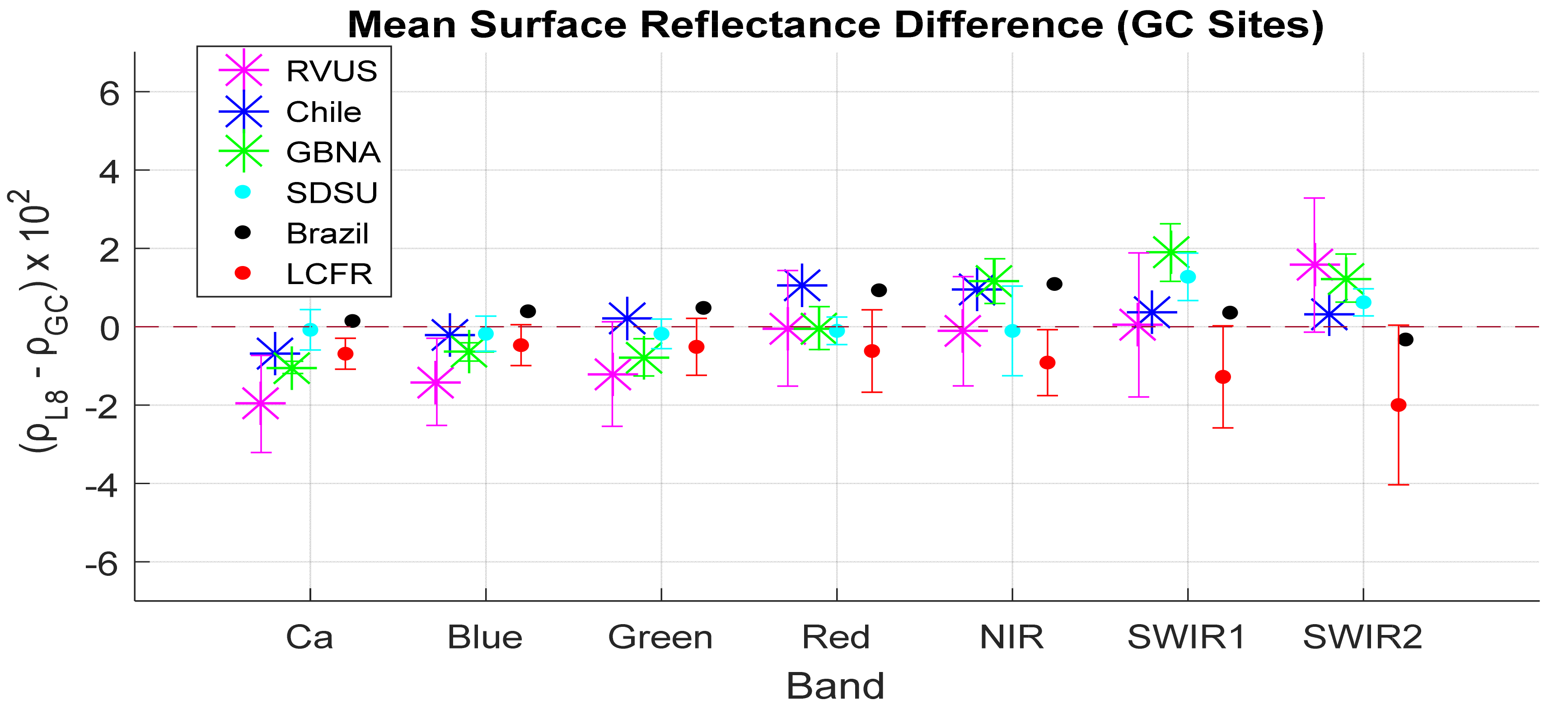
Figure 16 shows the mean reflectance difference (expressed in percentage) and the 1σ standard deviation of the ratio between the site-specific measured ground truth reflectance and observed OLI L2 SR obtained during the corresponding six field campaign measurements. The mean reflectance difference was used to describe the bias of OLI L2 product: negative if OLI SR is underestimated, and positive if OLI SR is overestimated. A smaller mean reflectance difference magnitude represents a better agreement between the OLI L2 SR product and ground truth measurements.
Figure 16 demonstrates that the validation attempt using ground truth reflectance measurements shows good consistency with the OLI derived L2 SR, with a bias less than ±2% across all bands and sites. The Green, Red and NIR bands tend to have a mean reflectance differences averaging approximately ±1% or less for all bright and vegetation targets at the ground truth sites. In the shorter wavelengths, the mean reflectance difference across all sites is highest at the RVUS site, with a reflectance difference of approximately –2% and –1.5% in the CA and Blue bands respectively. Whereas in the longer wavelengths, OLI had a mean reflectance difference of approximately 2% in the SWIR1 band over GBNA, and –2% mean reflectance difference over LCFR in the SWIR 2 band.
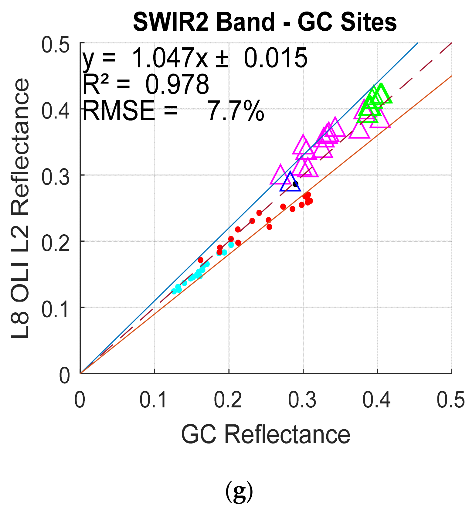
The OLI L2 SR product validation was within the stated uncertainty region of 10% in the Blue-SWIR2 bands, which indicates a consistent result with truth estimates at the ground level. Retrieval at the CA band was the most troublesome as indicated by the RMSE of 13.6%. The larger differences observed in the CA, and to a less extent the Blue band, are primarily due to difficulties in aerosol estimation and lower signal levels received by the OLI [57,58]. The validation of the OLI in the Green and Red bands exhibited less deviation and falls within the L2 uncertainty region, with an RMSE percentage of approximately 6.2% and 4.9% respectively. Whereas, at the longer wavelengths, the atmospheric transmittance is typically higher, resulting in a higher measured reflectance level, and atmospheric effects tend to be minimal. The agreement in these bands is consistent across different cover types (soil and vegetation) and atmospheric conditions. Some of the LCFR and RVUS data in the SWIR2 band falls just outside of the estimated uncertainty, and this primarily is due to the effects of water vapor absorption which dominates the SWIR spectral region [59].
The validation results of the OLI L2 SR product varied spectrally across vegetation and bright sites. Therefore, further analysis was performed to validate the product. Table 4 shows the RMSE and the 1σ standard deviation (expressed in percent) of the ratio between the observed OLI L2 SR and the ground truth site-specific measurements for RVUS, GBNA, SDSU and LCFR. The RMSE and standard deviations of Chile and Brazil sites were not included in Table 4 because there was only one OLI overpass per site. The largest differences were observed in the SWIR2 band at the RVUS and LCFR sites with RMSEs of 2.27% and 2.81% and a standard deviations of 1.71% and 2.03% respectively.
In the CA and Blue bands from Figure 15a,b, the OLI L2 SR product showed good agreement with ground truth measurements of 0.1 SR or less. Reflectance at that level is associated with the vegetation dominant sites: SDSU, LCRF and Brazil. The RMSE (from Table 4) for the SDSU and LCFR sites are less than 0.79%, with a standard deviation of ~0.5%. SRs larger than 0.1 are associated with the bright sites: RVUS, GBNA, and Chile. The GBNA bright site showed more linear agreement between the OLI L2 SR product and ground truth measurements, with an RMSE of 1% and a standard deviation of 0.12. Whereas, the RVUS bright site showed more scatter and variation between the OLI L2 SR and ground truth measurements, with an RMSE of 2.3% and a standard deviation of 1.2%.
In the Green and Red bands from Figure 15c,d, the SR between the OLI SR and ground truth measurements over the SDSU site showed similar agreement, with an RMSE on the order of 0.41% and variation of 0.38% or less. However, the LCRF site showed more variation and scatter than SDSU, as shown by the larger standard deviation of 1.05%. The RVUS and GBNA sites indicated a better agreement between OLI and ground truth data points, in the Green and Red bands than they did in CA and Blue bands, with an RMSE of 1.42% and 0.51% respectively. Nevertheless, the OLI L2 SR product over all three bright sites in the CA -Green bands, are generally lower than the ground truth measurements. This result suggests that there is a potential aerosol overestimation by LaSRC in deriving the OLI L2 product, mainly due to the difficulties of atmospheric characterization in the CA and Blue bands.
In the NIR band shown in Figure 15e, the OLI L2 SRs within 0.2–0.3 at the LCFR site are generally lower than ground truth measurements. The SDSU, LCFR and RVUS sites exhibited similar scatter, with standard deviations of 1.14%, 0.84% and 1.39% respectively. On the other hand, the performance of the OLI L2 product at the GBNA bright sites is more precise as shown by the variation of only 0.56%. The measurements at the GBNA site indicates a higher SR estimate observed by the OLI L2 SR product than the ground truth measurements with an RMSE of 1.28%.
The SWIR1 band in Figure 15f showed that the SR retrievals over vegetation sites were lower than the ground truth measurements. This was indicated with RMSEs of 1.4% and 1.8% for the SDSU and LCFR sites respectively. Shown in Figure 15g, the OLI SR had the largest difference from ground truth measurements of 2.81% RMSE at the LCFR site in the SWIR2 band with a variation of 2.03%. Whereas, OLI demonstrated a consistent agreement with ground truth measurements with an RMSE of 0.7% and a variation of 0.34% at the SDSU site. The OLI L2 SR product over the bright sites in the SWIR bands were higher than the ground truth measurements, showing a clear, high bias, driven largely by the GBNA site, with an RMSE of 2.01% in the SWIR1 band.
Generally, the RVUS and LCFR sites showed the most spread and variation between OLI and ground truth measurements across all bands, with a standard deviation varying from 1.1% to 1.84% for the RVUS site and 0.39%–2.03% for the LCFR site. For vegetated cases, retrievals at the SDSU site provided a closer match to the ground truth measurements, and also recorded a wide range of SRs from 0 to 0.4. Consistency between the OLI L2 SR product and ground truth measurements at the SDSU site can be seen in the VIS and SWIR bands with standard deviations less than 0.59%, whereas, a larger spread and variation of 1.14% from ground truth measurements was observed in the NIR band. Finally, the OLI L2 SR product values retrieved from the GBNA bright site seems to be in agreement with the ground truth measurements across all bands. The variations between the OLI L2 and ground truth measurements at the GBNA site were less than 0.71%. Thus, the GBNA site exhibits the most accurate ground truth SR retrieval for the validation of the OLI L2 SR product.
The OLI L2 SR product bias was measured for vegetation and bright covers. Table 5 shows the mean reflectance differences and standard deviations, expressed as percentages, for the combined vegetation sites (SDSU, Brazil and LCFR), combined bright sites (RVUS, Chile, and GBNA). In general, the estimated mean reflectance difference between the OLI L2 SR product and ground truth measurements indicated a bias of less than 1.24% or less for all sites across all bands.
For the vegetation sites, the mean reflectance differences across all bands are approximately 0.57% or less in magnitude. The differences in the VNIR bands are approximately 0.21% or less in magnitude, with the larger bias observed in the SWIR bands. There appears to be greater variability between the OLI L2 product and ground truth measurements as the wavelength increases, ranging from a minimum standard deviation of approximately 0.43% in the CA band to a maximum of approximately 1.3% in the SWIR bands. For the bright sites, the mean reflectance differences tended to be somewhat larger and the overall variability somewhat smaller than the vegetation sites, as indicated by the lower mean reflectance differences and larger standard deviations. The mean reflectance differences across all bands ranged between approximately 0.33% and 1.2% in magnitude, while the standard deviations were approximately 0.98% or less.
3.2. Discussion of L8 OLI Validation Using Ground Truth Measurements
The best path for surface reflectance validation is by using ground truth measurements, due to its direct traceability and high accuracy of 2% for ground campaign field measurements [16] and 3%~4% for RadCalNet measurements [22]. The overall results of the ground truth validation of the L8 OLI L2 SR product was considered on aggregate, by combing the mean reflectance differences of all sites across all bands. Table 6 shows the mean reflectance differences and standard deviations, expressed as percentages, for the six ground truth sites combined.
When considering the combined ground truth data from Table 6, the overall validation estimate shows that the OLI L2 SR product is off, at the most, by a mean reflectance difference level of 0.81% ± 0.97% which encompasses the ground truth uncertainty values. Thus, this result indicates that the OLI L2 SR product is in consistent agreement with truth measurements across all the bands and sites. The largest negative bias of 0.51% ± 0.93% was observed in the CA band, whereas, the largest positive bias of 0.81% ± 0.97% was in the SWIR2 band. This result is expected, due to the larger effects of aerosols and water vapor effects in the CA and SWIR2 bands respectively. However, the OLI L2 product reflectances are consistently less than the ground truth measurements at shorter wavelengths and consistently greater at longer wavelengths. Differences in the shorter wavelength is possibly due to the excessive aerosol being estimated and inputted into the LaSRC algorithm, primarily developed to transform TOA reflectance to SR [9,40], thus the retrieved SR is underestimated. Whereas, at longer wavelengths, the SR is being overestimated, predominantly due to the spatial and temporal variability of water vapor, which makes it more difficult to quantify. Furthermore, water vapor can only be directly estimated from satellite data if there is a designated water vapor absorption channel [60]. Thus, LaSRC relies on auxiliary data to perform the necessary corrections [61,62].
3.3. Results of L8 Validation Using NEON Imaging Spectrometer (NIS) SR
The second method of the OLI L2 SR validation was based on the multispectral, geometrically and spatially corrected NIS SR, as described in Section 2.2. Comparison of OLI SR to NIS SR was based on homogeneous ROIs selected as shown in Table 3.
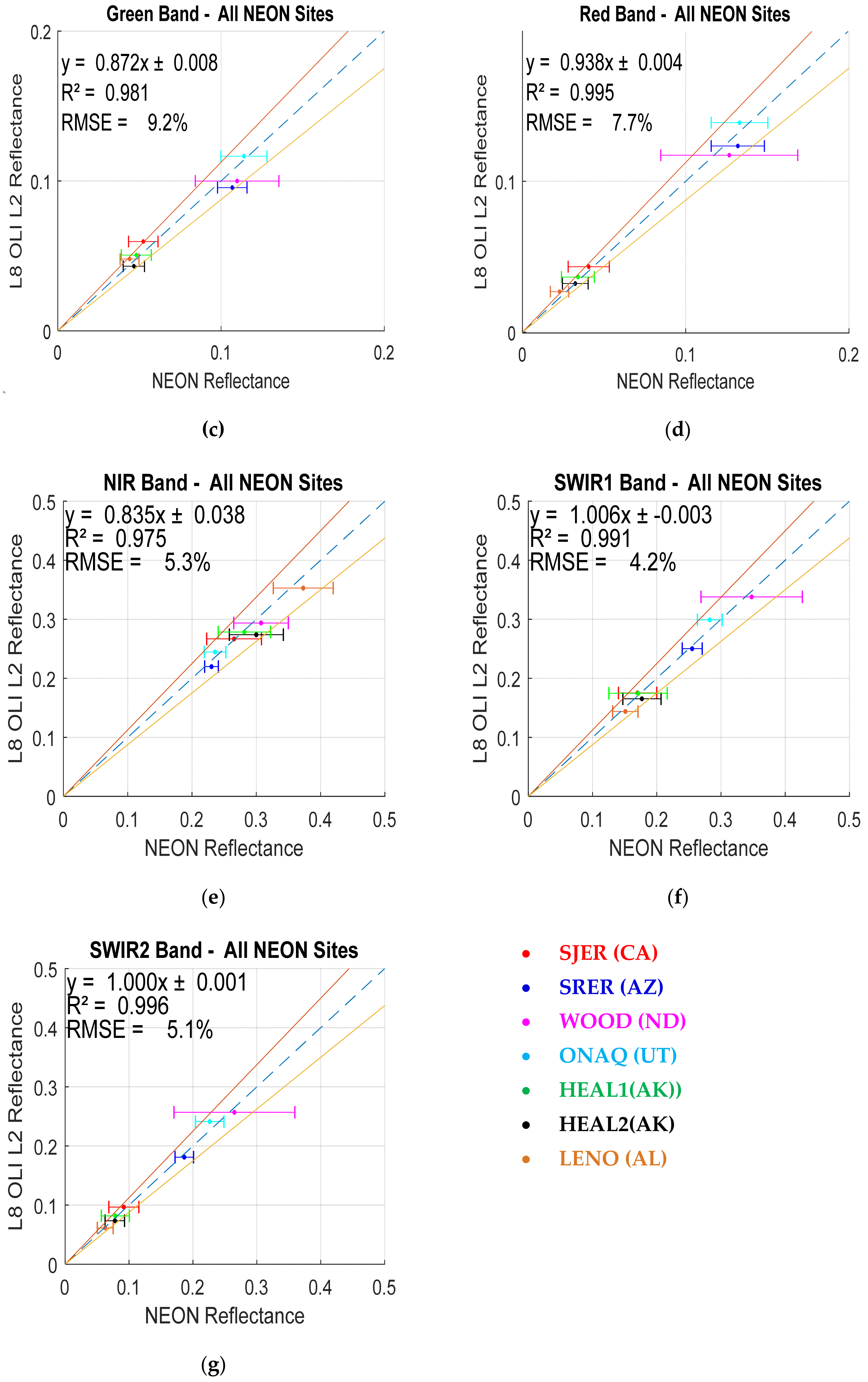
Figure 17a–g shows the scatterplots of OLI L2 SR vs. NIS SR that were averaged across all sites. The NIS product is subject to an uncertainty of 5%–10% [30]. The dashed lines in each Figure represents the 1:1 line used as reference; the solid lines indicate the uncertainty regions for the NIS and OLI L2 surface reflectance product, (approximately ±15%). NEON is subject to a higher uncertainty since the measurements are acquired at ~1000 m above the surface and have been corrected to surface reflectance. The error bars represent the 1σ standard deviation of the mean NIS reflectance across the ROI for each site. The comparison of NIS and OLI surface reflectance values for all dates at all locations exhibit a high degree of positive correlation between the two data sets, with R2 values of approximately 0.9 or greater.
As might be expected, the validation of OLI L2 SR using NIS SR is least accurate in the VIS bands, which is indicated by the estimated RMSE estimates in the CA, Blue, and Green bands of 31.7%, 17.3%, and 9.2%, respectively. The CA and Blue band estimates do not fall within the expected ~15% product uncertainty and the majority of data points are located outside of the uncertainty region. The Green and Red bands appear to exhibit greater accuracy at all sites except for the Lenoir Landing (LENO) (AL) site, whose estimates fall outside of the expected uncertainty range in all visible bands. This is due to surface reflectance measurements of 0.05 or less, which are more sensitive to aerosol loading in the atmosphere. In the Red, NIR, SWIR1 and SWIR 2 bands, signal levels are higher. The OLI L2 product surface reflectances across all sites fall within the expected 15% uncertainty range, generally following the 1:1 trend, as shown by the lower RMSE values of approximately 7.7%, 5.3%, 4.2% and 5.1%, respectively.
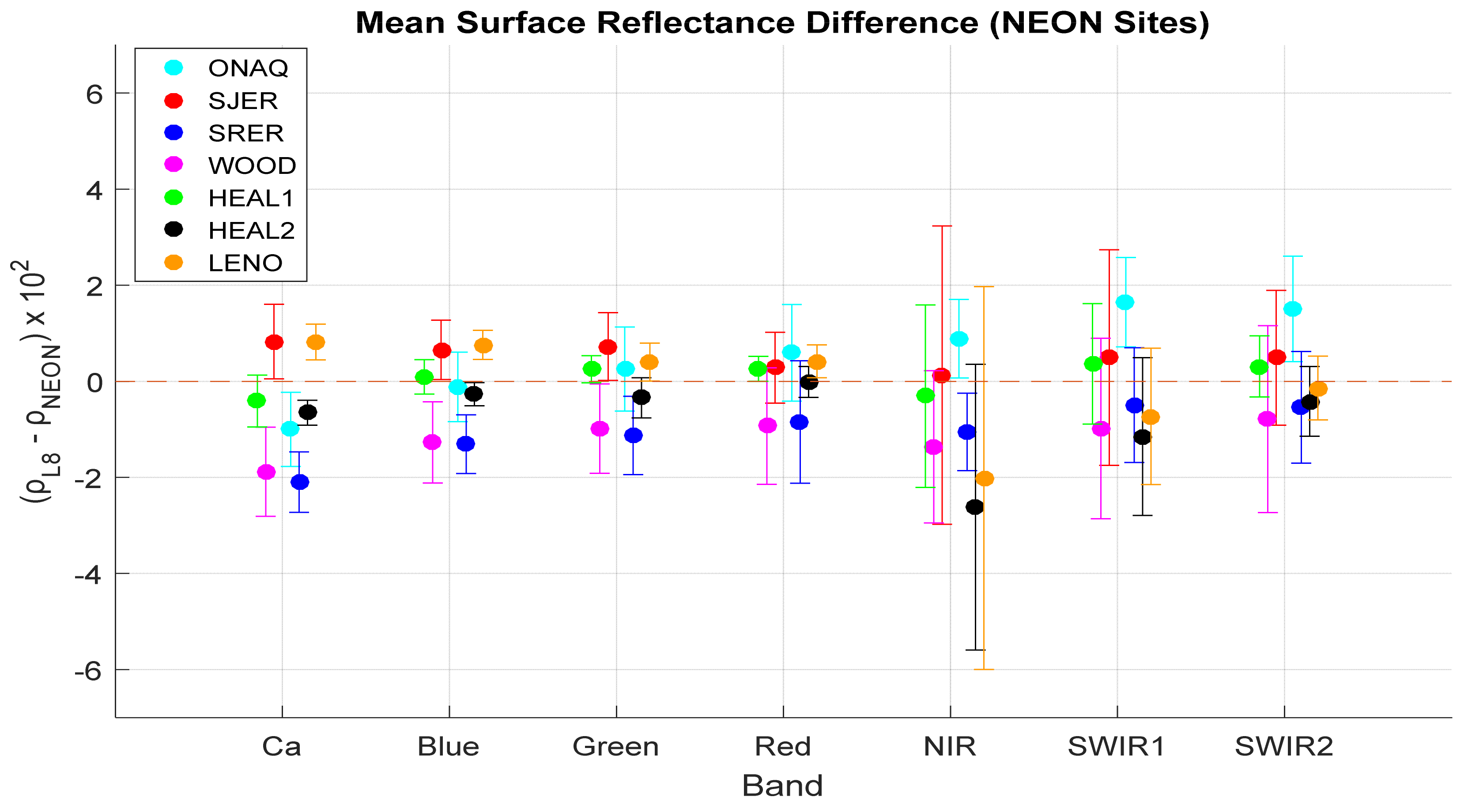
Figure 18 shows the mean reflectance difference estimates of the OLI L2 SR using NIS derived SR to estimate the bias. The error bars represent the 1σ standard deviation of the ratio between the site-specific measured NEON reflectance and observed OLI L2 SR reflectances obtained during the corresponding airborne measurements. In general, validation of the OLI L2 products against the NIS SR products exceeded expectations, given the reported 10% uncertainty for the OLI products and 5%–10% uncertainty for the NIS products.
Overall, the initial validation attempts of the OLI L2 SR product using the NIS resulted in a low bias of ±2.5% or less across all bands, showing similar results with the previous validation attempt using ground truth results. For the NIR band, the sites LENO and Healy (HEAL2) had the largest mean reflectance difference of –2.5% and –2% respectively. Those sites had the largest variation as shown by their standard deviations of 3.98% and 2.97% respectively. The main cause of variation can be attributed to nearby shadow effects in HEAL and Woodworth (WOOD), which was reported to be over 50% [63]. Thus, in such cases, directional effects and adjacency effects are more important, which tends to cause larger deviations between OLI and NIS [64].
3.4. Discussion of L8 Validation Using NEON Imaging Spectrometer (NIS) SR
To account for scale differences between OLI and NIS, a data matching procedure was performed on the NIS SR measurements to accurately validate the OLI L2 SR product. As described in Section 2.2.2 the following was accounted for: (i) the spectral response of both sensors, (ii) image mis-registration, (iii) the spatial averaging of the NIS pixels and (iv) differences in the sensor viewing angles between the OLI and NIS (the NIS images were not acquired at a nadir view).
The OLI L2 SR validation was further validated using vegetative cover at a total of six NEON sites. The CA and Blue bands were off the expected uncertainty by an order of 31% and 17.3% RMSE. The primary cause of this discrepancy between OLI L2 and NIS SR values was most likely due to the atmospheric effects. Predominantly, the CA and Blue bands are heavily affected by the aerosols, which contributes to an increase in the path radiance seen by the sensor due to the Rayleigh scattering effects. Furthermore, LASRC seems to underestimate aerosols correction at the CA and Blue bands, reflectance at six out of seven sites seems to be lower in OLI than NIS SR measurements. Given the calibration uncertainties of OLI and NIS sensors, and necessary atmospheric corrections to derive the SR, the OLI L2 SR product is subject to an uncertainty of ~10%, and an additional 5%–10% uncertainty can be expected from the NIS sensor. Therefore, the largest differences from truth measurements are present in the CA and Blue bands.
The Green-SWIR2 bands of the OLI L2 SR product were all within the ~15% expected uncertainties and showed consistency with NIS SR measurements on the order of 9% RMSE or less. The Green-SWIR2 bands are subject to less path radiance, and correction of aerosols becomes minimal. Note that the RMSE (%) could be large when a weak linear relationship exists between satellite retrievals and ground data, even if the bias is low. Thus RMSE (expressed as a percentage) is a relatively poor descriptor of accuracy for the NIS vegetative sites, as they all exhibit little dynamic range in the CA and Blue bands. In this case combining the mean reflectance differences and standard deviations, expressed as percentages, for all the NEON sites used in the validation analysis of OLI L2 SR product is a better indicator of validation. Table 7 shows the OLI L2 SR combined mean reflectance differences estimates, with all NEON sites combined.
The NIS SR validates the OLI L2 SR product to the 1.0% level mean reflectance difference across all bands, with a standard deviation of less than 1.25%. This result shows a significant improvement in the mean reflectance difference, especially in the NIR band, going from –2.5% in the LENO site to –0.91% on average across all sites. Thus, averaging the mean reflectance differences between NEON and OLI L2 SR across all the sites in Table 3 produces a significantly better validation assessment to the OLI L2 SR product, than validating the product with individual NEON sites.
The results of this evaluation indicate that SR derived from the NEON on-board NIS sensor can be used with confidence to provide an alternative method to accurately validate SR measurements, especially in the VNIR bands. In the SWIR bands, the validation attempt using NIS SR estimated lower mean reflectance differences than those estimated by the ground truth validation method. Since ground truth is a more direct and accurate validation method than NIS, it is not advised to use the NIS SR to validate in the infrared bands.
4. Conclusions
The validation of the Landsat 8 OLI L2 SR product was performed using two methods: (i) OLI L2 product validation using direct surface reflectance measurements; (ii) OLI L2 product validation using SR derived from AOP operated by NEON, corrected to match OLI geometry, spatial and spectral resolutions. Ground truth data has the capability of producing direct surface reflectance at the 2% level for ground campaigns and 3%~4% for RadCalNet [22]. This provides the most accurate method to validate surface reflectance products. Due to the limited availability of truth measurements, NIS validation was considered, which is capable of producing SR at the 5%–10% level [30].
When considering the ground truth data, the results indicate that the OLI SR product is validated at the mean reflectance difference levels of ±0.81% (0.0081 units of reflectance), across all bands and sites. The largest differences between the OLI and ground truth measurements were mainly observed at the shorter wavelengths, specifically the CA and Blue bands, with mean reflectance differences of ±1.2% and ±0.8%, respectively. Percent difference across the CA band was outside of the expected uncertainty on the order of 13.6% RMSE. The Blue bands percent difference was just within the expected uncertainty on the order of 9% RMSE. Therefore, initial efforts to validate the OLI L2 SR product suggest there are more difficulties in SR retrieval at the CA and Blue bands, especially over dense dark vegetation targets. This is attributed to a potential LaSRC aerosols overcorrection at the CA and Blue bands, SRs at six out of seven sites seem to be smaller in OLI than ground truth measurements.
The OLI validation using NIS SR indicated that the SR derived from the NEON on-board NIS sensor can be used with confidence to provide an alternative method to accurately validate SR measurements, especially in the VNIR. The OLI validation using NIS derived SR was consistent with validation using ground truth measurements in the VIS bands, with NIS reporting larger RMSE percentages on the order of 31.7%, 17.3%, 9.2% and 7.7%. However, NIS reported lower RMSE in the SWIR bands (4.2% and 5.1% respectively). Since ground truth validation is more accurate and provides a more direct validation of SR than airborne measurements, it is not recommended to validate the SWIR band of OLI L2 SR product using derived NIS SR products. The mean reflectance difference estimates between the OLI L2 SR product and NIS SR showed variation across all seven NEON sites and bands, with a bias larger than 2% in magnitude.. However, on average, the seven NEON sites resulted in a bias of less than ~1% between OLI L2 SR and NIS SR, which is consistent with the direct surface reflectance validation bias estimates.
Considering both validation methods to validate the OLI L2 SR product, the reflectance dynamic range detected by OLI varied from 0 to 0.5 across all bands. Over that range, the results indicate that the OLI SR is validated at the mean reflectance difference levels of ±0.91% (0.0091 units of reflectance) across all bands and all 13 sites. The OLI L2 SR product validation was more accurate in the longer wavelengths. As a measure of overall difference from the “truth” measurements, the RMSE across the Green-SWIR2 bands between the OLI and ground truth/NIS validation techniques was less than 9%. Bias in the OLI L2 SR product retrievals from ground truth estimates was ±0.63% (0.0063 units of reflectance) or less for the Green-SWIR2 bands. These results are well within the associated uncertainties of the L2 validation methods used (~10% for ground truth and 15% for NIS). The possible overcorrection in the Landsat surface reflectance due to the variant nature of water vapor at the SWIR bands might contribute to the positive bias value. On the other hand, more difficulties were noted in the OLI L2 SR retrieval in the CA band as indicated by the ground truth RMSE of 13.6% and NIS RMSE of 31.7% which was not within the expected uncertainty of the OLI L2 SR product.
Author Contributions
Conceptualization and design, M.B., D.H., L.L, X.J.; methodology, M.B.; RCN Data Processing, X.J, L.L., M.B.; software, M.B.; validation, M.B.; formal analysis, M.B.; resources and support, D.H., L.L.; writing—All drafts, M.B; writing—Review and editing, D.H, L.L., visualization, M.B.; supervision, D.H., X.J., L.L.
Acknowledgments
The authors would like to thank all colleagues and staff members at the SDSU image processing laboratory for their thoughtful comments that improved this research. The authors would like to thank Tim Ruggles for his extensive technical writing correction. The authors would also like to thank NASA and USGS, RadCalNet and NEON for providing Landsat8, automated Ground truth measurements, and NEON Imaging spectrometer data. Last but not least, we enthusiastically recognize all the reviewers for their vital comments and recommendations for refining the manuscript. This research was supported by NASA grant number NNX15AP36A and USGS grant number G14AC00370.
Conflicts of Interest
The authors declare no conflict of interest. The funders had no role in the design of the study; in the collection, analyses, or interpretation of data; in the writing of the manuscript, or in the decision to publish the results.
References
- Feng, M.; Huang, C.; Channan, S.; Vermote, E.F.; Masek, J.G.; Townshend, J.R. Quality assessment of Landsat surface reflectance products using MODIS data. Comput. Geosci. 2012, 38, 9–22. [Google Scholar] [CrossRef] [Green Version]
- Radiometric Calibration and Corrections. Available online: http://gsp.humboldt.edu/OLM/Courses/GSP_216_Online/lesson4-1/radiometric.html (accessed on 7 October 2018).
- Qian, Y.; Wang, N.; Ma, L.; Liu, Y. Vicarious radiometric calibration/validation of Landsat-8 operational land imager using a ground reflected radiance-based approach with Baotou site in China. J. Appl. Remote Sens. 2017, 11, 044004. [Google Scholar]
- Markham, B.L.; Helder, D.L. Forty-year calibrated record of earth-reflected radiance from Landsat: A review. Remote Sens. Environ. 2012, 122, 30–40. [Google Scholar] [CrossRef] [Green Version]
- Roy, D.P.; Wulder, M.A.; Loveland, T.R.; Woodcock, C.E.; Allen, R.G.; Anderson, M.C.; Helder, D.; Irons, J.R.; Johnson, D.M.; Kennedy, R.; et al. Landsat-8: Science and product vision for terrestrial global change research. Remote Sens. Environ. 2014, 145, 54–172. [Google Scholar] [CrossRef]
- USGS-EROS/espa-surface-reflectance. [Product Guide] December 2018. Available online: https://github.com/USGS-EROS/espa-surface-reflectance/tree/master/lasrc (accessed on 14 September 2018).
- USGS-EROS LaSRC Version 1.4.1 Release Notes. Available online: https://github.com/USGS-EROS/espa-surface-reflectance/tree/master/lasrc (accessed on 2 November 2018).
- Dwyer, J.L.; Roy, D.P.; Sauer, B.; Jenkerson, C.B.; Zhang, H.K.; Lymburner, L. Analysis Ready Data: Enabling Analysis of the Landsat Archive. Remote Sens. 2018, 10, 1363. [Google Scholar]
- Vermote, E.F.; El Saleous, N.; Justice, C.O.; Kaufman, Y.J.; Privette, J.L.; Remer, L.; Roger, J.C.; Tanré, D. Atmospheric correction of visible to middle-infrared EOS-MODIS data over land surfaces: Background, operational algorithm and validation. J. Geophys. Res. Atmos. 1997, 102, 17131–17141. [Google Scholar] [CrossRef] [Green Version]
- Zhang, H.K.; Roy, D.P.; Yan, L.; Li, Z.; Huang, H.; Vermote, E.; Skakun, S.; Roger, J.-C. Characterization of Sentinel-2A and Landsat-8 top of atmosphere, surface, and nadir BRDF adjusted reflectance and NDVI differences. Remote Sens. Environ. 2018, 215, 482–494. [Google Scholar] [CrossRef]
- SDState Image Processing Lab. Available online: https://www.sdstate.edu/jerome-j-lohr-engineering/engineering-research/image-processing-lab (accessed on 15 May 2018).
- Radiometric Calibration Network Portal. Available online: https://www.radcalnet.org/#!/ (accessed on 20 December 2018).
- Czapla-Myers, J.; McCorkel, J.; Anderson, N.; Thome, K.; Biggar, S.; Helder, D.; Aaron, D.; Leigh, L.; Mishra, N. The Ground-Based Absolute Radiometric Calibration of Landsat 8 OLI. Remote Sens. 2015, 7, 600–626. [Google Scholar] [CrossRef] [Green Version]
- Maiersperger, T.K.; Scaramuzza, P.L.; Leigh, L.; Shrestha, S.; Gallo, K.P.; Jenkerson, C.B.; Dwyer, J.L. Characterizing LEDAPS surface reflectance products by comparisons with AERONET, field spectrometer, and MODIS data. Remote Sens. Environ. 2013, 136, 1–13. [Google Scholar] [CrossRef] [Green Version]
- Anderson, N.; Biggar, S.F.; Burkhart, C.J.; Thome, K.J.; Mavko, M. Bidirectional calibration results for the cleaning of Spectralon reference panels. Int. Symp. Opt. Sci. Technol. 2002, 484, 201–211. [Google Scholar]
- Helder, D.; Thome, K.; Aaron, D.; Leigh, L.; Czapla-Myers, J.; Leisso, N.; Biggar, S.; Anderson, N. Recent surface reflectance measurement campaigns with emphasis on best practices, SI traceability and uncertainty estimation. Metrologia 2012, 49, S21–S28. [Google Scholar] [CrossRef] [Green Version]
- Jackson, R.D.; Moran, M.S.; Slater, P.N.; Biggar, S.F. Field calibration of reference reflectance panels. Remote Sens. Environ. 1987, 22, 145–158. [Google Scholar] [CrossRef]
- Biggar, S.F.; Thome, K.J.; Wisniewski, W. Vicarious radiometric calibration of EO-1 sensors by reference to high-reflectance ground targets. IEEE Trans. Geosci. Remote Sens. 2003, 41, 1174–1179. [Google Scholar] [CrossRef]
- Thome, K.J. Absolute radiometric calibration of Landsat 7 ETM+ using the reflectance-based method. Remote Sens. Environ. 2001, 78, 27–38. [Google Scholar] [CrossRef]
- RadCalNet Quick Start Guide. Available online: https://www.radcalnet.org/resources/RadCalNetQuickstartGuide_20180702.pdf (accessed on 2 July 2018).
- Czapla-Myers, J.; Ong, L.; Thome, K.; McCorkel, J. Validation of EO-1 Hyperion and Advanced Land Imager Using the Radiometric Calibration Test Site at Railroad Valley, Nevada. IEEE J. Sel. Top. Appl. Earth Obs. Remote Sens. 2016, 9, 816–826. [Google Scholar] [CrossRef]
- Czapla-Myers, J.S.; Thome, K.J.; Leisso, N.P. Radiometric calibration of earth-observing sensors using an automated test site at Railroad Valley, Nevada. Can. J. Remote Sens. 2014, 36, 474–487. [Google Scholar] [CrossRef]
- National Center for Atmospheric Science (Sun Photometer). Available online: https://www.ncas.ac.uk/en/cimel-sun-photometer (accessed on 7 March 2019).
- Ong, C.; Thome, K.; Heiden, U.; Czapla-Myers, J.; Mueller, A. Reflectance-Based Imaging Spectrometer Error Budget Field Practicum at the Railroad Valley Test Site, Nevada [Technical Committees]. IEEE Geosci. Remote Sens. Mag. 2018, 6, 111–115. [Google Scholar] [CrossRef] [Green Version]
- Kuester, M.; Thome, K.J.; Biggar, S.F.; Krause, K.S. Solar-radiation-based calibration of an airborne radiometer for vicarious calibration of earth observing sensors. In Proceedings of the International Symposium on Optical Science and Technology, San Diego, CA, USA, 29 July–3 August 2001; Volume 4483. [Google Scholar]
- Thome, K.; Amico, J.D.; Hugon, C. Intercomparison of Terra ASTER, MISR, and MODIS, and Landsat-7 ETM+. In Proceedings of the 2006 IEEE International Symposium on Geoscience and Remote Sensing, Denver, CO, USA, 31 July–4 August 2006. [Google Scholar]
- Biggar, S.; Anderson, N.; McCorkel, J.; Czapla-Myers, J. Earth-observing satellite intercomparison using the Radiometric Calibration Test Site at Railroad Valley. J. Appl. Remote Sens. 2017, 12, 012004. [Google Scholar]
- Czapla-Myers, J.S.; Thome, K.J.; Leisso, N.P. Calibration of AVHRR sensors using the reflectance-based method. In Proceedings of the Optical Engineering + Applications, San Diego, CA, USA, 26–30 August 2007; Volume 6684. [Google Scholar]
- Airborne Remote Sensing. Available online: https://www.neonscience.org/data-collection/airborne-remote-sensing (accessed on 12 July 2018).
- Bryan Karpowicz, T.K. Neon Imaging Spectrometer Radiance to Reflectance. Available online: http://data.neonscience.org/api/v0/documents/NEON.DOC.001288vA (accessed on 10 July 2018).
- Types of NEON Field Sites. Available online: https://www.neonscience.org/field-sites/types-neon-field-sites (accessed on 12 December 2018).
- Field Sites List. Available online: https://www.neonscience.org/field-sites/field-sites-map/list (accessed on 12 December 2018).
- Kampe, T.; Gallery, W.; Goulden, T.; Leisso, N.; Krause, K. Neon Imaging Spectrometer Geolocation Processing. 2016. Available online: http://data.neonscience.org/api/v0/documents/NEON.DOC.001290vC (accessed on 14 December 2018).
- Johnson, B.R.; Kampe, T.U.; Kuester, M. Development of airborne remote sensing instrumentations for NEON. In Proceedings of the SPIE Optical Engineering + Applications, San Diego, CA, USA, 1–5 August 2010; Volume 7809. [Google Scholar]
- Kampe, T.; Leisso, N.; Musinsky, J.; Petroy, S.; Karpowicz, B.; Krause, K.; Crocker, R.; Devoe, M.; Penniman, E.; Guadagno, T.; et al. The NEON 2013 Airborne Campaign at Domain 17 Terrestrial and Aquatic Sites in California; Battelle Memorial Institute: Boulder, CO, USA, 2014. [Google Scholar]
- Slater, P.N.; Biggar, S.F.; Holm, R.; Jackson, R.G.; Mao, Y.; Moran, M.S.; Palmer, J.M.; Yuan, B. Reflectance-and radiance-based methods for the in-flight absolute calibration of multispectral sensors. Remote Sens. Environ. 1987, 22, 11–37. [Google Scholar] [CrossRef]
- Slater, P.N.; Biggar, S.F.; Palmer, J.M.; Thome, K.J. Unified approach to pre-and in-flight satellite-sensor absolute radiometric calibration. In Advanced and Next-Generation Satellites; International Society for Optics and Photonics: Bellingham, WA, USA, 1995; Volume 2583, pp. 130–142. [Google Scholar]
- Thorne, K.; Markharn, B.; Barker, P.S.; Biggar, S.J.P.E.; Sensing, R. Radiometric calibration of Landsat. Photogramm. Eng. Remote Sens. 1997, 63, 853–858. [Google Scholar]
- Teillet, P.M.; Chander, G. Terrestrial reference standard sites for postlaunch sensor calibration. Can. J. Remote Sens. 2010, 36, 437–450. [Google Scholar] [CrossRef]
- Vermote, E.; Justice, C.; Claverie, M.; Franch, B. Preliminary analysis of the performance of the Landsat 8/OLI land surface reflectance product. Remote Sens. Environ. 2016, 185, 46–56. [Google Scholar] [CrossRef]
- USGS Earth Explorer. Available online: https://earthexplorer.usgs.gov/ (accessed on 19 February 2019).
- Roy, D.P.; Ju, J.; Kline, K.; Scaramuzza, P.L.; Kovalskyy, V.; Hansen, M.; Loveland, T.R.; Vermote, E.; Zhang, C. Web-enabled Landsat Data (WELD): Landsat ETM+ composited mosaics of the conterminous United States. Remote Sens. Environ. 2010, 114, 35–49. [Google Scholar] [CrossRef]
- Landsat8 Spectral Band Viewer. Available online: https://landsat.usgs.gov/landsat/spectral_viewer/bands/Ball_BA_RSR.xlsx (accessed on 16 February 2019).
- Vermote, E.; Justice, C.; Csiszar, I. Early evaluation of the VIIRS calibration, cloud mask and surface reflectance Earth data records. Remote Sens. Environ. 2014, 148, 134–145. [Google Scholar] [CrossRef] [Green Version]
- Vermote, E.F.; Kotchenova, S. Atmospheric correction for the monitoring of land surfaces. J. Geophys. Res. Atmos. 2008, 113. [Google Scholar] [CrossRef]
- Neon Spectrometer Orthorectified Surface Directional Reflectance—Flightline. Available online: https://data.neonscience.org/data-product-view?dpCode=DP1.30006.001 (accessed on 3 May 2019).
- Irons, J.R.; Dwyer, J.L.; Barsi, J.A. The next Landsat satellite: The Landsat Data Continuity Mission. Remote Sens. Environ. 2012, 122, 11–21. [Google Scholar] [CrossRef] [Green Version]
- Intensity-Based Automatic Image Registration. Available online: https://www.mathworks.com/help/images/intensity-based-automatic-image-registration.html (accessed on 21 August 2018).
- Align Multiple Scenes into a Single Image Using Image Registration. Available online: https://www.mathworks.com/discovery/image-registration.html (accessed on 21 August 2018).
- Weisstein, E. Affine Transformation. Available online: http://mathworld.wolfram.com/AffineTransformation.html (accessed on 15 December 2018).
- Gonzalez, R.C.; Woods, R.E.; Eddins, S.L. Digital Image Processing Using MATLAB®, 2nd ed.Gatesmark Publishing: Knoxville, TN, USA, 2010. [Google Scholar]
- Mean Square Error Metric Configuration. Available online: https://www.mathworks.com/help/images/ref/registration.metric.meansquares.html (accessed on 25 August 2018).
- Fowler, M. Perturbation Theory Expresses the Solutions in Terms of Solved Problems. Available online: https://chem.libretexts.org/Bookshelves/Physical_and_Theoretical_Chemistry_Textbook_Maps/Map%3A_Physical_Chemistry_(McQuarrie_and_Simon)/07._Approximation_Methods/7.4%3A_Perturbation_Theory_Expresses_the_Solutions_in_Terms_of_Solved_Problems (accessed on 23 April 2019).
- Styner, M.; Brechbühler,, C.; Székely, G.; Gerig, G. Parametric Estimate of Intensity Inhomogeneities Applied to MRI. IEEE Trans. Med. Imaging 2000, 19, 153–165. [Google Scholar] [CrossRef]
- Barnsley, M.J.; Lewis, P.; Sutherland, M.; Muller, J.P. Estimating land surface albedo in the HAPEX-Sahel southern super-site: Inversion of two BRDF models against multiple angle ASAS images. J. Hydrol. 1997, 188, 749–778. [Google Scholar] [CrossRef]
- Farhad, M.M. Cross Calibration and Validation of Landsat 8 OLI and Sentinel 2A MSI; South Dakota State University: Brookings, SD, USA, 2018. [Google Scholar]
- Doxani, G.; Vermote, E.; Roger, J.-C.; Gascon, F.; Adriaensen, S.; Frantz, D.; Hagolle, O.; Hollstein, A.; Kirches, G.; Li, F. Atmospheric Correction Inter-Comparison Exercise. Remote Sens. 2018, 10, 352. [Google Scholar] [CrossRef]
- Morfitt, R.; Barsi, J.; Levy, R.; Markham, B.; Micijevic, E.; Ong, L.; Scaramuzza, P.; Vanderwerff, K. Landsat-8 Operational Land Imager (OLI) Radiometric Performance On-Orbit. Remote Sens. 2015, 7, 2208–2237. [Google Scholar] [CrossRef] [Green Version]
- Griffin, M.K.; Burke, H.K.; Kerekes, J.P. Understanding radiative transfer in the midwave infrared: A precursor to full-spectrum atmospheric compensation. In Proceedings of the Defense and Security, Orlando, FL, USA, 13–15 April 2004; Volume 5425. [Google Scholar]
- Schläpfer, D.; Borel, C.C.; Keller, J.; Itten, K.I. Atmospheric Precorrected Differential Absorption Technique to Retrieve Columnar Water Vapor. Remote Sens. Environ. 1998, 65, 353–366. [Google Scholar]
- Frantz, D.; Stellmes, M.; Hostert, P. A Global MODIS Water Vapor Database for the Operational Atmospheric Correction of Historic and Recent Landsat Imagery. Remote Sens. 2019, 11, 257. [Google Scholar] [CrossRef]
- Claverie, M. The Harmonized Landsat and Sentinel-2 surface reflectance data set. Remote Sens. Environ. 2018, 219, 145–161. [Google Scholar] [CrossRef]
- Goulden, T. Spectrometer L1 Reflectance and L2 Product QA Information; Battelle Memorial Institute: Boulder, CO, USA, 2017. [Google Scholar]
- Huete, A.; Justice, C.; Van Leeuwen, W. Modis Vegetation Index; University of Arizona: Tucson, AZ, USA, 2011. [Google Scholar]
Figure 1.
Illustration of the top of the atmosphere (Level 1) reflectance and bottom of atmosphere (Level 2) surface reflectance product [2].
Figure 1.
Illustration of the top of the atmosphere (Level 1) reflectance and bottom of atmosphere (Level 2) surface reflectance product [2].

Figure 2.
Focal plane modules layout of the Landsat 8 Operational Land Imager.

Figure 3.
Surface reflectance collection at the South Dakota State University (SDSU) site.

Figure 4.
Hyperspectral surface reflectance curves over all ground truth sites selected to validate the Operational Land Imager Surface Reflectance (OLI SR) product in this study. Results are obtained from manual walked field spectrometer measurements and in-situ calibrated hyperspectral instrumentation (RadCalNet).

Figure 5.
Automated ground instrumentation on site at Railroad Valley (RVUS): (a) ground-viewing radiometer, 1.5 m above the surface [13]. A solar panel (top) is used to charge the battery that powers the system; (b) Cimel sun photometer [22].

Figure 6.
Ground-viewing radiometer (GVR) multispectral SR data used to scale original hyperspectral SR reference data to create hyperspectral SR data for RadCalNet [13]. The reference data (blue) are scaled up or down based on the GVR data (black dots).
Figure 6.
Ground-viewing radiometer (GVR) multispectral SR data used to scale original hyperspectral SR reference data to create hyperspectral SR data for RadCalNet [13]. The reference data (blue) are scaled up or down based on the GVR data (black dots).

Figure 7.
Distribution of the National Ecological Observatory Network (NEON) sites (highlighted in red) used in this study across the U.S generated using MATLAB [31].
Figure 7.
Distribution of the National Ecological Observatory Network (NEON) sites (highlighted in red) used in this study across the U.S generated using MATLAB [31].

Figure 8.
Flight Geometry of NEON Imaging Spectrometer (NIS) [33].
Figure 8.
Flight Geometry of NEON Imaging Spectrometer (NIS) [33].

Figure 9.
Relative spectral response of Landsat8 OLI (CA-SWIR2) [43].
Figure 9.
Relative spectral response of Landsat8 OLI (CA-SWIR2) [43].

Figure 10.
Flowchart of NIS SR correction process.

Figure 11.
Intensity-based image registration algorithm flowchart [48].
Figure 11.
Intensity-based image registration algorithm flowchart [48].

Figure 12.
OLI and multispectral NIS image registration over the Lenoir Landing (LENO) (AL) site.

Figure 13.
(a) Landsat 8 OLI view zenith angle over the Onaqui-Ault (ONAQ) Scene; (b) NIS view zenith angle over the ONAQ Scene.
Figure 13.
(a) Landsat 8 OLI view zenith angle over the Onaqui-Ault (ONAQ) Scene; (b) NIS view zenith angle over the ONAQ Scene.

Figure 14.
NIS bidirectional reflectance distribution function (BRDF) reflectance difference model.

Figure 15.
(a–g) Scatter plots of the OLI L2 SR product vs. ground truth (GT) measurements for the CA-SWIR2 bands. Bright cover sites are represented with a ‘Δ’ and vegetation cover sites are represented with a ‘•’.
Figure 15.
(a–g) Scatter plots of the OLI L2 SR product vs. ground truth (GT) measurements for the CA-SWIR2 bands. Bright cover sites are represented with a ‘Δ’ and vegetation cover sites are represented with a ‘•’.


Figure 16.
Mean reflectance difference between OLI and ground truth measurements. Bright cover sites are represented with a ‘✳’ and vegetation cover sites are represented with a ‘•’. Sites with no error bars only have one coincident overpass with Landsat8.
Figure 16.
Mean reflectance difference between OLI and ground truth measurements. Bright cover sites are represented with a ‘✳’ and vegetation cover sites are represented with a ‘•’. Sites with no error bars only have one coincident overpass with Landsat8.

Figure 17.
(a–g) Scatter plots of the OLI L2 SR product vs. NIS SR for the CA-SWIR2 bands.


Figure 18.
Mean reflectance difference between OLI and NIS SR measurements.


Table 1.
Comparison of OLI and NIS Sensors.
| Platform | Landsat 8 | NEON AOP |
|---|---|---|
| Sensor | OLI | NIS |
| Launch Date | 11 February 2013 | 2013 |
| Number of Bands | 9 | 426 |
| Spectral Coverage | 0.4–12.5 μm | 0.38–2.5 μm |
| Type of Imaging | Multispectral | Hyperspectral |
| Spatial Resolution | 30 m, 15 m | 1 m |
| Pixel Quantization | 12 bit | 16 bit |
| Swath | 185 km | 928 m |
| Altitude | 705 km | 1 km |
| Repeat Cycle | 16 days | Yearly Campaigns |
Table 2.
Ground truth sites metadata for the OLI Level 2 Surface Reflectance product validation.
| Site | Country | Lat/Long | Land Cover | Overpass Date | Number of Cases | ROI Size (m) | GT 1 Source |
|---|---|---|---|---|---|---|---|
| SDSU | USA | 44°17′29.41″N 96°45′53.15″W | Veg | 2013~2017 | 17 cases | 100 × 100 | Handheld Device |
| RVUS | USA | 38°29′49.20″N 115°41′24.00″W | Bright | 2014~2017 | 13 cases | 100 × 100 | RadCalNet |
| LCFR | France | 43°33′32.00″N 4°51′51.00″E | Veg | 2015~2017 | 18 cases | 100 × 100 | RadCalNet |
| GBNA | Namibia | 23°36′0.72″S 15°7′10.56″E | Veg | 2017~2018 | 4 cases | 100 × 100 | RadCalNet |
| Bahia | Brazil | 12°23′23.00″S 46°5′25.00″W | Veg | 25 July 2014 | 1 | 50 × 50 | Handheld Device |
| Atacama | Chile | 23°8′11.00″S 68°4′5.00″W | Bright | 21 August 2014 | 1 | 50 × 50 | Handheld Device |
1 GT: Ground Truth.
Table 3.
NEON measurement sites used for OLI Level 2 surface product validation.
| Site | State | Lat/Long | Land Cover | Overpass Date | Overpass Time | ROI Size(m) |
|---|---|---|---|---|---|---|
| Santa Rita Experimental Range (SRER) | AZ | 31°54′38.4″N 110°50′7.76″W | Veg | 25 August 2017 | 20 | 2250 × 300 |
| Woodworth (WOOD) | ND | 47°7′41.628″N 99°14′28.896″W | Veg | 26 June 2017 | 3 | 2550 × 300 |
| Onaqui-Ault (ONAQ) | UT | 40°10′39.324″N 112°27′8.784″W | Veg | 05 June 2017 | 8 | 780 × 180 |
| San Joaquin Experimental Range (SJER) | CA | 37°6′31.608″N 119°43′56.208″W | Veg | 28 March 2017 | 6 | 2250 × 300 |
| HEAL 1 1 HEAL 2 | AK | 63°52′32.48″N 149°12′48.02″W | Veg | 31 July 2017 07 August 2017 | 21 | 1650 × 240 1800 × 120 |
| Lenoir Landing (LENO) | AL | 31°51′13.968″N 88°9′40.392″W | Veg | 29 April 2019 | 1 | 750 × 120 |
1 Site Name: Healy.
Table 4.
Root-mean-square error (RMSE) and standard deviations for individual ground truth sites.
| Site | Estimate | CA | Blue | Green | Red | NIR | SWIR1 | SWIR2 |
|---|---|---|---|---|---|---|---|---|
| RVUS (Bright) | RMSE 1 (%) | 2.30 | 1.76 | 1.76 | 1.42 | 1.34 | 1.77 | 2.27 |
| Std 2 (%) | 1.22 | 1.10 | 1.33 | 1.48 | 1.39 | 1.84 | 1.71 | |
| GBNA (Bright) | RMSE (%) | 1.04 | 0.68 | 0.90 | 0.51 | 1.28 | 2.01 | 1.36 |
| Std (%) | 0.12 | 0.22 | 0.47 | 0.55 | 0.56 | 0.71 | 0.60 | |
| SDSU (Veg) | RMSE (%) | 0.51 | 0.47 | 0.41 | 0.36 | 1.11 | 1.40 | 0.70 |
| Std (%) | 0.52 | 0.45 | 0.38 | 0.35 | 1.14 | 0.59 | 0.34 | |
| LCFR (Veg) | RMSE (%) | 0.79 | 0.69 | 0.87 | 1.19 | 1.22 | 1.80 | 2.81 |
| Std (%) | 0.39 | 0.52 | 0.73 | 1.05 | 0.84 | 1.30 | 2.03 |
1 RMSE: Root Mean Square Error (expressed in %). 2 Std: Standard Deviation (expressed in %).
Table 5.
Mean reflectance differences for combined vegetation and bright ground truth sites.
| Cover | CA | Blue | Green | Red | NIR | SWIR1 | SWIR2 | |
|---|---|---|---|---|---|---|---|---|
| MRD (%) 1 | Vegetation | −0.21 | −0.09 | −0.07 | 0.07 | 0.02 | 0.12 | −0.57 |
| Bright | −1.24 | −0.75 | −0.59 | 0.33 | 0.66 | 0.78 | 1.04 | |
| Std (%) 2 | Vegetation | 0.43 | 0.44 | 0.51 | 0.79 | 1.01 | 1.29 | 1.33 |
| Bright | 0.66 | 0.61 | 0.74 | 0.65 | 0.68 | 0.98 | 0.65 |
1 MRD: Mean Reflectance Difference (expressed in %). 2 Std: Standard Deviation (expressed in %).
Table 6.
Mean reflectance differences for the combined ground truth sites.
| CA | Blue | Green | Red | NIR | SWIR1 | SWIR2 | |
|---|---|---|---|---|---|---|---|
| MRD 1 (%) | −0.51 | −0.33 | −0.26 | 0.13 | 0.32 | 0.33 | 0.81 |
| Std (%) 2 | 0.93 | 0.66 | 0.67 | 0.68 | 0.86 | 1.14 | 0.97 |
1 MRD: Mean Reflectance Difference (expressed in %). 2 Std: Standard Deviation (expressed in%).
Table 7.
Mean reflectance differences for the combined NEON Sites.
| CA | Blue | Green | Red | NIR | SWIR1 | SWIR2 | |
|---|---|---|---|---|---|---|---|
| MRD 1 (%) | −0.63 | −0.21 | −0.12 | −0.04 | −0.91 | −0.12 | 0.06 |
| Std (%) 2 | 1.16 | 0.83 | 0.72 | 0.61 | 1.23 | 1.00 | 0.78 |
1 MRD: Mean Reflectance Difference (expressed in %). 2 Std: Standard Deviation (expressed in%).
© 2019 by the authors. Licensee MDPI, Basel, Switzerland. This article is an open access article distributed under the terms and conditions of the Creative Commons Attribution (CC BY) license (http://creativecommons.org/licenses/by/4.0/).
Share and Cite
MDPI and ACS Style
Badawi, M.; Helder, D.; Leigh, L.; Jing, X. Methods for Earth-Observing Satellite Surface Reflectance Validation. Remote Sens. 2019, 11, 1543. https://0-doi-org.brum.beds.ac.uk/10.3390/rs11131543
AMA Style
Badawi M, Helder D, Leigh L, Jing X. Methods for Earth-Observing Satellite Surface Reflectance Validation. Remote Sensing. 2019; 11(13):1543. https://0-doi-org.brum.beds.ac.uk/10.3390/rs11131543
Chicago/Turabian StyleBadawi, Moe, Dennis Helder, Larry Leigh, and Xin Jing. 2019. "Methods for Earth-Observing Satellite Surface Reflectance Validation" Remote Sensing 11, no. 13: 1543. https://0-doi-org.brum.beds.ac.uk/10.3390/rs11131543
Note that from the first issue of 2016, this journal uses article numbers instead of page numbers. See further details here.