An Approach to Moho Topography Recovery Using the On-Orbit GOCE Gravity Gradients and Its Applications in Tibet

Abstract

It is significant to determine the refined Moho topography for understanding the tectonic structure of the crust and upper mantle. A novel method to invert the Moho topography from the on-orbit gravity gradients is proposed in the present study. The Moho topography of Tibet is estimated by our method, which is verified by previous studies. The research results show that: (1) the deepest Moho of Tibet, approximately 70 km, is located at the western Kunlun area, where it corresponds well to that of previous publications; (2) clear Moho folds can be observed from the inverted Moho topography, whose direction presents a clockwise pattern and is in good agreement with that of Global Positioning System; (3) compared with the CRUST 1.0, our inverted Moho model has a better spatial resolution and reveals more details for tectonic structure; (4) the poor density model of the crust in Tibet may be the main reason for the differences between the obtained gravity Moho model and seismic Moho model; (5) by comparing our inverted Moho with those from previous publications, our method is correct and effective. This work provides a new method for the study of Moho topography and the interior structure of the Earth.

1. Introduction

The Moho surface is the boundary of the crust and mantle and plays an important role in understanding the crustal and mantle development and their interaction. The deepest Moho topography of the Earth is located underneath Tibet Plateau as a result of the northward movement of Indian Plate collision to stable Eurasian Plate since the Eocene epoch (approximately 57 million years ago), which attracts the interests of global scientists [1,2,3]. Moreover, Tibet is one of the world’s most active areas, and referred to as the “Golden key” to reveal the tectonic structure and development of the Earth [4,5]. Thus, determination of the Moho topography beneath Tibet still remains a topic of interest.

In the past few decades, the primary methods used in detecting the Moho topography are seismic approach and gravity approach. According to the seismic velocity contrast during the crust and mantle, seismic approach, such as seismic reflection and receiver function analysis, is a powerful tool to determine the Moho topography, which has also made prominent achievements [6,7,8,9,10,11,12,13,14,15,16,17,18,19,20,21]. However, the seismic station coverage is poor in rugged areas, for example in central and western Tibet [2,3,22], which renders poor spatial resolution of the inverted Moho topography.

Recently, the gravity approach has been proven a competitive method to invert Moho topography, which is primarily due to the global high precision and homogeneous coverage of gravity data with the implementation of the Gravity Recovery and Climate Experiment (GRACE) [23,24] and the Gravity field and steady-state Ocean Circulation Explorer (GOCE) [25]. In addition, the improvement of the gravity method also is playing an important role. Vening Meinesz (1931) proposed that the Moho depth can be recovered from gravity anomalies by assuming that the Earth’s gravity field is fully compensated by the undulation of Moho [26]. For solving the problem numerically, Parker (1972) [27] presented a method of determining the topography of the interface between two layers with different densities, which was widely applied to estimate the Moho undulations, ranges and folds with the data from GRACE and GOCE, such as [2,28,29]. Subsequently, Moritz (1990) developed Vening Meinesz’s problem in a spherical Earth model [30], named as the Vening Meinesz-Moritz (VMM) problem of isostasy by Sjöberg (2009), in which a solution to this problem was given as well as the discussion regarding to the choice of parameters and their exact physical implication [31]. Sjöberg (2011) used the solution of the VMM problem to estimate the global Moho density contrast with an application of EGM2008 and CRUST 2.0 [32]. Then, Bagherbandi (2012) compared three gravity inversion methods for crustal thickness modeling and applied them in Tibet, giving a conclusion that Sjöberg’s direct solution was better than the Paker-Oldenburg’s algorithm [27,33] and the iterative method developed from the VMM model [34]. Further, Tenzer (2014) solved VMM in spectral domain [35], whose efficiency was improved by Chen (2017) using the Fast Fourier Transform (FFT) technique [36]. Eshagh et al. (2016a, 2016b, 2017) [37,38,39] showed an approach to Moho modeling from the vertical gravity gradients (${\mathrm{\Gamma }}_{zz}$) of the on-orbit GOCE data, whose precision was better than that inverted by the global gravity field model. The horizontal gravity gradients (${\mathrm{\Gamma }}_{xx}$ and ${\mathrm{\Gamma }}_{yy}$) can also provide rich information for Moho topography determination, but no publication has reported it up to now. Besides, using the on-orbit observations directly, rather than gravity field models, has the advantage of avoiding the global average effect during gravity field modeling [40].

Therefore, a novel approach is developed in the present study to invert the Moho topography by combining the three principal gravity gradients (${\mathrm{\Gamma }}_{xx}$, ${\mathrm{\Gamma }}_{yy}$ and ${\mathrm{\Gamma }}_{zz}$) of the on-orbit GOCE observations. To verify the effectiveness of the method, it is employed to estimate the Moho topography of Tibet, whose results are further compared with those from previous research.

2. Methodology

According to the solution of the VMM inverse problem of isostasy, the Moho depth $T$ can be expressed as [37,38]

$$T=\frac{\Delta {\rho }_0{T}_0}{\Delta \rho }-\frac{1}{4\pi G\Delta \rho }\left[-{\displaystyle \sum _{n=0}^{\infty }\frac{2n+1}{n+1}(\delta g_n^{TB}+\delta g_n^S)}+W\right],$$

(1)

where $\Delta \rho$ is the Moho density contrast of study area, $\Delta {\rho }_0$ and $T_0$ are the respective global mean value of Moho density contrasts and Moho depths, $G$ denotes the Newton’s gravitational constant, $n$ represents the degree of spherical harmonics, $\delta g_n^{TB}$ is the influence of topography and bathymetric, $\delta g_n^S$ is the influence of sediment layer, and $W$ is a parameter, which can be determined from gravity gradient disturbances.

The relation between $W$ and the vertical gravity gradient disturbance $V_{rr}$ is [37,38]

$$r^2{V}_{rr}=\frac{R}{4\pi }{\displaystyle \underset{\sigma }{\iint }WL(r,\psi )}d\sigma ,$$

(2)

in which $r$ denotes the distance from calculation point to the center of the Earth, $R$ represents the mean radius of the Earth, $\sigma$ is the unit sphere, $d\sigma$ is the surface integration element, and the integral kernel $L(r,\psi )$ can be written as

$$L(r,\psi )={{\displaystyle \sum _{n=2}^{\infty }(n+1)(n+2)(\frac{R}{r})}}^{n+1}{P}_n(\cos \psi ),$$

(3)

where $\psi$ is the spherical distance between calculation point and integration point, and $P_n(\cos \psi )$ is Legendre function.

Further, the relations between $W$ and horizontal gravity gradient disturbance $V_{xx}$ or horizontal gravity gradient disturbance $V_{yy}$ are expressed as

$$\{\begin{array}{l}{r}^2{V}_{xx}(\theta ,\lambda )={\displaystyle \underset{\sigma }{\iint }{L}_{xx}(\theta ,\lambda ;{\theta }^{\prime },{\lambda }^{\prime })}W({\theta }^{\prime },{\lambda }^{\prime })d\sigma \\ r^2{V}_{yy}(\theta ,\lambda )={\displaystyle \underset{\sigma }{\iint }{L}_{yy}(\theta ,\lambda ;{\theta }^{\prime },{\lambda }^{\prime })}W({\theta }^{\prime },{\lambda }^{\prime })d\sigma \end{array},$$

(4)

in which $(\theta ,\lambda )$ and $({\theta }^{\prime },{\lambda }^{\prime })$ are the coordinates of the calculation point and integration point, respectively. The integral kernel $L_{xx}$ and $L_{yy}$ read

$$\{\begin{array}{l}{L}_{xx}= \frac{R}{4\pi }{\displaystyle \sum _{n=2}^{\infty }\frac{1}{2n+1}{(\frac{R}{r})}^{n+1}}[{\displaystyle \sum _{m=0}^n\frac{(n+1){\overline{P}}_{nm}(\cos \theta )-{{\overline{P}}^{″}}_{nm}(\cos \theta )}{(2n+1)}{\overline{P}}_{nm}(\cos {\theta }^{\prime })}\cos m(\lambda -{\lambda }^{\prime })]\\ L_{yy}= \frac{R}{4\pi }{\displaystyle \sum _{n=2}^{\infty }\frac{1}{2n+1}{(\frac{R}{r})}^{n+1}}\left\{{\displaystyle \sum _{m=0}^n[(n+1+\frac{m^2}{{\sin }^2\theta }){\overline{P}}_{nm}(\cos \theta )-\cot \theta {{\overline{P}}^{\prime }}_{nm}(\cos \theta )]{\overline{P}}_{nm}(\cos {\theta }^{\prime })}\cos m(\lambda -{\lambda }^{\prime })\right\}\end{array},$$

(5)

where ${\overline{P}}_{nm}(\cos \theta )$, ${{\overline{P}}^{\prime }}_{nm}(\cos \theta )$ and ${{\overline{P}}^{″}}_{nm}(\cos \theta )$ are the zeroth-, first- and second-order fully normalized Legendre functions, respectively. The detailed deduction is presented in the Appendix A and Appendix B. It is worth noting that all the spherical harmonics in Equations (3) and (5) should begin with degree 2 because $V_{xx}$, $V_{yy}$ and $V_{rr}$ represent the disturbance of gravity gradients relative to their normal values caused by reference ellipsoid.

Subsequently, the integral equations, Equations (2) and (4), can be solved based on the least-squares estimation, which can be described as

$$v=Bx-L\mathrm{where}E\left\{v{v}^{\mathrm{T}}\right\}={\sigma }_0^2{P}^{-1}\mathrm{and}E\left\{v\right\}=0,$$

(6)

where $v$ denotes the residuals vector, $B$ is the design matrix determined by the integral kernel $L$, $L_{xx}$ or $L_{yy}$ after discretization according to the resolution of the solution of Moho depths, $x$ is the vector formed by unknowns ($W$), $L$ represents the vector of observations formed by $r^2{V}_{rr}$, $r^2{V}_{xx}$ or $r^2{V}_{yy}$, and $P$ is the weight matrix. Normally the number of observations is larger than that of unknowns, so we need an objective function as restriction

$$\min \left\{v^{T}Pv\right\}.$$

(7)

However, in this study the determinant of $B$ is close to zero, which is an ill-conditioned problem. To overcome this problem, the Tikhonov regularization method [41] is applied. Assuming $P=I$ (identity matrix), the Equation (7) turns to be

$$\min \{{\Vert Bx-L\Vert }_2+{\alpha }^2{\Vert x\Vert }_2\}.$$

(8)

Hence, the solution for $W$ is

$$\widehat{x}={(B^{\mathrm{T}}B+{\alpha }^{2}I)}^{-1}{B}^{\mathrm{T}}L,$$

(9)

where ${\alpha }^2$ is the regularization parameter, and it can be estimated by the L-curve method [42]. The solutions of $W$ can be estimated by Equation (9), where the observation vector is formed by any one of three principle components of gravity gradient or their combinations. After that, inserting the obtained $W$ into Equation (1), the $T$ can be determined.

3. Numerical Experiment

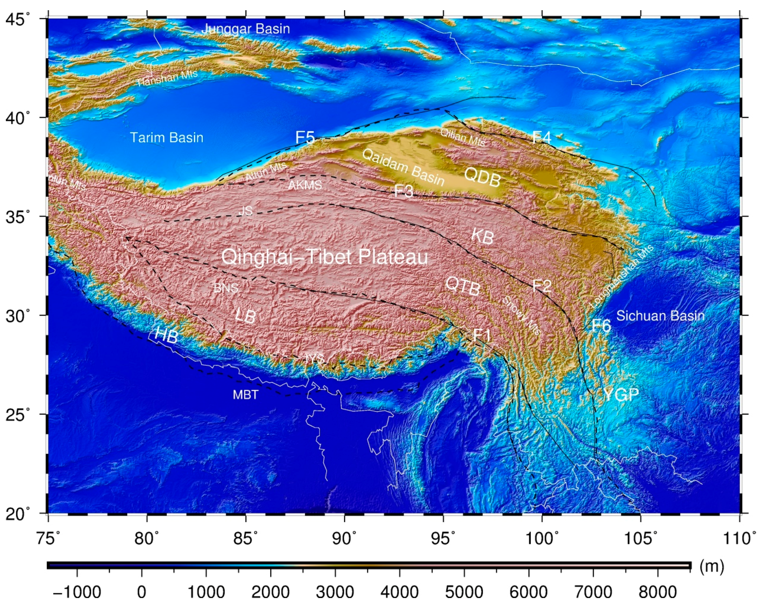
3.1. Study Area and Data Processing

The deepest Moho topography in the world is located beneath Tibet Plateau, which is supposed to be born in the collision of the Indian Plate with the Asian Plate about 57 million years ago [43,44,45]. After the long-term tectonic movements, Tibet, the highest plateau of the Earth, consists of several tectonic blocks, the Himalayan (HB), Lhasa Block (LB), Qiangtang Block (QTB), Kunlun Block (KB) and Qaidam Block (QDB), separated by the sutures, the Indus-Yarlung suture (IYS), Bangong-Nujiang suture (BNS), Jinshajiang suture (JRS) and Anyimaqen-Kunlun-Mutztagh suture (AKMS), respectively (see Figure 1). The tectonic structure of this area is surprisingly complicated and the mechanism of uplift of the central and eastern plateau remains in debate. Argand (1924) proposed that the Indian crust underthrusts most of Tibet, resulting in the double crust thickness [46]. Another possible interpretation is the partially molten middle-lower crust exiting beneath the plateau, forming as a flow channel for mass transfer [47], supported by the low shear velocity zone found in the middle-lower crust beneath Tibet [48]. An accurate Moho model may help figure out the contribution of crust duplexing and crust flow to the formation of the plateau. Therefore, we aimed to study the Moho topography in Tibet using our new approach mentioned previously. Additionally. the area we chose is a little larger than the plateau to reduce the boundary effect during the inversion. Figure 1 shows the topography and primary tectonic elements of study area with the latitude ranging from 20°N to 45°N, and longitude from 75°E to 110°E.

Subsequently, three principal components (${\mathrm{\Gamma }}_{xx}$, ${\mathrm{\Gamma }}_{yy}$ and ${\mathrm{\Gamma }}_{zz}$) of GOCE level-2 calibrated gravity gradients in the Local North-Oriented Reference Frame (LNOF) with the name of EGG_TRF_2_ were employed in this paper [50]. The data span was from November 2009 to August 2012, during which the height of the orbit was quite stable at approximately 260 km. The gravity gradient disturbances ($V_{xx}$, $V_{yy}$ and $V_{rr}$) were achieved, after the normal values of gravity gradients produced by reference ellipsoid (WGS84) were removed from ${\mathrm{\Gamma }}_{xx}$, ${\mathrm{\Gamma }}_{yy}$ and ${\mathrm{\Gamma }}_{zz}$, respectively. Then, $V_{xx}$, $V_{yy}$ and $V_{rr}$ with various heights were reduced on a sphere of $r=6633.4 km$ using the upward or downward continuation method, and the derivatives of the disturbances versus height were derived from the global gravity field model EIGEN6C4 with the largest degree of 280. Then, the $V_{xx}$, $V_{yy}$ and $V_{rr}$ on the sphere were gridded at 10′×10′ by Shepard’s method with the power of 2 and the radium of 20′ based on many experiments, and the results are shown in Figure 2.

From Figure 2, the gravity gradient disturbances range from approximately −1.5 E (1E = 10⁻⁹ s⁻²) to 1.2 E. The signals of $V_{rr}$ are a little stronger than those of $V_{xx}$ and $V_{yy}$. In addition, all the three components are related to the surface topography (Figure 1), and also consistent with the main tectonic blocks. The positive values of $V_{rr}$ are corresponding to areas with high elevation. The max value locates at the Indian-Asian tectonic boundary in the HB, while the negatives outline the three basins, Sichuan Basin, Qaidam Basin and Tarim Basin. The distribution of $V_{xx}$ is almost opposite to that of $V_{rr}$, where the gravity highs are located at basins and gravity lows agree with the high mountains. Moreover, the spatial pattern of $V_{xx}$ seems to be less sensitive along the east-west direction, because the tectonic blocks mainly vary along the north-south direction. In contrast, the spatial pattern of $V_{yy}$ is sensitive along an east-west direction. There is an obvious north-south banded gravity low along the meridian of longitude about 95°. Thus, the spatial patterns of $V_{xx}$, $V_{yy}$ and $V_{rr}$ primarily reflect the mass distributions in north-south, west-east and vertical directions, respectively. The Moho topography of Tibet will then be inverted using these three gravity gradient disturbances.

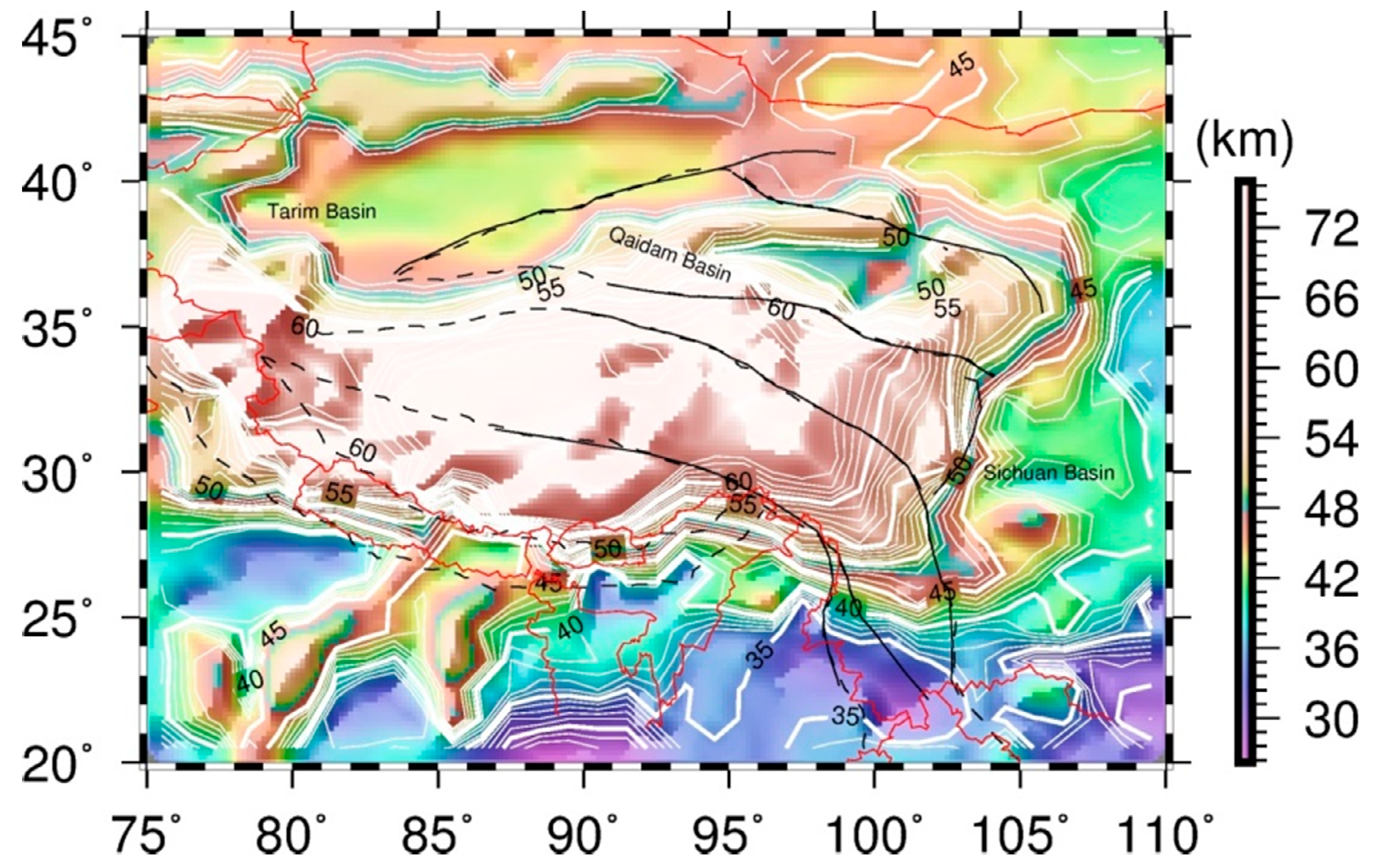
3.2. Moho Topography

Based on the $V_{xx}$, $V_{yy}$ and $V_{rr}$ obtained in the last section, $W$ were inverted using Equation (9) where the $\alpha$ is set as 0.68, 0.70, 0.66, 1.23 for three single component inversions and their joint inversion respectively by the L-curve method. In addition, the results are shown in Figure 3.

In Figure 3, the spatial patterns of $W$ from $V_{xx}$, $V_{yy}$, $V_{rr}$ and their joint inversion are quite similar, and also in good agreement with the primary tectonic structures, which demonstrates that our deduction for $W$ is correct and efficient. The three basins are depicted clearly by gravity lows, and the bordering sutures and major faults are nearly located at gravity high-low transfer zones. On the left of 95°E, there are apparent nearly east-west trending folds, while the folds turn to be almost south-north on the right of 95°E. These are consistent with the crustal south-north shortening and material eastward extrusion under the force of India-Eurasia convergence. Certainly, there are also a few small differences (see Figure 3). The jagged pattern can be observed clearly in the HB and Qilian Mountain from Figure 3b, which further indicates that $W$ from $V_{yy}$ has better resolution along the east-west direction than that from $V_{xx}$ and $V_{yy}$. It also shows that it is necessary to combine different gravity gradient components for determining the Moho topography.

Subsequently, $\delta g_n^{TB}$ was calculated using Earth 2014 [51] with the truncation degree of 180, in which the topography and bathymetric information comes from ETOPO1 and SRTM30_PLUS. $\delta g_n^S$ was computed from the global seismic crustal model CRUST 1.0 [52]. Finally, inserting the estimated $W$, $\delta g_n^{TB}$ and $\delta g_n^S$ into Equation (1), the Moho depths $T$ in Tibet were determined from $V_{xx}$, $V_{yy}$, $V_{rr}$ and their joint inversion, where $\Delta {\rho }_0$= 661.9 kg/m³, $T_0$ = 22.9 km, and $\Delta \rho$ = 448.9 kg/m³ according to the CRUST 1.0. The inverted Moho topography is shown in Figure 4.

As illustrated in Figure 4, the spatial patterns of the MX, MY, MZ and MJ are extremely similar. Overall, the Moho depths in the center and western plateau are deeper than 60 km, which agree with those from [53] and [54]. The Moho topography at the boundary of the plateau is severely steep, such as the HB. It deepens from approximately 40 km in the south to 60 km in the north. The average Moho depth of the HB is approximately 50 km, which is consistent with the results given by [55] and [3]. The Moho depths of the three basins, Qaidam Basin, Tarim Basin and Sichuan Basin, are a little shallower, whose mean values are approximately 50, 42 and 40 km, respectively. These results correspond to those provided by [12] and [2]. In addition, obvious Moho folds can be observed from the shades in Figure 4, whose direction presents a clockwise pattern. In central and west Tibet (on the left of 95°E), the direction of Moho folds is nearly east-west, which is orthogonal to the north-south extrusion force from India-Eurasia convergence. However, the deformation direction of the Moho folds in eastern Tibet (on the right of 95°E) turns to be nearly north-south. The reason may be that the low-density materials in the middle and lower crust of central Tibet are flowing eastward [56,57,58]. This clockwise pattern of Moho folds is also consistent with the GPS velocity field of crustal motion relative to a stable Eurasia (see Figure 4c).

Nevertheless, there are also a few small differences among the MX, MY, MZ and MJ. The deepest Moho is approximately 68.2, 71.1, 69.4 and 68.5 km in the MX, MY, MZ and MJ, whose locations are respective at (78.5°E, 34.5°N), (80.5°E, 35.5°N), (78.5°E, 34.5°N) and (79.5°E, 34.5°N) in the western Kunlun area. Their average results are consistent with the result in [33] of 72 km depth and the result in [3] of (79°E, 35°N).

According to above analysis, the inverted Moho topography is in good agreement with those provided by previous publications, and can also fully reveal the tectonic feature of study area, which verifies the correctness and effectiveness of our method. Moreover, the inverted results by the different gravity gradient disturbances are consistent on the whole, which further improves the credibility of our method.

To verify the regional recognition capability of our method, the Moho topography in Tibet derived from the CRUST 1.0 is shown in Figure 5. Additionally, differences between this study and the CRUST 1.0 are presented in

Table 1. Statistics of Moho depths from various methods and their differences (unit: km), COFF denotes the correlation coefficient (unitless). MAX, MIN, MEAN, STD, and RMS are the maximum, minimum, average, standard deviation and root mean square, respectively. “/” denotes none.

Name	MAX	MIN	MEAN	STD	RMS	COFF
CRUST 1.0	74.81	27.00	47.74	9.91	/	/
MX	68.16	27.07	48.31	9.62	/	/
MY	71.14	30.19	49.48	9.54	/	/
MZ	69.45	27.81	48.89	9.60	/	/
MJ	68.51	26.76	48.83	9.71	/	/
MX-CRUST 1.0	17.63	−17.12	0.57	5.59	5.61	0.84
MY-CRUST 1.0	20.40	−15.39	1.74	5.72	5.98	0.83
MZ-CRUST 1.0	18.46	−15.50	1.15	5.44	5.56	0.85
MJ-CRUST 1.0	19.16	−15.39	1.09	5.54	5.64	0.84

.

Comparing Figure 4 and Figure 5, the spatial patterns of Moho topography between our study and CRUST 1.0 are similar. However, the Moho folds are not apparent in the CRUST 1.0, which indicates that the spatial resolution of our results is better. In Table 1, the MAX from CRUST 1.0 is 74.81 km, which is a little deeper than that of this study. The STD of Moho depths is close to 10 km, denoting violent undulations in this area. The RMS of the differences in Moho depths between CRUST 1.0 and this paper are respectively, 5.61, 5.98, 5.56 and 5.64 km for MX, MY, MZ and MJ, which reasonably correspond to those from [33] and [37]. Besides, the COFF between Moho depths from this study and those from CRUST 1.0 is approximately 0.84, 0.83, 0.85 and 0.84, respectively. According to the comparison, it demonstrates that our method has good large-scale regional recognition capability to invert Moho topography.

To validate the local recognition capability of our method, another model was employed from [59], which provides the discrete crustal thickness in India and Tibet with new constraints using the receiver functions. Crustal thickness is the sum of Moho depth below the sea level and the elevation above the sea level. For comparison, the Moho depths from MJ and the CRUST 1.0 were transferred to crustal thickness by adding the elevations of surface provided by the CRUST 1.0. Figure 6 shows the crustal thickness from Singh et al. (2017) [59], CRUST 1.0 and MJ. The receiver functions are regarded as the most powerful tool for revealing the crustal thickness, and the results from [59] are considered to be the most reliable model. Hence, we compared the MJ and CRUST 1.0 with [59], respectively (see Figure 7).

Table 2. Statistics of crustal thickness for the three models and their differences (unit: km).

Name	MAX	MIN	MEAN	STD	RMS	COFF (Unitless)
Singh et al. (2017)	86.82	31.60	60.32	11.92	/	/
MJ	71.52	33.05	59.89	11.16	/	/
CRUST 1.0	75.04	35.59	60.01	11.03	/	/
MJ-Singh et al. (2017)	20.44	−21.15	−0.44	5.88	5.90	0.87
CRUST 1.0- Singh et al. (2017)	14.98	−15.43	−0.32	5.33	5.34	0.89

lists the statistics of crustal thickness for the three models and their differences.

From Figure 6 and Table 2, the range of crustal thickness provided by Singh et al. (2017) is from 31.60 to 86.82 km, which is larger than that of MJ. The STD of Singh et al. (2017) is also bigger than that from MJ. It demonstrates that the local recognition capability of the seismic method for detecting Moho topography is better than that of the gravity method, if the seismic stations are dense. The reason is that gravity data primarily reflects the superposition of all materials within the Earth interior and its advantage is to investigate large-scale regional lateral mass distribution, rather than that of one point.

As illustrated in Figure 7 and Table 2, the RMS of the differences between CRUST 1.0 and Singh et al. (2017) [59] is 5.34 km and the COFF is 0.89, which indicates that the Moho topography of the CRUST 1.0 in Tibet may need to be improved further using denser data. The RMS and COFF between MJ and Singh et al. (2017) [59] are respectively 5.90 km and 0.87. It shows that the local recognition capability of MJ is approximately the same as that of the CRUST 1.0.

In summary, the regional spatial resolution of the inverted Moho topography from gravity gradient disturbances using our new method is better than that of CRUST 1.0, while the local recognition capability of the two models is almost same. Thus, our models can provide more details about the tectonic structure, such as the Moho folds.

4. Discussion

In the VMM isostasy theory, the density anomalies below the Moho have been ignored, while those of the consolidated crystalline crust should be considered. However, in this study, the density anomalies of the consolidated crystalline crust are ignored as well, whose reason is that the existing crustal density models in Tibet, such as CRUST 1.0, are not accurate due to the sparse seismic station coverage especially in center and western Tibet [2,3,49]. It may affect our results, where higher density (larger than 2.67 g/cm³) results in shallower Moho depths during the inversion, and lower density (less than 2.67 g/cm³) can cause deeper estimated results. Figure 7b is the map of the differences between MJ and that from [59]. The largest negatives appear in India near the north coast of the Bay of Bengal, which may be explained by the high density of the oceanic crust. In addition, the largest positives are located in the YGP, indicating low density in the crust which is supported by previous research [60]. Therefore, the primary reason for the differences between our Moho model from gravity and the seismic Moho model may be the poor crustal density model.

Further, the velocity model of shear wave from [61] was employed to analyze the differences between MJ and that of the CRUST1.0 (see Figure 8). Low shear wave velocity zone can be found in the middle and lower crust beneath Tibet, showing the high temperature [62] and probably partial melting of the rocks existing in this area [48]. As the rocks are heated, their density decreases through thermal expansion [63], which leads to negative gravity anomalies. Thus, the low velocity zone of shear wave should locate at where the Moho in MJ is deeper than that in CRUST1.0, and the high velocity zone should locate at where the Moho in MJ is shallower than that in CRUST1.0.

In Figure 8a, the Moho depths in MJ are remarkably deeper at the west of LB along BNS and KB along JS, beneath Qilian Mountain and in the east of YGP, where the corresponding low velocity zones can be found in Figure 8b. Similarly, the Moho depths are shallower during MJ and the corresponding shear wave velocity is high underneath the three basins (Sichuan Basin, Qaidam Basin, Tarim Basin). However, in center Tibet, the Moho depths in MJ and shear wave velocity are shallower and low respectively, which may be explained as the high velocity of shear wave in the uppermost mantle of this area.

In addition, the differences among $W$ from single gradient disturbances $V_{xx}$, $V_{yy}$ and $V_{rr}$ are remarkable (see Figure 3), because of their inherent variances of sensitivities to different directions. Thus, in theory the inverted Moho depths from $V_{xx}$, $V_{yy}$ and $V_{rr}$ should be different. Nevertheless, the obtained Moho topography from them and their joint inversion are very similar (see Figure 4). The main reason may be that the influence of topography/bathymetry on the Moho depths in Equation (1) is much larger than the others. The effect of $\delta g_n^{TB}$ on the Moho depths varies from –6.67 to 35.38 km with the STD of 10.31 km, while the influence caused by $W$ varies from –16.08 to 14.04 km with the STD of 4.18 km. Thus, the differences among $W$ from $V_{xx}$, $V_{yy}$ and $V_{rr}$ are probably hidden by the $\delta g_n^{TB}$.

5. Conclusions

Based on the solution of the VMM problem of isostasy, we developed a new approach to recover Moho topography by using the three principle components of gravity gradients derived from GOCE. Four Moho models (MX, MY, MZ and MJ) of Tibet were inverted by our method, whose spatial patterns were extremely similar. The inverted Moho topographies were consistent with those from previous studies and can reflect the primary tectonic feature as well. The deepest Moho depth is approximately 70 km, located at the western Kunlun region. The apparent Moho folds can be detected, the direction of which presents a clockwise pattern. There results verify the correctness of our method.

The comparison between our inverted Moho models and that of CRUST 1.0 was conducted. The COFF and RMS of the differences between these two models were in agreement with those provided by previous studies. Yet, our model can identify the Moho folds and has better spatial resolution. Further, the local recognition capability of our method was verified by comparing our Moho model with that of Singh et al. (2017) [59], which shows that the local recognition between our model and CRUST 1.0 is similar.

Lastly, the possible reasons for the differences between our Moho model from gravity and the seismic Moho model were analyzed. By comparing the Moho depth differences with shear wave velocity, it confirmed that the primary reason is the poor crustal density model in Tibet. Therefore, at present the uncertainty of crustal density structure is an inhibited factor to determine refined Moho topography using gravity data as the implementation of gravity satellite plans, which needs to be improved in the future.

References

1. Gao, R.; Xiong, X.; Li, Q.; Lu, Z. The Moho depth of Qinghai-Tibet Plateau revealed by seismic detection. Acta Geosci. Sin. 2009, 30, 761–773. [Google Scholar]
2. Shin, Y.H.; Shum, C.K.; Braitenberg, C.; Lee, S.M.; Na, S.; Choi, K.S.; Hsu, H.; Park, Y.; Lim, M. Moho topography, ranges and folds of Tibet by analysis of global gravity models and Goce data. Sci. Rep. 2015, 5, 1–7. [Google Scholar] [CrossRef] [PubMed]
3. Xu, C.; Liu, Z.W.; Luo, Z.C.; Wu, Y.H.; Wang, H.H. Moho topography of the Tibetan Plateau using multi-scale gravity analysis and its tectonic implications. J. Asian Earth Sci. 2017, 138, 378–386. [Google Scholar] [CrossRef]
4. Tapponnier, P.; Peltzer, G.; Le Dain, A.Y.; Armijo, R. Propagating extrusion tectonics in Asia: New insights from simple experiments with plasticine. Geology 1982, 10, 611–616. [Google Scholar] [CrossRef]
5. Gao, R.; Chen, C.; Lu, Z.; Brown, L.D.; Xiong, X.; Li, W.; Deng, G. New constraints on crustal structure and Moho topography in Central Tibet revealed by SinoProbe deep seismic reflection profiling. Tectonophysics 2013, 606, 160–170. [Google Scholar] [CrossRef] [Green Version]
6. Tseng, J.; Kan, Y. Deep sub-basement reflections in the western part of Chai-da-mu Basin. Chin. J. Sin. 1961, 10, 120–125. [Google Scholar]
7. Zhao, W.; Nelson, K.D.; Che, J.; Quo, J.; Lu, D.; Wu, C.; Liu, X. Deep seismic reflection evidence for continental underthrusting beneath southern Tibet. Nature 1993, 366, 557–559. [Google Scholar] [CrossRef]
8. Kao, H.; Gao, R.; Rau, R.; Shi, D.; Chen, R.; Guan, Y.; Wu, F.T. Seismic image of the Tarim basin and its collision with Tibet. Geology 2001, 29, 575–578. [Google Scholar] [CrossRef]
9. Kind, R.; Yuan, X.; Saul, J.; Nelson, D.; Sobolev, S.V.; Mechie, J.; Zhao, W.; Kosarev, G.; Ni, J.; Achauer, U.; et al. Seismic images of crust and upper mantle beneath Tibet: Evidence for Eurasion plate subduction. Science 2002, 298, 1219–1221. [Google Scholar] [CrossRef]
10. Xu, Y.; Liu, F.; Liu, J.; Chen, H. Crust and upper mantle structure beneath western China from P wave travel time tomography. J. Geophys. Res. 2002, 107, 2220. [Google Scholar] [CrossRef]
11. Zhang, Z.; Klemperer, S.L. West-east variation in crustal thickness in northern Lhasa block, central Tibet, from deep seismic sounding data. J. Geophys. Res. 2005, 110, B09403. [Google Scholar] [CrossRef]
12. Zhao, J.; Mooney, W.D.; Zhang, X.; Li, Z.; Jin, Z.; Okaya, N. Crustal structure across the Altyn Tagh Range at the northern margin of the Tibetan Plateau and tectonic implications. Earth Planet. Sci. Lett. 2006, 241, 804–814. [Google Scholar] [CrossRef]
13. Xu, L.; Rondenay, S.; van der Hist, R.D. Structure of the crust beneath the southeastern Tibetan Plateau from teleseismic receiver functions. Phys. Earth Planet. Int. 2007, 165, 176–193. [Google Scholar] [CrossRef]
14. Zhang, X.; Sun, R.; Teng, J. Study on crustal, lithospheric and asthenospheric thickness beneath the Qinghai-Tibet Plateau and its adjacent areas. Chin. Sci. Bull. 2007, 52, 797–804. [Google Scholar] [CrossRef]
15. Lou, H.; Wang, C.; Lü, Z.; Yao, Z.; Dai, S.; You, H. Deep tectonic setting of the 2008 Wenchuan Ms8.0 earthquake in southwestern China. Sci. China Ser. D Earth Sci. 2009, 52, 166–179. [Google Scholar] [CrossRef]
16. Lu, Z.; Gao, R.; Li, Q.; He, R.; Kuang, C.; Hou, H.; Xiong, X.; Guan, Y.; Wang, H. Test of deep seismic reflection profiling across central uplift of Qiangtang terrane in Tibetan Plateau. J. Earth Sci. 2009, 20, 438–447. [Google Scholar] [CrossRef]
17. Yang, H.; Hu, J.; Li, G.; Zhao, H.; Wen, L. Analysis of the crustal thickness and Poisson’s ratio in eastern Tibet from teleseismic receiver functions. Geophys. J. Int. 2011, 186, 1380–1388. [Google Scholar] [CrossRef]
18. Obrebski, M.; Allen, R.M.; Zhang, F.; Pan, J.; Wu, Q.; Hung, S. Shear wave tomography of China using joint inversion of body and surface wave constraints. J. Geophys. Res. 2012, 117, B01311. [Google Scholar] [CrossRef]
19. Xu, X.; Ding, Z.; Shi, D.; Li, X. Receiver function analysis of crustal structure beneath the eastern Tibetan plateau. J. Asian Earth Sci. 2013, 73, 121–127. [Google Scholar] [CrossRef]
20. Tian, X.; Liu, Z.; Si, S.; Zhang, Z. The crustal thickness of NE Tibet and its implication for crustal shortening. Tectonophysics 2014, 634, 198–207. [Google Scholar] [CrossRef]
21. Koulakov, I.; Maksotova, G.; Mukhopadhyay, S.; Raoof, J.; Kayal, J.R.; Jakovlev, A.; Vasilevsky, A. Variations of the crustal thickness in Nepal Himalayas based on tomographic inversion of regional earthquake data. Solid Earth 2015, 6, 207–216. [Google Scholar] [CrossRef] [Green Version]
22. Zheng, H.; Li, T.; Gao, R. The progress of seismic tomography research in the Tibetan Plateau. Geophys. Geochem. Explor. 2011, 35, 160–164. [Google Scholar]
23. Tapley, B.D.; Bettadpur, M.; Watkins, M.; Reigber, C. The gravity recovery and climate experiment: Mission overview and early results. Geophys. Res. Lett. 2004, 31, L09607. [Google Scholar] [CrossRef]
24. Zhou, H.; Luo, Z.; Zhou, Z.; Li, Q.; Zhong, B.; Lu, B.; Hsu, H. Impact of different kinematic empirical parameters processing strategies on temporal gravity field model determination. J. Geophys. Res. Solid Earth 2018, 123, 10252–10276. [Google Scholar] [CrossRef]
25. Rummel, R.; Balmino, G.; Johannessen, J.; Visser, P.; Woodworth, P. Dedicated gravity field missions—Principle and aims. J. Geodyn. 2002, 33, 3–20. [Google Scholar] [CrossRef]
26. Vening Meinesz, F.A. Une nouvelle méthode pour la réduction isostatique régionale de Í intensité de la pesanteur. Bull. Geod. 1931, 29, 33–51. [Google Scholar] [CrossRef]
27. Parker, R.L. The rapid calculation of potential anomalies. Geophys. J. R. Astron. Soc. 1972, 31, 447–455. [Google Scholar] [CrossRef]
28. Shin, Y.H.; Xu, H.Z.; Braitenberg, C.; Fang, J.; Wang, Y. Moho undulations beneath Tibet from GRACE-integrated gravity data. Geophys. J. Int. 2007, 170, 971–985. [Google Scholar] [CrossRef] [Green Version]
29. Shin, Y.H.; Shum, C.K.; Braiternberg, C.; Lee, S.M.; Xu, H.; Choi, K.S.; Baek, J.H.; Park, J.U. Three-dimensional fold structure of the Tibetan Moho from Grace gravity data. Geophys. Res. Lett. 2009, 36, L01302. [Google Scholar] [CrossRef]
30. Moritz, H. (Ed.) The Figure of the Earth; Wichmann: Karlsruhe, Germany, 1990. [Google Scholar]
31. Sjöberg, L.E. Solving Vening Meinesz-Moritz inverse problem in isostasy. Geophys. J. Int. 2009, 179, 1527–1536. [Google Scholar] [CrossRef] [Green Version]
32. Sjöberg, L.E.; Bagherbandi, M. A method of estimating the Moho density contrast with a tentative application by EGM08 and CRUST2.0. Acta Geophys. 2011, 59, 502–525. [Google Scholar] [CrossRef]
33. Oldenburg, D.W. The inversion and interpretation of gravity anomalies. Geophysics 1974, 39, 526–536. [Google Scholar] [CrossRef]
34. Bagherbandi, M. A comparison of three gravity inversion methods for crustal thickness modelling in Tibet plateau. J. Asian Earth Sci. 2012, 43, 89–97. [Google Scholar] [CrossRef]
35. Tenzer, R.; Chen, W. Expressions for the global gravimetric Moho modeling in spectral domain. Pure Appl. Geophys. 2014, 171, 1877–1896. [Google Scholar] [CrossRef]
36. Chen, W.; Tenzer, R. Moho modeling in spatial domain: A case study under Tibet. Adv. Space Res. 2017, 59, 2855–2869. [Google Scholar] [CrossRef]
37. Eshagh, M.; Hussain, M.; Tenzer, R.; Romeshkani, M. Moho density constrast in central Eurasia from GOCE gravity gradients. Remote Sens. 2016, 8, 418. [Google Scholar] [CrossRef]
38. Eshagh, M.; Hussain, M. An approach to Moho discontinuity recovery from on-orbit GOCE data with application over Indo-Pak region. Tectonophysics 2016, 690, 253–262. [Google Scholar] [CrossRef]
39. Eshagh, M.; Ebadi, S.; Tenzer, R. Isostatic GOCE Moho model for Iran. J. Asian Earth Sci. 2017, 138, 12–24. [Google Scholar] [CrossRef]
40. Wu, Y.; Zhou, H.; Zhong, B.; Luo, Z. Regional gravity field recovery using the GOCE gravity gradient tensor and heterogeneous gravimetry and altimetry data. J. Geophys. Res. Solid Earth 2017, 122, 6928–6952. [Google Scholar] [CrossRef]
41. Tikhonov, A.N. Solution of incorrectly formulated problems and regularization method. Sov. Math. Doki. 1963, 4, 1035–1038. [Google Scholar]
42. Hansen, P.C.; O’Leary, D.P. The use of the L-curve in the regularization of discrete ill-posed problems. Siam J. Sci. Comput. 1993, 14, 1487–1503. [Google Scholar] [CrossRef]
43. Leech, M.L.; Singh, S.; Jain, A.; Klemperer, S.L.; Manickavasagam, R. The onset of India-Asia continental collision: Early, steep subduction required by the timing of UHP metamorphism in the western Himalaya. Earth Planet. Sci. Lett. 2005, 234, 83–97. [Google Scholar] [CrossRef]
44. Li, Q.; Gao, R.; Lu, Z.; Guan, Y.; Zhang, J.; Li, P.; Karplus, M. The thickness and structural characteristics of the crust across Tibetan plateau from active-sources seismic profiles. Earthq. Sci. 2009, 22, 21–31. [Google Scholar] [CrossRef] [Green Version]
45. Gao, R.; Lu, Z.; Klemperer, S.L.; Wang, H.; Dong, S.; Li, W.; Li, H. Crustal-scale duplexing beneath the Yarlung Zangbo suture in the western Himalaya. Nat. Geosci. 2016, 9, 555. [Google Scholar] [CrossRef]
46. Argand, E. La Tectonique de l’Asie. In Proceedings of the 13th International Geological Congress, Brussels, Belgium, August 1922; pp. 171–372. [Google Scholar]
47. Nelson, K.D. Partially molten middle crust beneath southern Tibet; synthesis of Project INDEPTH result. Science 1996, 274, 1684–1688. [Google Scholar] [CrossRef]
48. Yang, Y.; Ritzwoller, M.H.; Zheng, Y.; Shen, W.; Levshin, A.L.; Xie, Z. A synoptic view of the distribution and connectivity of the mid-crustal low velocity zone beneath Tibet. J. Geophys. Res. 2012, 117. [Google Scholar] [CrossRef]
49. Xu, C.; Luo, Z.; Sun, R.; Zhou, H.; Wu, Y. Multilayer densities using a wavelet-based gravity method and their tectonic implications beneath the Tibetan Plateau. Geophys. J. Int. 2018, 213, 2085–2095. [Google Scholar] [CrossRef]
50. Gruber, T.; Rummel, R.; Abrikosov, O.; van Hees, R. GOCE level 2 Product Data Handbook. GO-MA-HPF-GS-0110, Issue 4.3 2010. Available online: https://earth.esa.int/c/document_library/get_file?folderId=14168&name=DLFE-591.pdf (accessed on 28 June 2019).
51. Hirt, C.; Rexer, M. Earth2014: 1 arc-min shape, topography, bedrock and ice-sheet models – Available as gridded data and degree—10,800 spherical harmonics. Int. J. Appl. Earth Obs. Geoinf. 2015, 39, 103–112. [Google Scholar] [CrossRef]
52. Laske, G.; Masters, G.; Ma, Z.; Pasyanos, M. Update on CRUST1.0—A 1-degree global model of Earth’s crust. EGU Gen. Assem. Conf. Abstr. 2013, 15, 2658. [Google Scholar]
53. Yin, Z.; Teng, J.; Liu, H. The 2-D crustal structure study in the Yadong-Damxung region of the Xizang Plateau. Bull. Chin. Acad. Geol. Sci. 1990, 21, 239–245. [Google Scholar]
54. Li, H.; Xu, X.; Jiang, M. Deep dynamical processes in the central-southern Qinghai-Tibet Plateau—Receiver functions and travel-time residuals analysis of north Hi-Climb. Sci. China Ser. D Earth Sci. 2008, 51, 1297–1305. [Google Scholar] [CrossRef]
55. Hirn, A.; Nercessian, A.; Sapin, M.; Jobert, G.; Xu, Z.; Gao, E.; Lu, D.; Teng, J. Lhasa block and bordering sutures-a continuation of a 500-km Moho traverse through Tibet. Nature 1984, 307, 25–27. [Google Scholar] [CrossRef]
56. Royden, L.H.; Burchfiel, B.C.; King, R.W.; Wang, E.; Chen, Z.; Shen, F.; Liu, Y. Surface deformation and lower crustal flow in eastern Tibet. Science 1997, 276, 788–790. [Google Scholar] [CrossRef] [PubMed]
57. Royden, L.H.; Burchfiel, B.C.; van der Hilst, R.D. The geological evolution of the Tibetan Plateau. Science 2008, 321, 1054–1058. [Google Scholar] [CrossRef] [PubMed]
58. Clark, M.K.; Royden, L.H. Topographic ooze: Building the eastern margin of Tibet by lower crustal flow. Geology 2000, 28, 703–706. [Google Scholar] [CrossRef]
59. Singh, A.; Ravi Kumar, M.; Mohanty, D.D.; Singh, C.; Biswas, R.; Srinagesh, D. Crustal structure beneath India and Tibet: New constraints from inversion of receiver functions. J. Geophys. Res. Solid Earth 2017, 122, 7839–7859. [Google Scholar] [CrossRef]
60. Deng, Y.; Zhang, Z.; Basal, J.; Fan, W. 3-D density structure under South China constrained by seismic velocity and gravity data. Tectonophysics 2014, 627, 159–170. [Google Scholar] [CrossRef]
61. Shen, W.; Ritzwoller, M.H.; Kang, D.; Kim, Y.; Ning, J.; Lin, F.C.; Wang, W.; Zheng, Y.; Zhou, L. A seismic reference model for the crust and uppermost mantle beneath China from surface wave dispersion. Geophys. J. Int. 2016, 206, 954–979. [Google Scholar] [CrossRef] [Green Version]
62. Kern, H.; Popp, T.; Gorbatsevich, F.; Zharikov, A.; Lobanov, K.V.; Smirnov, Y.P. Pressure and temperature dependence of VP and VS in rocks from the superdeep well and from surface analogues at Kola and the nature of velocity anisotropy. Tectonophysics 2001, 338, 113–134. [Google Scholar] [CrossRef]
63. Currie, C.A. The deep roots of the Rocky Mountains: Geophysical studies of western Canada. J. Stud. Sci. Technol. 2016, 9, 35–41. [Google Scholar] [CrossRef]
Figure 1. The topography and primary tectonic elements of study area (modified from [49]). The black dashed lines, black solid lines and white lines are bordering sutures, major faults and national borders, respectively. Key to symbols: HB, Himalayan Block; LB, Lhasa Block; QTB, Qiangtang Block; KB, Kunlun Block; QDB, Qaidam Block; YGP, Yunnan-Guizhou Plateau; MBT, Main Boundary Thrust; IYS, Indus-Yarlung suture; BNS, Bangong-Nujiang suture; JS, Jinshajiang suture; AKMS, Anyimaqen-Kunlun-Mutztagh suture; F1, Jiali Fault; F2, Manyi Yushu Xianshuihe Fault; F3, Kunlun Fault; F4, Haiyuan Fault; F5, Altyn Tagh Fault; F6, Longmenshan Fault.
Remotesensing 11 01567 g001
Figure 2. Gravity gradient disturbances in Tibet after reduction and gridding: (a) V x x , (b) V y y , (c) V r r . The directions of coordinate axis x , y and r are north, west and vertical upward, respectively. The major tectonic elements (see Figure 1) are overlain on the map for assistant analysis.
Remotesensing 11 01567 g002
Figure 3. Estimated values of the parameter W from (a) V x x ; (b) V y y ; (c) V r r ; (d) joint inversion of V x x , V y y and V r r . The major tectonic elements (see Figure 1) are overlain on the map for assist analysis.
Remotesensing 11 01567 g003
Figure 4. (ad) Inverted Moho depths (MX, MY, MZ and MJ) of Tibet derived from V x x , V y y , V r r and their joint inversion, respectively. Black vectors in (c) are the Global Positioning System (GPS) velocity field of crustal motion relative to the stable Eurasia. The major tectonic elements (see Figure 1) are overlain on the map for assist analysis. The red lines denote the national borders.
Remotesensing 11 01567 g004
Figure 5. Moho depths provided by the CRUST 1.0. The major tectonic elements (see Figure 1) are overlain on the map for assist analysis. The red lines are the national borders.
Remotesensing 11 01567 g005
Figure 6. Crustal thickness from (a) Singh et al. (2017) [59], (b) CRUST1.0, (c) MJ.
Remotesensing 11 01567 g006
Figure 7. (a) Differences of crustal thickness between CRUST1.0 and Singh et al. (2017) [59]; (b) differences of crustal thickness between MJ and Singh et al. (2017) [59].
Remotesensing 11 01567 g007
Figure 8. (a) Moho depth differences between MJ and CRUST 1.0; (b) shear wave velocity at the depth of 30 km.
Remotesensing 11 01567 g008