Assessment of the Dual Polarimetric Sentinel-1A Data for Forest Fuel Moisture Content Estimation
by
 ,
,
Long Wang
1, 
Xingwen Quan
1,*,
Binbin He
1,2,
Marta Yebra
3,4,
Minfeng Xing
1 and
Xiangzhuo Liu
1 1
School of Resources and Environment, University of Electronic Science and Technology of China, Chengdu 611731, China
2
Center for Information Geoscience, University of Electronic Science and Technology of China, Chengdu 611731, China
3
Fenner School of Environment and Society, The Australian National University, Canberra, ACT 2601, Australia
4
Bushfire & Natural Hazards Cooperative Research Centre, Melbourne, VIC 3002, Australia
*
Author to whom correspondence should be addressed.
Remote Sens. 2019, 11(13), 1568; https://0-doi-org.brum.beds.ac.uk/10.3390/rs11131568
Submission received: 21 May 2019
/
Revised: 27 June 2019
/
Accepted: 29 June 2019
/
Published: 2 July 2019
(This article belongs to the Special Issue Remote Sensing and Image Processing for Fire Science and Management)
Abstract
:Fuel moisture content (FMC) is a crucial variable affecting fuel ignition and rate of fire spread. Much work so far has focused on the usage of remote sensing data from multiple sensors to derive FMC; however, little attention has been devoted to the usage of the C-band Sentinel-1A data. In this study, we aimed to test the performance of C-band Sentinel-1A data for multi-temporal retrieval of forest FMC by coupling the bare soil backscatter linear model with the vegetation backscatter water cloud model (WCM). This coupled model that linked the observed backscatter directly to FMC, was firstly calibrated using field FMC measurements and corresponding synthetic aperture radar (SAR) backscatters (VV and VH), and then a look-up table (LUT) comprising of the modelled VH backscatter and FMC was built by running the calibrated model forwardly. The absolute difference (MAEr) of modelled and observed VH backscatters was selected as the cost function to search the optimal FMC from the LUT. The performance of the presented methodology was verified using the three-fold cross-validation method by dividing the whole samples into equal three parts. Two parts were used for the model calibration and the other one for the validation, and this was repeated three times. The results showed that the estimated and measured forest FMC were consistent across the three validation samples, with the root mean square error (RMSE) of 19.53% (Sample 1), 12.64% (Sample 2) and 15.45% (Sample 3). To further test the performance of the C-band Sentinel-1A data for forest FMC estimation, our results were compared to those obtained using the optical Landsat 8 Operational Land Imager (OLI) data and the empirical partial least squares regression (PLSR) method. The latter resulted in higher RMSE between estimated and measured forest FMC with 20.11% (Sample 1), 26.21% (Sample 2) and 26.73% (Sample 3) than the presented Sentinel-1A data-based method. Hence, this study demonstrated that the good capability of C-band Sentinel-1A data for forest FMC retrieval, opening the possibility of developing a new operational SAR data-based methodology for forest FMC estimation.
1. Introduction
Fuel moisture content (FMC) is defined as the proportion of water content over dry mass, which is a vital variable for evaluating wildfire risk since it is directly correlated to the probability of fuel ignition, and the rate and direction of wildfire spread [1]. In this content, spatially and temporally accurate mapping FMC dynamics at the landscape scale is paramount to wildfire risk assessment. To date, remote sensing techniques, providing high spatial and temporal resolution earth observation at local to global scale, are the unique way to that end [2,3].
Studies estimating FMC from remote sensing data have mainly concentrated on utilizing optical remote sensing data [3]. The first studies were conducted in the 1980s and the 1990s for herbaceous species based on the positive relationships between FMC and AVHRR-derived normalized difference vegetation index (NDVI) [4,5]. Since the launch of Terra and Aqua satellites by NASA in 1999 and 2002, the moderate resolution imaging spectroradiometer (MODIS) has attracted more attention to monitor this variable [6,7,8,9]. With the development of optical sensor technology, the medium spatial resolution sensors, represented by thematic mapper (TM, Landsat 4, 5), enhanced thematic mapper (ETM+, Landsat 7) and operational land imager (OLI, Landsat 8) have also been wildly applied to estimate FMC [10,11]. Strong correlations between grasslands FMC and optical remote sensing data have been reported in previous research [12,13,14,15,16]. However, the weaker correlations over shrublands and forest have made the estimation of FMC for these areas challenging. Bowyer et al. [17] theoretically demonstrated that, on the basis of optical remote sensing data, a greater accuracy level is expected when estimating FMC over grasslands than shrublands and forests, due to the fact that the latter land cover suffers from greater confounding influences from variables such as leaf area index (LAI) and fraction of vegetation cover. In addition, the weather conditions (such as cloudy coverage) largely limit the application of optical remote sensing for FMC retrieval because of the limited penetration capacity of the optical signal. Alternatively, microwave remote sensing provides a new opportunity for FMC estimation due to its high sensitivity to surface moisture [18,19,20], as well as its unique capacity to work in cloudy areas.
Recently, active microwave remote sensing technique, represented by the polarimetric synthetic aperture radar (SAR), has attracted much attention for surface variables estimation [21,22,23,24,25]. Satellites equipped with a SAR sensor include L-band ALOS-2, C-band Radarsat-1/2 and Sentinel-1A/B, and X-band TerraSAR-X, TanDEM-X, TecSAR, RISAT-1/2, and SeoSAR [18,26,27,28,29,30]. L-band microwave response results from an interaction of the electromagnetic radiation with the canopy-soil and the backscatter directly from the soil while C-band and X-band microwave interact more with the upper vegetation canopy [31]. Consequently, C-band and X-band radars are considered more suitable for retrieving vegetation canopy properties. Among the C-band and X-band SAR existing datasets, the global time-series dual polarimetric C-band Sentinel-1 A/B data has been freely available since October 2014 and provides a favorable opportunity for long-term monitoring of surface variables. However, to date and to our knowledge, C-band Sentinel-1 A/B data has not been yet used for FMC estimation.
The estimation of surface variables from active microwave remote sensing data is still challenged since distinguishing between backscatters from vegetation and bare soil is difficult [21,23,25]. Over the past few decades, researchers have proposed several bare soil and vegetation backscatter models to depict these backscatters from these two aspects. For bare soil, the bare soil backscatter model can be classified into: (i) Empirical models, such as the linear model [32,33,34], Oh model [35,36,37,38], and the Dubois model [39,40]; (ii) the semi-empirical models, such as the Shi model [41,42] and the Baghdadi model [43]; and (iii) theoretical models, such as the integral equation model (IEM) and advanced IEM [44,45,46]. These models have been successfully applied to estimate the backscatter of bare soil in the process of surface parameters retrieval, such as soil moisture [21,22,23,47,48] and leaf area index [32,49]. On the other hand, vegetation backscatter models generally include the ratio method [50,51,52], the water cloud model (WCM) [53], the Roo model [54], the Michigan microwave canopy scattering model [55,56,57], the Saatchi model [58,59], and the Tor Vergata model [60,61]. Among these bare soil and vegetation backscatter models, the bare soil backscatter linear model and vegetation backscatter WCM have often coupled for surface variables estimation due to their effectiveness and conciseness for modeling the surface backscatters [31].
This study aims to assess the performance of C-band Sentinel-1A data for forest FMC estimation. The overarching objective is to contribute to the development of an operational system that can assist in wildfire risk early prescription, suppression and response, as well as improved awareness of wildfire risk to life and property. To adequately verify the methodology presented in this study, the estimated results of forest FMC were, on one hand, compared with these obtained using the optical Landsat 8 OLI data and empirical partial least squares regression (PLSR) method, and on the other hand were validated through the field forest FMC measurements taken in Texas, USA.
2. Methodology
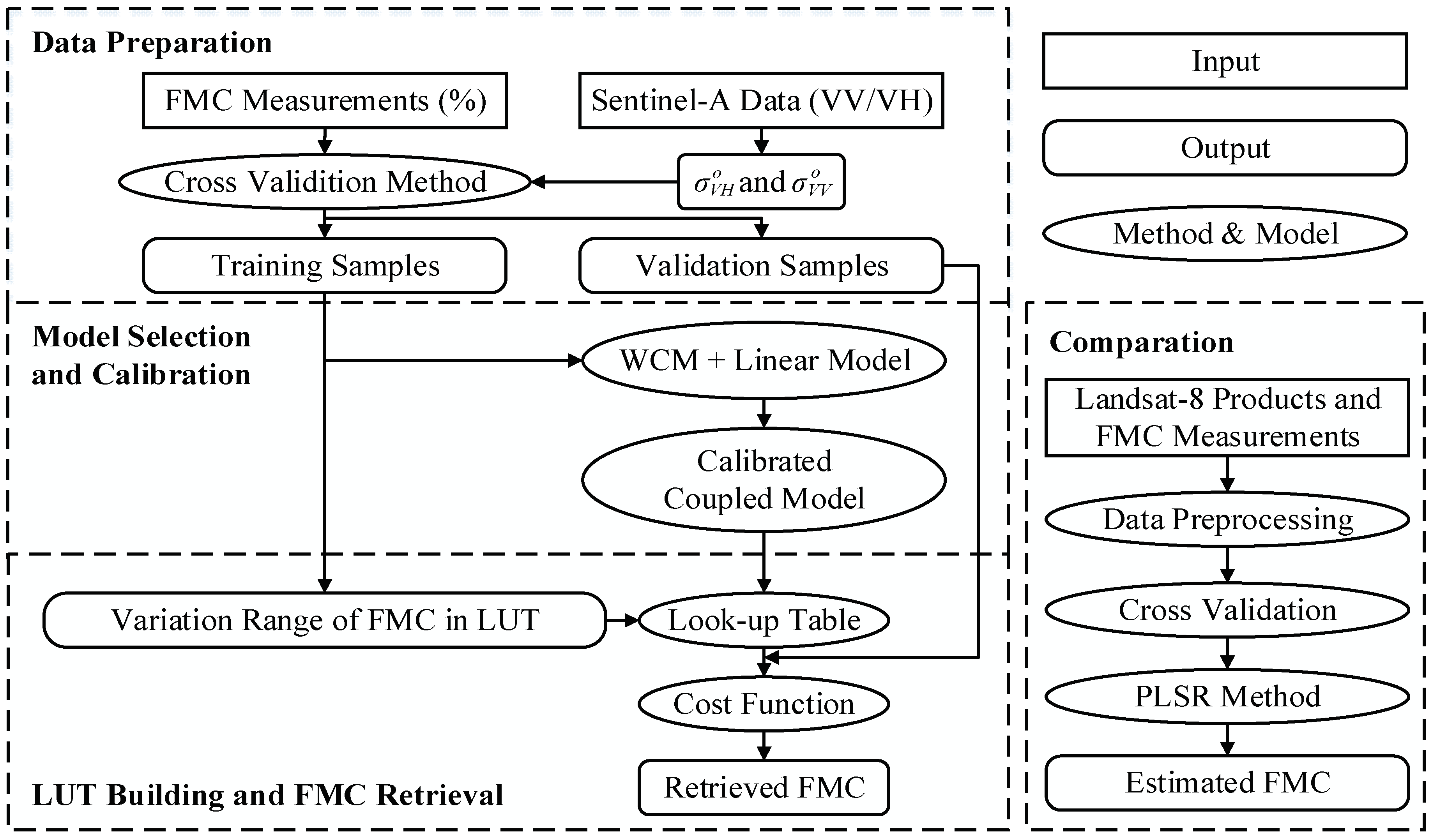
In this study, the empirical bare soil backscatter linear model and the semi-empirical vegetation backscatter WCM were coupled to link the observed backscatter from the dual-polarimetric Sentinel-1A data directly to forest FMC. The performance of the presented method was adequately verified using the three-fold cross-validation method. In addition, to further test the performance of the presented Sentinel-1A data-based method for forest FMC estimation, our results were compared to those obtained using the Landsat 8 OLI data and the PLSR method. A flowchart of the presented method for forest FMC estimation from dual polarimetric Sentinel-1A data is given in Figure 1.
2.1. Data
2.1.1. Field Forest FMC Data
In this study, the field forest FMC measurements used for the calibration and validation of the presented method were downloaded from the National Fuel Moisture Database (NFMD), which is a web-based query system that enables users to view time-series of measured FMC information in USA (https://www.wfas.net/nfmd/public). This system utilizes a database that is routinely updated by fuels specialists who monitor, sample and calculate FMC from 2006 to date.
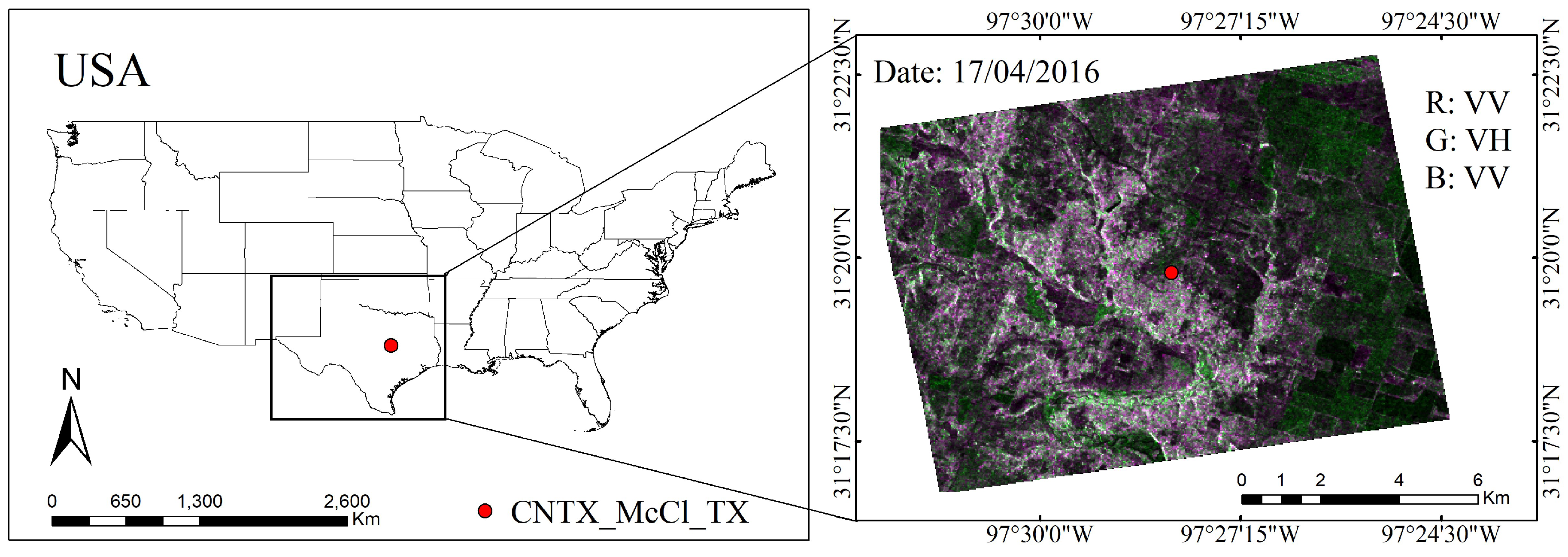
Since the Sentinel-1A data in the USA was only available after 2016, and to reduce the effect of local radar incidence angle, only the FMC measurements sampled in CNTX_McCl_TX site (31°19’48’’N, 97°28’12’’W, with 21 measurements taken in Texas, shown in Figure 2) were selected to verify the performance of the methodology presented in this study. The selected site has a greater number of forest FMC measurements and available Sentinel-1A images compared with the other sites included in this database. The FMC data were measured every 30 days from May 2016 to January, 2018 (see Appendix A, Table A1). The vegetation species in this site are heterogeneous and mixed with Bluestem, Juniper, Redberry and Oak. The sampling area is about 5 acres, and the sampling plots were relatively homogeneous distributed in terms of species composition, canopy cover, aspect, and slope steepness. About 5 to 15 samples per species within the site were collected and weighed immediately, then dried at least 24 h at 100°C in the laboratory and then weighed again. The average FMC of all sampled species was used to characterize the FMC level of the sampling site. For a more detailed description of FMC sampling protocols, please refers to the Fuel Moisture Sampling Guide provided by NFMD (https://www.wfas.n/nfmd/references/fmg.pdf).
2.1.2. Sentinel-1A Data
The Sentinel-1A is the first satellite of ESA’s Copernicus plan. It was launched in April 2014 [62] and its global time-series dual polarimetric (VV and VH) observations have been accessible and freely downloadable since October 2014. The Sentinel-1A is equipped with a C-band (~ 5.405 GHz) SAR sensor, which is operated in four imaging modes including interferometric wide swath mode, strip map mode, extra wide swath mode, and wave mode with four polarimetric combinations (VV, HH, VH and HV), with the revisit period in 12 days (for details, please refers to the Sentinel-1A Handbook: https://sentinel.esa.int/web/sentinel/user-guides/sentinel-1-sar).
In this study, only the time-series of dual polarimetric Level-1 ground range detected (GRD) Sentinel-1A data with interferometric wide swath mode was selected and used due to its radiation stability. The images covering the in-situ FMC measured dates includes 46 scenes in the ascending orbit from April, 2016 to January, 2018 with a temporal resolution of 12 days. The range of incidence angle of acquired Sentinel-1A data is from 30.68° to 46.56°.
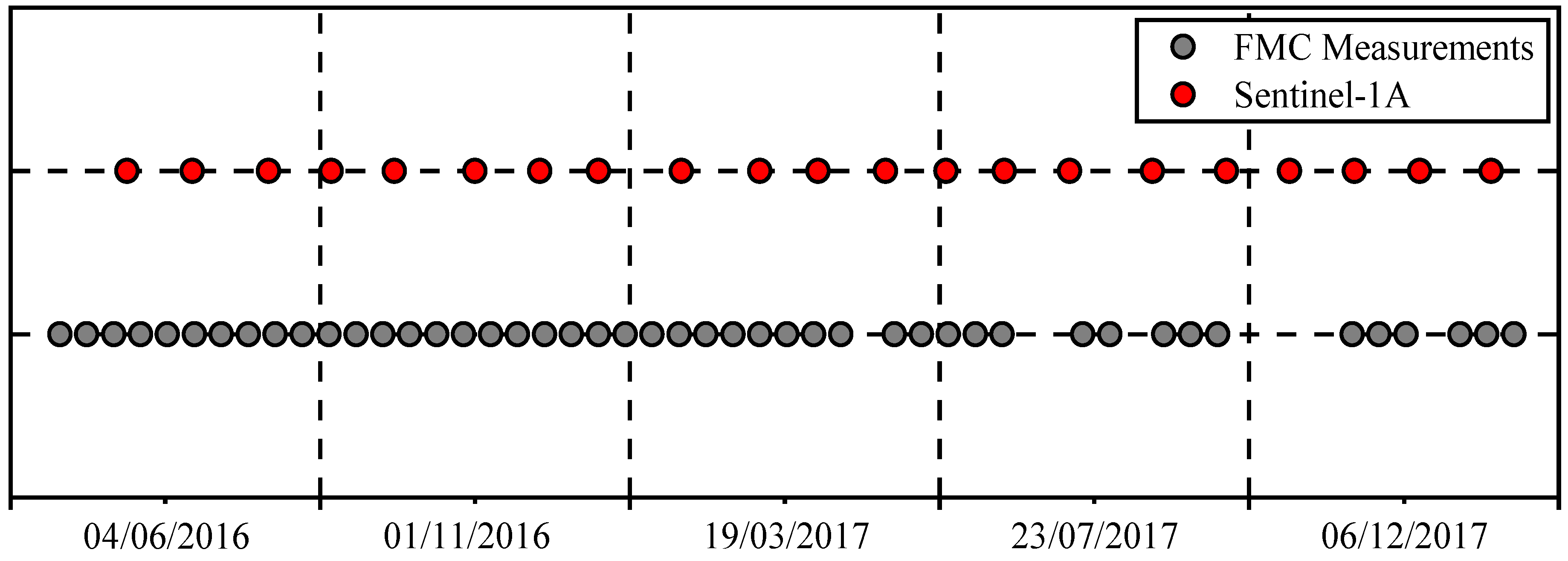
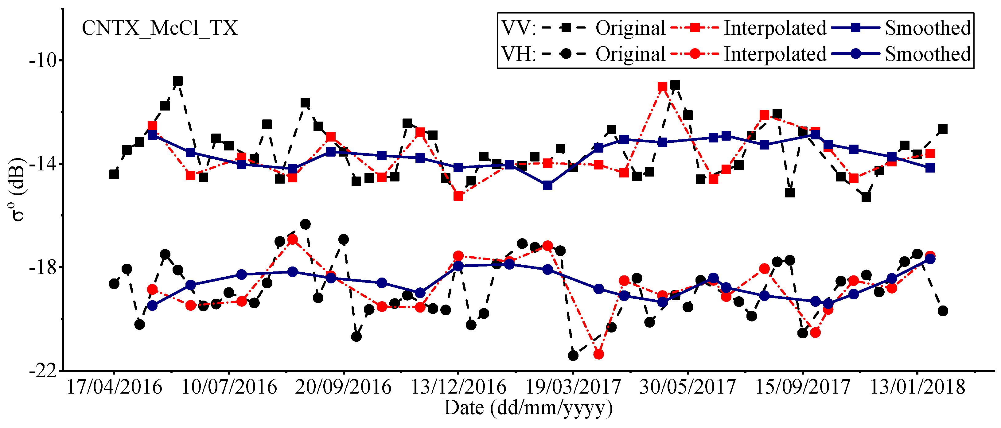
The preprocessing of the Sentinel-1A data includes radiometric correction, speckle noise filtering using refined Lee filter [63], geometric correction with Range–Doppler terrain correction, projection transformation, and resampling to 30 m to reduce the effect of local spatial heterogeneity, which was conducted using the SNAP software 6.0 (https://step.esa.int/main/toolboxes/snap/) provided by ESA. Due to the mismatch between the acquired date of Sentinel-1A and the forest FMC measured date (shown in Figure 3), a cubic spline interpolation method [64] was used to interpolate the original Sentinel-1A data to resolve the backscatter on the forest FMC measured date. Then the Savitzky–Golay smooth filter [65] was applied to smooth the interpolated Sentinel-1A data to eliminate the influence of the time-series noise caused by weather condition and SAR sensor. Both steps were implemented using the built-in function (interp1 and sgolayfilt functions) in Matlab software 2018a. The original, interpolated and smoothed time-series dual polarimetric Sentinel-1A data for this site is shown in Figure 4.
The radar incidence angle has a significant impact on the observed backscatter and thus directly affects the accuracy level of surface variables estimation. To reduce its effect, the theoretical correction method proposed by Ulaby et al. [55], which is based on Lambert’s law [66] for optics, was used to normalize the interpolated and smoothed Sentinel-1A data:
where is the reference radar incidence angle, is the measured radar incidence angle, and represent the VV and VH backscatters at corresponding angle, respectively. The reference radar incidence angle was set as the central angle (43.91°) of acquired Sentinel-1A data.
2.2. FMC Estimation from Sentinel-1A Data
2.2.1. Model Selection and Coupling
The first order radiative transfer model, WCM, was used to retrieve the forest FMC in this study. WCM is a semi-empirical vegetation backscatter model proposed by Attema et al. [53] in 1978, and normally used to simulate the total radar backscatter () from surface vegetation and bare soil [23]. The formulation of this model is expressed as follows (in dB unit):
where is the direct backscatter contribution of surface vegetation layer, is the double-bounce backscatter component between surface vegetation and bare soil, and is the direct bare soil backscatter contribution double attenuated by surface vegetation. is the two-way attenuation of the surface vegetation layer. θ is the reference radar incidence angle (43.91° in this study). V1 and V2 are the scattering and attenuation characters of vegetation layer, respectively. A and B are model empirical coefficients that depend on the vegetation structure type and SAR sensor configuration. Traditionally, the is negligible since its influence on the total backscatter is relatively weak compared with the bare soil and surface vegetation components [47,51]. Therefore, the WCM can be reformulated as:
In this study, the direct bare soil backscatter contribution double attenuated by vegetation layer, , was modelled using the empirical bare soil backscatter linear model proposed by Prévot et al. [32], which considers that the backscatter of bare soil can be directly calculated through a linear function of its surface soil moisture as:
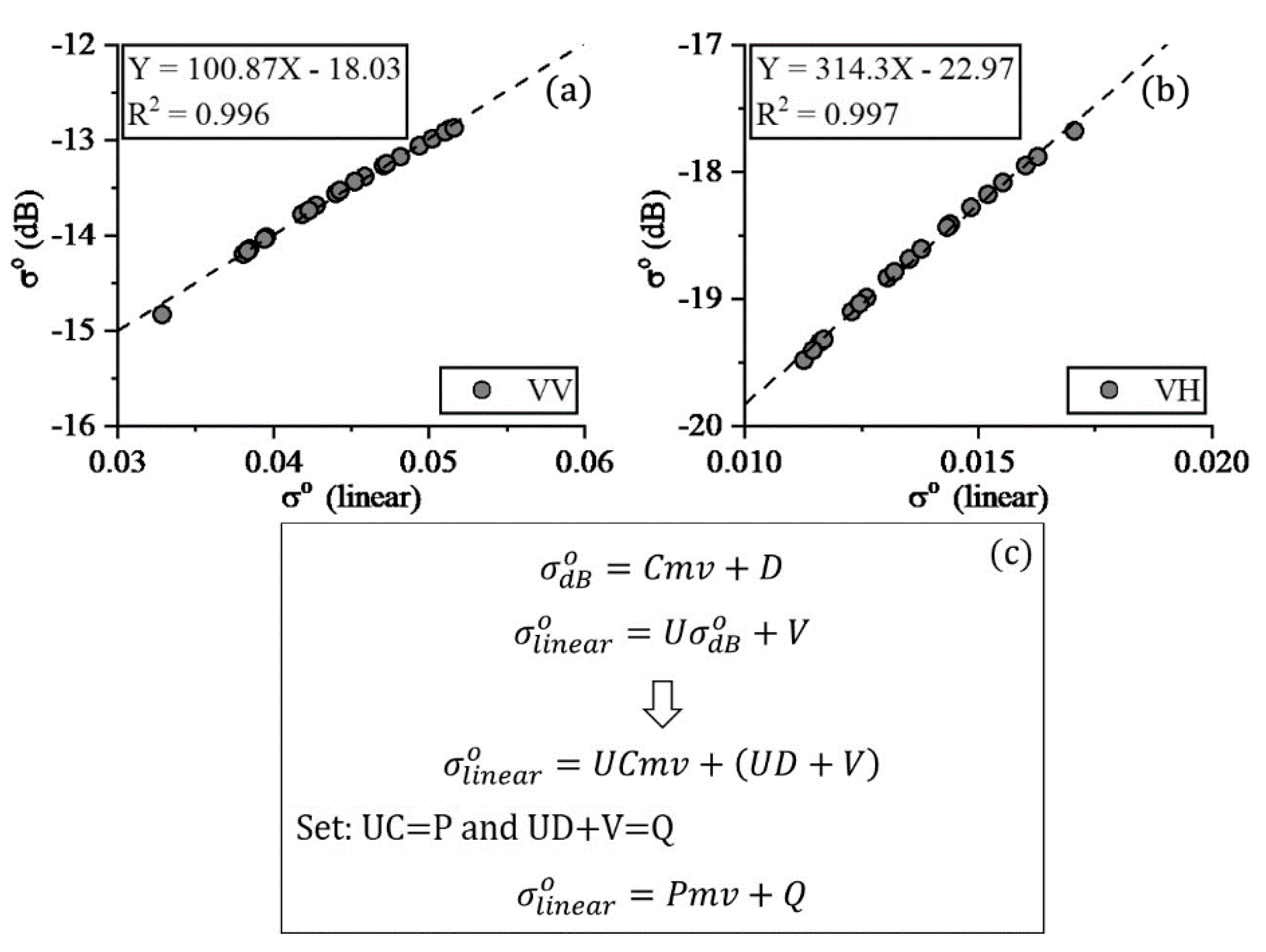
where is the surface soil moisture expressed in volumetric units, C and D are surface roughness-dependent parameters and be determined experimentally for a given SAR sensor. C depends on the sensitivity of the microwave signal to soil moisture and D represents the backscatter contribution of dry soil [32]. Here, it should be noted that the in the bare soil backscatter linear model (Equation (6)) is expressed in dB units while that in the WCM (Equations (2) and (5)) is expressed in linear units, and therefore transformation between these two units was required. From the statistical analysis of the observed backscatter of acquired C-band Sentinel-1A data, we found that backscatter expressed in the dB unit had a strong linear relationship with that expressed in linear unit over a small variation range (shown in Figure 5). Consequently, we used this strong linear relationship (described in Figure 5) to reduce the model complexity introduced by exponential and logarithm forms when coupling the bare soil backscatter linear model into the WCM. Therefore, WCM can be transformed as:
where A, B, P and Q are model empirical coefficients and optimized by the least square method, V1 and V2 are both parameterized by surface vegetation parameter (i.e., the FMC in this study).
The surface soil moisture () in Equation (7) is sensitive to the total radar backscatter and therefore it can introduce high uncertainty when the coupled model comes to retrieve forest FMC in this study. However, this variable is unknown in the FMC measurement site and to date, there is no reliable satellite product or measurements available to parameterize it. Therefore, to reduce the effect of this variable (), the VV and VH dual polarimetric Sentinel-1A data were combined in Equation (7) to eliminate the by:
where and represent the VV and VH backscatters, respectively. AVV, BVV, PVV, QVV and AVH, BVH, PVH, QVH are model coefficients corresponding to VV and VH polarimetric mode. Thus, the final coupled model for forest FMC retrieval can be expressed as:
2.2.2. Model Calibration and Validation
The eight model empirical coefficients (AVV, BVV, PVV, QVV and AVH, BVH, PVH, QVH in Equation (10)) were optimized using the non-linear Levenberg–Marquardt [67] algorithm. To avoid the local optimal solutions produced by the non-linear least square method, 5000 sets of random parameter combinations were used to initialize the model, and the fitting parameters corresponding to the minimum root mean square error (RMSE) between the modelled and measured VH backscatter were regarded as the global optimal solution to retrieve FMC.
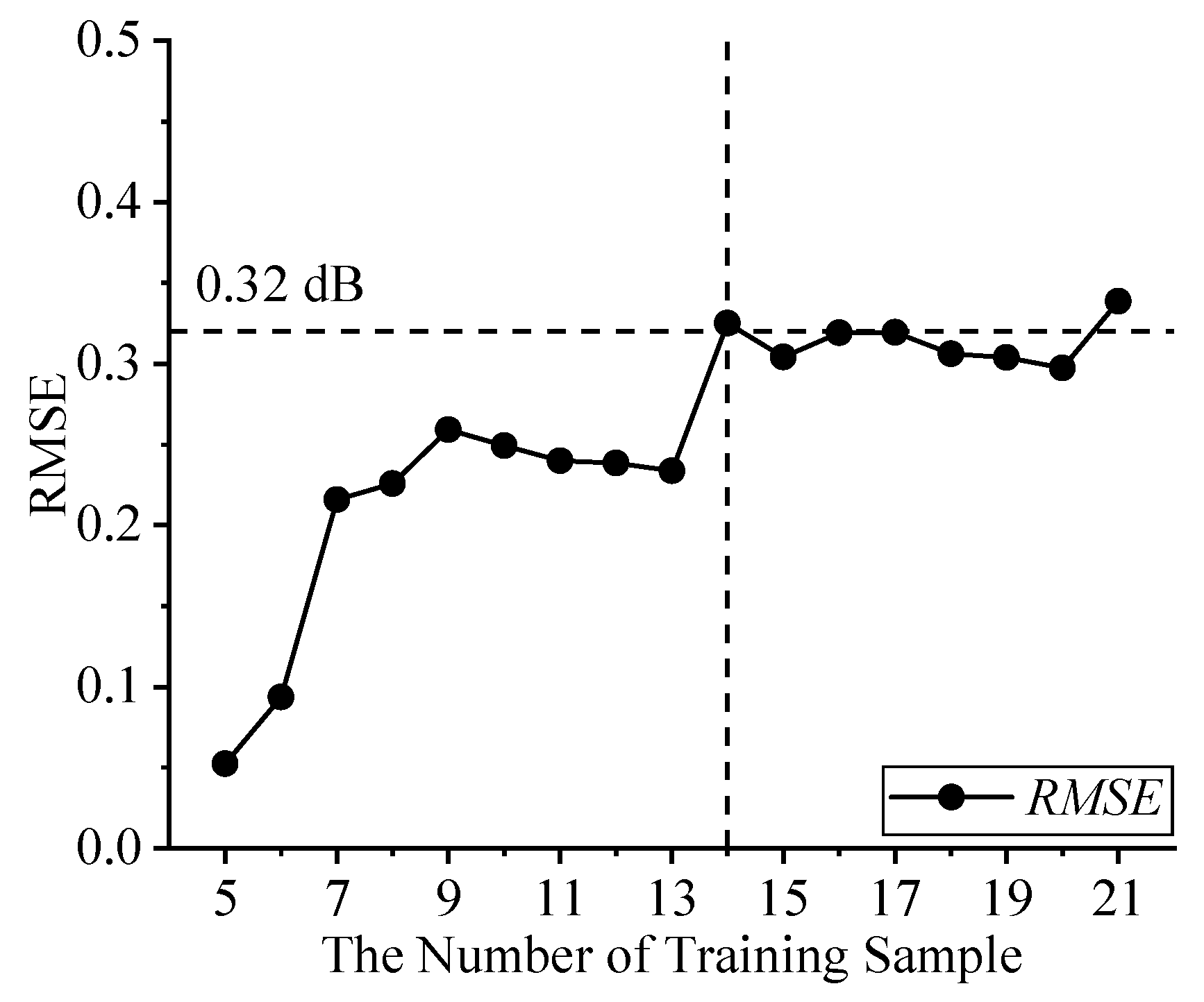
In addition, from the perspective of statistical analysis, an insufficient number in the training sample may result in an overfitting problem when using the non-linear least square method, which may lead to poor predictions [23]. Therefore, to determine the optimal number for the training sample and avoid the overfitting problem, different number of training sample were selected to calibrate the coupled model, and the RMSE between the modelled and measured VH backscatters was selected to evaluate the performance of the model calibration. As is showed in Figure 6, the RMSE showed an upward trend with an increased number in the training sample up to 14; then the RMSE of the model calibration stabilized around 0.32 dB, indicating that the overfitting problem was alleviated. Consequently, a three-fold cross-validation method was presented to fit Equation (10) and validation of retrieved FMC by dividing all the measurements taken at the study site into equally three samples (i.e., each sample comprised 7 FMC measurements). Two samples (i.e., the training sample) were used for the model calibration (Equation (10)), and the other sample (i.e., the testing sample) was used for the validation. The process was repeated for three times to adequately test the performance of the presented Sentinel-1A data-based method.
2.2.3. Look-up Table (LUT) Building and FMC Retrieval
Due to the complexity of Equation (10), an analytical solution of FMC cannot be directly derived from the VV and VH backscatters. Consequently, a LUT methodology was used to obtain the optimal FMC from the observed backscatters. The LUT was built by running the calibrated coupled model (Equation (10)) forward with two inputs (FMC and VV backscatter), and then the corresponding output, the modelled VH backscatter, was generated. The range of FMC in LUT was set based on field forest FMC measurements (70 %–150 %), and the VV backscatter was directly obtained from the Sentinel-1A data in the testing sample.
Once the LUT was built, FMC was retrieved using a cost function to search the best fitted VH backscatter in the LUT from the observed Sentinel-1A VH backscatter. In this study, MAEr, defined as the absolute difference of the modelled and measured VH backscatters, was selected as the cost function and defined as:
where and represent the modelled and measured VH backscatters.
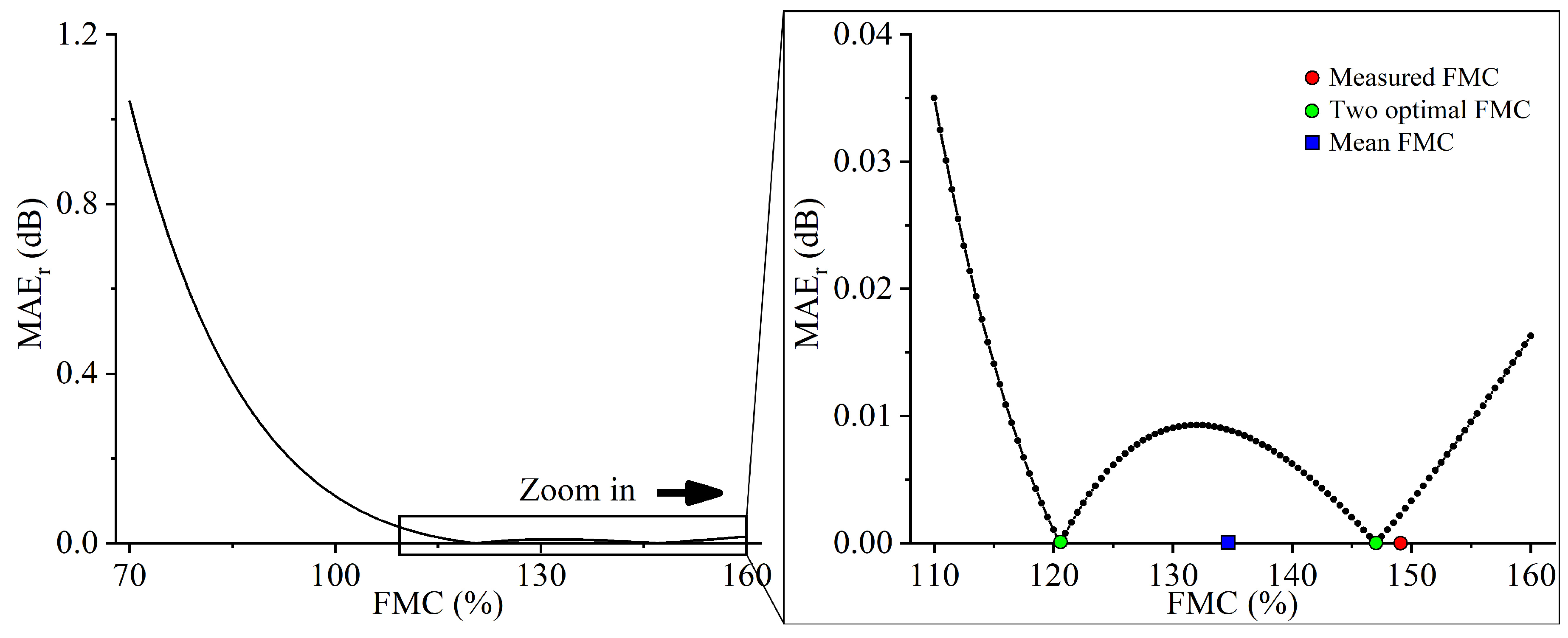
However, the LUT inversion method is generally hampered by the ill-posed inversion problem, meaning that different input parameter combinations (i.e., FMC and VV backscatter) may correspond to almost identical output (i.e., VH backscatter), and would dramatically decrease the accuracy level of retrieved parameters (i.e., forest FMC) [11,68]. For instance, Figure 7 shows an example of the ill-posed inversion problem where two minimum FMC values (green points with 121 % and 147 %) can be obtained with the lowest MAEr between the modelled and measured VH backscatters. The ground measured FMC is 149 % (red point), which is closer to the green dot on the right (FMC = 147 %), than the green dot on the left (FMC = 121 %) and the mean of both green dots (blue point, FMC = 134 %). This phenomenon seriously raises the question about how to choose the final solution to the inversion from these solutions.
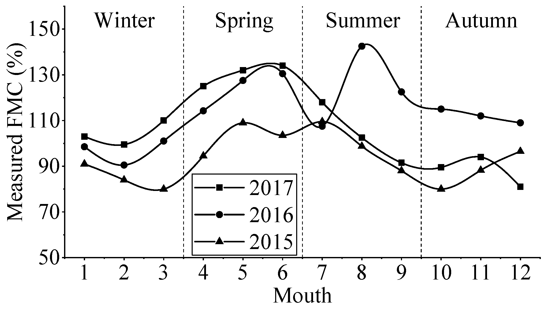
Previous studies showed that the use of prior knowledge (such as the ranges of free parameters and their distributions from field measurements or remote sensing products, and the vegetation canopy type structure) is an efficient way to alleviate the ill-posed inversion problem [68]. In this study, we found that the time-series FMC measurements of this study site in 2015, 2016 and 2017 showed a strongly seasonal phenological feature of high and low FMC values among different periods (Figure 8). Thus, this feature was introduced into the retrieval procedure to alleviate the ill-posed inversion problem: for the high-FMC periods (spring and summer), the higher FMC value corresponding the lowest MAEr was selected as the optimal retrieved FMC, and for the low-FMC period (autumn and winter), the lower FMC value corresponding the lowest MAEr was selected as the optimal retrieved FMC.
2.3. FMC Estimation from Landsat 8 OLI Data
The presented Sentinel-1A data-based methodology for forest FMC retrieval was compared with the retrievals using optical Landsat 8 OLI data and the empirical PLSR method since both data have similar spatial resolution (Sentinel-1A data: 5 × 20 m for azimuth and range resolution; Landsat 8 OLI data: 30 m), which will reduce the effect of spatial heterogeneity.
Optical Landsat 8 OLI surface reflectance data in the study site was extracted using the Google Earth Engine tool [69]. To resolve the optical Landsat 8 OLI reflectance data on field forest FMC measurements date, the extracted time-series Landsat 8 OLI data were similarly interpolated and smoothed by the cubic spline interpolation method [64] and the Savitzky-Golay smooth filter [65]. Then, the reflectance data on field forest FMC measurements date was used to estimate FMC using the PLSR method following Quan et al. [70]. To adequately compare with the results using the presented Sentinel-1A data-based methodology, the empirical PLSR model was also trained and tested using the three-fold cross-validation method described in Section 2.2.2. Two of these three parts were used for training the PLSR model and the other one part for testing, and this was repeated three times.
PLSR is a statistical method that bears relation to principal components regression. Instead of finding hyperplanes of maximum variance between the response and independent variables, it finds a linear regression model by projecting the predicted variables and the observable variables to a new space. This technique reduces a large number of measured variables to a few non-correlated latent variables while maximizing co-variability to the variable(s) of interest. PLSR is particularly suited when the matrix of predictors has more variables than observations [11,71]. The aim of PLSR is to build a linear model such as the following:
where Y is the vector of the response variable (i.e., forest FMC), X is the predictor matrix (i.e., Landsat 8 surface reflectance data, Band 2 to 7, since visible and infrared bands are sensitive to FMC [11]), is the model coefficients matrix, and E is the residuals matrix. In principle, PLSR is closely associated with the principal component analysis regression (PCAR), but PCAR performs the decomposition on the predictor matrix (X) alone. PLSR uses the vector of response variable during the decomposition process and performs the decomposition on both the predictor matrix (X) and response variable vector (Y) simultaneously. This procedure can reduce the number of X and Y to a few independent variables.
3. Results
3.1. FMC Estimated Results from Sentinel-1A Data
Figure 9 shows the scatterplots between modelled and measured VH backscatters using the three-fold cross-validation method. It can be found that the VH backscatter of training sample was correctly modelled by the presented coupled model as illustrated by a low RMSE value when compared to the measured VH backscatter (0.33 dB (sample 1), 0.34 dB (sample 2) and 0.35 dB (sample 3)), indicating that the calibrated coupled model (Equation 10) can well simulate the backscatter situation of surface. A LUT was then generated by running the model forwardly, and the observed VH backscatter of the testing sample was used to retrieve forest FMC. Figure 10 shows the scatterplots between estimated and measured forest FMC using the three-fold cross-validation method. Overall, it can be concluded that the forest FMC measurements at the study site were accurately estimated, with RMSE between measured and estimated forest FMC of 19.53% (Sample 1), 12.64% (Sample 2) and 15.45% (Sample 3). Figure 11 shows the time-series distribution of estimated and measured forest FMC of the study site. Although the estimated FMC may be higher or lower than the measured forest FMC, the time-series trend of measured forest FMC is reproduced well by the estimated FMC.
3.2. FMC Estimated Results from Landsat 8 OLI Data
As a comparison, the Landsat 8 OLI data was also used to retrieve forest FMC using the PLSR method in the study site. Figure 12 shows the scatterplots between estimated and measured forest FMC using the three-fold cross-validation method, and Table 1 lists the corresponding RMSE of PLSR model training and testing. From Figure 12 and Table 1, it is obvious that although the accuracy level of PLSR model training is satisfactory (RMSE of three training samples are less than 10% and the corresponding scatterplots are distributed around the 1:1 line), the estimated results using the testing sample were not acceptable with a higher RMSE (approximately 24%) and the seriously deviated scatterplots with regard to the 1:1 line.
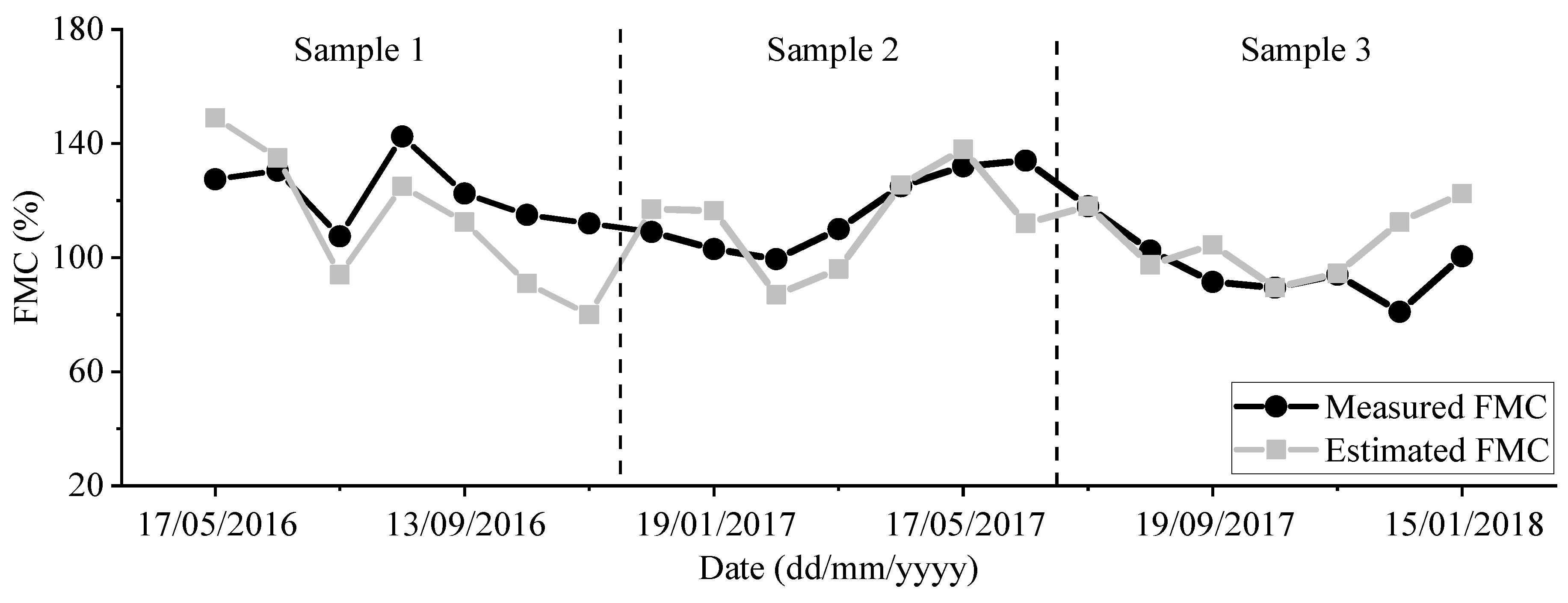
Compared with the forest FMC estimated results using the presented Sentinel-1A data-based method (Figure 9 and Figure 10), FMC was poorly estimated using the Landsat 8 OLI data and the PLSR method, with the RMSE between estimated and measured forest FMC being 20.11% (Sample 1), 26.21% (Sample 2) and 26.73% (Sample 3). Figure 13 shows the time-series distribution of estimated and measured forest FMC. It was found that the time-series trend of estimated forest FMC was not well fitted along with the measured one when compared with Figure 11.
4. Discussion
Current studies so far for forest FMC retrievals are generally based on the optical remote sensing data from multiple sensors since the vegetation liquid water has strong absorption character in the near-infrared and shortwave-infrared bands [3,17]. In this content, Jurdao et al. [2] utilized the PRO-GeoSail RTM and MODIS data to retrieve forest FMC, obtaining RMSE between estimated and measured forest FMC of 27.7% over the Mediterranean and 28.7% over the Eurosiberian regions. Similar errors (RMSE = 26.28%) was also found by Yebra et al. [7] over an Oak forest using the MODIS data and PROSAILH RTM. Quan et al. [11] coupled the PROSAIL and PRO-GeoSail RTMs to retrieve forest FMC from Landsat 8 OLI data, with an RMSE of 32.35% in the Sichuan province, China. Caccamo et al. [6] calibrated an empirical statistical model based on the normalized difference infrared index-band 6 (NDII6) and the maximum-minimum normalization of visible atmospherically resistant index (VARI) from MODIS data to monitor FMC of three vegetation types, including shrubland, heathland and sclerophyll forest, in south-eastern Australia, and provided a good results for forest FMC estimation. Adab et al. [72] estimated forest FMC from Landsat 7 data and MODIS data using multiple linear regression (MLR) and artificial neural network (ANN) method in the northern Iran (Northeastern Hyrcanian forests), providing good results for forest FMC estimation (RMSE = 24.4% (MLR + Landsat 7), 15.6% (ANN + Landsat 7), 50.2% (MLR + MODIS) and 48% (ANN + MODIS)). In this study, the empirical bare soil backscatter linear model was coupled into the semi-empirical vegetation backscatter WCM to retrieve forest FMC from time-series of dual polarimetric (VV/VH) C-band Sentinel-1A data, and its performance was validated using the field forest FMC measurements taken in Texas, USA. We obtained an RMSE between estimated and measured FMC of 19.53% (Sample 1), 12.64% (Sample 2) and 15.45% (Sample 3), that were within the range of RMSE region reported in these previous literatures. Additionally, as a comparison, the optical Landsat 8 OLI data was implemented to estimate the forest FMC in the same field FMC measurements site using the empirical PLSR method, achieving a higher RMSE between estimated and measured forest FMC (20.11% (Sample 1), 26.21% (Sample 2) and 26.73% (Sample 3)). Consequently, in this study, we demonstrated a huge potential usage of C-band Sentinel-1A data for forest FMC estimation in comparison with the previous research that used optical remote sensing data.
Studies focused on FMC estimation using SAR data were still rarely reported at present. Leblon et al. [24] analyzed the relationship between measured FMC and SAR backscatter for white spruce from C-band ERS-1 data in the Mackenzie River basin, northwest Canada, and obtained a coefficient of determination R2 between observed backscatter and measured FMC of 0.461. Tanase et al. [25] used the linear regression method to estimate FMC from L-band airborne SAR data in the Murrumbidgee catchment, Australia, obtaining R2 and RMSE between estimated and measured FMC of 0.34–0.70 and 10 %–15 %, respectively. These two studies based on SAR data made use of an empirical model that linked the field FMC measurements to the SAR backscatter. However, the completed empirical model may have the shortcoming of being site-specific and sensor-dependent. Compared with these two above studies, the forest FMC estimation method presented in this study, coupled the empirical bare soil backscatter linear model and the semi-empirical vegetation backscatter WCM, is expected to be more reproducible and robust since it introduces the physical mechanism of surface vegetation microwave backscatter to establish the total surface backscatter model [32,73].
One of the critical obstacles hampering the accurate retrieval of forest FMC in this study was the ill-posed inversion problem. To alleviate this effect, the seasonal phenological feature of FMC was introduced as the prior information to constrain the inversion result. However, this prior information depended on the seasonal phenological feature in terms of local FMC conditions that may lack generality. Therefore, a more reasonable and reproducible strategy to alleviate the ill-posed inversion problem should be furtherly explored. Hosseini et al. [31] adopted surface soil moisture as a priori knowledge to obtain the optimal LAI form C-band Randarsat-2 data and L-band airborne SAR data over an agricultural region located in Canada. Fan et al. [18] found that FMC had a positive correlation with surface soil moisture since the main effects of surface soil moisture deficit on plant condition were exerted through the plant water potential, which in turn affected the relative water of plant tissue. Nolan et al. [74] also found that the live FMC for Mediterranean mixed forest in Catalonia, Spain, were most reliant on shallow soil water. Therefore, the introduction of surface soil moisture may be an alternative effective strategy to improve the performance of the model presented here, which will be furtherly explored in the near future.
To our knowledge, the dual-polarimetric C-band Sentinel-1A data is the only free satellite SAR product to date, and it has been downloadable since October 2014, however, only the VV & VH polarimetric modes are available freely. Tanase et al. [25] discussed the statistical relationship between field FMC measurements and radar backscatters of different polarimetric modes (HH, HV and VV) in semiarid environments using L-band airborne SAR data. Their study demonstrated the statistical relationship between FMC and radar backscatter of different polarimetric modes is different since the microwave signal with different polarimetric modes reflects different scattering characteristic of the ground object. Therefore, if more polarimetric data (i.e., VV, VH, HV and HH) can be available freely in time-series, the performance of the presented SAR data-based method for forest FMC estimation can be furtherly explored.
5. Conclusions
In this study, a methodology using dual polarimetric C-band Sentinel-1A data for forest FMC retrieval was presented by coupling the empirical bare soil backscatter linear model and the semi-empirical vegetation backscatter WCM. To alleviate the ill-posed inversion problem, the seasonal phenological feature of field forest FMC measurements was used as the effective prior information to constrain the inversion process. The three-fold cross-validation method was adopted to verify the performance of the presented method for forest FMC retrieval. Compared with the field forest FMC measurements, the results using the Sentinel-1A data-based method presented in this study showed a good accuracy level, with RMSE between estimated and measured forest FMC of 19.53% (Sample 1), 12.64% (Sample 2) and 15.45% (Sample 3), that is within the range of accuracy reported in previous literature for forest FMC retrieval. In addition, to adequately verify the effectiveness of the presented Sentinel-1A data-based method for forest estimation, the Landsat 8 OLI data and empirical PLSR method was also adopted. The results show that the presented Sentinel-1A data-based method well reproduced the time-series trend of measured forest FMC and performed a better accuracy level than Landsat 8-based method with RMSE of 20.11% (Sample 1), 26.21% (Sample 2) and 26.73% (Sample 3). These results show the possibility of developing an operational method based on satellite SAR data to estimate forest FMC and provides good prospects to develop an operational framework for global scale FMC mapping.
Author Contributions
B.H. and X.Q. supervised and fund this research; L.W., X.Q. and B.H. conceived and designed the experiments; L.W. performed the experiments and analyzed the data; L.W. and X.Q. wrote the first version of the manuscript; M.Y. refined the methodology and contributed to the final version of the manuscript; M.X. and X.L. edited the manuscript.
Funding
This work was supported by the National Natural Science Foundation of China (Contract No. 41671361 and 41801272) and the Fundamental Research for the Central Universities (Contract No. ZYGX2017KYQD195).
Acknowledgments
The authors would like to thank the ESA and the NFMD for providing the Sentinel-1A data and field FMC measurements, respectively.
Conflicts of Interest
The authors declare no conflict of interest.
Appendix A

Table A1.
The time-series field FMC measurements in CNTX_McCl_TX site.
| No. | Date(dd/mm/yyyy) | FMC (%) | No. | Date(dd/mm/yyyy) | FMC (%) |
|---|---|---|---|---|---|
| 1 | 15/05/2016 | 127.5 | 12 | 20/04/2017 | 125.0 |
| 2 | 15/06/2016 | 130.5 | 13 | 17/05/2017 | 132.0 |
| 3 | 19/07/2016 | 107.5 | 14 | 12/06/2017 | 134.0 |
| 4 | 16/08/2016 | 142.5 | 15 | 11/07/2017 | 118.0 |
| 5 | 13/09/2016 | 122.5 | 16 | 17/08/2017 | 102.5 |
| 6 | 19/10/2016 | 115.5 | 17 | 19/09/2017 | 91.5 |
| 7 | 17/11/2016 | 112.0 | 18 | 17/10/2017 | 89.5 |
| 8 | 13/12/2016 | 109.0 | 19 | 15/11/2017 | 94.0 |
| 9 | 19/01/2017 | 103.0 | 20 | 14/12/2017 | 81.0 |
| 10 | 23/02/2017 | 99.5 | 21 | 15/01/2018 | 100.5 |
| 11 | 21/03/2017 | 110.0 | - | - | - |
References
- Chuvieco, E.; Riano, D.; Aguado, I.; Cocero, D. Estimation of fuel moisture content from multitemporal analysis of Landsat Thematic Mapper reflectance data: applications in fire danger assessment. Int. J. Remote Sens. 2002, 23, 2145–2162. [Google Scholar] [CrossRef]
- Jurdao, S.; Yebra, M.; Guerschman, J.P.; Chuvieco, E. Regional estimation of woodland moisture content by inverting Radiative Transfer Models. Remote Sens. Environ. 2013, 132, 59–70. [Google Scholar] [CrossRef]
- Yebra, M.; Dennison, P.E.; Chuvieco, E.; Riaño, D.; Zylstra, P.; Jr, E.R.; Danson, F.M.; Qi, Y.; Jurdao, S. A global review of remote sensing of live fuel moisture content for fire danger assessment: Moving towards operational products. Remote Sens. Environ. 2013, 136, 455–468. [Google Scholar] [CrossRef]
- Chladil, M.A.; Nunez, M. Assessing Grassland Moisture and Biomass in Tasmania - the Application of Remote-Sensing and Empirical-Models for a Cloudy Environment. Int. J. Wildland Fire. 1995, 5, 165–171. [Google Scholar] [CrossRef]
- Paltridge, G.W.; Barber, J. Monitoring grassland dryness and fire potential in australia with NOAA/AVHRR data. Remote Sens. Environ. 1988, 25, 381–394. [Google Scholar] [CrossRef]
- Caccamo, G.; Chisholm, L.; Bradstock, R.; Puotinen, M.L.; Pippen, B. Monitoring live fuel moisture content of heathland, shrubland and sclerophyll forest in south-eastern Australia using MODIS data. Int. J. Wildland Fire 2012, 21, 257–269. [Google Scholar] [CrossRef]
- Yebra, M.; Chuvieco, E. Generation of a Species-Specific Look-Up Table for Fuel Moisture Content Assessment. IEEE J. Sel. Top. Appl. Earth Obs. Remote Sens. 2009, 2, 21–26. [Google Scholar] [CrossRef]
- Yebra, M.; Chuvieco, E. Linking ecological information and radiative transfer models to estimate fuel moisture content in the Mediterranean region of Spain: Solving the ill-posed inverse problem. Remote Sens. Environ. 2009, 113, 2403–2411. [Google Scholar] [CrossRef]
- Yebra, M.; Quan, X.; Riaño, D.; Rozas Larraondo, P.; van Dijk, A.I.J.M.; Cary, G.J. A fuel moisture content and flammability monitoring methodology for continental Australia based on optical remote sensing. Remote Sens. Environ. 2018, 212, 260–272. [Google Scholar] [CrossRef]
- Yilmaz, M.T.; Jr, E.R.H.; Goins, L.D.; Ustin, S.L.; Vanderbilt, V.C.; Jackson, T.J. Vegetation water content during SMEX04 from ground data and Landsat 5 Thematic Mapper imagery. Remote Sens. Environ. 2008, 112, 350–362. [Google Scholar] [CrossRef] [Green Version]
- Quan, X.; He, B.; Yebra, M.; Yin, C.; Liao, Z.; Li, X. Retrieval of forest fuel moisture content using a coupled radiative transfer model. Environ. Model. Softw. 2017, 95, 290–302. [Google Scholar] [CrossRef]
- Quan, X.W.; He, B.B.; Li, X.; Liao, Z.M. Retrieval of Grassland Live Fuel Moisture Content by Parameterizing Radiative Transfer Model With Interval Estimated LAI. IEEE J. Sel. Top. Appl. Earth Observ. Remote Sens. 2016, 9, 910–920. [Google Scholar] [CrossRef]
- Yebra, M.; Chuvieco, E.; Riano, D. Estimation of live fuel moisture content from MODIS images for fire risk assessment. Agric. For. Meteorol. 2008, 148, 523–536. [Google Scholar] [CrossRef]
- Chuvieco, E.; Cocero, D.; Riano, D.; Martin, P.; Martinez-Vega, J.; de la Riva, J.; Perez, F. Combining NDVI and surface temperature for the estimation of live fuel moisture content in forest fire danger rating. Remote Sens. Environ. 2004, 92, 322–331. [Google Scholar] [CrossRef]
- Casas, A.; Riano, D.; Ustin, S.L.; Dennison, P.; Salas, J. Estimation of water-related biochemical and biophysical vegetation properties using multitemporal airborne hyperspectral data and its comparison to MODIS spectral response. Remote Sens. Environ. 2014, 148, 28–41. [Google Scholar] [CrossRef]
- Myoung, B.; Kim, S.H.; Nghiem, S.V.; Jia, S.; Kafatos, M.C. Estimating Live Fuel Moisture from MODIS Satellite Data for Wildfire Danger Assessment in Southern California USA. Remote Sens. 2018, 10, 87. [Google Scholar] [CrossRef]
- Bowyer, P.; Danson, F.M. Sensitivity of spectral reflectance to variation in live fuel moisture content at leaf and canopy level. Remote Sens. Environ. 2004, 92, 297–308. [Google Scholar] [CrossRef]
- Fan, L.; Wigneron, J.-P.; Xiao, Q.; Al-Yaari, A.; Wen, J.; Martin-StPaul, N.; Dupuy, J.-L.; Pimont, F.; Al Bitar, A.; Fernandez-Moran. Evaluation of microwave remote sensing for monitoring live fuel moisture content in the Mediterranean region. Remote Sens. Environ. 2018, 205, 210–223. [Google Scholar] [CrossRef]
- Entekhabi, D.; Njoku, E.G.; O’Neill, P.E.; Kellogg, K.H.; Crow, W.T.; Edelstein, W.N.; Entin, J.K.; Goodman, S.D.; Jackson, T.J.; Johnson, J. The soil moisture active passive (SMAP) mission. Proc. IEEE 2010, 98, 704–716. [Google Scholar] [CrossRef]
- Aubert, M.; Baghdadi, N.N.; Zribi, M.; Ose, K.; El Hajj, M.; Vaudour, E.; Gonzalez-Sosa, E. Toward an operational bare soil moisture mapping using TerraSAR-X data acquired over agricultural areas. IEEE J. Sel. Top. Appl. Earth Obs. Remote Sens. 2013, 6, 900–916. [Google Scholar] [CrossRef]
- Bai, X.; He, B.; Li, X. Optimum surface roughness to parameterize advanced integral equation model for soil moisture retrieval in prairie area using Radarsat-2 data. IEEE Trans. Geosci. Remote Sens. 2016, 54, 2437–2449. [Google Scholar] [CrossRef]
- Bai, X.; He, B. Potential of Dubois model for soil moisture retrieval in prairie areas using SAR and optical data. Int. J. Remote Sens. 2015, 36, 5737–5753. [Google Scholar] [CrossRef]
- Bai, X.; He, B.; Li, X.; Zeng, J.; Wang, X.; Wang, Z.; Zeng, Y.; Su, Z. First assessment of Sentinel-1A data for surface soil moisture estimations using a coupled Water Cloud Model and Advanced Integral Equation Model over the Tibetan Plateau. Remote Sens. 2017, 9, 714. [Google Scholar] [CrossRef]
- Leblon, B.; Kasischke, E.; Alexander, M.; Doyle, M.; Abbott, M. Fire Danger Monitoring Using ERS-1 SAR Images in the Case of Northern Boreal Forests. Nat. Hazards. 2002, 27, 231–255. [Google Scholar] [CrossRef]
- Tanase, M.; Panciera, R.; Lowell, K.; Aponte, C. Monitoring live fuel moisture in semiarid environments using L-band radar data. Int. J. Wildland Fire. 2015, 24, 560–572. [Google Scholar] [CrossRef]
- Breit, H.; Fritz, T.; Balss, U.; Lachaise, M.; Niedermeier, A.; Vonavka, M. TerraSAR-X SAR processing and products. IEEE Trans. Geosci. Remote Sens. 2010, 48, 727–740. [Google Scholar] [CrossRef]
- Das, K.; Paul, P.K. Soil moisture retrieval model by using RISAT-1, C-band data in tropical dry and sub-humid zone of Bankura district of India. Egypt. J. Remote Sens. Space Sci. 2015, 18, 297–310. [Google Scholar] [CrossRef] [Green Version]
- Gherboudj, I.; Magagi, R.; Berg, A.A.; Toth, B. Soil moisture retrieval over agricultural fields from multi-polarized and multi-angular RADARSAT-2 SAR data. Remote Sens. Environ. 2011, 115, 33–43. [Google Scholar] [CrossRef]
- Rosenqvist, A.; Shimada, M.; Suzuki, S.; Ohgushi, F.; Tadono, T.; Watanabe, M.; Tsuzuku, K.; Watanabe, T.; Kamijo, S.; Aoki, E. Operational performance of the ALOS global systematic acquisition strategy and observation plans for ALOS-2 PALSAR-2. Remote Sens. Environ. 2014, 155, 3–12. [Google Scholar] [CrossRef]
- Malenovský, Z.; Rott, H.; Cihlar, J.; Schaepman, M.E.; García-Santos, G.; Fernandes, R.; Berger, M. Sentinels for science: Potential of Sentinel-1, -2, and -3 missions for scientific observations of ocean, cryosphere, and land. Remote Sens. Environ. 2012, 120, 91–101. [Google Scholar] [CrossRef]
- Hosseini, M.; Mcnairn, H.; Merzouki, A.; Pacheco, A. Estimation of Leaf Area Index (LAI) in corn and soybeans using multi-polarization C- and L-band radar data. Remote Sens. Environ. 2015, 170, 77–89. [Google Scholar] [CrossRef]
- Prévot, L.; Champion, I.; Guyot, G. Estimating surface soil moisture and leaf area index of a wheat canopy using a dual-frequency (C and X bands) scatterometer. Remote Sens. Environ. 1993, 46, 331–339. [Google Scholar] [CrossRef]
- Ulaby, F.T.; Batlivala, P.P.; Dobson, M.C. Microwave backscatter dependence on surface roughness, soil moisture, and soil texture: Part I-bare soil. IEEE Trans. Geosci. Electron. 1978, 16, 286–295. [Google Scholar] [CrossRef]
- Bernard, R.; Martin, P.; Thony, J.; Vauclin, M.; Vidal-Madjar, D. C-band radar for determining surface soil moisture. Remote Sens. Environ. 1982, 12, 189–200. [Google Scholar] [CrossRef]
- Oh, Y.; Sarabandi, K.; Ulaby, F.T. An empirical model and an inversion technique for radar scattering from bare soil surfaces. IEEE Trans. Geosci. Remote Sens. 1992, 30, 370–381. [Google Scholar] [CrossRef]
- Oh, Y.; Sarabandi, K.; Ulaby, F.T. An inversion algorithm for retrieving soil moisture and surface roughness from polarimetric radar observation. In Proceedings of the Geoscience and Remote Sensing Symposium. IGARSS’94. Surface and Atmospheric Remote Sensing: Technologies, Data Analysis and Interpretation, International, Pasadena, CA, USA, 8–12 August 1994; pp. 1582–1584. [Google Scholar]
- Oh, Y.; Sarabandi, K.; Ulaby, F.T. Semi-empirical model of the ensemble-averaged differential Mueller matrix for microwave backscattering from bare soil surfaces. IEEE Trans. Geosci. Remote Sens. 2002, 40, 1348–1355. [Google Scholar] [CrossRef] [Green Version]
- Oh, Y. Quantitative retrieval of soil moisture content and surface roughness from multipolarized radar observations of bare soil surfaces. IEEE Trans. Geosci. Remote Sens. 2004, 42, 596–601. [Google Scholar] [CrossRef]
- Dubois, P.C.; Van Zyl, J.; Engman, T. Measuring soil moisture with imaging radars. IEEE Trans. Geosci. Remote Sens. 1995, 33, 915–926. [Google Scholar] [CrossRef] [Green Version]
- Panciera, R.; Tanase, M.A.; Lowell, K.; Walker, J.P. Evaluation of IEM, Dubois, and Oh radar backscatter models using airborne L-band SAR. IEEE Trans. Geosci. Remote Sens. 2014, 52, 4966–4979. [Google Scholar] [CrossRef]
- Shi, J.; Wang, J.; Hsu, A.; O’Neili, P.; Engman, E. Estimation of soil moisture and surface roughness parameters using L-band SAR measurements. In Proceedings of the Geoscience and Remote Sensing Symposium, IGARSS’95.‘Quantitative Remote Sensing for Science and Applications’, International, Firenze, Italy, 10–14 July 1995; pp. 507–509. [Google Scholar]
- Shi, J.; Dozier, J. Estimation of snow water equivalence using SIR-C/X-SAR. I. Inferring snow density and subsurface properties. IEEE Trans. Geosci. Remote Sens. 2000, 38, 2465–2474. [Google Scholar] [Green Version]
- Baghdadi, N.; Choker, M.; Zribi, M.; Hajj, M.E.; Paloscia, S.; Verhoest, N.E.; Lievens, H.; Baup, F.; Mattia, F. A new empirical model for radar scattering from bare soil surfaces. Remote Sens. 2016, 8, 920. [Google Scholar] [CrossRef]
- Fung, A.K.; Li, Z.; Chen, K.S. Backscattering from a randomly rough dielectric surface. IEEE Trans. Geosci. Remote Sens. 1992, 30, 356–369. [Google Scholar] [CrossRef]
- Fung, A.K.; Chen, K.-S.; Chen, K. Microwave Scattering and Emission Models for Users; Artech house: Norwood, MA, USA, 2010. [Google Scholar]
- Chen, K.-S.; Wu, T.-D.; Tsang, L.; Li, Q.; Shi, J.; Fung, A.K. Emission of rough surfaces calculated by the integral equation method with comparison to three-dimensional moment method simulations. IEEE Trans. Geosci. Remote Sens. 2003, 41, 90–101. [Google Scholar] [CrossRef]
- He, B.; Xing, M.; Bai, X. A synergistic methodology for soil moisture estimation in an alpine prairie using radar and optical satellite data. Remote Sens. 2014, 6, 10966–10985. [Google Scholar] [CrossRef]
- Wang, L.; He, B.; Bai, X.; Xing, M. Assessment of Different Vegetation Parameters for Parameterizing the Coupled Water Cloud Model and Advanced Integral Equation Model for Soil Moisture Retrieval Using Time Series Sentinel-1A Data. Photogramm. Eng. Remote Sens. 2019, 85, 43–54. [Google Scholar] [CrossRef]
- Ma, Y.; Xing, M.; Ni, X.; Wang, J.; Shang, J.; Zhou, J. Using a Modified Water Cloud Model to Retrive Leaf Area Index (LAI) from Radarsat-2 SAR Data Over an Agriculture Area. In Proceedings of the IGARSS 2018-2018 IEEE International Geoscience and Remote Sensing Symposium, Valencia, Spain, 22 July 2018; pp. 5437–5440. [Google Scholar]
- Joseph, A.T.; van der Velde, R.; O’Neill, P.E.; Lang, R.H.; Gish, T. Soil moisture retrieval during a corn growth cycle using L-band (1.6 GHz) radar observations. IEEE Trans. Geosci. Remote Sens. 2008, 46, 2365–2374. [Google Scholar] [CrossRef]
- Joseph, A.; van der Velde, R.; O’neill, P.; Lang, R.; Gish, T. Effects of corn on C-and L-band radar backscatter: A correction method for soil moisture retrieval. Remote Sens. Environ. 2010, 114, 2417–2430. [Google Scholar] [CrossRef]
- El Hajj, M.; Baghdadi, N.; Zribi, M.; Belaud, G.; Cheviron, B.; Courault, D.; Charron, F. Soil moisture retrieval over irrigated grassland using X-band SAR data. Remote Sens. Environ. 2016, 176, 202–218. [Google Scholar] [CrossRef] [Green Version]
- Attema, E.; Ulaby, F.T. Vegetation modeled as a water cloud. Radio Sci. 1978, 13, 357–364. [Google Scholar] [CrossRef]
- De Roo, R.D.; Du, Y.; Ulaby, F.T.; Dobson, M.C. A semi-empirical backscattering model at L-band and C-band for a soybean canopy with soil moisture inversion. IEEE Trans. Geosci. Remote Sens. 2001, 39, 864–872. [Google Scholar] [CrossRef]
- Ulaby, F.T.; Moore, R.K.; Fung, A.K. Microwave remote Sensing: Active and Passive. Vol. 2, Radar Remote Sensing and Surface Scattering and Emission Theory; Addison-Wesley Reading: Boston, MA, USA, 1982. [Google Scholar]
- Ulaby, F.T.; Sarabandi, K.; Mcdonald, K.; Whitt, M.; Dobson, M.C. Michigan microwave canopy scattering model. Int. J. Remote Sens. 1990, 11, 1223–1253. [Google Scholar] [CrossRef]
- Lin, H.; Chen, J.; Pei, Z.; Zhang, S.; Hu, X.J.I.T.o.G.; Sensing, R. Monitoring sugarcane growth using ENVISAT ASAR data. IEEE Trans. Geosci. Remote Sens. 2009, 47, 2572–2580. [Google Scholar] [CrossRef]
- Saatchi, S.S.; Moghaddam, M. Estimation of crown and stem water content and biomass of boreal forest using polarimetric SAR imagery. IEEE Trans. Geosci. Remote Sens. 2000, 38, 697–709. [Google Scholar] [CrossRef] [Green Version]
- Saatchi, S.S.; McDonald, K.C. Coherent effects in microwave backscattering models for forest canopies. IEEE Trans. Geosci. Remote Sens. 1997, 35, 1032–1044. [Google Scholar] [CrossRef]
- Bracaglia, M.; Ferrazzoli, P.; Guerriero, L. A fully polarimetric multiple scattering model for crops. Remote Sens. Environ. 1995, 54, 170–179. [Google Scholar] [CrossRef]
- Ferrazzoli, P.; Guerriero, L.; Schiavon, G. Experimental and model investigation on radar classification capability. IEEE Trans. Geosci. Remote Sens. 1999, 37, 960–968. [Google Scholar] [CrossRef] [Green Version]
- Schubert, A.; Small, D.; Miranda, N.; Geudtner, D.; Meier, E. Sentinel-1A product geolocation accuracy: commissioning phase results. Remote Sens. 2015, 7, 9431–9449. [Google Scholar] [CrossRef]
- Lee, J.-S.; Grunes, M.R.; De Grandi, G. Polarimetric SAR speckle filtering and its implication for classification. IEEE Trans. Geosci. Remote Sens. 1999, 37, 2363–2373. [Google Scholar]
- Hou, H.; Andrews, H. Cubic splines for image interpolation and digital filtering. IEEE Trans. Acoust. Speechand Signal Process. 1978, 26, 508–517. [Google Scholar]
- Steinier, J.; Termonia, Y.; Deltour. Smoothing and differentiation of data by simplified least square procedure. Anal. Chem. 1972, 44, 1906–1909. [Google Scholar] [CrossRef] [PubMed]
- Smith, W.J. Modern Optical Engineering. The Design of Optical Systems; McGraw-Hill: New York, NY, USA, 1966. [Google Scholar]
- Moré, J.J. The Levenberg-Marquardt algorithm: implementation and theory. In Numerical Analysis; Springer: New York, NY, USA, 1978; pp. 105–116. [Google Scholar]
- Quan, X.; He, B.; Li, X. A Bayesian network-based method to alleviate the ill-posed inverse problem: A case study on leaf area index and canopy water content retrieval. IEEE Trans. Geosci. Remote Sens. 2015, 53, 6507–6517. [Google Scholar] [CrossRef]
- Gorelick, N.; Hancher, M.; Dixon, M.; Ilyushchenko, S.; Thau, D.; Moore, R. Google Earth Engine: Planetary-scale geospatial analysis for everyone. Remote Sens. Environ. 2017, 202, 18–27. [Google Scholar] [CrossRef]
- Quan, X.; He, B.; Yebra, M.; Yin, C.; Liao, Z.; Zhang, X.; Xing, L. A radiative transfer model-based method for the estimation of grassland aboveground biomass. Int. J. Appl. Earth Obs. 2017, 54, 159–168. [Google Scholar] [CrossRef]
- Wold, S.; Sjöström, M.; Eriksson, L. PLS-regression: A basic tool of chemometrics. Chemom. Intell. Lab. Syst. 2001, 58, 109–130. [Google Scholar] [CrossRef]
- Adab, H.; Kanniah, K.D.; Beringer, J. Estimating and Up-Scaling Fuel Moisture and Leaf Dry Matter Content of a Temperate Humid Forest Using Multi Resolution Remote Sensing Data. Remote Sens. 2016, 8, 961. [Google Scholar] [CrossRef]
- Bindlish, R.; Barros, A.P. Parameterization of vegetation backscatter in radar-based, soil moisture estimation. Remote Sens. Environ. 2001, 76, 130–137. [Google Scholar] [CrossRef]
- Nolan, R.H.; Hedo, J.; Arteaga, C.; Sugai, T.; de Dios, V.R.J.A.; Meteorology, F. Physiological drought responses improve predictions of live fuel moisture dynamics in a Mediterranean forest. Agric. For. Meteorol. 2018, 263, 417–427. [Google Scholar] [CrossRef] [Green Version]
Figure 1.
Methodological flowchart showing the process for forest fuel moisture content (FMC) estimation from dual polarimetric C-band Sentinel-1A data.
Figure 1.
Methodological flowchart showing the process for forest fuel moisture content (FMC) estimation from dual polarimetric C-band Sentinel-1A data.

Figure 2.
Geographical location of the selected field forest FMC measurement site. The background is a pseudo-color composited Sentinel-1A image (VV, VH and VV corresponding to R, G and B) on April 17, 2016.
Figure 2.
Geographical location of the selected field forest FMC measurement site. The background is a pseudo-color composited Sentinel-1A image (VV, VH and VV corresponding to R, G and B) on April 17, 2016.

Figure 3.
Overview of the temporal coverage of acquired 46 Sentinel-1A data and 21 field forest FMC data.
Figure 3.
Overview of the temporal coverage of acquired 46 Sentinel-1A data and 21 field forest FMC data.

Figure 4.
The times-series Sentinel-1A data in its original, interpolated and smoothed versions.

Figure 5.
Linear relationship between backscatter in dB unit and that in linear unit over a small variation range for VV (a) and VH (b) polarization mode, and corresponding conversion formulas (c) used to reduce the model complexity.
Figure 5.
Linear relationship between backscatter in dB unit and that in linear unit over a small variation range for VV (a) and VH (b) polarization mode, and corresponding conversion formulas (c) used to reduce the model complexity.

Figure 6.
RMSE (dB) between modelled and measured VH backscatters corresponding to different numbers in the training sample.
Figure 6.
RMSE (dB) between modelled and measured VH backscatters corresponding to different numbers in the training sample.

Figure 7.
Illustration of the ill-posed inversion problem where two optimal FMC values (green points) can be obtained with the lowest MAEr.
Figure 7.
Illustration of the ill-posed inversion problem where two optimal FMC values (green points) can be obtained with the lowest MAEr.

Figure 8.
The strongly seasonal phenological feature of the FMC measurements at the study site.

Figure 9.
Scatterplots between modelled and measured VH backscatters.
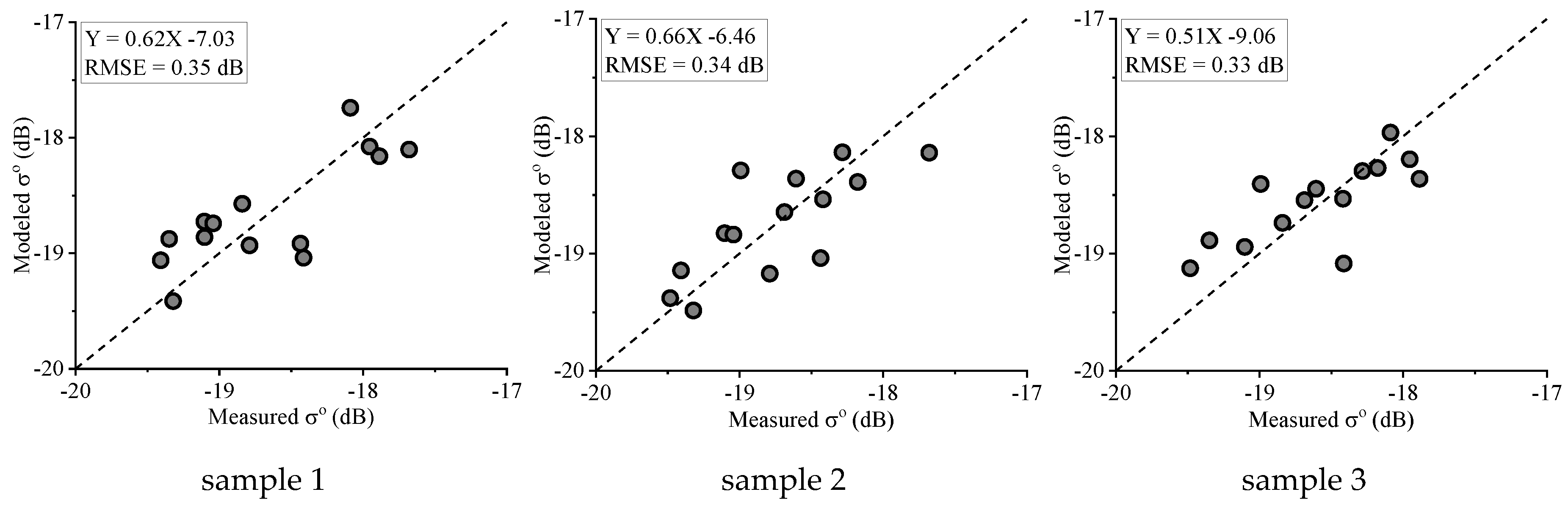
Figure 10.
Scatterplots between estimated and measured FMC.
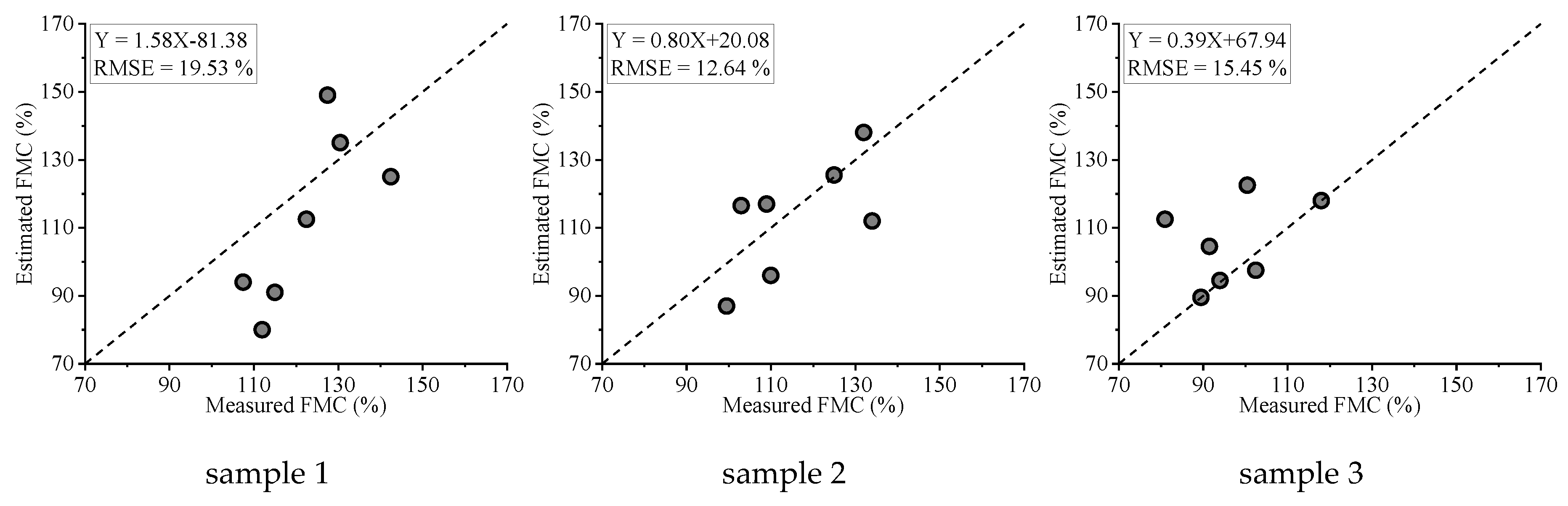
Figure 11.
The time-series distribution of estimated and measured FMC.

Figure 12.
Scatterplots of training and testing results from Landsat 8 OLI data.
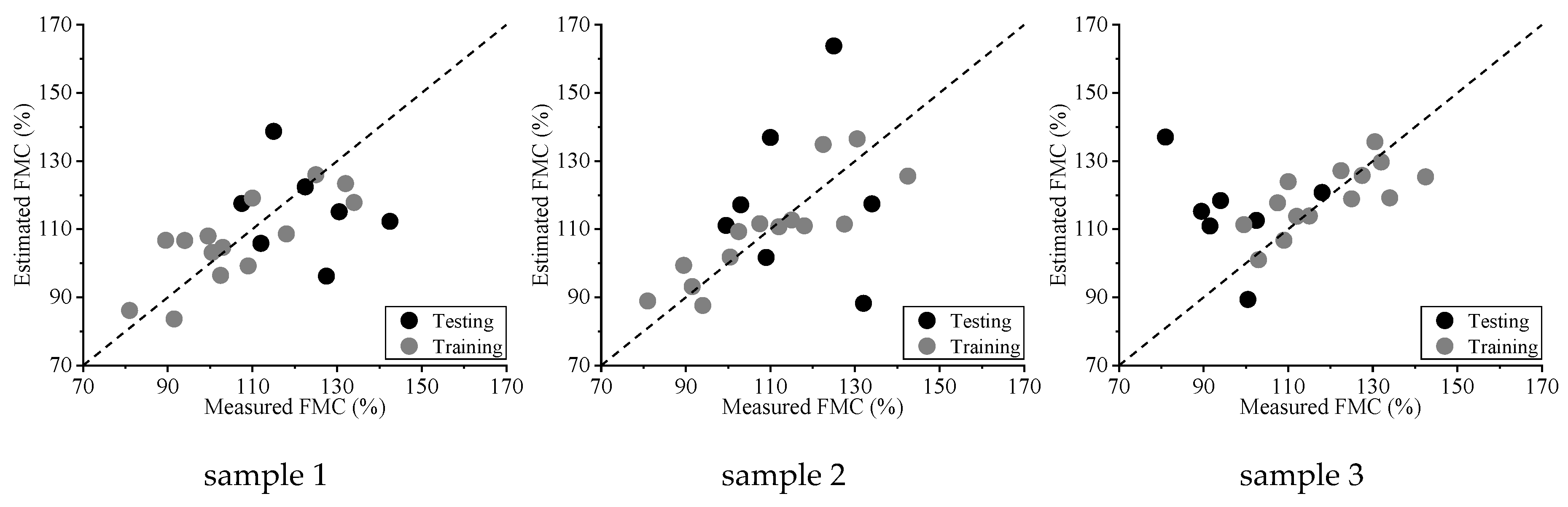
Figure 13.
The time-series trend of estimated and measured FMC.
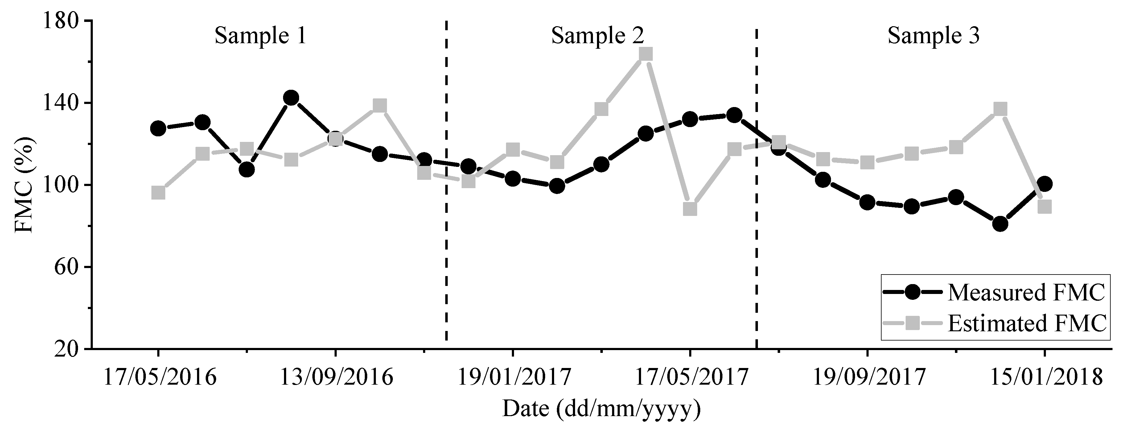
Table 1.
Root mean square error (RMSE) between measured and estimated FMC.
| Samples | Training | Testing | All |
|---|---|---|---|
| sample 1 | 9.52% | 20.11% | 13.97% |
| sample 2 | 8.69% | 26.21% | 16.71% |
| sample 3 | 8.69% | 26.73% | 16.99% |
© 2019 by the authors. Licensee MDPI, Basel, Switzerland. This article is an open access article distributed under the terms and conditions of the Creative Commons Attribution (CC BY) license (http://creativecommons.org/licenses/by/4.0/).
Share and Cite
MDPI and ACS Style
Wang, L.; Quan, X.; He, B.; Yebra, M.; Xing, M.; Liu, X. Assessment of the Dual Polarimetric Sentinel-1A Data for Forest Fuel Moisture Content Estimation. Remote Sens. 2019, 11, 1568. https://0-doi-org.brum.beds.ac.uk/10.3390/rs11131568
AMA Style
Wang L, Quan X, He B, Yebra M, Xing M, Liu X. Assessment of the Dual Polarimetric Sentinel-1A Data for Forest Fuel Moisture Content Estimation. Remote Sensing. 2019; 11(13):1568. https://0-doi-org.brum.beds.ac.uk/10.3390/rs11131568
Chicago/Turabian StyleWang, Long, Xingwen Quan, Binbin He, Marta Yebra, Minfeng Xing, and Xiangzhuo Liu. 2019. "Assessment of the Dual Polarimetric Sentinel-1A Data for Forest Fuel Moisture Content Estimation" Remote Sensing 11, no. 13: 1568. https://0-doi-org.brum.beds.ac.uk/10.3390/rs11131568
Note that from the first issue of 2016, this journal uses article numbers instead of page numbers. See further details here.