Clustering of Wall Geometry from Unstructured Point Clouds Using Conditional Random Fields


Department of Civil Engineering, TC Construction—Geomatics, KU Leuven—Faculty of Engineering Technology, 9000 Ghent, Belgium
*
Author to whom correspondence should be addressed.
Remote Sens. 2019, 11(13), 1586; https://0-doi-org.brum.beds.ac.uk/10.3390/rs11131586
Submission received: 14 May 2019
/
Revised: 11 June 2019
/
Accepted: 12 June 2019
/
Published: 4 July 2019
(This article belongs to the Special Issue Heritage 3D Modeling from Remote Sensing Data)
Abstract
:The automated reconstruction of Building Information Modeling (BIM) objects from point cloud data is still subject of ongoing research. A vital step in the process is identifying the observations for each wall object. Given a set of segmented and classified point clouds, the labeled segments should be clustered according to their respective objects. The current processes to perform this task are sensitive to noise, occlusions, and the associativity between faces of neighboring objects. The proper retrieval of the observed geometry is especially important for wall geometry as it forms the basis for further BIM reconstruction. In this work, a method is presented to automatically group wall segments derived from point clouds according to the proper walls of a building. More specifically, a Conditional Random Field is employed that evaluates the context of each wall segment in order to determine which wall it belongs to. First, a set of classified planar primitives is obtained through algorithms developed in prior work. Next, both local and contextual features are extracted based on the nearest neighbors and a number of seeds that are heuristically determined. The final wall clusters are then computed by decoding the graph. The method is tested on our own data as well as the 2D-3D-Semantics (2D-3D-S) benchmark data of Stanford. Compared to a conventional region growing method, the proposed method reduces the rate of false positives, resulting in better wall clusters. Overall, the method computes a more balanced clustering of the observations. A key advantage of the proposed method is its capability to deal with wall geometry in complex configurations in multi-storey buildings opposed to the presented methods in current literature.
1. Introduction
The production of as-built Building Information Modeling (BIM) models is becoming increasingly widespread in the Architectural, Engineering and Construction (AEC) industry. These models reflect the state of the building up to as-built conditions and are used for quality control, quantity take-offs, maintenance, and project planning [1,2]. The geometry of an as-built BIM is obtained by creating a model from scratch based on measurements on site or updating an existing as-design model. The emphasis of this work is on the reverse engineering of as-built BIMs without a prior model since few buildings have a model. Currently, the objects involved are created manually by creating geometry representations based on point cloud data captured of the built structure. It is a cumbersome procedure which requires significant time investment and trained personnel. We specifically target the geometry of wall objects as they form the basis of the structure and can be reliably identified in point cloud data. This work is the fully integrated extension of the prototype presented in previous work [3]. The method was expanded to operate on large scale datasets and includes additional functionalities to cope with the shortcomings of the initial prototype.
The reconstruction of wall geometry from point cloud data is typically considered as an unsupervised process. However, the interpretation of this data is sensitive to noise, clutter and the complexity of the structure. Also, the amount of data introduces significant computational challenges [4]. The acquisition of point cloud data is typically performed by remote sensing techniques which are bound to Line-of-Sight (LoS). The resulting datasets are therefore inherently occluded in inaccessible areas and isolated spaces such as the areas above ceilings. Reasoning algorithms make assumptions about these zones which are prone to misinterpretation. This issue is often mitigated by integrating the sensor’s position and orientation. However, as it is our goal to operate on sensor independent point cloud data, we consider the inputs as unstructured. Also, we limit the scope of the procedure to the clustering of wall observations since many other classes can be automatically derived from their geometry e.g., doors, windows, floors and ceilings. The clustering is performed on object level based on both simplistic and complex BIM wall representations. We deal with wall observations which are not parallel to the main wall faces and are located in highly cluttered and noisy environments. Also, our approach can deal with complex wall configurations such as near-coplanar wall faces of different walls by simultaneously computing the wall labels for every segment. Similarly, we process the entire structure simultaneously since our method is capable of dealing with multi-storey observations.
2. Background and Related Work
The reconstruction of BIM entities from point cloud data is a popular subject. Several procedures are discussed that target the reverse engineering of wall geometry from geometric inputs. The proposed unsupervised methods typically consist of the following set of consecutive algorithms [5]. First, a preprocessing of the geometric inputs is performed to increase the computational efficiency. In 2D methods, the point cloud is typically restructured as a number of raster images, each representing a section of the data or projected information [6,7]. In 3D methods, the point cloud is often represented in a voxel octree which significantly enhance nearest neighborhood searches [8] (Figure 1a). Following the preprocessing, the data is segmented into groups based on the associativity of the point characteristics. Algorithms such as RANSAC asses properties e.g., normals or colors and combine the points into regions with similar attributes. Alternative methods use region growing, Probabilistic Graphical Models, and so on [9,10]. Once a set of regions is established, the geometry of the regions are often replaced by primitives to reduce the data. Typically, lines are employed in 2D procedures and planes or other primitives are used in 3D methods [8,11,12,13]. The resulting segments are then classified into a number of preset outputs. In building reconstruction, the classes typically consists of a buildings’ common components such as floors, ceilings, walls and so on. A set of local and contextual features (Figure 1b) are extracted from each observation after which its class is determined by feeding the features into a decision function. The functions involved can be based on heuristics or machine learning [14,15,16]. Several researchers combined man made rules in a decision function to classify 3D geometry inputs [16,17,18]. While being very efficient, heuristics are typically case specific as the model weights and parameters are intuitively determined. More flexible methods employ machine learning procedures to deal with the wide variety of object parameters, classes, and observations. Xiong et al. [15,19] extract features from presegmented meshes and classify them using stacked learning. Markov random fields (MRF) and conditional random fields (CRF) are also proposed for the classification of building geometry [20,21,22]. A popular approach is the use of convolutional neural networks (CNN) that recombine sets of neurons in different layers in order to process a set of input vectors to a known set of outputs [23]. Especially for 2D inputs, inference accuracies of over 90% are reported for the detection of building objects on databases such as CMP [24], eTRIMS [25], and ECP [26]. The resulting labeled wall segments serve as input to the wall clustering that is the emphasis of this work. A similar reasoning, as in segmentation and classification, is employed to identify a set of clusters that each contain all the relevant observations of a wall that conform to the BIM model (Figure 1c). Finally, these groups serve as input for the application specific reconstruction algorithms. Depending on the application, different geometry definitions are considered for the walls. For instance, walls can be considered as volumetric wall entities (BIM) or surface based geometry where each wall face is a separate entity (CityGML) [27]. Some applications even consider walls as a child entity of room geometry [28].
The paradigm of clustering observations according to their wall representations is a common step in BIM reconstruction procedures. Similar to segmentation and classification, the methods involved range from heuristics to region growing, model based methods, graphs, and machine learning techniques [5]. The majority of methods consider simplistic box definitions for the wall geometry representation i.e., walls are considered an aggregate of coplanar and parallel segments.
For methods that are only concerned with the reconstruction of wall faces, the clustering problem is typically reduced to the detection of the predominant plane [29]. For instance, Oesau et al. [17] rely on the collinearity of the segments of a wall face. They implement a Hough transform to retrieve all the points on a wall face in a 2D slice of the point cloud. Adan et al. [30] present a similar method that represents the point cloud in a 2D histogram along its zenith. Similar results are presented by Previtali et al. [31], Budroni et al. [32], Valero et al. [33], and Nikoohemat et al. [16]. 3D methods are also considered. For instance, Thomson et al. [34] implement a Point Cloud Library (PCL) based RANSAC method that extracts the main planar faces in a point cloud structure. They subdivide the output clusters based on the euclidean distance between the boundaries of the segments in order to separate coplanar walls. Overall, these methods are promising in scenes that have limited wall detailing and where complex wall configurations are not an issue.
The researchers that do actually cluster both sides of walls typically do so conform a box or rectangle. A promising method is presented by Mura et al. Mura et al. [29] that project their detected wall segments onto a 2D plane and cluster them based on coplanarity and collinearity. They first compute a directional clustering which yields the main orientation of the individual walls. For each direction, a 1D mean-shift clustering [35] is performed which identifies all possible offsets of parallel wall segments of that orientation. Finally, they compute a representative line for each wall cluster in 2D that is then used in the reconstruction step. Ochmann et al. [36] on the other hand use heuristics to cluster parallel and coplanar wall segments. Each potential pair of wall surface lines fulfilling certain constraints is considered as the two opposite surfaces of a wall separating adjacent rooms. The segments are then clustered by evaluating the overlap and the orientation of the candidates. Aside from heuristics, model based methods are also used. Recent variants of the RANSAC algorithm [37] are extended to not just fit simplistic models such as lines or planes but match entire walls. For instance, Oesau et al. [17] employ a two-line hypothesis created by RANSAC to detect corner configurations for their walls. Similar to the single faced clustering, the majority does not consider the grouping of more complex wall geometry or highly associative walls.
There are currently few methods that cluster wall segments into more complex walls. These walls represent their actual geometry which includes wall detailing such as observations of niches, protrusions, and openings. They consist of segments with varying normals and sizes in complex configurations. However, there are several methods that target different clustering tasks that might be extended to the clustering of wall geometry. For instance, Ikehata et al. [38] exploit k-medoids and heuristic segment clustering to cluster room observations. They project the observations of the rooms in a raster image and use the 2D representation to initialize a selective seeding algorithm to determine to determine which room an observation belongs too. Armeni et al. [39,40] consider the idea of employing connected component graphs. Prior to the clustering of their observations, they subdivide their graph by removing invalid edges give some validation criterion e.g., the distance between the boundaries. As a result, some parts of the graph become isolated with only segments connecting to segments within the part. These connected components have a significantly lower combination complexity and also are less prone to misclustering since not every possible edge is considered. Armeni et al. use this method in combination with region growing to cluster room segments. They observe the wall density signature along the length of the edge in order to detect whether or not the edge collides with a wall (peak). Connected components are also used to cluster of roof objects. He et al. [41] considers connected component graphs as aggregates of roof structures to detect all the roof observations belonging to a single building. The concept of component graphs is a promising technique which we also use for the complex wall clustering. Both heuristics and machine learning algorithms can be used to dispatch invalid edges from the graph after which the remaining linked observations can be subjected to a subsequent clustering. For instance, Gilani et al. [42] use connected component graphs to merge line segments of roof edges in aerial lidar applications. Alternatively, Mura et al. [43] use of structural paths for room segment clustering. They propose region growing in an adjacency matrix based on pairwise relations between the observations. Given the connectivity of the graph structure, they iteratively asses the edges for one of k predefined connections. As a result, their method computes sets of patches enclosing a target space based on a seed node. In our research, we opt for the use of machine learning techniques in connected component graphs to simultaneous assign the state of all the observed segments which is expected to yield a more balanced clustering than the one-sided stopping criteria of, for instance, region growing.
A powerful machine learning method for the simultaneous segmentation and clustering are conditional random fields (CRFs) [44]. Given a graph which consists of a set of nodes and edges, a best fit configuration can be computed by decoding the network. It is considered an instance of supervised pattern recognition where a set of states is assigned to a fixed number of observations. Several methods exist do compute decoding or inference of a CRF, most of which are approximate since the dependencies of most graphs are intractable. For instance, there are variants of the Iterated Conditional Mode (ICM) algorithm, graph cuts [28,45,46] and loopy belief propagation [6,13,47]. As this technique requires the exact number of states or walls to be known prior to the feature extraction, it is paramount to perform a proper seeding in the graph. This can be challenging since not all walls have stereotypical seeds. Also, the estimation of the model parameters when factorizing the graph is sensitive to outliers and requires robust features and training data. Despite these shortcomings, we believe CRF is a promising approach since allows the integration of both unary and pairwise relations which aids the clustering in complex wall configurations.
3. Methodology
This section contains the detailed description of the present clustering method. The goal is to group the segmented and classified wall observations into the minimum number of relevant walls that occur in a generic structure. The procedure is feedforward and can be divided into modular steps. First, a presegmentation is conducted along with a classification step based on prior work [48]. Following, a set of connected component graphs are extracted from a graph structure of the observations based on edge criteria. Next, a set of seeds is extracted by running a fast heuristic region growing method on the graphs. These seeds form the basis of the walls of the building. In the final stage, each observation is assigned to one of the walls given unary and pairwise features. The entire pipeline builds upon the UGM toolbox [49] in Matlab and the pipeline is integrated in the Rhinoceros Grasshopper which is used as the user platform. Each step is discussed in detail in the paragraphs below.
3.1. Data Preprocessing
The segmentation and classification aim to reduce the data and isolate the wall observations. First, a voxel octree is constructed from the unstructured point cloud to increase its efficiency. The segmentation is performed by an efficient region growing algorithm that identifies planar regions in the point cloud [50]. These regions are replaced by planar mesh geometry after which they are classified as part of common building components. 6 categories are considered including floors, ceilings, roofs, walls, beams and clutter. Each observed segment is assigned to a class employing a pre-trained Random Forests classification model [48]. Given the class labels of the segments, the observations of wall geometry are isolated and the remainder of the surfaces is used in the clustering step to provide context for the decision functions involved.
3.2. Connected Component Graph Creation
The assignment of the wall segments is a noise sensitive procedure. This is especially true in our method where we look to simultaneously assign thousands of segments to potentially hundreds of walls. As the number of potential walls grows, so does the confusion in the state estimation and the computational complexity. However, not every combination is to be evaluated. The presented method relies on connected component graphs as an initial segmentation of the wall observations. First, a densely connected graph is constructed where each node is a wall observation and E is a set of edges that connect neighboring segments (Figure 2a). The graph structure is represented in an adjacency matrix where each node is connected to its k nearest neighbors based on the euclidean distance between the wall segment’s boundaries. The connected components, which are isolated subgraphs of G, are retrieved by removing unlikely or unwanted edges from the graph. In this research, a set of heuristic rules is applied to validate the edges in the graph. An edge is conditioned to comply with one of three distance criteria (Equation (1)). The first criterion is that the absolute distance between boundaries should not exceed . This hard constraint should be set fairly strict (<1 m) since it can connect any two observations which rapidly increases computational complexity and also links observations that are not meant to influence each other e.g., surfaces on both sides of an alley. The second and third criterion respectively are the distance between coplanar segments and the distance between parallel segments given the overlap between and with the projected geometry of onto along (Figure 2b). These are more conventional constraints and can be more lax (<2 or 3 m) since they rely on the box definition of the observations.
In addition to the three distance criteria, the edges should also not intersect with any other building geometry. This includes other wall segments and basic room information. The ceilings that directly overlay any floors are extruded downwards and used to create a 3D convex hull that roughly represent the buildings’ rooms (Figure 2c). The convex hull is shrank with an offset of 0.1 m to avoid wall segments adjacent to floor or ceiling segments to fall within its geometry. Edges that collide with either other wall segments or room geometry are removed from the graph. Also, the potential thickness of connected wall segments is evaluated. Given both segments and at the ends of the edge , a bounding box is computed in the plane of the largest wall segment. The thickness of this bounding box is evaluated to determine whether an edge is valid. The hypothesis is that if this distance exceeds a certain threshold e.g., 1 m, the wall segments are highly unlikely to belong to the same wall. The result of the removal of edges from the graph is a set connected component graphs where segments only are connected with other segments within the component (Figure 2e).
3.3. Clustering
In this work, the clustering paradigm is considered a classification task that can be solved with supervised pattern recognition techniques. More specifically, we propose the use of conditional random fields (CRF) as discussed in the related work. A major advantage of this technique is that every seed is evaluated simultaneously so that the clustering is not dependent on heuristic stopping criteria as is the case with conventional methods. This is expected to result in a more balanced clustering where each s is assigned to the best fit c instead of the cluster with the largest seed. The objective is to find the most optimal labeling of the set of nodes s that can take one of states. This is performed by computing the a posteriori probability distribution of the states over the nodes in the graph. In order to do so, the graph is restructured as a factor graph (Figure 3). Depending on the number of output clusters in the component graph, a set of unary and pairwise potentials is established for each node and edge. The set of edges in the network is given non-negative weights along with a set of feature vectors. Additionally, we replace the nodes that function as the seeds by terminal nodes similar to the graph structure used in graph cuts [51]. These nodes t take one of u fixed states since they serve as seeds. The labeling is performed by maximizing the probability over the network. Each of the above steps, including the seeding for the number of outputs, the edge potential initialization and the labeling are discussed in the paragraphs below.
3.3.1. Seeding
It is stated that while the clustering of region growing itself is likely to be erroneous, at least a part of each wall is represented in a cluster. Therefore, we used the largest segment in each initial cluster as the seeds for the graph. The region growing algorithm operates as follows. Iteratively, the neighbors of are evaluated. Starting from the largest neighbor, a bounding box criterion similar to the initial graph definition is evaluated. However, instead of computing the bounding box of only and , all the s in the current c are evaluated along the average weighted by the percentual surface areas of . Given this bounding box, is merged with the cluster if the total bounding box thickness does not exceed . This hard constraint allows for flexible growing but restricts the cluster from becoming too large. If no more members can be added to the cluster, the next largest unclustered segment is selected as a new seed and the process is repeated for the remaining surfaces. Additionally, the clusters are conditioned to have more than one surface or that the surface area is sufficiently large. This avoids singular surfaces that do not fit well with other segments to result in erroneous walls. The result is a set of clusters , with each c representing the available observations of a single wall. The nodes corresponding to the seeding segments are given a fixed state and will serve as the basis for the feature extraction in the CRF.
3.3.2. Potential Computation
The potentials are initialized for each edge and node s in the graph based on their respective feature vectors (Figure 4a). We define both pairwise and unary potentials to determine which cluster a node belongs to. The pairwise potentials are computed given a set of edge features and corresponding weights . Associative values are computed for the euclidean distance between the boundaries of and and the potential bounding box thickness according to the largest segment of the two neighbors. We use exponential functions to model the information to ensure non-negative associative features.
The unary potentials are initialized based on the affinity of a node to a certain cluster represented by each of the seed nodes . A set of features and corresponding weights are defined. In this work, two features are defined for each seed. The features include the thickness of the bounding box of and and the absolute distance between the boundaries of and .
3.3.3. Probability Estimation
The a posteriori probability distribution of the conditional random field is found by factorizing the graph (Figure 4b). We define the conditional probability of the states in the network as follows (Equation (2)).
where is the normalizing partitioning function, describes the unary potentials of the nodes with relation to the seed nodes, and describes the pairwise potentials between neighboring nodes. The graph is decoded by maximizing the conditional probability. However, exact decoding is unfeasible in a densely connected CRF. Therefore, we approximate the decoding using a generalized iterated conditional mode algorithm as implemented by Schmidt [49]. After computing the most likely configuration of the graph, the segments are clustered according to the labels. The result is a set of clustered wall segments.
4. Experiments
Two test cases are presented to evaluate the algorithm’s performance. The first experiment is a small scale test on a multi-storey school building on our technology campus in Ghent, Belgium (Figure 5a). The second test case is the 2D-3D-Semantics (2D-3D-S) benchmark data of Stanford [40] which consists of 6 indoor areas (Figure 5b). Both experiments vary in scale, the presence of interior and exterior walls and multiple floors. Furthermore, the first dataset is evaluated through cross-validation while the second data set was purely used for testing with the same parameters. Both experiments were tested against a conventional region growing method. The region growing method is based on our segmentation method presented in previous work [50] and solely uses the bounding box criterion to determine which edges are valid. Both methods use similar settings to evaluate the extent for which CRF can enhance clustering results. The results of both experiments are discussed in the following paragraphs.
4.1. Experiment 1: Technology Campus
The school facility on the technology campus in Ghent is a four-storey structure with a variety of rooms including a laboratory, two classrooms, a staircase, and a maintenance room (Figure 5). A large amount of clutter is present in the environment. The structure’s interior and exterior was acquired with Terrestrial laser scanning. A total of 53 scans were conducted resulting in a highly accurate and dense dataset of over 500 million points. Nearly 7000 surfaces were detected by the preprocessing, 258 of which represent wall observations. The mesh generated on the point cloud had an average standard deviation 0.001 m. A total of 14 multi-storey walls were defined for the testing. connections were evaluated for each s. The following parameters were used for the region growing. The bounding box thickness was set to 0.8 m, the absolute distance between boundaries m, the coplanar distance m, the coplanar boundary distance m, and the distance between overlapping parallel s is equal to . In total, 7 connected components were detected in s of which 6 components consisted of a single surface. In the validation step, 6 of the 7 components complied with the thickness criterion and thus were isolated.
The 216 segments within the remaining connected component graph were processed by the proposed conditional random fields method. For the state estimation, the seeds are used that were extracted from the region growing. A total of 7 valid seeds were detected. As unary potentials, the bounding box thickness, and edge length were computed between the observations and each seed segment. The pairwise potentials are initialized based on the same features but between neighboring segments. The weights of the features was set equally over all states as there should not be bias over which cluster an observation belongs to. The parameters for the different features were learned through 5-fold cross-validation. Iteratively, 80% of the dataset was used to train the parameters while 20% was used for testing. The final model parameters were established by averaging the results. While the training data set is fairly small, only a small number of parameters is to be trained ( for the unary potentials and for the pairwise potentials). The decoding was performed using a generalized iterated conditional mode algorithm as implemented by Schmidt [49]. of the segments were properly clustered in less than 1 s. Together with the initial valid connected components, of the wall geometry was assigned to the proper cluster. This is promising given the complexity of the structure and the variety of the geometry. However, some errors still remain. Especially smaller segments are error prone due to their high associativity with multiple seeds.
For the validation, the results of the CRF method are compared to the results of a conventional region growing algorithm that was used to establish the seeds. Both methods operate with the same parameters and features. As discussed above, the main difference between these methods is the simultaneous assignment of the segments with the CRF in contrast to the one-sided stopping criteria of the region growing. As an example, the results of two highly associative walls are discussed (Figure 6). These walls are near coplanar with several segments of surrounding , have different thicknesses at different heights, and have protrusions, niches and recesses. This is considered as a worst case scenario where even experienced modelers would struggle to assign the segments to the proper clusters.
As discussed above, the region growing method prioritizes segments with a large surface area. Therefore, the algorithm iterates through the segments and evaluates the observations with respect to . As expected, the majority of the segments comply with the validation criteria based on . The remainder of the segments is assigned to leading to a severely unbalanced clustering. In the CRF method, the features between neighbors and with respect to and are evaluated simultaneously leading to a more proper clustering. It is observed that while the results of the CRF are far from perfect, it provides a significantly better clustering than the conventional region growing.
4.2. Experiment 2: 2D-3D-Semantics Stanford
The 2D-3D-S dataset contains both 2D, 2.5D, and 3D observations of 6 large-scale indoor areas of 3 different buildings of mainly educational and office use (Figure 5c). It covers over 6000 m2 of preannotated meshes and point clouds. To establish the ground truth, the segments classified as wall geometry were manually grouped per volumetric wall instance. In total, over 1552 wall observations were clustered into 448 walls. While numerous walls only consist of parallel surfaces, more complex wall geometry is also present. As previously stated, all areas were used for testing, using the same parameters learned from the first experiment. The feature extraction was also performed with the same parameters as in the first experiment, as was the region growing.
The results of the experiment are shown in Table 1 and Table 2, and Figure 7 and Figure 8. Overall, each dataset consisting of hundreds of observations was processed in a matter of seconds due to the preprocessing of the initial dataset of nearly 700 million points. On average, the processing of 250 wall segments took 5.5 s for the graph creation, feature extraction, initial region growing, and optimization through CRF. The fast processing time is due to the sparsity of the graph as shown in Figure 5. Each surface on average is connected to 3 other surfaces which is expected due to the laxity of the edge criteria. Overall, the results for the presented method are promising. On average, 90.6% of the walls were found with an average precision of 86.1% compared to the region growing where respectively 85.0% and 83.3% are observed. This is largely due to the simplicity of most of the scenery such as parallel walls (Figure 7). However, the real test results are located in the evaluation of the complex wall geometry. Figure 8 shows several cases of complex wall segment configurations. It can be clearly observed that the region growing, due to the edge criteria transitivity, is clustering these scenarios and is inherently erroneous. In the presented method, where the seeds are evaluated simultaneously, there is a more balanced clustering. Not only does this affect the clustering of the walls but it also heavily influences the future reconstruction of the entities that are more logically distributed by the proposed method. Overall, it is stated that the CRF method shows promising results for clustering wall geometry from different sources in an efficient manner. The results of the experiments are shared at the following url: https://osf.io/b7vqe/ As the algorithm is embedded in the Rhinoceros software, the files are native Rhino 6.3 dm files. Each file includes the geometry as imported from the 2D-3D-S database along with the proper annotations. Additionally, extra layers have been created for the ground truth (wallclusters), the results of the region growing (wallregiongrowing), and the results of the proposed CRF method (wallCRF). The names of the walls are unordered ranging from 1 to the maximum number of walls.
Despite the promising results, several shortcomings are still present in the proposed method. For instance, the seeding is still dependent on initial region growing. As this method is inherently flawed, some errors will serve as input to the CRF. As the CRF does not discriminate between the input seeds, an error in the seeding will have a significant effect on the CRF clustering. This is both true for undersegmented walls (too few clusters) as for oversegmented walls (too many clusters) that are treated equally by the CRF. Another shortcoming might be the sparsity of the connected components. The number of potential edges is significantly restricted by several heuristic edge criteria. While this proves efficient, too strict criteria will result in too sparse connected components which in turn will result in oversegmentation. However, the current criteria are reasonably lax and a sparse network also prevents odd clustering results that are common for probabilistic methods.
5. Discussion
The objective of clustering wall geometry is retrieving a sufficient number of wall observations for each wall so BIM Wall objects can be modeled from them. The target entities are parametric volumetric BIM objects and thus the walls should be clustered according to this representation. Depending on the model, different types of clustering are required. For instance, CityGML [27] has a surface based wall representation and Oesau et al. [17] focus on room based reconstruction. We believe our method can also be extended towards other clustering tasks since the simultaneous assignment of wall or room labels allows for better informed decisions compared to one-sided decision functions such as region growing.
The paradigm of wall clustering is affected by a number of parameters. The following two parameters should be taken into consideration when clustering wall observations. First, the success of every method heavily relies on the correspondence of the model parameters to the observations of a real structure. For instance, observations of simplistic walls will be clustered properly by most methods since the abstract box definition applies to the majority of the observations. As the wall definitions become more complex to match the real situation, the parameters become increasingly diverse and more difficult to predict up to the point that human operators can also no longer appropriately cluster the data. It is stated that one-sided methods can only reliably cluster abstract walls while simultaneous assignment methods like ours are also suited to deal with complex wall geometry. Secondly, each process is subject to noise and outliers. In the subsequent processes of acquisition, segmentation, classification, and clustering, there is an accumulation of errors that will affect the final grouping of the observations. Each process should therefore be flexible enough to deal with the outliers from previous methods. This is more challenging for heuristic methods since random noise is hard to define with strict rules. Weighted decision functions can be more easily extended to accommodate these occurrences.
Several improvements can be considered for our workflow. For instance, the presented method is data driven as is the state-of-the-art in wall clustering. Currently, solely geometric features are computed for the seed estimation and subsequent clustering. There is the opportunity to integrate color or sensor information to enhance the clustering results. However, both offer only limited added value towards the retrieval of highly occluded multi-room walls. Another method is to learn not from manually labeled wall segments but from actual BIM models. Given the individual surfaces of the walls of a BIM model, geometric features, and model parameters can be learned from preexisting BIMs. However, not every BIM is modeled using the same convention, and could result in confusing parameters sets preferring single-storey walls over multi-storey walls depending on the training data set.
6. Conclusions
In this work, an unsupervised method is presented to cluster wall geometry from unstructured point clouds of buildings. The goal is to group the wall observations per wall object which will form the basis for a BIM reconstruction. A novel 3D approach is proposed that computes the best fit assignment of the wall observations to the different walls. Prior to the clustering, the data is preprocessed by a segmentation and classification framework which drastically reduces the data and to increase the amount of information of each observed segment. The resulting classified wall segments are then processed by our clustering algorithm which is based on Conditional Random Fields. A graph is constructed connecting each segment to its nearest neighbors. The connectivity of the graph is evaluated and invalid edges are removed resulting in a set of connected component graphs. Within these subgraphs, each of the observations is assigned to one of the walls based on both unary and pairwise features. The state estimation is initialized with region growing and the final clustering is performed through decoding the factorized graph. The result is a set of clustered segments that correspond to the wall objects in a building.
The algorithm was tested on our own data and the 2D-3D-Semantics (2D-3D-S) benchmark data of Stanford. The experiments reported promising results with over 90% recall for the clustering of the wall segments of the Stanford dataset. When compared to a conventional region growing method, it was shown that the presented approach resulted in a more balanced clustering. Despite the high recall and precision, some errors still remain. Especially in highly complex wall configurations with associative faces of multiple walls there was significant confusion about which cluster a segment belonged to. The future work will deal with these shortcomings by implementing additional features. Overall, the method presents an alternative approach to one sided clustering algorithms such as region growing.
Author Contributions
M.B. conceived the work and was supervised by M.V.
Funding
This research was funded by the European Research Council (ERC) under the European Union’s Horizon 2020 research and innovation programme (grant agreement 779962) and the Geomatics research group of the Department of Civil Engineering, TC Construction at the KU Leuven in Belgium.
Conflicts of Interest
The authors declare no conflict of interest.
References
- Volk, R.; Stengel, J.; Schultmann, F. Building Information Modeling (BIM) for existing buildings—Literature review and future needs. Autom. Constr. 2014, 38, 109–127. [Google Scholar] [CrossRef]
- Patraucean, V.; Armeni, I.; Nahangi, M.; Yeung, J.; Brilakis, I.; Haas, C. State of research in automatic as-built modelling. Adv. Eng. Inform. 2015, 29, 162–171. [Google Scholar] [CrossRef] [Green Version]
- Bassier, M.; Vergauwen, M. Clustering of wall geometry from unstructured point clouds. Int. Arch. Photogramm. Remote Sens. Spat. Inf. Sci. 2019, XLII-2/W9, 101–108. [Google Scholar] [CrossRef]
- Tang, P.; Huber, D.; Akinci, B.; Lipman, R.; Lytle, A. Automatic reconstruction of as-built building information models from laser-scanned point clouds: A review of related techniques. Autom. Constr. 2010, 19, 829–843. [Google Scholar] [CrossRef]
- Nguyen, A.; Le, B. 3D point cloud segmentation: A survey 3D. In Proceedings of the 6th IEEE Conference on Robotics, Automation and Mechatronics (RAM), Manila, Philippines, 12–15 November 2013; pp. 225–230. [Google Scholar] [CrossRef]
- Landrieu, L.; Mallet, C.; Weinmann, M. Comparison of belief propagation and graph-cut approaches for contextual classification of 3D lidar point cloud data. In Proceedings of the IEEE International Geoscience and Remote Sensing Symposium (IGARSS), Fort Worth, TX, USA, 23–28 July 2017. [Google Scholar]
- Anagnostopoulos, I.; Patraucean, V.; Brilakis, I.; Vela, P. Detection of walls, floors and ceilings in point cloud data. In Proceedings of the Construction Research Congress 2016, San Juan, Puerto Rico, 31 May–2 June 2016. [Google Scholar]
- Vo, A.V.; Truong-Hong, L.; Laefer, D.F.; Bertolotto, M. Octree-based region growing for point cloud segmentation. ISPRS J. Photogramm. Remote Sens. 2015, 104, 88–100. [Google Scholar] [CrossRef]
- Dimitrov, A.; Golparvar-Fard, M. Segmentation of building point cloud models including detailed architectural/structural features and MEP systems. Autom. Constr. 2015, 51, 32–45. [Google Scholar] [CrossRef]
- Barnea, S.; Filin, S. Segmentation of terrestrial laser scanning data using geometry and image information. ISPRS J. Photogramm. Remote Sens. 2013, 76, 33–48. [Google Scholar] [CrossRef]
- Lin, Y.; Wang, C.; Cheng, J.; Chen, B.; Jia, F.; Chen, Z.; Li, J. Line segment extraction for large scale unorganized point clouds. ISPRS J. Photogramm. Remote Sens. 2015, 102, 172–183. [Google Scholar] [CrossRef]
- Fan, Y.; Wang, M.; Geng, N.; He, D.; Chang, J.; Zhang, J.J. A self-adaptive segmentation method for a point cloud. Vis. Comput. 2018, 34, 659–673. [Google Scholar] [CrossRef]
- Vosselman, G.; Rottensteiner, F. Contextual segment-based classification of airborne laser scanner data. ISPRS J. Photogramm. Remote Sens. 2017, 128, 354–371. [Google Scholar] [CrossRef]
- Bassier, M.; Vergauwen, M.; Van Genechten, B. Automated semantic labelling of 3D vector models for Scan-to-BIM. In Proceedings of the 4th Annual International Conference on Architecture and Civil Engineering (ACE 2016), Singapore, 25–26 April 2016; pp. 93–100. [Google Scholar] [CrossRef]
- Xiong, X.; Adan, A.; Akinci, B.; Huber, D. Automatic creation of semantically rich 3D building models from laser scanner data. Autom. Constr. 2013, 31, 325–337. [Google Scholar] [CrossRef] [Green Version]
- Nikoohemat, S.; Peter, M.; Oude Elberink, S.; Vosselman, G. Exploiting Indoor Mobile Laser Scanner Trajectories for Semantic Interpretation of Point Clouds. ISPRS Ann. Photogramm. Remote Sens. Spat. Inf. Sci. 2017, IV-2/W4, 355–362. [Google Scholar] [CrossRef]
- Oesau, S.; Lafarge, F.; Alliez, P. Indoor scene reconstruction using feature sensitive primitive extraction and graph-cut. ISPRS J. Photogramm. Remote Sens. 2014, 90, 68–82. [Google Scholar] [CrossRef] [Green Version]
- Jung, J.; Hong, S.S.; Jeong, S.; Kim, S.; Cho, H.; Hong, S.S.; Heo, J. Productive modeling for development of as-built BIM of existing indoor structures. Autom. Constr. 2014, 42, 68–77. [Google Scholar] [CrossRef]
- Xiong, X.; Huber, D. Using Context to Create Semantic 3D Models of Indoor Environments. In Proceedings of the British Machine Vision Conference 2010, Aberystwyth, UK, 30 August–2 September 2010; pp. 45.1–45.11. [Google Scholar] [CrossRef]
- Anand, A.; Koppula, H.S.; Joachims, T.; Saxena, A. Contextually Guided Semantic Labeling and Search for 3D Point Clouds. Int. J. Robot. Res. 2012, 32, 19–34. [Google Scholar] [CrossRef]
- Wolf, D.; Prankl, J.; Vincze, M. Fast semantic segmentation of 3D point clouds using a dense CRF with learned parameters. In Proceedings of the IEEE International Conference on Robotics and Automation (ICRA), Seattle, WA, USA, 26–30 May 2015. [Google Scholar]
- Niemeyer, J.; Rottensteiner, F.; Soergel, U. Contextual classification of lidar data and building object detection in urban areas. ISPRS J. Photogramm. Remote Sens. 2014, 87, 152–165. [Google Scholar] [CrossRef]
- Lotte, R.; Haala, N.; Karpina, M.; Aragao, L.; Shimabukuro, Y. 3D Façade Labeling over Complex Scenarios: A Case Study Using Convolutional Neural Network and Structure-From-Motion. Remote Sens. 2018, 10, 1435. [Google Scholar] [CrossRef]
- Tylecek, R.; Sara, R. Spatial pattern templates for recognition of objects with regular structure. In Proceedings of the German Conference on Pattern Recognition, Saarbrucken, Germany, 3–6 September 2013. [Google Scholar]
- Korc, F.; Forstner, W. eTRIMS Image Database for Interpreting Images of Man-Made Scenes; Technical Report 1; University of Bonn, Department of Photogrammetry: Bonn, Germany, 2009. [Google Scholar]
- Teboul, O.; Simon, L.; Koutsourakis, P.; Paragios, N. Segmentation of building facades using procedural shape priors. In Proceedings of the 2010 IEEE Conference on Computer Vision and Pattern Recognition, San Francisco, CA, USA, 13–18 June 2010. [Google Scholar]
- Gröger, G.; Plümer, L. CityGML—Interoperable semantic 3D city models. ISPRS J. Photogramm. Remote Sens. 2012, 71, 12–33. [Google Scholar] [CrossRef]
- Turner, E.; Zakhor, A. Floor plan generation and room labeling of indoor environments from laser range data. In Proceedings of the International Joint Conference on Computer Vision, Imaging and Computer Graphics Theory and Applications (GRAPP), Lisbon, Portugal, 5–8 January 2014; pp. 1–12. [Google Scholar] [CrossRef]
- Mura, C.; Mattausch, O.; Jaspe Villanueva, A.; Gobbetti, E.; Pajarola, R. Automatic room detection and reconstruction in cluttered indoor environments with complex room layouts. Comput. Graph. 2014, 44, 20–32. [Google Scholar] [CrossRef] [Green Version]
- Adan, A.; Huber, D. 3D Reconstruction of interior wall surfaces under occlusion and clutter. In Proceedings of the 2011 International Conference on 3D Imaging, Modeling, Processing, Visualization and Transmission, Hangzhou, China, 16–19 May 2011; pp. 275–281. [Google Scholar] [CrossRef]
- Previtali, M.; Barazzetti, L.; Brumana, R.; Scaioni, M. Towards automatic indoor reconstruction of cluttered building rooms from point clouds. ISPRS Ann. Photogramm. Remote Sens. Spat. Inf. Sci. 2014, II-5, 281–288. [Google Scholar] [CrossRef] [Green Version]
- Budroni, A.; Böhm, J. Automatic 3D modelling of indoor Manhattan-world scenes from laser data. In Proceedings of the ISPRS Commission V Mid-Term Symposium: Close Range Image Measurement Techniques, Newcastle upon Tyne, UK, 21–24 June 2010; Volume XXXVIII, pp. 115–120. [Google Scholar]
- Valero, E.; Adán, A.; Cerrada, C. Automatic method for building indoor boundary models from dense point clouds collected by laser scanners. Sensors 2012, 12, 16099–16115. [Google Scholar] [CrossRef] [PubMed]
- Thomson, C.; Boehm, J. Automatic geometry generation from point clouds for BIM. Remote Sens. 2015, 7, 11753–11775. [Google Scholar] [CrossRef]
- Furukawa, Y.; Curless, B.; Seitz, S.M.; Szeliski, R. Reconstructing building interiors from images. In Proceedings of the 2009 IEEE 12th International Conference on Computer Vision, Kyoto, Japan, 29 September–2 October 2009; pp. 80–87. [Google Scholar] [CrossRef]
- Ochmann, S.; Vock, R.; Wessel, R.; Klein, R. Automatic reconstruction of parametric building models from indoor point clouds. Comput. Graph. 2016, 54, 94–103. [Google Scholar] [CrossRef] [Green Version]
- Derpanis, K.G. Overview of the RANSAC algorithm. Image Rochester NY 2010, 4, 2–3. [Google Scholar] [CrossRef]
- Ikehata, S.; Yang, H.; Furukawa, Y. Structured Indoor Modeling. In Proceedings of the IEEE International Conference on Computer Vision, Santiago, Chile, 7–13 December 2015; p. 1540012. [Google Scholar] [CrossRef]
- Armeni, I.; Sener, O.; Zamir, A.R.; Jiang, H.; Brilakis, I.; Fischer, M.; Savarese, S. 3D semantic parsing of large-scale indoor spaces. In Proceedings of the IEEE International Conference on Computer Vision and Pattern Recognition, Las Vegas, NV, USA, 27–30 June 2016. [Google Scholar] [CrossRef]
- Armeni, I.; Sax, S.; Zamir, A.R.; Savarese, S.; Sax, A.; Zamir, A.R.; Savarese, S. Joint 2D-3D-Semantic Data for Indoor Scene Understanding. arXiv 2017, arXiv:1702.01105. [Google Scholar]
- He, X.; Zhang, X.; Xin, Q. Recognition of building group patterns in topographic maps based on graph partitioning and random forest. ISPRS J. Photogramm. Remote Sens. 2018, 136, 26–40. [Google Scholar] [CrossRef]
- Gilani, S.A.N.; Awrangjeb, M.; Lu, G. An automatic building extraction and regularisation technique using LiDAR point cloud data and orthoimage. Remote Sens. 2016, 8, 258. [Google Scholar] [CrossRef]
- Mura, C.; Mattausch, O.; Pajarola, R. Piecewise-planar Reconstruction of Multi-room Interiors with Arbitrary Wall Arrangements. Comput. Graph. Forum 2016, 35, 179–188. [Google Scholar] [CrossRef]
- Sutton, C.; Mccallum, A. An Introduction to conditional random fields. Found. Trends Mach. Learn. 2011, 4, 267–373. [Google Scholar] [CrossRef]
- Strom, J.; Richardson, A.; Olson, E. Graph-based segmentation for colored 3D laser point clouds. In Proceedings of the IEEE/RSJ 2010 International Conference on Intelligent Robots and Systems, (IROS 2010), Taipei, Taiwan, 18–22 October 2010; pp. 2131–2136. [Google Scholar] [CrossRef]
- Pordel, M.; Hellström, T. Semi-automatic image labelling using depth information. Computers 2015, 4, 142–154. [Google Scholar] [CrossRef]
- Landrieu, L.; Raguet, H.; Vallet, B.; Mallet, C.; Weinmann, M. A structured regularization framework for spatially smoothing semantic labelings of 3D point clouds. ISPRS J. Photogramm. Remote Sens. 2017, 132, 102–118. [Google Scholar] [CrossRef] [Green Version]
- Bassier, M.; Van Genechten, B.; Vergauwen, M. Classification of sensor independent point cloud data of building objects using random forests. J. Build. Eng. 2019, 21, 468–477. [Google Scholar] [CrossRef]
- Schmidt, M. Graphical Model Structure Learning with 1-Regularization. Ph.D. Thesis, University of British Columbia, Vancouver, BC, Canada, 2010. [Google Scholar]
- Bassier, M.; Van Genechten, B.; Vergauwen, M. Octree-Based Region Growing and conditional random fields. In Proceedings of the 2017 5th International Workshop LowCost 3D—Sensors, Algorithms, Applications, Hamburg, Germany, 28–29 October 2017; pp. 28–29. [Google Scholar] [CrossRef]
- Michailidis, G.T.; Pajarola, R. Bayesian graph-cut optimization for wall surfaces reconstruction in indoor environments. Vis. Comput. 2017, 33, 1347–1355. [Google Scholar] [CrossRef]
Figure 1.
Overview of the different steps in the data association workflow: (a) Unstructured point cloud, (b) extracted classified planar wall segments, and (c) the grouped wall observations per wall.
Figure 1.
Overview of the different steps in the data association workflow: (a) Unstructured point cloud, (b) extracted classified planar wall segments, and (c) the grouped wall observations per wall.
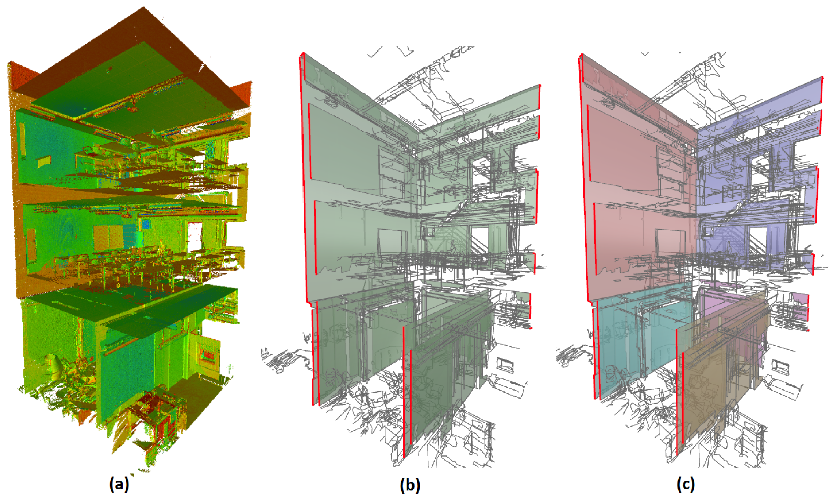
Figure 2.
Workflow of the graph-based wall segments clustering depicting the consecutive steps. The wall segments are shown in green, floor segments in red, and graph edges in bordeaux.
Figure 2.
Workflow of the graph-based wall segments clustering depicting the consecutive steps. The wall segments are shown in green, floor segments in red, and graph edges in bordeaux.

Figure 3.
Illustration of the connected components with the remaining edges in a highly associative configuration. The three clusters are depicted in red, cyan, and purple. The edges are shown in red and the edges between clusters are shown in yellow.
Figure 3.
Illustration of the connected components with the remaining edges in a highly associative configuration. The three clusters are depicted in red, cyan, and purple. The edges are shown in red and the edges between clusters are shown in yellow.
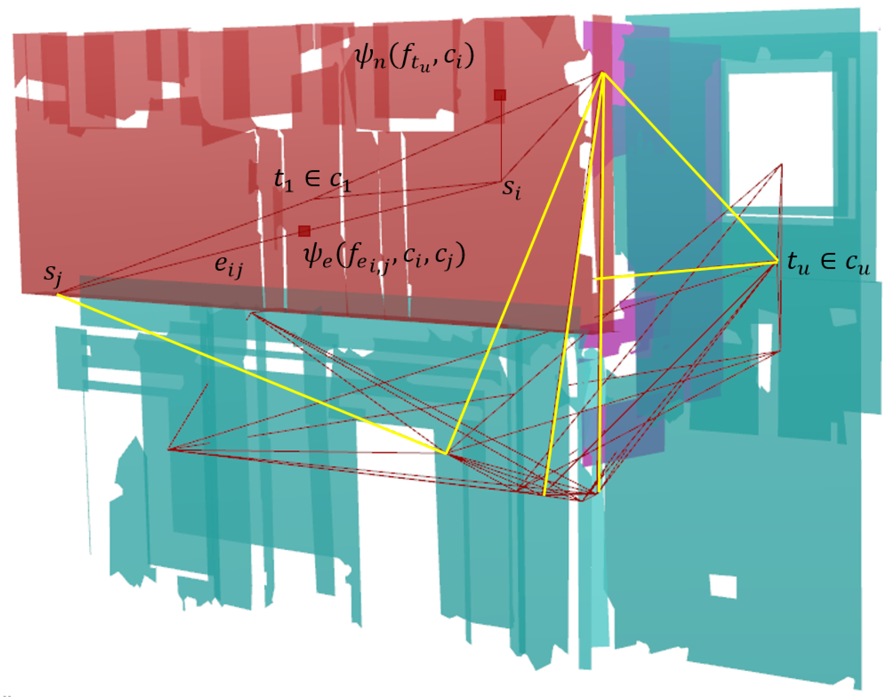
Figure 4.
Illustration of the clustering using conditional random fields within a connected component graph: Given the seeds from the region growing, one of u labels is computed for each s given the factor graph with the edge and node potentials. (a) Representation of the unary and pairwise features and (b) the representation of the factor graph. Decoding results in the assignment of both and to (red cluster).

Figure 5.
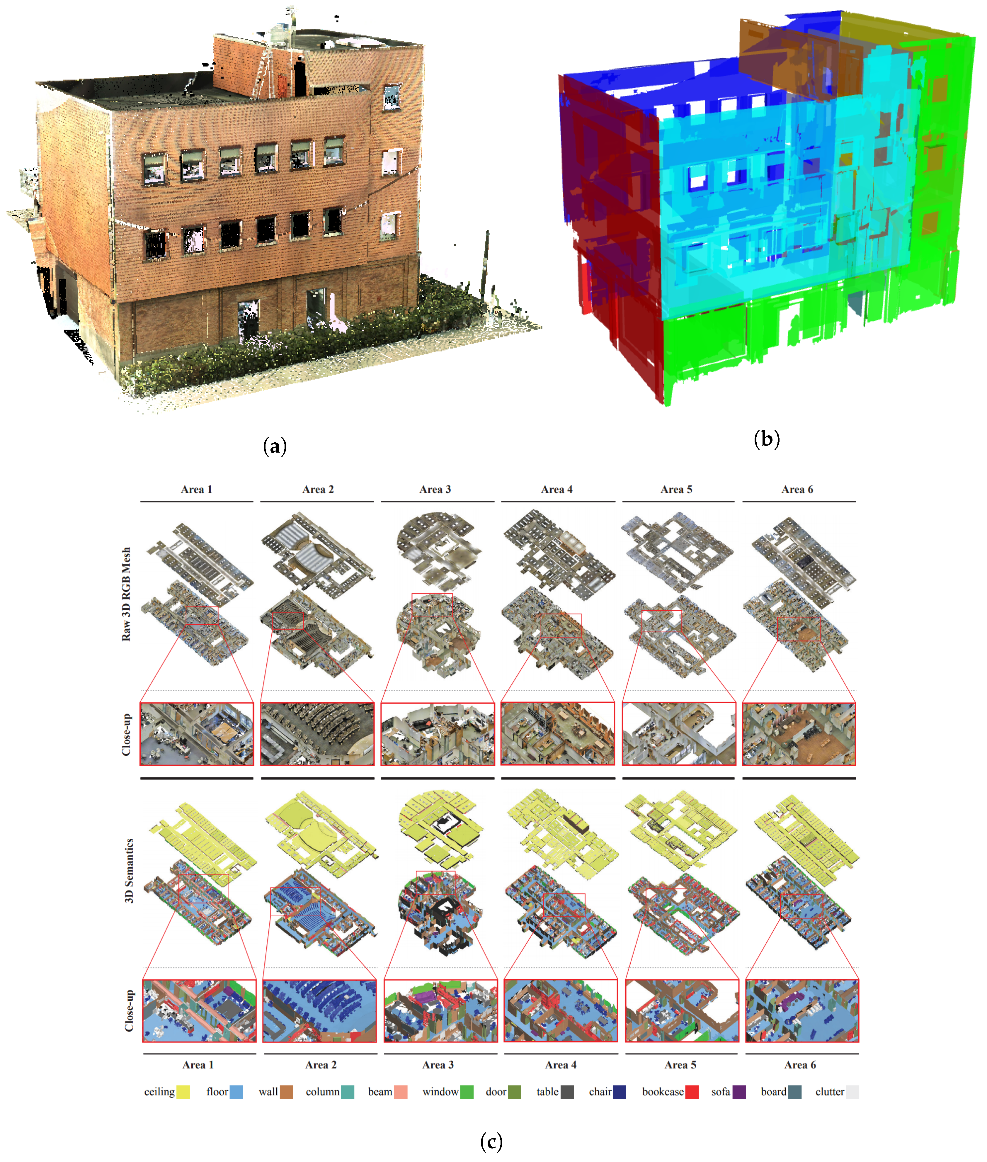
Test data sets for the conditional random fields clustering experiments. (a) Technology campus Ghent point cloud data; (b) Ground truth walls in a separate color; (c) 2D-3D-Semantics (2D-3D-S) benchmark data of Stanford including colored and annotated meshes [40].
Figure 5.
Test data sets for the conditional random fields clustering experiments. (a) Technology campus Ghent point cloud data; (b) Ground truth walls in a separate color; (c) 2D-3D-Semantics (2D-3D-S) benchmark data of Stanford including colored and annotated meshes [40].

Figure 6.
Comparison between the results of the proposed conditional random fields (CRF) clustering algorithm and a conventional region growing algorithm. The seed nodes are represented in yellow and the walls are colored according to their respective clusters.
Figure 6.
Comparison between the results of the proposed conditional random fields (CRF) clustering algorithm and a conventional region growing algorithm. The seed nodes are represented in yellow and the walls are colored according to their respective clusters.

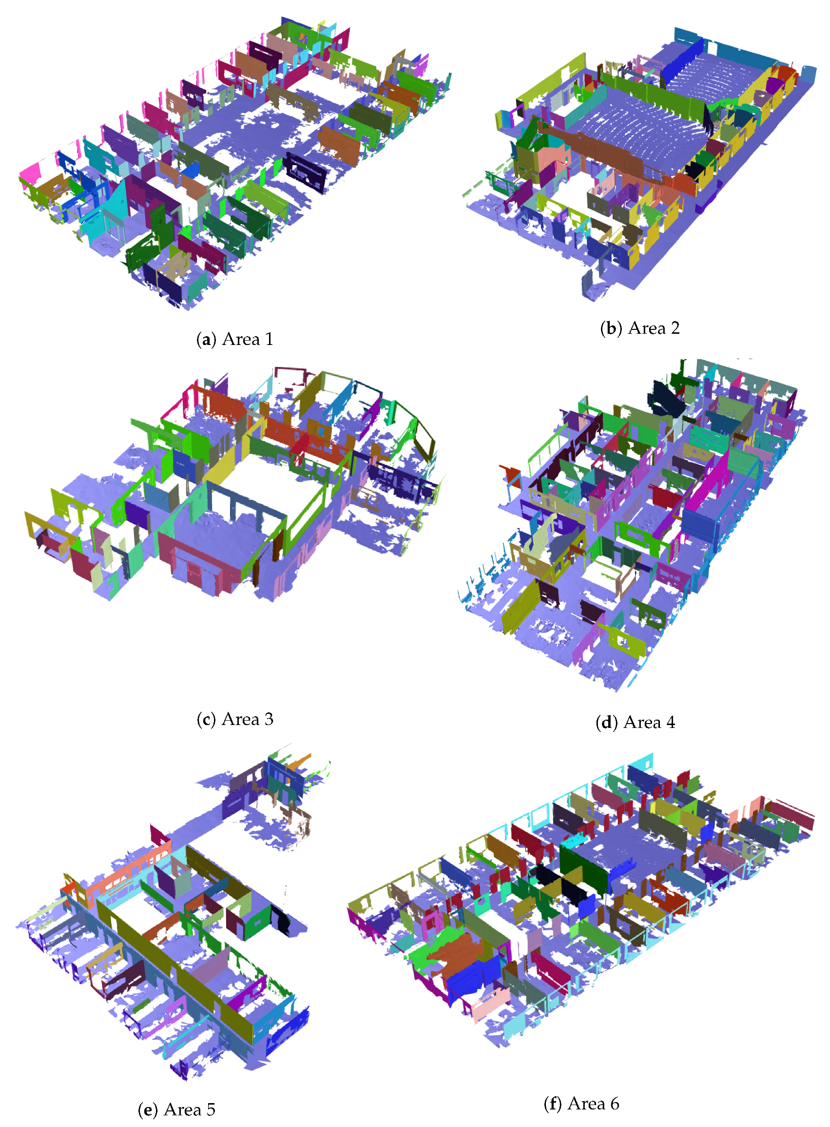
Figure 7.
Overview of the results of the proposed CRF clustering algorithm. Each wall extracted from the connected components is shown in a different color. Valid connected components and singular walls are not shown.
Figure 7.
Overview of the results of the proposed CRF clustering algorithm. Each wall extracted from the connected components is shown in a different color. Valid connected components and singular walls are not shown.

Figure 8.
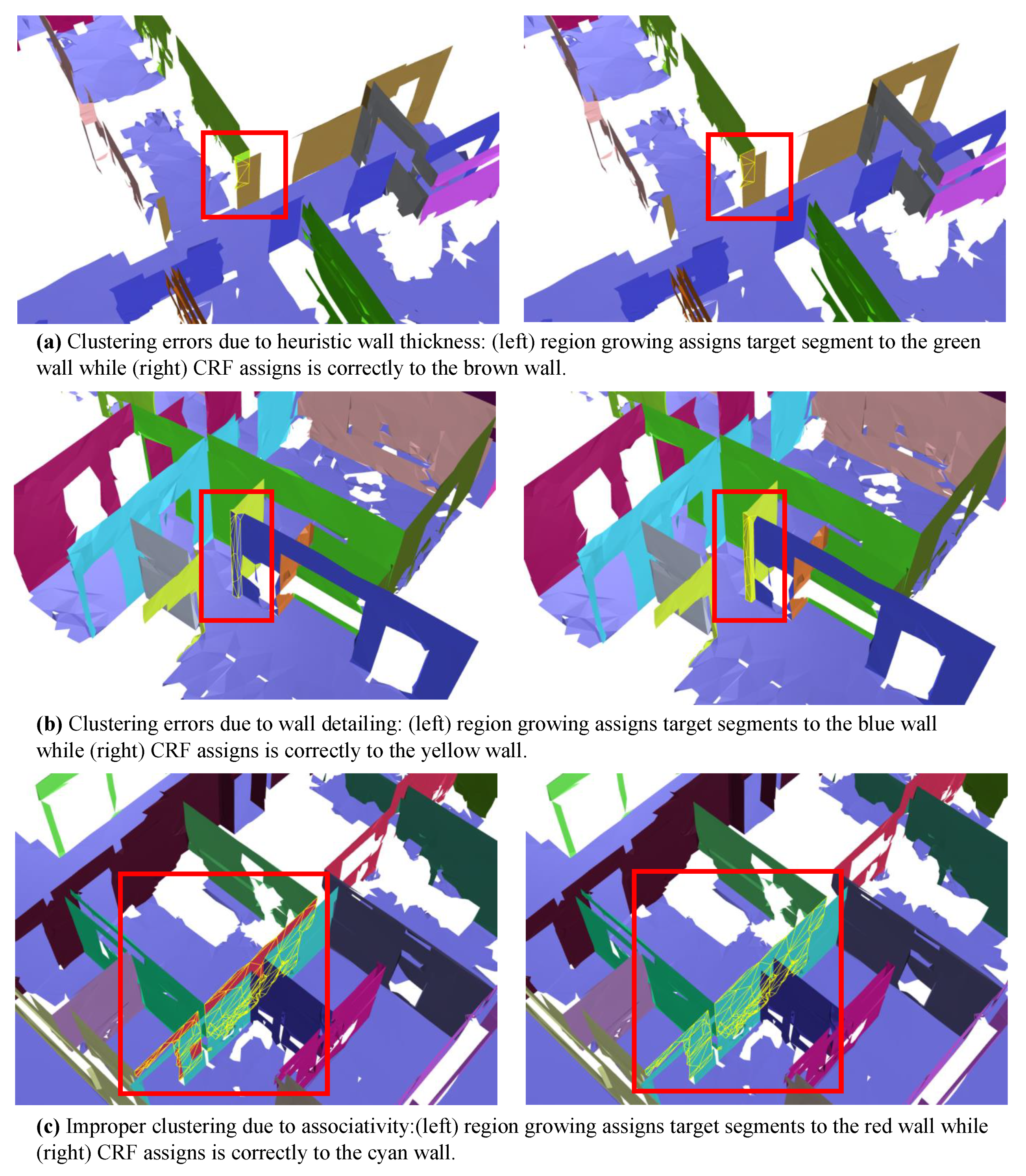
Overview of the difference in clustering between conventional region growing and the proposed CRF method.
Figure 8.
Overview of the difference in clustering between conventional region growing and the proposed CRF method.

Table 1.
Results of the CRF method on the 2D-3D-S dataset.
| Dataset | 3D Points | 3D Meshes | Wall Segments | Wall Objects | Time [s] | Recall [%] | Precision [%] |
|---|---|---|---|---|---|---|---|
| Area 1 | 43,956,907 | 158,500 | 235 | 84 | 4.3 | 94.8 | 86.0 |
| Area 2 | 470,023,210 | 361,830 | 284 | 82 | 12.9 | 80.4 | 89.0 |
| Area 3 | 18,662,173 | 147,420 | 160 | 61 | 2.6 | 96.1 | 76.8 |
| Area 4 | 43,278,148 | 201,735 | 281 | 96 | 6.3 | 89.6 | 90.6 |
| Area 5 | 78,649,818 | 198,220 | 344 | 54 | 2.0 | 89.5 | 89.2 |
| Area 6 | 41,308,364 | 198,590 | 248 | 71 | 4.9 | 93.7 | 85.1 |
| Average | 115,979,770 | 211,500 | 259 | 75 | 5.5 | 90.6 | 86.1 |
Table 2.
Results of the region growing method on the 2D-3D-S dataset.
| Dataset | Connected Components | Potential Seeds | Wall objects | Time [s] | Recall [%] | Precision [%] |
|---|---|---|---|---|---|---|
| Area 1 | 8 | 87 | 84 | 3.6 | 84.8 | 81.0 |
| Area 2 | 6 | 95 | 82 | 10.2 | 76.4 | 83.0 |
| Area 3 | 4 | 65 | 61 | 1.9 | 88.1 | 76.3 |
| Area 4 | 6 | 96 | 96 | 4.3 | 88.6 | 89.5 |
| Area 5 | 6 | 57 | 54 | 2.0 | 86.7 | 86.1 |
| Area 6 | 4 | 73 | 71 | 4.1 | 85.6 | 83.7 |
| Average | 6 | 79 | 75 | 4.4 | 85.0 | 83.3 |
© 2019 by the authors. Licensee MDPI, Basel, Switzerland. This article is an open access article distributed under the terms and conditions of the Creative Commons Attribution (CC BY) license (http://creativecommons.org/licenses/by/4.0/).
Share and Cite
MDPI and ACS Style
Bassier, M.; Vergauwen, M. Clustering of Wall Geometry from Unstructured Point Clouds Using Conditional Random Fields. Remote Sens. 2019, 11, 1586. https://0-doi-org.brum.beds.ac.uk/10.3390/rs11131586
AMA Style
Bassier M, Vergauwen M. Clustering of Wall Geometry from Unstructured Point Clouds Using Conditional Random Fields. Remote Sensing. 2019; 11(13):1586. https://0-doi-org.brum.beds.ac.uk/10.3390/rs11131586
Chicago/Turabian StyleBassier, Maarten, and Maarten Vergauwen. 2019. "Clustering of Wall Geometry from Unstructured Point Clouds Using Conditional Random Fields" Remote Sensing 11, no. 13: 1586. https://0-doi-org.brum.beds.ac.uk/10.3390/rs11131586
Note that from the first issue of 2016, this journal uses article numbers instead of page numbers. See further details here.