Flood Spatial Modeling in Northern Iran Using Remote Sensing and GIS: A Comparison between Evidential Belief Functions and Its Ensemble with a Multivariate Logistic Regression Model

Abstract

Floods are some of the most dangerous and most frequent natural disasters occurring in the northern region of Iran. Flooding in this area frequently leads to major urban, financial, anthropogenic, and environmental impacts. Therefore, the development of flood susceptibility maps used to identify flood zones in the catchment is necessary for improved flood management and decision making. The main objective of this study was to evaluate the performance of an Evidential Belief Function (EBF) model, both as an individual model and in combination with Logistic Regression (LR) methods, in preparing flood susceptibility maps for the Haraz Catchment in the Mazandaran Province, Iran. The spatial database created consisted of a flood inventory, altitude, slope angle, plan curvature, Topographic Wetness Index (TWI), Stream Power Index (SPI), distance from river, rainfall, geology, land use, and Normalized Difference Vegetation Index (NDVI) for the region. After obtaining the required information from various sources, 151 of 211 recorded flooding points were used for model training and preparation of the flood susceptibility maps. For validation, the results of the models were compared to the 60 remaining flooding points. The Receiver Operating Characteristic (ROC) curve was drawn, and the Area Under the Curve (AUC) was calculated to obtain the accuracy of the flood susceptibility maps prepared through success rates (using training data) and prediction rates (using validation data). The AUC results indicated that the EBF, EBF from LR, EBF-LR (enter), and EBF-LR (stepwise) success rates were 94.61%, 67.94%, 86.45%, and 56.31%, respectively, and the prediction rates were 94.55%, 66.41%, 83.19%, and 52.98%, respectively. The results showed that the EBF model had the highest accuracy in predicting flood susceptibility within the catchment, in which 15% of the total areas were located in high and very high susceptibility classes, and 62% were located in low and very low susceptibility classes. These results can be used for the planning and management of areas vulnerable to floods in order to prevent flood-induced damage; the results may also be useful for natural disaster assessment.

1. Introduction

A natural disaster is a major adverse event resulting from the natural processes of the Earth. These can include floods, hurricanes, tornadoes, volcanic eruptions, earthquakes, tsunamis, etc. A natural disaster can cause loss of life and damage to property, which typically results in economic damage, the severity of which depends on the affected population’s resilience, or ability to recover, and also on the available infrastructure. Among natural disasters, floods are considered to be one of the most devastating [1], and an accurate assessment of its risks is hampered by a lack of data and knowledge about flood losses at different scales [2]. During a heavy rainfall event, the amount of flow discharge in a river increases rapidly and the water level will rise above its normal bed, covering the flood plain and surrounding areas [3]. 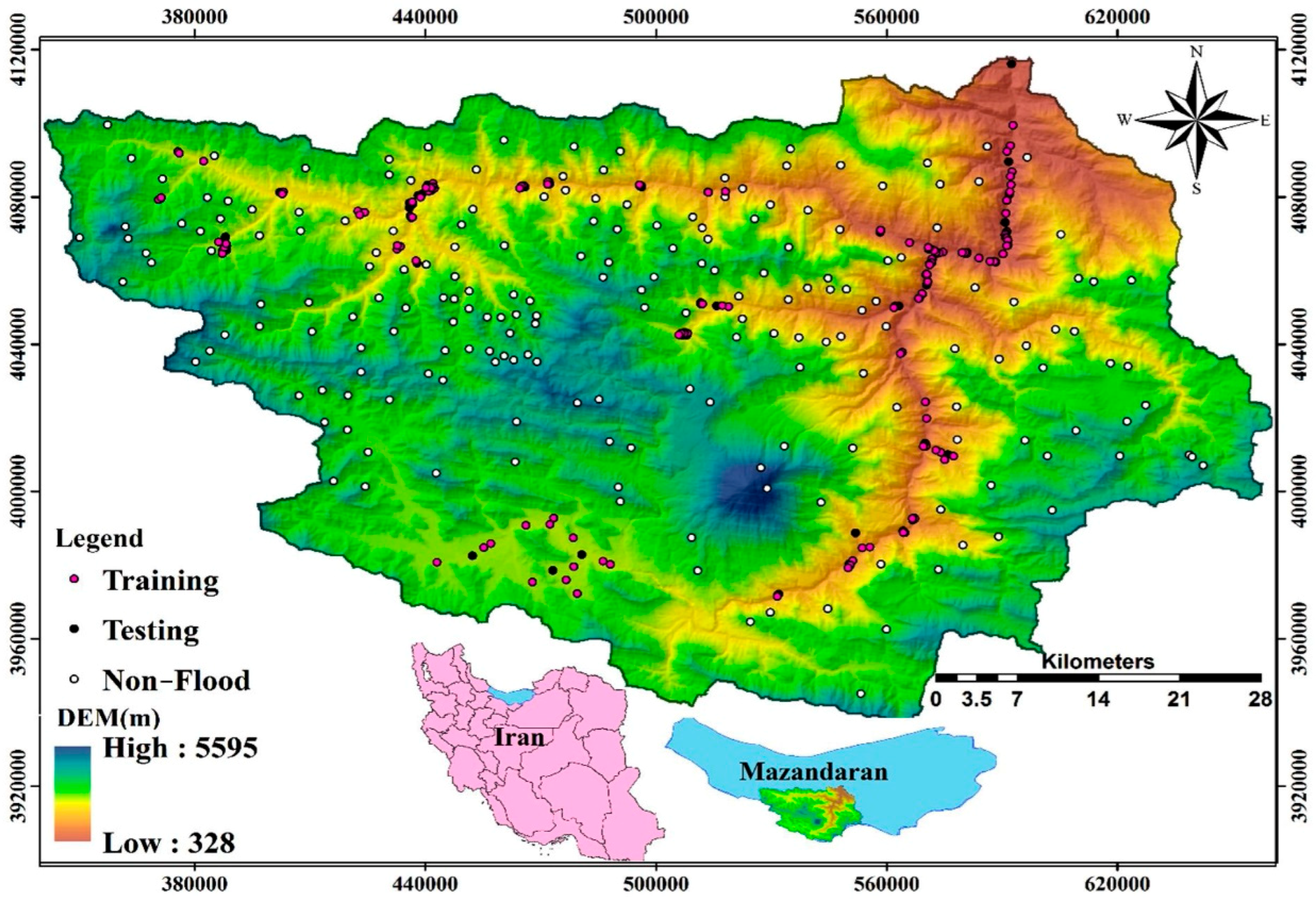Life-threatening water overflow in residential areas is a common occurrence in Iran after earthquakes (http://www3.irna.ir/fa/NewsPrint.aspx?ID=214943), and catastrophic flooding events happen annually in the Mazandaran, Guilan, and Golestan Provinces in Northern Iran. Due to the high flood-frequency in this region, to prevent loss of life and property damage, areas with a high risk of flooding must be recognized according to flood susceptibility maps [4]. The primary difference between flood susceptibility and flood inundation maps is that flood susceptibility maps (FSM) only show the areas that have a high potential for flooding, while flood inundation maps can identify flood-prone areas based on different flood depths [5,6].

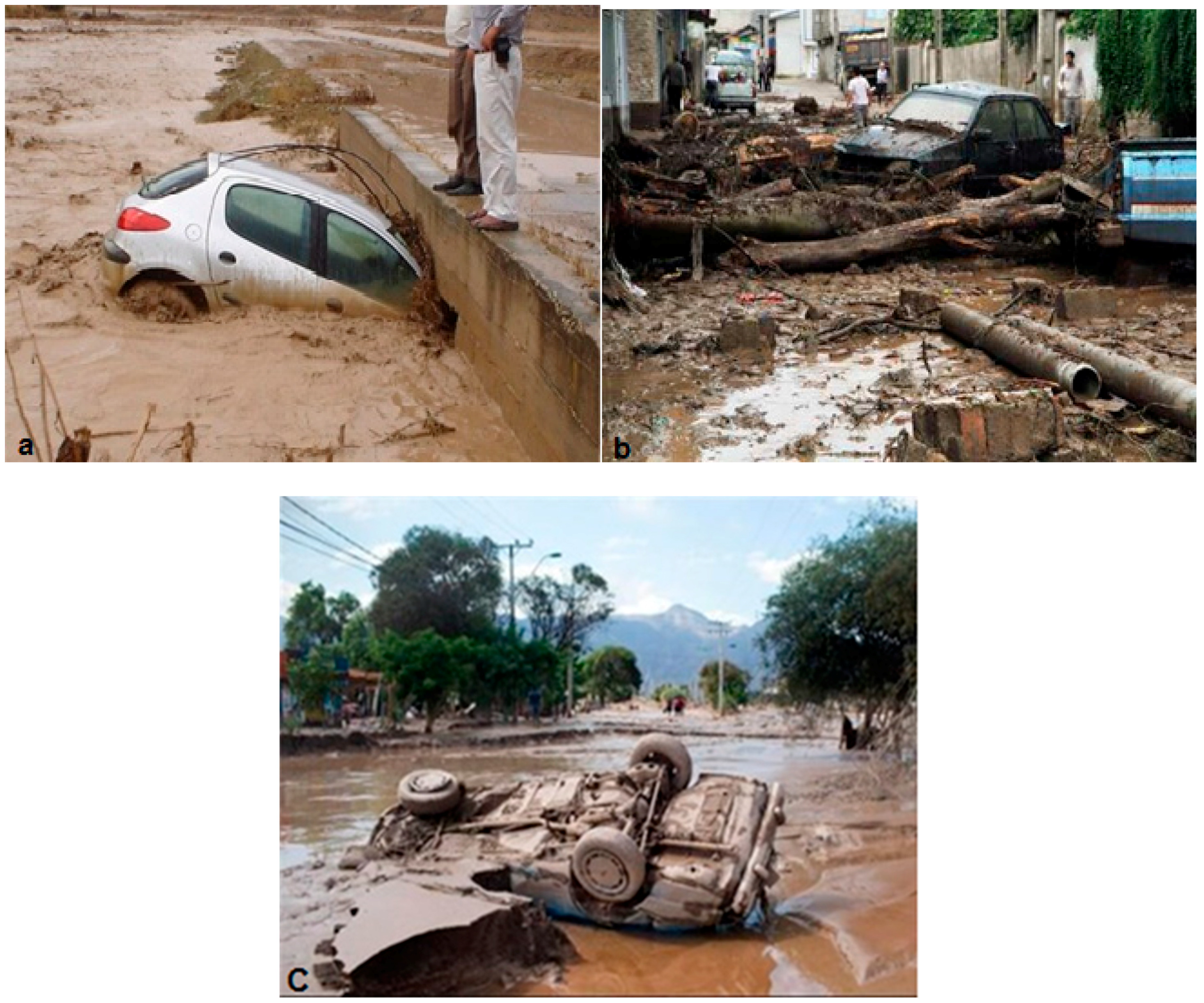
On a global scale, floods are the most destructive natural disasters, causing the highest number of deaths and damage; in fact, Opolot [7] noted that almost 99 million people around the world were affected by floods between 2000 and 2008. In the most recent decade, the occurrence of repeated flood events in the northern part of Iran reached its historical maximum, with the rate and extent of damage increasing every year. Examples of recent floods in the Mazandaran Province and its cities include Noshahr City in 1995, 2003, and 2012, Neka City in 1999, Behshar City in 2013, and Sari City also in 2013. The flood in Neka City caused more than $1,000,000 worth of damage to agricultural lands including wheat, barley, and rice fields. The arable lands of about 28 villages, with an area of 80 ha, were also destroyed in the Chahardangeh District, Sari, while 150 ha of agricultural lands were destroyed in Klijan Restagh in Sari City. Hence, identification and evaluation of sensitive areas are essential in order to prevent and mitigate flood damages and losses [4]. Hydrologists have used several models to prepare flooding maps, but many of these models are data intensive or difficult to calibrate; however, some of the models are still required to understand the physical processes occurring within the catchment [8].

In recent years, many statistical and probabilistic models have been tested to prepare flood susceptibility maps [9,10]. Geographic Information System (GIS) has been used as an effective tool for spatial analysis and data manipulation due to its ability to handle large amounts of spatial data [11]. Specifically, the combination of statistical and probabilistic models with Remote Sensing (RS) and GIS has been widely used by different researchers [1,12]. Additionally, some scientists and researchers have studied natural disasters, specifically floods and FSM, with the help of RS and GIS, using different models such as Decision-Tree (DT) [6,13], Support Vector Machine (SVM) [14,15], Frequency Ratio (FR) [16,17], Evidential Belief Function (EBF) [18,19,20], EBF-AHP (Analytical Hierarchy Process) [21], Logistic Regression (LR) [22], Shannon’s entropy and weights-of-evidence [23], Artificial Neural Networks (ANN) [23], AHP [23,24], Random Forest [3,23], and Adaptive Neuro-Fuzzy Inference System (ANFIS) [25,26]. Recently, Khosravi et al. [27] compared the prediction power of the data mining algorithms of Naïve Bayes and Naïve Bayes Tree with three Multi-Criteria Decision-Making (MCDM) analysis techniques (VIKOR, TOPSIS, and SAW). Their finding show that although MCDM models could predict flood-prone areas, the data mining algorithms had a higher prediction power than MCDMs since MCDMs rely on expert opinion. Arabameri et al. [28] applied an EBF model to the generation of flood susceptibility maps and compared the results with FR, TOPSIS, and VIKOR models, concluding that the EBF model performed best.

Recently, hybrid machine learning methods have been applied to studies relating to the spatial prediction of natural hazards such as landslides [12,20,29,30,31,32,33,34,35,36,37,38,39,40,41,42,43,44,45,46,47,48,49], wildfires [50], sinkholes [51], droughts [52], gully erosion [53,54], and groundwater [55,56] and land/ground subsidence [12]. An advantage of the ensemble algorithms is that they have a higher goodness-of-fit and prediction accuracy than individual or single-based methods/algorithms.

Khosravi et al. [57] stated that (1) every model has its advantages and disadvantages, (2) model performance depends on the data, accuracy and model structure, and (3) there is no universal guideline specifying which model should be applied in any given scenario; therefore, several models should be applied and the best of them used for further analysis. According to the literature, many machine learning and data mining algorithms have recently been applied in the field of natural hazards assessment, however, there is no consensus among researchers with regard to which model is best. Some research shows that bivariate statistical models demonstrated better predictive power than both machine learning and data mining algorithms [23]; this is because machine learning and data mining algorithms are more complex and require an expert to perform accurate simulations. Therefore, bivariate models, which are very simple to run with similar or sometimes superior predictive power, can be used as adequate substitutes.

At present, the EBF method is rarely applied for flood analysis, though it has been used for other categories of natural disasters such as landslide susceptibility assessment [21,33,58], and land subsidence [12,59], as well as having been used to predict groundwater potential zones [19,60].

The main purpose of this research is to evaluate the possibilities of using the EBF method to generate flood susceptibility maps and to assess the strengths and weaknesses of this method, as EBF has rarely been used for floods but has shown high accuracy in previous studies involving natural hazards mapping. The specific objectives of the current study include, (i) determining the most significant factors in each model, (ii) application of a bivariate statistical model, EBF, to produce new ensemble models, in combination with a statistical model, LR, in order to generate a more accurate flood susceptibility map, (iii) detection of the flood-prone areas within the study region for improved management during flood occurrence. In general, river flooding is a common natural disaster in the southern Caspian Sea, especially in the Haraz catchment; the results of the current study will be useful for land-use planning and management for future flood mitigation in the Haraz Watershed.

2. Study Area

The Haraz Catchment is located between the longitudes of 51°43′ to 52°36′E and the latitudes of 35°45′ to 36°22′N. The study area lies south of Amol City, Mazandaran Province, Iran (Figure 1) and has an area of 4014 km². The minimum and maximum elevations are 300 and 5600 m, respectively. Average annual rainfall in the region was 723.07 mm in 2006 and 831.38 mm in 2012. The important residential centers of the Haraz Catchment are Polur, Tashal, Tiran, Rineh, Kandovan, Abasak, Gaznak, Baladeh, and Noor. The main causes of flooding in these areas include high-intensity rainfall over a short time-period, land-use changes in rangelands (e.g., deforestation or conversion of agricultural land and garden to residential areas), and the lack of effective management to prevent flooding. The maximum rainfall occurs in January, February, March, and October; with October being the wettest month with an average rainfall of 160 mm [61].

3. Methodology

3.1. Data Used

3.1.1. Flood Inventory Map

To estimate the incidence of future floods in the study area, it is essential to analyze the occurrence of previous floods [62]. The accuracy of historical flood data has a strong influence on the legitimacy of predictive flood-potential mapping [63]. In this study, the flood inventory map was prepared based on data from flood events occurring in the years 2004, 2008, and 2012 (Mazandaran Regional Water Organization); this data was obtained through analysis of historical documentation, aerial photographs, and field surveys. In total, 211 flooding locations and 211 non-flooding locations were selected. A ‘non-flooding location’ refers to an area with relatively high elevation (e.g., hills and mountains) that is not affected by flooding, and these points were identified using a topographic map and Google Earth [64]. The resultant flood inventory map was then divided into two parts for training (151 flood locations, 70% of sampled land area) and validation (60 flood locations, 30% of sampled land area) randomly [65]. Selected photos of floods in the northern part of the country are shown in Figure 2a–c.

3.1.2. Multicollinearity Diagnosis

After determining the flood-conditioning factors, it is important to consider potential problems associated with multicollinearity between independent variables [65]. If multicollinearity in the regression equation is high, it means that there is a high correlation between independent variables (inter-dependent) and, despite a high R², the model will not have a high validation accuracy. The exponent of the linear relationship between independent variables of the model is measured by an index that is called the tolerance, which is between 0 and 1. The Variance Inflation Factor (VIF) and tolerance are the most important indicators to consider when attempting to detect multicollinearity [66]. A tolerance of less than 0.2 or a VIF greater than 5 indicates a multicollinearity problem [66].

3.1.3. Flood-Conditioning Factors

In susceptibility mapping for floods or other natural disasters, it is necessary to define a series of conditioning factors [5,67]. In this study, ten conditioning factors were applied. Altitude, slope angle, plan curvature, the topographic wetness index (TWI) and stream power index (SPI) were derived from the ASTER Global DEM (ASTER GDEM) (https://gdex.cr.usgs.gov/gdex/), while distance from river, rainfall, geology, land-use, and Normalized Difference Vegetation Index (NDVI) were prepared from Operational Land Imager (OLI) of Landsat 8 image (

Table 1. Factors used in spatial modeling for flood susceptibility assessment in the study area.

Classification	Sub-Classification	Source of Data	GIS Data Type	Derived Map	Scale or Resolution
Flood inventory map	Flood inventory	Mazandaran Regional Water Authority Field surveys	Polygon coverage	Seed cells	28 m × 28 m
ASTER GDEM *	Slope angle	DEM *	GRID *	Slope angle	28 m × 28 m
	Altitude	DEM	GRID	Elevation	28 m × 28 m
	Plan curvature	DEM	GRID	Curvature	28 m × 28 m
	SPI *	DEM	GRID	Sediment transport index	28 m × 28 m
	TWI *	DEM	GRID	Topographic wetness index	28 m × 28 m
	Distance from river	DEM	Line coverage	Distance to river	28 m × 28 m
Geology Map	Geology	Geological map	GRID	Lithology	1:100,000
Land use type	Land use	OLI * of Landsat 8 image	GRID	Land use	30 m × 30 m
	NDVI *	OLI of Landsat 8 image	GRID	NDVI	30 m × 30 m
Precipitation	Rainfall	20 years (1991–2011) from 17 rain gauges (IDW) *	GRID	Rainfall	28 m × 28 m

* GRID (graphic design); ASTER GDEM (ASTER Global DEM); DEM (Digital Elevation Model); NDVI (Normalized Difference Vegetation Index); TWI (Topographic Wetness Index); SPI (Stream Power Index); OLI (Operational Land Imager); IDW (Inverse Distance Weighting).

) and then converted into 28 × 28 m cell sizes based on a Digital Elevation Model (DEM).

Topographic Factors

A DEM with a spatial resolution of 28 × 28 m was used to provide primary and secondary features such as altitude (Figure 3a), slope angle (Figure 3b), and plan curvature (Figure 3c) in ArcGIS 10.1. Altitude, slope angle, and plan curvature factors were classified into nine, five, and three classes, respectively [18], based on a natural break classification scheme [68]. Flat areas with low slope and low altitude classes have a higher potential for flooding.

Water-Related Factors

Factors such as the topographic wetness index (TWI) and stream power index (SPI) were prepared using a DEM in the SAGA-GIS 2.8 software. TWI is the accumulation of flow at any location in the catchment, with consideration of downstream flow trends due to gravity [69]. Equation (1) was proposed by Moore et al. [70] to calculate the TWI:

$$TWI=\ln (A_S/\tan \beta )$$

(1)

where A_S is the specific area of the catchment in m²/m of the catchment and β is the slope angle in degrees. The TWI map is shown in Figure 3d. Figure 3e shows the SPI, which is the measurement of the erosive power of water flow, which is shown in Equation (2) [70]:

$$SPI=(A_S\times \tan \beta )$$

(2)

To create the layer for the distance from the river factor, the digital map of the river was edited using the multi-ring buffer command in ArcGIS 10.1. Subsequently, this layer was divided into six classes: 500, 1000, 1500, 2000, 2500, and >2500 m (Figure 3f). Distance from the river (or distance of the measurement points from the river) has a major role in the distribution and magnitude of floods in the area [71]. In the northern part of Iran, as a result of insufficient infiltration and percolation due to changes in soil characteristics, vegetation coverage, and ground surface slope, high-intensity rainfall events generate large amounts of runoff in the vicinity of the nearby river, causing catastrophic flood events in downstream areas with lower topographic gradients [72].

Twenty years of rainfall data (1991–2011) from 17 stations inside and outside of the study area were used to generate an annual rainfall map. Several interpolation methods, such as kriging (simple and ordinary), inverse distance weighting (IDW) with a power of 1 to 5, radial function with kernel functions of completely regularized spline and spline with tension, were compared to find the best method for mapping the rainfall data. The simple kriging method was selected as the best method because it produced the lowest Root Mean Square Error (RMSE) and Mean Absolute Error (MAE) [16]. The rainfall map of the study area was ultimately divided into nine classes [73] (Figure 3g).

Physical Factors

In general, geology plays a significant role in flood susceptibility due to the variable sensitivity of lithological units. Areas with hard and resistant rocks, as well as highly-permeable soils, have low channel densities [74,75]. The geology layer of the study area, in GIS shapefile format, was obtained from the Mazandaran Regional Water Organization and was originally prepared by the Geological Survey Department in Iran.

The ability of rock formations to resist chemical and mechanical weathering were classified according to the degree of permeability, into low, moderate, and high classes [76]. Finally, the geological map of the study area was classified into three groups [16,77] and is presented in Figure 3h and

Table 2. The lithology of the Haraz Catchment.

Lithology	Formation	Code	Permeability
Rockfall	-	Qf	Low
Basic flow, pyroclastics	-	Pv	Low
Rocks, marl, conglomerate, Paleocene	Dorud	Pd	Low
Rocks, marl, conglomerate, Paleocene	Fajan	Pecf	Low
Thick dolomite to form massive, limestone	Elika	TRe2	Low
Mafic volcanic rocks	-	TRv3	Low
Gabbro	-	Tgb	Low
Basalt	-	Kv	Low
Basalt, diabase, pyroclastic rocks and pyroclastic volcanic rocks	-	Kv1	Low
Tuff, basaltic andesite pyroclastic	-	Kv2	Low
Cut from multiple sources, Paland formation	Paland	TRb	Low
Basalt and olivine	-	Qv1	Low
Agglomerate and andesite tuff	-	Qv2	Low
Damavand magma, Andesite trachyte	-	Qv3	Low
Quartz-Diorite	-	Qd	Low
Rhyolite	-	Rh	Low
Trachyte	Eilka	TR	Low
Dacite	-	da	Low
Middle tuff member: pyroclastics	Karaj	Ekt2	Low
Trachyandesite, trachybasalt, basanite	Karaj	Evkt2	Low
Pyroclastic and andesite	Karaj	EA	Low
Dacite, pyroclastic	-	Ezt2	Low
Tuff, volcanic rock	Karaj	Ek	Low
Scree, talus fans	-	Qs	Moderate
Scree	-	Qsc	Moderate
Marine conglomeratic terraces	-	Qt	Moderate
A thin layer of cream limestone, shale, limestone, Elika formation	Elika	TRe1	Moderate
Sandstone, shale, limestone, quartzite, make peace	Fajan	Pefvmc	Moderate
Limestone, marly and sandy shales	Nesen	Pn	Moderate
Fusulina limestone, dolomitic limestone	Ruteh	Pr	Moderate
Santonian limestone	-	K2l	Moderate
Limestone, marl, limestone, silty marl	-	K2plm	Moderate
Cast locally with the layers of dolomitic limestone and shale	-	Kgl	Moderate
Limestone and marl	-	Kl-m	Moderate
Orbitolina Limestone	Tiz Kuh	Klt	Moderate
Nummulitic limestone	Ziarat	Ez	Moderate
Conglomerate	Fajan	Ef	Moderate
Old terraces	-	Qt1	High
Undifferentiated Quaternary deposits	-	Q	High
Loose alluvium in the river channels	-	Qal	High
Landslide	-	Qlan	High
Moraines (glacial deposits)	-	Qm	High
Calcareous and siliceous shales	Karaj	Eksl	High
Younger gravel fans and terraces	-	Qt2	High
Loess	-	Qt2c	High
Sinter deposits	-	Qtr	High
Marl	Mila	E-m	High
Gypsum	Kand	Eg	High

.

The land-use and NDVI maps were prepared using satellite images from Landsat 8 OLI (taken from the National Geography Organization of Iran) from 2013. The land-use map was classified into seven categories, consisting of rangeland, bare land, forest, garden, irrigated land, residential areas, and water-bodies; this was done using a Neural Network Algorithm (ANN) and through supervised classification in Environment for Visualizing Images (ENVI 5.1) software (Figure 3i).

The NDVI map shows the surface coverage of live vegetation. The vegetation index exists as a proportional output between −1 and +1. The NDVI values (Figure 3j) were calculated using Equation (3) [78]:

$$NDVI=(NIR-VIS)/(NIR+VIS)$$

(3)

where VIS and NIR are the spectral reflectance measurements acquired in the red and near-infrared bands of the electromagnetic spectrum, respectively.

All of the aforementioned flood conditioning factors were converted to a grid comprised of 28 × 28 m cells.

3.2. Application of Models

Flood susceptibility analyses are highly important studies in the field of river hydrology [64,79]. In this study, the flood susceptibility analysis was carried out using EBF, EBF from LR, EBF-LR (Enter) and EBF-LR (Stepwise) methods. Four steps were taken to prepare the flood susceptibility maps of the study area: (1) Data was collected, and a spatial database of conditioning factors associated with flood occurrences was created, (2) the relationship between conditioning factors and flood locations was determined, (3) flood susceptibility maps were prepared using the different algorithms, and (4) the results were validated using success and prediction-rate curves and visual interpretation. The methodology of this research is presented as a flowchart in Figure 4.

3.2.1. Evidential Belief Function (EBF) Model

The EBF model is based on the Dempster–Shafer Theory of Evidence [80,81]. Therefore, to implement the EBF model, the layers of the conditioning factors were transformed into evidential data layers and then integrated using knowledge of the spatial relationships between the flood occurrences and factors influencing the flooding in order to generate a predictive Flood Susceptibility Index (FSI) map. One of the advantages of this model is that both the predicted flood and flooding zone outputs exist within the same degree of uncertainty [82]. The EBF model is composed of four functions, namely: Bel (degree of Belief), Dis (degree of Disbelief), Unc (degree of Uncertainty) and Pls (degree of Plausibility) [18,83]. Four maps of Bel, Dis, Pls, and Unc were used for the assessment of the ten factors influencing flooding. Each map shows the probability of flood occurrences. The integration of all the factors shows the level of prediction accuracy. The EBF model was run using the following steps [84]. Equations (5) and (6) show how to achieve the results of Bel:

$$\lambda (Tp)=N/D=[N(LIEij)/N(L)]/[N(Eij)-N(LIEij)/(N(A)-N(L)]$$

(4)

$$Bel=\lambda (Tp)Eij/\sum \lambda (Tp)Eij)$$

(5)

where, N(L∩Eij) is the number of flood pixels in each class, N(L) is the total number of floods, N(Eij) is the number of pixels of each class, N(A) is the total pixels, and N and D are the proportions of flood event areas and non-flood areas, respectively.

Similarly, Dis values were also obtained through Equations (7) and (8), as shown below:

$$\lambda (T\overline{p})Eij=K/H=[(N(L)-N(L\cap Eij))/N(L)]/[N(A)-N(L)-N(Eij)/(N(A)-N(L)]$$

(6)

$$Dis=\lambda (T\overline{p})Eij/({\displaystyle \sum \lambda (T\overline{p})Eij)}$$

(7)

where K is the proportion of flooding that does not occur, and H is the proportion of non-flooding occurrence areas in other attributes outside the class.

Equations (4) and (6) were applied for all classes of factors influencing floods, and Equations (5) and (7) were used for Bel and Dis results. According to Dempster [80], the main part of the Theory of Evidence is provided by Bel being equal to the lower probability and Pls being equal to the upper probability; therefore, Pls is greater than or equal to Bel. According to Althuwaynee et al. [18], the three primary functions associated with the theory of Dempster–Shafer are as follows (1) Basic probability assignment function (BPA), (2) Belief function (Bel), and (3) Plausibility function (Pls). Generally, the other parameters were calculated, as shown in Equations (8), (9), and (10):

Pls − Bel = Unc

(8)

Dis = (1 − Pls) or (1 − Unc)

(9)

Bel + Unc + Dis = 1

(10)

3.2.2. Logistic Regression (LR) Model

Logistic regression is one of the Multivariate Statistical Analysis (MSA) models, which considers several parameters (e.g., slope, altitude, and plan curvature) that may affect the likelihood of flooding [85,86]. The purpose of using an LR model in this study was to determine the appropriate model for defining the relationships between the dependent variable and the factors affecting floods, in order to generate coefficients for each variable [87]. Therefore, in this study, 70% of the flood training points and ten flood-conditioning factors were entered into the model as the dependent and independent variables, respectively [88]. Statistical Package for Social Science software (SPSS18) was used to run the LR model using the Forward Conditional (stepwise) and Enter methods. In the Forward method, variables were entered into the model individually, and the results were evaluated based on the correlation between flood occurrence and individual variables; if there were no significant correlation, then the variable would be eliminated from the model [89]. The Forward Conditional calculations were based on significant probability (Sig) in the LR model, with Sig <0.05 indicating that the flood conditioning factor or independent variable had a statistically significant impact on flooding [73]. In the Enter method, all factors were entered into the model regardless of their correlation with flood occurrence. One of the advantages of LR models is that the data do not require a normal distribution, and the conditioning factors can be either continuous or discrete. Quantitatively, the relationship between flood occurrence and its dependency on several independent variables can be computed using Equation (11) as follows [19]:

$$P(event)=\frac{e^Z}{(1+e^Z)}$$

(11)

where P is the probability of an occurrence. As the value of Z changes from −∞ to +∞, the probability of occurrence fluctuates between 0 and 1. Z is the linear combination function of affecting factors (Equation (12)) that indicate the linear relationship, and b0 is the cutoff value of the model.

$$Z=b_0+b_1{x}_1+b_2{x}_2+\dots +b_n{x}_n$$

(12)

The general equation of an LR model is given by Equation (13):

$$Y=Logit(p)=\ln \left(\frac{p}{1-p}\right)=b_0+b_1{x}_1+b_2{x}_2+\dots +b_n{x}_n$$

(13)

where Y is the probability of flooding, b_n (i = 0, 1, …, n) are the estimated coefficients from the sample data, n is the number of independent variables, and X_n (i = 0, 1, …, n) are the independent variables. Using an LR model individually may be insufficient since this model lacks the capacity to weight each factor [73]; therefore, the EBF and LR models were combined to assess the probability of flooding events in the study area.

3.3. Validation of the Models

Validation of the developed maps is an essential step in the identification of flood-prone areas, as well as in the determination of map quality [90]. Without validated maps, the models and their results would have no scientific significance [19,91]. In this study, the receiver operating characteristics (ROC) curve was used for model validation. The area under the ROC curve (AUC) was used for the evaluation and quantitative comparison of the methods used for flood susceptibility mapping. In this study, 70% of the chosen flood locations were used for model training, and the remaining 30% were used for model validation. The results of the developed flood susceptibility maps (FSMs) were compared with existent flood positions using success-rate and prediction-rate curves [91], and their accuracy was evaluated.

4. Results

4.1. Flood Susceptibility Mapping Using the EBF Model

The EBF model was used to determine the level of correlation between the flood occurrences and flood factors (

Table 3. Spatial relationships among conditioning factors and flooding occurrence extracted by the EBF method.

Factor	Class	No. of Pixels in Domain	Percentage of Domain	No. of Floods	Percentage of Floods	Bel	Dis	Unc	Pls
Altitude (m)	328–350	112	0.02	0	0.00	0.000	0.108	0.892	0.892
	350–400	242	0.04	0	0.00	0.000	0.108	0.892	0.892
	400–450	466	0.08	2	1.32	0.255	0.107	0.638	0.893
	450–500	651	0.11	5	3.31	0.458	0.104	0.438	0.896
	500–1000	11,230	1.98	46	30.46	0.243	0.077	0.680	0.923
	1000–2000	78,535	13.82	43	28.48	0.032	0.090	0.878	0.910
	2000–3000	282,516	49.70	55	36.42	0.012	0.136	0.852	0.864
	3000–4000	188,954	33.24	0	0.00	0.000	0.162	0.838	0.838
	>4000	5722	1.01	0	0.00	0.000	0.109	0.891	0.891
Slope angle (in Degrees)	0–5	21,626	3.80	45	29.80	0.577	0.138	0.285	0.862
	5–10	43,417	7.63	45	29.80	0.287	0.144	0.569	0.856
	10–15	73,134	12.86	23	15.23	0.087	0.184	0.729	0.816
	15–25	203,899	35.87	25	16.55	0.034	0.246	0.720	0.754
	>25	226,352	39.82	13	8.60	0.016	0.288	0.696	0.712
Plan Curvature (100/m)	Convex	231,228	40.67	23	15.23	0.116	0.469	0.414	0.531
	Flat	118,098	20.77	44	29.13	0.436	0.294	0.271	0.706
	Concave	219,102	38.54	84	55.62	0.448	0.237	0.315	0.763
TWI	1.8–2	72,186	12.70	3	1.99	0.007	0.123	0.869	0.877
	2–3	143,920	25.32	4	2.65	0.005	0.143	0.852	0.857
	3–4	135,369	23.81	9	5.96	0.012	0.136	0.853	0.864
	4–5	95,640	16.83	28	18.54	0.051	0.108	0.841	0.892
	5–6	60,717	10.68	40	26.49	0.115	0.090	0.794	0.910
	6–7	36,029	6.34	39	25.83	0.189	0.087	0.724	0.913
	7–8	17,387	3.06	18	11.92	0.181	0.100	0.719	0.900
	8–10	4945	0.87	8	5.30	0.283	0.105	0.612	0.895
	10–12	2235	0.39	2	1.32	0.156	0.109	0.735	0.891
SPI	0–10	24	0.00	0	0.00	0.000	0.115	0.885	0.885
	1–50	84	0.01	0	0.00	0.000	0.115	0.885	0.885
	50–100	293	0.05	0	0.00	0.000	0.115	0.885	0.885
	100–500	3330	0.59	0	0.00	0.000	0.116	0.884	0.884
	500–1000	5494	0.97	3	1.99	0.462	0.114	0.424	0.886
	1000–2000	15,970	2.81	1	0.66	0.053	0.118	0.829	0.882
	2000–5000	63,050	11.09	8	5.30	0.107	0.123	0.770	0.877
	5000–10,000	101,088	17.78	11	7.28	0.092	0.130	0.778	0.870
	>10,000	379,095	66.69	128	84.77	0.286	0.053	0.662	0.947
Distance from river (m)	0–500	53,685	9.44	128	84.76	0.869	0.025	0.106	0.975
	500–1000	50,645	8.90	9	5.96	0.065	0.156	0.779	0.844
	1000–1500	49,097	8.63	5	3.31	0.037	0.160	0.803	0.840
	1500–2000	47,719	8.39	2	1.32	0.015	0.163	0.822	0.837
	2000–2500	48,645	8.55	1	0.66	0.007	0.164	0.828	0.836
	>2500	318,637	56.05	6	3.97	0.007	0.331	0.662	0.669
Rainfall (mm)	183–267	2193	0.39	4	2.65	0.339	0.108	0.553	0.892
	267–329	9739	1.71	26	17.22	0.497	0.093	0.410	0.907
	329–375	91,375	16.08	35	23.18	0.071	0.101	0.828	0.899
	375–409	190,890	33.58	62	41.06	0.060	0.098	0.842	0.902
	409–434	170,953	30.07	19	12.58	0.021	0.138	0.841	0.862
	434–468	72,862	12.82	5	3.31	0.013	0.123	0.865	0.877
	468–514	11,300	1.99	0	0.00	0.000	0.113	0.887	0.887
	514–576	12,721	2.24	0	0.00	0.000	0.113	0.887	0.887
	>576	6395	1.13	0	0.00	0.000	0.112	0.888	0.888
Lithology	Cenozoic	218,690	38.47	55	36.42	0.200	0.173	0.627	0.827
	Mesozoic	317,901	55.93	87	57.62	0.218	0.161	0.621	0.839
	Paleozoic	26,641	4.69	9	5.96	0.269	0.165	0.566	0.835
Land use	Rangeland	52	2.40	132	87.42	0.016	0.210	0.773	0.790
	Bare land	526,843	92.68	9	5.96	0.144	0.116	0.740	0.884
	forest	4043	0.71	5	3.31	0.010	0.126	0.865	0.874
	Garden	33,421	5.88	0	0.00	0.138	0.122	0.739	0.878
	residential	759	0.13	1	0.66	0.049	0.122	0.829	0.878
	irrigation	1312	0.23	0	0.00	0.000	0.123	0.877	0.877
	water body	2004	0.35	4	2.65	0.664	0.119	0.216	0.881
NDVI	−0.69–−0.35	5057	0.89	5	3.31	0.199	0.096	0.705	0.904
	−0.34–−0.18	11,625	2.05	7	4.64	0.121	0.096	0.783	0.904
	−0.17–−0.13	28,452	5.01	17	11.26	0.120	0.092	0.788	0.908
	−0.12–−0.08	188,356	33.14	15	9.93	0.016	0.133	0.851	0.867
	−0.07–−0.03	177,441	31.22	32	21.19	0.036	0.113	0.851	0.887
	−0.02–0.05	27,652	4.86	22	14.57	0.160	0.089	0.751	0.911
	0.06–0.18	26,985	4.75	15	9.93	0.112	0.093	0.795	0.907
	0.19–0.33	28,897	5.08	20	13.25	0.139	0.090	0.770	0.910
	0.34–0.47	38,542	6.78	16	10.60	0.084	0.095	0.822	0.905
	0.48–0.73	35,421	6.23	2	1.32	0.011	0.104	0.885	0.896

). The results of this model showed the impact of each factor’s class on a flood event. For example, an analysis of elevation illustrated that flooding occurs only at lower elevations, specifically, in the 3000–4000 m and >4000 m classes, no flooding occurred. Moreover, the first two classes on the slope angle map had the highest number of flood points (i.e., were most likely to experience flooding), meaning that areas with low slope and low altitude are more susceptible to flooding. Results of the plan curvature analysis showed that the greatest impact on flood susceptibility was represented by a concave curvature, followed by a flat curve, which both represented high impacts, finally, a convex curvature which represented a small impact.

The TWI factor had a positive correlation with flood occurrence, indicating a higher probability of flooding. The effect of SPI classes on the probability of flooding was also studied. A proportional relationship between SPI value and the number of recorded flood points was observed indicating that a higher SPI value increases the possibility of flooding. The highest flooding probability was found to be related to the 500 to 1000 class. Distance from the river was also an important factor in mapping areas vulnerable to flooding [13]. Results indicated that areas farther away from the river have a lower risk of flooding; in fact, 85% of the flood events were placed in the first class or within 0–500 m of the river (the Bel value was equal to 0.869). According to the EBF method, the highest possibility of a flood occurrence was related to the 267–329 mm class of rainfall. The geology of the study catchment consists of three classes (Mesozoic, Cenozoic, and Paleozoic Eras). Almost 57%, 37%, and 6% of floods were found to occur in Mesozoic, Cenozoic, and Paleozoic, respectively.

With regard to the relationship between the land-use map and the position of the recorded flood points, 87.5% of flooding points were placed in rangeland areas, with no recorded flood points in the garden and irrigation land-use types. In terms of NDVI, the results indicated that there was no correlation observed between the EBF values and the NDVI classes. The highest and lowest probabilities of flood occurrence, however, were found to be related to NDVI ranging from −0.69 to −0.35 and 0.48 to 0.73, respectively.

4.2. Multicollinearity Diagnosis

According to

Table 4. The B coefficients and multicollinearity diagnosis indices for independent variables in the LR model.

Model	Unstandardized Coefficients		Standardized Coefficients	t	Sig.	Collinearity Statistics
	B	SE	Beta			Tolerance	VIF
Constant	0.130	0.191		0.679	0.489
Altitude (m)	0.00	0.00	−0.300	−6.030	0.00	0.300	3.331
Slope angle (in Degrees)	−0.005	0.002	−0.125	−2.731	0.007	0.353	2.833
Plan curvature (100/m)	−0.074	0.028	−0.082	−2.691	0.008	0.806	1.240
TWI	0.191	0.026	0.346	7.324	0.00	0.332	3.016
SPI	−5.612 × 10−8	0.00	−0.025	−0.799	0.425	0.774	1.293
Distance from river (m)	0.00	0.00	−0.321	−7.228	0.00	0.377	2.656
Rainfall (mm)	0.00	0.00	0.023	0.716	0.474	0.714	1.401
Lithology	0.002	0.01	0.047	1.612	0.108	0.876	1.142
Land use	−0.004	0.012	−0.011	−0.349	0.727	0.784	1.275
NDVI	0.105	0.086	0.038	1.218	0.224	0.779	1.284

, the smallest tolerance and the largest VIF were 0.300 and 3.331, respectively, indicating that there was no multicollinearity between independent factors in the study area.

Maps related to the four parameters of the EBF model are shown in Figure 5. The Bel map (Figure 5a) shows the distribution of flood occurrences. The Bel map was compared to the Dis map (Figure 5b), which showed areas with a higher Bel value had a lower Dis, and vice versa, indicating that areas with higher susceptibilities to flooding are characterized by a high degree of belief and a low degree of disbelief for each event. According to Pourghasemi and Beheshtirad [65], detailed information cannot be extracted from the Unc map (Figure 5c). However, areas with a higher Bel and thus a higher susceptibility to flooding were represented by the lowest values of Unc. The Pls map was very similar to the Bel map, with the difference being that the contrast between the low and high degrees was less evident in the Pls map (Figure 5d).

The Flood Susceptibility Map (FSM) was implemented using the EBF model (Figure 6a) through Equation (14):

$$\begin{array}{l}FSM=({\mathrm{altitude}}_{\mathrm{Bel}})+({\mathrm{slope}}_{Bel})+(curvatur{e}_{Bel})+({\mathrm{TWI}}_{Bel})+({\mathrm{SPI}}_{Bel})+({\mathrm{distance}\mathrm{from}\mathrm{river}}_{Bel})+\\ ({\mathrm{rainfall}}_{Bel})+({\mathrm{lithology}}_{Bel})+({\mathrm{landuse}}_{Bel})+({\mathrm{NDVI}}_{Bel})\end{array}$$

(14)

4.3. Flood Susceptibility Mapping Using LR Model

In this study, the “enter” and “stepwise” methods were used in an LR model. In the enter method, ten conditioning factors were assumed; altitude, slope angle, plan curvature, TWI, SPI, distance from river, rainfall, lithology, land-use, and NDVI, with coefficients of −0.004, −0.162, −0.638, 3.32, 0.00, 0.002, −0.003, 0.10, −0.362, and −0.453, respectively. In the stepwise method, the conditioning factors that had a significant impact on flooding were selected automatically by adding or removing variables in a certain order in the SPSS software; these factors were slope angle, distance from river, altitude, and TWI with coefficients of −0.141, −0.002, −0.004, and 3.402, and degrees of significance of 0.021, 0.00, 0.00, and 0.00, respectively (

Table 5. Conditioning factor coefficients for the enter and stepwise LR methods.

Method	Factors	B
Enter	Altitude (m)	−0.004
	Slope angle	−0.162
	Plan curvature (100/m)	−0.638
	TWI	3.320
	SPI	0.00
	Distance from river(m)	0.002
	Rainfall (mm)	−0.003
	Lithology	0.10
	Land use	−0.362
	NDVI	−0.453
	Constant	1.025
Forward (Stepwise)	Altitude (m)	−0.004
	Slope	−0.141
	TWI	3.402
	Distance from river (m)	−0.002
	Constant	−2.196

). Negative weight values for LR coefficients indicate that the flooding events are negatively related to the independent variables [73]. After running the LR model and obtaining the coefficients, each coefficient was multiplied by the corresponding conditioning factor in order to find the z-value, as shown below in Equations (15) and (16):

$$\begin{array}{l}Z(enter)=(-0.004\mathrm{altitude})+(-0.162\mathrm{slope})+(-0.638\mathrm{curvature})+(3.32\mathrm{TWI})+\\ (0\mathrm{SPI})+(0.002\mathrm{distance}\mathrm{from}\mathrm{river})+(-0.003\mathrm{rainfall})+(0.1\mathrm{lithology})+\\ (-0.362\mathrm{landuse})+(-0.453\mathrm{NDVI})+1.02\end{array}$$

(15)

$$\begin{array}{l}Z(stepwise)=(-0.004\mathrm{altitude})+(-0.141\mathrm{slope})+(3.402\mathrm{TWI})+\\ (-0.002\mathrm{distance}\mathrm{from}\mathrm{river})-2.19\end{array}$$

(16)

4.4. Flood Susceptibility Mapping Using EBF-LR and EBF from LR Model

The results of the LR model (stepwise) showed that slope, distance from the river, altitude and TWI (with significance values equal to 0.021, 0.00, 0.00 and 0.00, respectively) were the most important factors influencing flood occurrence. The difference in −2log likelihood (−2LL) was used as an indicator of the effectiveness of improving on the null model (

Table 6. LR model summary.

Methods	Step	−2 Log Likelihood	Cox and Snell’s R Squared	Nagelkerke’s R Squared
Enter	1	42.604a1	0.712	0.949
Forward (Stepwise)	1	198.454a2	0.518	0.690
	2	83.501b	0.670	0.894
	3	53.481c	0.702	0.935
	4	47.401c	0.708	0.943

a1. Estimation terminated at iteration number 10 because parameter estimates changed by less than 0.001. a2. Estimation terminated at iteration number 6 because parameter estimates changed by less than 0.001. b. Estimation terminated at iteration number 8 because parameter estimates changed by less than 0.001. c. Estimation terminated at iteration number 9 because parameter estimates changed by less than 0.001.

). Nagelkerke’s and Cox/Snell’s R-squared tests were used to measure the model’s efficacy, with a better model having a higher Nagelkerke’s and Cox/Snell’s R-squared value [21]. Finally, Equations (17)–(21) for the EBF-LR (enter and stepwise) hybrid model were entered into the raster calculator of ArcGIS 10.1 and implemented as follows (Figure 6b–c):

$$\begin{array}{cc}\hfill \mathrm{Z}(\mathrm{EBF}-\mathrm{LR}.\mathrm{Enter})=& (-0.004{\mathrm{altitude}}_{\mathrm{EBF}})+(-0.162{\mathrm{slope}}_{\mathrm{EBFl}})+(-0.63{\mathrm{curvature}}_{\mathrm{EBFl}})+(3.32{\mathrm{TWI}}_{\mathrm{EBFl}})+\hfill \\ & (0{\mathrm{SPI}}_{\mathrm{EBFl}})+(0.002\mathrm{dis}\tan \mathrm{ce}\mathrm{from}{\mathrm{river}}_{\mathrm{EBFl}})+(-0.003\mathrm{ra}\inf {\mathrm{all}}_{\mathrm{EBFl}})+(0.1\mathrm{litho}\log {\mathrm{y}}_{\mathrm{EBFl}})\hfill \\ & +(-0.362{\mathrm{landuse}}_{\mathrm{EBF}})+(-0.45{\mathrm{NDVI}}_{\mathrm{EBFl}})+1.025\hfill \end{array}$$

(17)

$$\begin{array}{cc}\hfill \mathrm{Z}(\mathrm{EBF}-\mathrm{LR}.\mathrm{Stepwise})=& \left(-0.004{\mathrm{altitude}}_{\mathrm{EBF}}\right)+\left(-0.141{\mathrm{slope}}_{\mathrm{EBFl}}\right)+\left(3.402{\mathrm{TWI}}_{\mathrm{EBFl}}\right)+\hfill \\ & (-0.002\mathrm{distance}\mathrm{from}{\mathrm{river}}_{\mathrm{EBFl}})-2.196\hfill \end{array}$$

(18)

$$\mathrm{FSM}(\mathrm{EBF}-\mathrm{LR}.\mathrm{enter})=P\mathrm{=}\frac{{\mathrm{e}}^{\mathrm{z}(\mathrm{EBF}-\mathrm{LR}.\mathrm{enter})}}{1+{\mathrm{e}}^{\mathrm{z}(\mathrm{EBF}-\mathrm{LR}.\mathrm{enter})}}$$

(19)

$$\mathrm{FSM}(\mathrm{EBF}-\mathrm{LR}.\mathrm{stepwise})=\mathrm{P}=\frac{{\mathrm{e}}^{\mathrm{Z}(\mathrm{EBF}-\mathrm{LR}.\mathrm{stepwise})}}{1+{\mathrm{e}}^{\mathrm{Z}(\mathrm{EBF}-\mathrm{LR}.\mathrm{stepwise})}}$$

(20)

Based on the four factors affecting flooding obtained by the LR stepwise model, the EBF model was re-run, and the final map was produced, which is shown in Figure 6d. Parameters with no significant values were deleted from the EBF model. The result is shown in Equation (21) below:

$$FSM(\mathrm{EBF}\mathrm{from}\mathrm{LR})=({\mathrm{altitude}}_{\mathrm{Bel}})+({\mathrm{slope}}_{\mathrm{Bel}})+({\mathrm{distance}\mathrm{from}\mathrm{river}}_{\mathrm{Bel}})+({\mathrm{TWI}}_{\mathrm{Bel}})$$

(21)

4.5. Validation of the Flood Susceptibility Maps and Their Comparison

Figure 7a–b shows the success-rate and prediction rate curves for the four FSMs. As can be seen, the EBF model has the largest AUC (94.61%), and the EBF-LR (stepwise) model has the lowest AUC (56.31%). As the training points of the model were used for the creation of the success-rate curve, this approach may not be appropriate for assessing the predictive ability of the model [19,92,93]. AUC for the prediction-rate curve indicates how well the model predicts the flood [91,94,95]. The prediction rate was evaluated using the 30% of points that were not used in the models’ training phases (i.e., the 30% used for model validation) as this method shows the predictive capability of the model [96]. The AUC of the prediction-rate curves for models of EBF, EBF from LR, EBF-LR (Enter), and EBF-LR (Stepwise) were 94.55, 66.41, 83.19, and 52.98%, respectively. For example, the AUC of 0.9455, which is for the EBF model, shows a predicting accuracy of 94.55%; hence, the most accurate prediction of the flood susceptibility map was the EBF model. Conversely, the lowest predictive accuracy was related to the EBF-LR (Stepwise). Ultimately, the EBF, EBF from LR, and EBF-LR (Enter) models displayed acceptable accuracy in predicting the final map.

4.6. Comparison of Class’s Percent of Different Models

Based on the results from the four implemented models, the final flood susceptibility maps were prepared and categorized into very low, low, moderate, high, and very high susceptibility classes (Figure 8). The EBF model was chosen as a basis for model comparison since it showed the highest accuracy among the studied models. According to the EBF model, the breakdown of susceptibility classes in the study area were 23.7% (very low), 38.7% (low), 23.04% (moderate), 9.88% (high), and 4.67% (very high). The susceptibility class percentages for the EBF-LR (Enter) were 43.67%, 30.68%, 18.17%, 7.28%, and 0.21%, for EBF-LR (Stepwise) were 38.93%, 22.85%, 26.68%, 10.38%, 1.17%, and for EBF from LR were 72.37%, 10.68%, 5%, 9.95% and 2%, respectively. The results show that the implemented models of EBF-LR (Enter), EBF-LR (Stepwise), and EBF from LR overestimated the area in the very low class while underestimating the area in the low susceptibility class when compared to the outputs of the EBF model. All four models roughly estimated an equal percent of the area in the high susceptibility class category. Alternatively, the EBF-LR (Enter), EBF-LR (Stepwise), and EBF from LR models displayed lower values for the very high susceptibility class when compared with the EBF model, although all four models did exhibit comparatively small values in this class.

5. Discussion

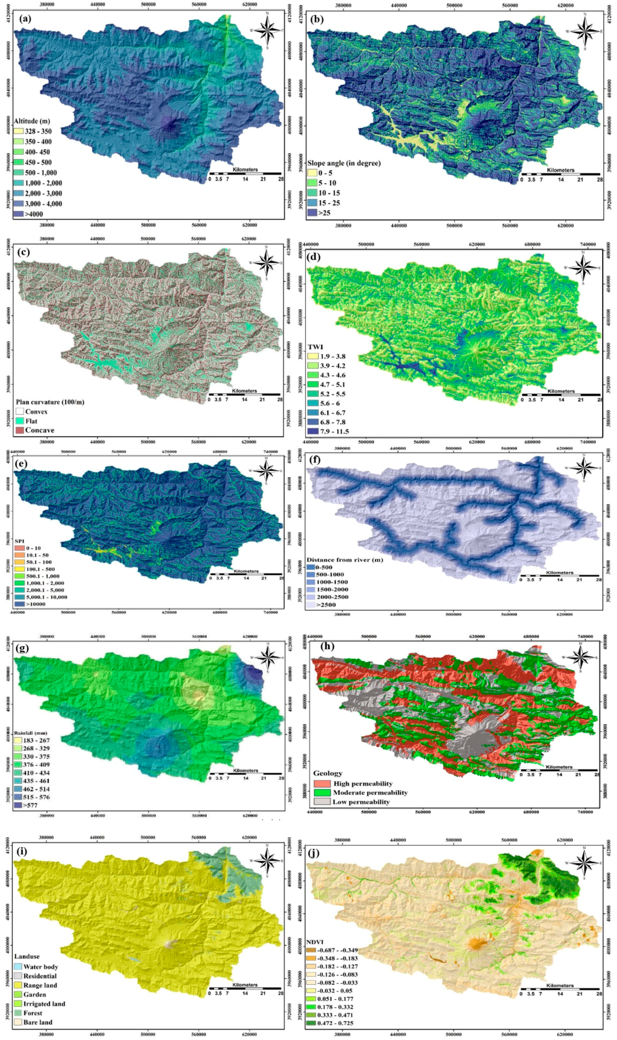
Analysis of elevation maps, as well as the position of flood points, revealed that flooding usually occurs at lower elevations. It also indicated that the frequency of recorded flooding events decreased as elevation class increased, as floods generally occur in flat, lower elevation and lower slope areas where water can coalesce. Additionally, as TWI shows wetness, meaning areas with a high TWI have saturated soil, the flood potential is higher with greater TWI values. In particular, the river and its surrounding areas maintain higher flood susceptibility than any other region, and the flood risk was shown to be reduced by increasing the distance from the river. Furthermore, rainfall depth and EBF values showed an inverse relationship; this may be because rainfall often increases at higher altitudes, although the risk of flooding significantly decreases. Overall, these results are in accordance with the results of Khosravi et al. [6,16] and Tien Bui et al. [63].

The relationship between the flood locations and lithological map depicted that least amount of flooding occurred in the areas with high permeability formations (31.062%). These formations had a high potential for saturating processes and hence allowed more infiltration than the low (37.568%) and moderate (31.369%) permeability formations with all other factors constant. The regions with volcanic rocks and low permeability allow more runoff to be transferred into streams, creating conditions where overbank can occur [23,97]. On the other hand, streams both collect water from runoff generated upland adjacent to the streams and from rainfall falling directly on them. Therefore, streams have been more susceptible to flooding in the Haraz catchment.

In terms of land use, villages close to the Haraz River, agricultural areas, such as citrus gardens, and areas with low topographic gradients are more susceptible to flooding. The results showed that most points recorded in the rangeland are close to registered residential areas and gardens; therefore, a single flood event may turn into a fatal natural hazard, causing catastrophic financial damage as well as claiming many human lives. Such devastation has been one of the leading causes of death and economic distress in the Haraz catchment, according to annual reports by authorities.

According to Park [82], the main limitation of the EBF method is that if a flood event did not happen in a represented class, the Bel and Dis results would be equal to zero, meaning that by Equation (10) the Unc or uncertainty values would be equal to 1. Walley [98] stated that if the models were provided with complete information about the study area, Pls-Bel would be expected to be equal to zero (in this case Bel is called Bayesian belief function), confirming that the two maps of Bel and Pls should have similar results [18]; which they did in this study. Furthermore, the results of this study were also consistent with other research [19,21,99,100]. According to the results of Nampak et al. [19], the main advantage of the Dempster–Shafer theory is that the application of an EBF model not only provides predictive maps of the desired area but also provides the predictive degree of uncertainty. The results of the present study were also consistent with Razavi and Malek [101], as they compared the results of the EBF method with an ensemble of AHP and EBF, finding that that EBF model has a higher prediction power than the ensemble method. Tehrany and Kumar [102] used an EBF model for flood susceptibility and compared the results with LR and FR models, similarly finding that the EBF model yielded the highest prediction power. Similarly, Arabameri at al. [28] found that EBF model had the highest prediction power over FR, TOPSIS, and VIKOR models. In contrast, Khosravi et al. [16], who applied FR and WOE models to a similar case study with similar input data, found that the FR and WOE models had slightly better prediction powers than the EBF model and its ensembles.

The current study showed that a greater number of input variables enhanced the results of modeling, which corresponded to Donati and Turrini [103], who explained that a higher number of variables would likely result in improved model accuracy. The high accuracy of the EBF model used in this study was in line with Nampak et al. [19], Pourghasemi and Beheshtirad [65], and Rahmati et al. [17]. Additionally, the developed FSMs showed that the areas nearest to the Haraz River with low slope, flat curvature, low altitude, and a high TWI were highly susceptible to flooding, which is in agreement with Tehrany et al. [13] and Khosravi et al. [6,16]. Overall, the results of the current study could be extremely useful in improving flood management and planning within the area in order to prevent and mitigate further damages due to flooding hazards. For example, by avoiding the construction of homes, villas, or industries in susceptible zones, and by employing both structural and non-structural approaches for future flood mitigation, the enduring damage and devastation caused by floods can be significantly reduced.

One of the main limitations of the current study was the use of Google Earth, rather than a field survey, for the identification of non-flooding points, though some prior researchers that had done the same, such as Tehrany et al. [15,64], Khosravi et al. [16] and Khosravi et al. [27]. Additionally, LIDAR DEM, with its high resolution, would have likely affected the results and prediction power of the models positively; thus, it is recommended that further studies employ LIDAR instead of ASTER GDEM. Further recommendations for future research include a comprehensive comparative study involving an assessment of the accuracy and simplicity of assorted bivariate, multivariate, machine learning, data mining, and multi-criteria decision-making models and their ensembles, for improving flood prediction.

Furthermore, as the current case study was in a region with diverse topography, it is recommended that future researchers examine the models’ prediction power in mountainous areas and flat areas separately, to determine which model is better for which type of topography. The main limitation of the current methodology is that the models used resulted in flood susceptibility maps (prone areas without depth, velocity, and hydraulic details) which differ from the results of 2D flood inundation models [97]. Therefore, it is recommended that future researchers compare the results of the present study with the 2D results of numerical models such as HEC-RAS. However, it should be noted that in comparison to susceptibility mapping, 1D and 2D hydraulic models are mostly performed on short river sections but not limited to any short reach and can be used for a catchment with a complicated drainage network. It is important to bear in mind that hydraulic models require different input data (e.g., design discharges with different return period, river cross sections, and roughness coefficients in main channel and flood plains) and better accuracy (e.g., high-resolution DEM and detailed topography). Therefore, combining the results of both flood inundation and susceptibility maps may offer a better outcome for decision makers in flood mitigation and management.

6. Conclusions

The main goal of this study was to assess the performance of an EBF model that is rarely used for the development of flood susceptibility maps, in comparison to an LR model and an ensemble LR EBF model, in creating FSMs for the Haraz Catchment, Iran. The LR model was implemented using independent variables that were weighted and reclassified by the EBF model. Based on the coefficients obtained from the LR model, the TWI parameter had the highest weight and thus the greatest impact on flood occurrence. The relationship between factors affecting flooding and the final maps generated by the models indicated that most flooding events occur in areas where the topography is relatively flat. The FSMs created in the current study illustrated that most flooding in the Haraz Catchment occurs in areas directly adjacent to the river, which are often characterized by low slope, and concave or flat curvature. Due to the steep, mountainous areas in the Haraz Catchment, frequent rapid runoff occurs, and water flows down toward the Haraz River, causing flash flooding in areas where topography permits. This is important as most residential and agricultural zones within this catchment are located in flat areas with low slopes, and thus were found to be especially susceptible to flooding.

According to the success-rate and prediction-rate curves, the EBF model exhibited the highest accuracy with a 94.61% success rate and 94.5% prediction rate. Alternatively, the developed EBF from LR model had an accuracy of 66.41%, which was 28.5% lower than the EBF model alone. Based on the expressed curves, the accuracy of the EBF-LR enter and stepwise models were found to be 83.19% and 52.98%, respectively; with the difference between these two models being 30.21%. The lowest accuracy belonged to the EBF-LR (stepwise) model, indicating this method is inappropriate for determining flood-prone areas. Furthermore, the results of the EBF-LR (stepwise) model suggested that altitude, slope, TWI, and distance from the river, may not be sufficient to adequately validate the model for flood susceptibility prediction. This is likely because the occurrence of a natural hazard, like flooding, is very complex and cannot be predicted with high accuracy when limited parameters are being considered in model development.

Furthermore, according to the FSM resulting from the EBF model, 15% of the total area was located in the high and very high susceptibility classes while 62% of the area was located within the low and very low susceptibility classes. Therefore, it is recommended that researchers and stakeholders identify flood-prone areas in additional catchments using the EBF model, which has a high degree of accuracy and relative simplicity. Finally, the results of this research also indicated that the impact of the different classes of the factors was more important for natural hazard assessment and mapping than the impact of the different factors themselves (i.e., the weights of the individual layers).

The developed model can now be used as a tool for decision making by management agencies such as the Department of Water and Natural Resources. The results and insights gained from this modeling effort can provide an improved understanding of flood susceptibility in the region. More generally, the results can help to improve the identification of flood-prone regions in other areas of the world. Overall, flood susceptibility mapping is essential for the prevention and mitigation of damages resulting from future floods, specifically in the northern areas of Iran. In future studies, it is recommended that researchers focus on the flood-prone areas identified in order to develop best management practices and implement structural and non-structural methods for potential damage reduction.

References

1. Youssef, A.M.; Pradhan, B.; Hassan, A.M. Flash flood risk estimation along the st. Katherine road, southern sinai, Egypt using GIS based morphometry and satellite imagery. Environ. Earth Sci. 2011, 62, 611–623. [Google Scholar] [CrossRef]
2. Grahn, T.; Nyberg, L. Assessment of pluvial flood exposure and vulnerability of residential areas. Int. J. Disaster Risk Reduct. 2017, 21, 367–375. [Google Scholar] [CrossRef]
3. Chapi, K.; Singh, V.P.; Shirzadi, A.; Shahabi, H.; Bui, D.T.; Pham, B.T.; Khosravi, K. A novel hybrid artificial intelligence approach for flood susceptibility assessment. Environ. Model. Softw. 2017, 95, 229–245. [Google Scholar] [CrossRef]
4. Bubeck, P.; Botzen, W.J.; Aerts, J.C. A review of risk perceptions and other factors that influence flood mitigation behavior. Risk Anal. Int. J. 2012, 32, 1481–1495. [Google Scholar] [CrossRef] [PubMed]
5. Shafizadeh-Moghadam, H.; Valavi, R.; Shahabi, H.; Chapi, K.; Shirzadi, A. Novel forecasting approaches using combination of machine learning and statistical models for flood susceptibility mapping. J. Environ. Manag. 2018, 217, 1–11. [Google Scholar] [CrossRef] [Green Version]
6. Khosravi, K.; Pham, B.T.; Chapi, K.; Shirzadi, A.; Shahabi, H.; Revhaug, I.; Prakash, I.; Bui, D.T. A comparative assessment of decision trees algorithms for flash flood susceptibility modeling at Haraz watershed, Northern Iran. Sci. Total Environ. 2018, 627, 744–755. [Google Scholar] [CrossRef]
7. Opolot, E. Application of remote sensing and geographical information systems in flood management: A review. Res. J. Appl. Sci. Eng. Technol. 2013, 6, 1884–1894. [Google Scholar] [CrossRef]
8. Varoonchotikul, P. Flood Forecasting Using Artificial Neural Networks; CRC Press: Boca Raton, FL, USA, 2003. [Google Scholar]
9. Levy, J.K.; Hartmann, J.; Li, K.W.; An, Y.; Asgary, A. Multi-criteria decision support systems for flood hazard mitigation and emergency response in urban watersheds 1. JAWRA J. Am. Water Resour. Assoc. 2007, 43, 346–358. [Google Scholar] [CrossRef]
10. Lee, J.-M.; Hyun, K.-H.; Choi, J.-S.; Yoon, Y.-J.; Geronimo, F.K.F. Flood reduction analysis on watershed of lid design demonstration district using swmm5. Desalin. Water Treat. 2012, 38, 255–261. [Google Scholar] [CrossRef]
11. Oh, H.-J.; Pradhan, B. Application of a neuro-fuzzy model to landslide-susceptibility mapping for shallow landslides in a tropical hilly area. Comput. Geosci. 2011, 37, 1264–1276. [Google Scholar] [CrossRef]
12. Tien Bui, D.; Shahabi, H.; Shirzadi, A.; Chapi, K.; Alizadeh, M.; Chen, W.; Mohammadi, A.; Ahmad, B.; Panahi, M.; Hong, H. Landslide detection and susceptibility mapping by AIRSAR data using support vector machine and index of entropy models in Cameron Highlands, Malaysia. Remote Sens. 2018, 10, 1527. [Google Scholar] [CrossRef]
13. Tehrany, M.S.; Pradhan, B.; Jebur, M.N. Spatial prediction of flood susceptible areas using rule based decision tree (dt) and a novel ensemble bivariate and multivariate statistical models in GIS. J. Hydrol. 2013, 504, 69–79. [Google Scholar] [CrossRef]
14. Tehrany, M.S.; Pradhan, B.; Mansor, S.; Ahmad, N. Flood susceptibility assessment using GIS-based support vector machine model with different kernel types. Catena 2015, 125, 91–101. [Google Scholar] [CrossRef]
15. Tehrany, M.S.; Pradhan, B.; Jebur, M.N. Flood susceptibility analysis and its verification using a novel ensemble support vector machine and frequency ratio method. Stoch. Environ. Res. Risk Assess. 2015, 29, 1149–1165. [Google Scholar] [CrossRef]
16. Khosravi, K.; Nohani, E.; Maroufinia, E.; Pourghasemi, H.R. A gis-based flood susceptibility assessment and its mapping in Iran: A comparison between frequency ratio and weights-of-evidence bivariate statistical models with multi-criteria decision-making technique. Nat. Hazards 2016, 83, 947–987. [Google Scholar] [CrossRef]
17. Rahmati, O.; Pourghasemi, H.R.; Zeinivand, H. Flood susceptibility mapping using frequency ratio and weights-of-evidence models in the Golastan Province, Iran. Geocarto Int. 2016, 31, 42–70. [Google Scholar] [CrossRef]
18. Althuwaynee, O.F.; Pradhan, B.; Lee, S. Application of an evidential belief function model in landslide susceptibility mapping. Comput. Geosci. 2012, 44, 120–135. [Google Scholar] [CrossRef]
19. Nampak, H.; Pradhan, B.; Manap, M.A. Application of GIS based data driven evidential belief function model to predict groundwater potential zonation. J. Hydrol. 2014, 513, 283–300. [Google Scholar] [CrossRef]
20. Tien Bui, D.; Shahabi, H.; Shirzadi, A.; Chapi, K.; Hoang, N.-D.; Pham, B.; Bui, Q.-T.; Tran, C.-T.; Panahi, M.; Bin Ahamd, B. A novel integrated approach of relevance vector machine optimized by imperialist competitive algorithm for spatial modeling of shallow landslides. Remote Sens. 2018, 10, 1538. [Google Scholar] [CrossRef]
21. Althuwaynee, O.F.; Pradhan, B.; Park, H.-J.; Lee, J.H. A novel ensemble bivariate statistical evidential belief function with knowledge-based analytical hierarchy process and multivariate statistical logistic regression for landslide susceptibility mapping. Catena 2014, 114, 21–36. [Google Scholar] [CrossRef]
22. Pradhan, B. Flood susceptible mapping and risk area delineation using logistic regression, GIS and remote sensing. J. Spat. Hydrol. 2009, 9, 1–18. [Google Scholar]
23. Haghizadeh, A.; Siahkamari, S.; Haghiabi, A.H.; Rahmati, O. Forecasting flood-prone areas using shannon’s entropy model. J. Earth Syst. Sci. 2017, 126, 39. [Google Scholar] [CrossRef]
24. Rahmati, O.; Zeinivand, H.; Besharat, M. Flood hazard zoning in Yasooj region, Iran, using GIS and multi-criteria decision analysis. Geomat. Nat. Hazards Risk 2016, 7, 1000–1017. [Google Scholar] [CrossRef]
25. Termeh, S.V.R.; Kornejady, A.; Pourghasemi, H.R.; Keesstra, S. Flood susceptibility mapping using novel ensembles of adaptive neuro fuzzy inference system and metaheuristic algorithms. Sci. Total Environ. 2018, 615, 438–451. [Google Scholar] [CrossRef] [PubMed]
26. Ahmadlou, M.; Karimi, M.; Alizadeh, S.; Shirzadi, A.; Parvinnejhad, D.; Shahabi, H.; Panahi, M. Flood susceptibility assessment using integration of adaptive network-based fuzzy inference system (ANFIS) and biogeography-based optimization (BBO) and bat algorithms (BA). Geocarto Int. 2018, 1–21. [Google Scholar] [CrossRef]
27. Khosravi, K.; Shahabi, H.; Pham, B.T.; Adamawoski, J.; Shirzadi, A.; Pradhan, B.; Dou, J.; Ly, H.-B.; Gróf, G.; Ho, H.L.; et al. A comparative assessment of flood susceptibility modeling using multi-criteria decision-making analysis and machine learning methods. J. Hydrol. 2019, 573, 311–323. [Google Scholar] [CrossRef]
28. Arabameri, A.; Rezaei, K.; Cerdà, A.; Conoscenti, C.; Kalantari, Z. A comparison of statistical methods and multi-criteria decision making to map flood Hazard susceptibility in Northern Iran. Sci. Total Environ. 2019, 660, 443–458. [Google Scholar] [CrossRef]
29. Chen, W.; Shirzadi, A.; Shahabi, H.; Ahmad, B.B.; Zhang, S.; Hong, H.; Zhang, N. A novel hybrid artificial intelligence approach based on the rotation forest ensemble and naïve bayes tree classifiers for a landslide susceptibility assessment in Langao County, China. Geomat. Nat. Hazards Risk 2017, 8, 1955–1977. [Google Scholar] [CrossRef]
30. Chen, W.; Shahabi, H.; Shirzadi, A.; Li, T.; Guo, C.; Hong, H.; Li, W.; Pan, D.; Hui, J.; Ma, M. A novel ensemble approach of bivariate statistical-based logistic model tree classifier for landslide susceptibility assessment. Geocarto Int. 2018, 33, 1398–1420. [Google Scholar] [CrossRef]
31. Pham, B.T.; Shirzadi, A.; Bui, D.T.; Prakash, I.; Dholakia, M. A hybrid machine learning ensemble approach based on a radial basis function neural network and rotation forest for landslide susceptibility modeling: A case study in the Himalayan area, India. Int. J. Sediment. Res. 2018, 33, 157–170. [Google Scholar] [CrossRef]
32. Abedini, M.; Ghasemian, B.; Shirzadi, A.; Shahabi, H.; Chapi, K.; Pham, B.T.; Bin Ahmad, B.; Tien Bui, D. A novel hybrid approach of bayesian logistic regression and its ensembles for landslide susceptibility assessment. Geocarto Int. 2018, 1–31. [Google Scholar] [CrossRef]
33. Jaafari, A.; Panahi, M.; Pham, B.T.; Shahabi, H.; Bui, D.T.; Rezaie, F.; Lee, S. Meta optimization of an adaptive neuro-fuzzy inference system with grey wolf optimizer and biogeography-based optimization algorithms for spatial prediction of landslide susceptibility. Catena 2019, 175, 430–445. [Google Scholar] [CrossRef]
34. Nguyen, V.V.; Pham, B.T.; Vu, B.T.; Prakash, I.; Jha, S.; Shahabi, H.; Shirzadi, A.; Ba, D.N.; Kumar, R.; Chatterjee, J.M. Hybrid machine learning approaches for landslide susceptibility modeling. Forests 2019, 10, 157. [Google Scholar] [CrossRef]
35. Tien Bui, D.; Shahabi, H.; Omidvar, E.; Shirzadi, A.; Geertsema, M.; Clague, J.J.; Khosravi, K.; Pradhan, B.; Pham, B.T.; Chapi, K. Shallow landslide prediction using a novel hybrid functional machine learning algorithm. Remote Sens. 2019, 11, 931. [Google Scholar] [CrossRef]
36. Zhang, T.; Han, L.; Chen, W.; Shahabi, H. Hybrid integration approach of entropy with logistic regression and support vector machine for landslide susceptibility modeling. Entropy 2018, 20, 884. [Google Scholar] [CrossRef]
37. Chen, W.; Shahabi, H.; Zhang, S.; Khosravi, K.; Shirzadi, A.; Chapi, K.; Pham, B.; Zhang, T.; Zhang, L.; Chai, H. Landslide susceptibility modeling based on GIS and novel bagging-based kernel logistic regression. Appl. Sci. 2018, 8, 2540. [Google Scholar] [CrossRef]
38. Chen, W.; Peng, J.; Hong, H.; Shahabi, H.; Pradhan, B.; Liu, J.; Zhu, A.-X.; Pei, X.; Duan, Z. Landslide susceptibility modelling using GIS-based machine learning techniques for Chongren County, Jiangxi province, China. Sci. Total Environ. 2018, 626, 1121–1135. [Google Scholar] [CrossRef] [PubMed]
39. Chen, W.; Shahabi, H.; Shirzadi, A.; Hong, H.; Akgun, A.; Tian, Y.; Liu, J.; Zhu, A.-X.; Li, S. Novel hybrid artificial intelligence approach of bivariate statistical-methods-based kernel logistic regression classifier for landslide susceptibility modeling. Bull. Eng. Geol. Environ. 2018, 1–23. [Google Scholar] [CrossRef]
40. Shadman Roodposhti, M.; Aryal, J.; Shahabi, H.; Safarrad, T. Fuzzy shannon entropy: A hybrid GIS-based landslide susceptibility mapping method. Entropy 2016, 18, 343. [Google Scholar] [CrossRef]
41. Pham, B.T.; Prakash, I.; Khosravi, K.; Chapi, K.; Trinh, P.T.; Ngo, T.Q.; Hosseini, S.V.; Bui, D.T. A comparison of support vector machines and bayesian algorithms for landslide susceptibility modelling. Geocarto Int. 2018, 1–23. [Google Scholar] [CrossRef]
42. Shirzadi, A.; Solaimani, K.; Roshan, M.H.; Kavian, A.; Chapi, K.; Shahabi, H.; Keesstra, S.; Ahmad, B.B.; Bui, D.T. Uncertainties of prediction accuracy in shallow landslide modeling: Sample size and raster resolution. Catena 2019, 178, 172–188. [Google Scholar] [CrossRef]
43. He, Q.; Shahabi, H.; Shirzadi, A.; Li, S.; Chen, W.; Wang, N.; Chai, H.; Bian, H.; Ma, J.; Chen, Y. Landslide spatial modelling using novel bivariate statistical based naïve bayes, RBF classifier, and RBF network machine learning algorithms. Sci. Total Environ. 2019, 663, 1–15. [Google Scholar] [CrossRef]
44. Hong, H.; Shahabi, H.; Shirzadi, A.; Chen, W.; Chapi, K.; Ahmad, B.B.; Roodposhti, M.S.; Hesar, A.Y.; Tian, Y.; Bui, D.T. Landslide susceptibility assessment at the Wuning area, China: A comparison between multi-criteria decision making, bivariate statistical and machine learning methods. Nat. Hazards 2019, 96, 173–212. [Google Scholar] [CrossRef]
45. Chen, W.; Panahi, M.; Tsangaratos, P.; Shahabi, H.; Ilia, I.; Panahi, S.; Li, S.; Jaafari, A.; Ahmad, B.B. Applying population-based evolutionary algorithms and a neuro-fuzzy system for modeling landslide susceptibility. Catena 2019, 172, 212–231. [Google Scholar] [CrossRef]
46. Chen, W.; Zhang, S.; Li, R.; Shahabi, H. Performance evaluation of the GIS-based data mining techniques of best-first decision tree, random forest, and naïve bayes tree for landslide susceptibility modeling. Sci. Total Environ. 2018, 644, 1006–1018. [Google Scholar] [CrossRef] [PubMed]
47. Shirzadi, A.; Soliamani, K.; Habibnejhad, M.; Kavian, A.; Chapi, K.; Shahabi, H.; Chen, W.; Khosravi, K.; Thai Pham, B.; Pradhan, B. Novel GIS based machine learning algorithms for shallow landslide susceptibility mapping. Sensors 2018, 18, 3777. [Google Scholar] [CrossRef]
48. Shirzadi, A.; Shahabi, H.; Chapi, K.; Bui, D.T.; Pham, B.T.; Shahedi, K.; Ahmad, B.B. A comparative study between popular statistical and machine learning methods for simulating volume of landslides. Catena 2017, 157, 213–226. [Google Scholar] [CrossRef]
49. Shahabi, H.; Hashim, M. Landslide susceptibility mapping using GIS-based statistical models and remote sensing data in tropical environment. Sci. Rep. 2015, 5, 9899. [Google Scholar] [CrossRef]
50. Jaafari, A.; Zenner, E.K.; Panahi, M.; Shahabi, H. Hybrid artificial intelligence models based on a neuro-fuzzy system and metaheuristic optimization algorithms for spatial prediction of wildfire probability. Agric. Meteorol. 2019, 266, 198–207. [Google Scholar] [CrossRef]
51. Taheri, K.; Shahabi, H.; Chapi, K.; Shirzadi, A.; Gutiérrez, F.; Khosravi, K. Sinkhole susceptibility mapping: A comparison between bayes-based machine learning algorithms. Land Degrad. Dev. 2019, 30, 730–745. [Google Scholar] [CrossRef]
52. Roodposhti, M.S.; Safarrad, T.; Shahabi, H. Drought sensitivity mapping using two one-class support vector machine algorithms. Atmos. Res. 2017, 193, 73–82. [Google Scholar] [CrossRef]
53. Azareh, A.; Rahmati, O.; Rafiei-Sardooi, E.; Sankey, J.B.; Lee, S.; Shahabi, H.; Ahmad, B.B. Modelling gully-erosion susceptibility in a semi-arid region, Iran: Investigation of applicability of certainty factor and maximum entropy models. Sci. Total Environ. 2019, 655, 684–696. [Google Scholar] [CrossRef] [PubMed]
54. Tien Bui, D.; Shirzadi, A.; Shahabi, H.; Chapi, K.; Omidavr, E.; Pham, B.T.; Talebpour Asl, D.; Khaledian, H.; Pradhan, B.; Panahi, M. A novel ensemble artificial intelligence approach for gully erosion mapping in a semi-arid watershed (Iran). Sensors 2019, 19, 2444. [Google Scholar] [CrossRef] [PubMed]
55. Miraki, S.; Zanganeh, S.H.; Chapi, K.; Singh, V.P.; Shirzadi, A.; Shahabi, H.; Pham, B.T. Mapping groundwater potential using a novel hybrid intelligence approach. Water Resour. Manag. 2019, 33, 281–302. [Google Scholar] [CrossRef]
56. Rahmati, O.; Naghibi, S.A.; Shahabi, H.; Bui, D.T.; Pradhan, B.; Azareh, A.; Rafiei-Sardooi, E.; Samani, A.N.; Melesse, A.M. Groundwater spring potential modelling: Comprising the capability and robustness of three different modeling approaches. J. Hydrol. 2018, 565, 248–261. [Google Scholar] [CrossRef]
57. Khosravi, K.; Panahi, M.; Tien Bui, D. Spatial prediction of groundwater spring potential mapping based on adaptive neuro-fuzzy inference system and metaheuristic optimization. Hydrol. Earth Syst. Sci. 2018, 22, 4771–4792. [Google Scholar] [CrossRef]
58. Pham, B.T.; Prakash, I.; Singh, S.K.; Shirzadi, A.; Shahabi, H.; Bui, D.T. Landslide susceptibility modeling using reduced error pruning trees and different ensemble techniques: Hybrid machine learning approaches. CATENA 2019, 175, 203–218. [Google Scholar] [CrossRef]
59. Pradhan, B.; Abokharima, M.H.; Jebur, M.N.; Tehrany, M.S. Land subsidence susceptibility mapping at Kinta valley (Malaysia) using the evidential belief function model in GIS. Nat. Hazards 2014, 73, 1019–1042. [Google Scholar] [CrossRef]
60. Chen, W.; Pradhan, B.; Li, S.; Shahabi, H.; Rizeei, H.M.; Hou, E.; Wang, S. Novel hybrid integration approach of bagging-based fisher’s linear discriminant function for groundwater potential analysis. Nat. Resour. Res. 2019, 1–20. [Google Scholar] [CrossRef]
61. Sadeghi-Pouya, A.; Nouri, J.; Mansouri, N.; Kia-Lashaki, A. An indexing approach to assess flood vulnerability in the western coastal cities of Mazandaran, Iran. Int. J. Disaster Risk Reduct. 2017, 22, 304–316. [Google Scholar] [CrossRef]
62. Manandhar, B.; Balla, M.K.; Awal, R.; Pradhan, B.M. Floodplain Analysis and Risk Assessment of Lothar Khola (Stream). In Proceedings of the 11th ESRI India User Conference, Noida, India, 21–22 April 2010. [Google Scholar]
63. Merz, B.; Thieken, A.; Gocht, M. Flood Risk Mapping at the Local Scale: Concepts and Challenges. In Flood Risk Management in Europe; Springer: Dordrecht, The Netherlands, 2007; pp. 231–251. [Google Scholar]
64. Tehrany, M.S.; Pradhan, B.; Jebur, M.N. Flood susceptibility mapping using a novel ensemble weights-of-evidence and support vector machine models in GIS. J. Hydrol. 2014, 512, 332–343. [Google Scholar] [CrossRef]
65. Pourghasemi, H.R.; Beheshtirad, M. Assessment of a data-driven evidential belief function model and GIS for groundwater potential mapping in the Koohrang watershed, Iran. Geocarto Int. 2015, 30, 662–685. [Google Scholar] [CrossRef]
66. O’brien, R.M. A caution regarding rules of thumb for variance inflation factors. Qual. Quant. 2007, 41, 673–690. [Google Scholar] [CrossRef]
67. Yalcin, A.; Reis, S.; Aydinoglu, A.; Yomralioglu, T. A GIS-based comparative study of frequency ratio, analytical hierarchy process, bivariate statistics and logistics regression methods for landslide susceptibility mapping in Trabzon, NE Turkey. Catena 2011, 85, 274–287. [Google Scholar] [CrossRef]
68. Bednarik, M.; Magulová, B.; Matys, M.; Marschalko, M. Landslide susceptibility assessment of the Kraľovany–liptovský Mikuláš railway case study. Phys. Chem. Earthparts A/B/C 2010, 35, 162–171. [Google Scholar] [CrossRef]
69. Gokceoglu, C.; Sonmez, H.; Nefeslioglu, H.A.; Duman, T.Y.; Can, T. The 17 march 2005 kuzulu landslide (Sivas, Turkey) and landslide-susceptibility map of its near vicinity. Eng. Geol. 2005, 81, 65–83. [Google Scholar] [CrossRef]
70. Moore, I.D.; Grayson, R.; Ladson, A. Digital terrain modelling: A review of hydrological, geomorphological, and biological applications. Hydrol. Process. 1991, 5, 3–30. [Google Scholar] [CrossRef]
71. Glenn, E.P.; Morino, K.; Nagler, P.L.; Murray, R.S.; Pearlstein, S.; Hultine, K.R. Roles of saltcedar (tamarix spp.) and capillary rise in salinizing a non-flooding terrace on a flow-regulated desert river. J. Arid Environ. 2012, 79, 56–65. [Google Scholar] [CrossRef]
72. Kia, M.B.; Pirasteh, S.; Pradhan, B.; Mahmud, A.R.; Sulaiman, W.N.A.; Moradi, A. An artificial neural network model for flood simulation using GIS: Johor river Basin, Malaysia. Environ. Earth Sci. 2012, 67, 251–264. [Google Scholar] [CrossRef]
73. Tehrany, M.S.; Lee, M.-J.; Pradhan, B.; Jebur, M.N.; Lee, S. Flood susceptibility mapping using integrated bivariate and multivariate statistical models. Environ. Earth Sci. 2014, 72, 4001–4015. [Google Scholar] [CrossRef]
74. Çelik, H.E.; Coskun, G.; Cigizoglu, H.K.; Ağıralioğlu, N.; Aydın, A.; Esin, A.I. The analysis of 2004 flood on Kozdere stream in Istanbul. Nat. Hazards 2012, 63, 461–477. [Google Scholar] [CrossRef]
75. Srivastava, O.S.; Denis, D.; Srivastava, S.K.; Kumar, M.; Kumar, N. Morphometric analysis of a semi urban watershed, Trans Yamuna, draining at allahabad using cartosat (DEM) data and GIS. Int. J. Eng. Sci. (Ijes) 2014, 3, 71–79. [Google Scholar]
76. Mongelli, G.; Salvemini, A. Caratterizzazione Geolitologica e Carta della Permeabilità Della Puglia Settentrionale; Dipartimento di Ingegneria e Fisica Dell’Ambiente e Gruppo Nazionale per la Difesa dalle Catastrofi Idrogeologiche, Univ. della Basilicata, Potenza: Sicily, Italy, 14 October 1994. [Google Scholar]
77. Bui, D.T.; Panahi, M.; Shahabi, H.; Singh, V.P.; Shirzadi, A.; Chapi, K.; Khosravi, K.; Chen, W.; Panahi, S.; Li, S. Novel hybrid evolutionary algorithms for spatial prediction of floods. Sci. Rep. 2018, 8, 15364. [Google Scholar] [CrossRef] [PubMed]
78. Shahabi, H.; Ahmad, B.B.; Mokhtari, M.H.; Zadeh, M.A. Detection of urban irregular development and green space destruction using normalized difference vegetation index (NDVI), principal component analysis (PCA) and post classification methods: A case study of Saqqez city. Int. J. Phys. Sci. 2012, 7, 2587–2595. [Google Scholar]
79. Tien Bui, D.; Khosravi, K.; Li, S.; Shahabi, H.; Panahi, M.; Singh, V.; Chapi, K.; Shirzadi, A.; Panahi, S.; Chen, W. New hybrids of anfis with several optimization algorithms for flood susceptibility modeling. Water 2018, 10, 1210. [Google Scholar] [CrossRef]
80. Dempster, A.P. Upper and lower probability inferences for families of hypotheses with monotone density ratios. Ann. Math. Stat. 1969, 40, 953–969. [Google Scholar] [CrossRef]
81. Shafer, G. A Mathematical Theory of Evidence; Princeton University Press: Princeton, NJ, USA, 1976; Volume 42. [Google Scholar]
82. Park, N.-W. Application of dempster-shafer theory of evidence to GIS-based landslide susceptibility analysis. Environ. Earth Sci. 2011, 62, 367–376. [Google Scholar] [CrossRef]
83. Carranza, E.J.M.; Hale, M. Evidential belief functions for data-driven geologically constrained mapping of gold potential, Pbaguio district, Philippines. Ore Geol. Rev. 2003, 22, 117–132. [Google Scholar] [CrossRef]
84. Chen, W.; Zhao, X.; Shahabi, H.; Shirzadi, A.; Khosravi, K.; Chai, H.; Zhang, S.; Zhang, L.; Ma, J.; Chen, Y. Spatial prediction of landslide susceptibility by combining evidential belief function, logistic regression and logistic model tree. Geocarto Int. 2019, 1–25. [Google Scholar] [CrossRef]
85. Shirzadi, A.; Saro, L.; Joo, O.H.; Chapi, K. A GIS-based logistic regression model in rock-fall susceptibility mapping along a mountainous road: Salavat Abad case study, Kurdistan, Iran. Nat. Hazards 2012, 64, 1639–1656. [Google Scholar] [CrossRef] [Green Version]
86. Shahabi, H.; Khezri, S.; Ahmad, B.B.; Hashim, M. Landslide susceptibility mapping at central zab basin, Iran: A comparison between analytical hierarchy process, frequency ratio and logistic regression models. Catena 2014, 115, 55–70. [Google Scholar] [CrossRef]
87. Umar, Z.; Pradhan, B.; Ahmad, A.; Jebur, M.N.; Tehrany, M.S. Earthquake induced landslide susceptibility mapping using an integrated ensemble frequency ratio and logistic regression models in west Sumatera province, Indonesia. Catena 2014, 118, 124–135. [Google Scholar] [CrossRef]
88. Hosmer, D.W.; Lemeshow, S. Applied Logistic Regression.(sl); Wiley: Hoboken, NJ, USA, 2000. [Google Scholar]
89. Papadopoulou-Vrynioti, K.; Bathrellos, G.D.; Skilodimou, H.D.; Kaviris, G.; Makropoulos, K. Karst collapse susceptibility mapping considering peak ground acceleration in a rapidly growing urban area. Eng. Geol. 2013, 158, 77–88. [Google Scholar] [CrossRef]
90. Pourghasemi, H.R.; Mohammady, M.; Pradhan, B. Landslide susceptibility mapping using index of entropy and conditional probability models in GIS: Safarood basin, Iran. Catena 2012, 97, 71–84. [Google Scholar] [CrossRef]
91. Chung, C.-J.F.; Fabbri, A.G. Validation of spatial prediction models for landslide hazard mapping. Nat. Hazards 2003, 30, 451–472. [Google Scholar] [CrossRef]
92. Bui, D.T.; Pradhan, B.; Lofman, O.; Revhaug, I.; Dick, O.B. Landslide susceptibility mapping at Hoa Binh province (Vietnam) using an adaptive neuro-fuzzy inference system and gis. Comput. Geosci. 2012, 45, 199–211. [Google Scholar]
93. Pradhan, B. A comparative study on the predictive ability of the decision tree, support vector machine and neuro-fuzzy models in landslide susceptibility mapping using GIS. Comput. Geosci. 2013, 51, 350–365. [Google Scholar] [CrossRef]
94. Brenning, A. Spatial prediction models for landslide hazards: Review, comparison and evaluation. Nat. Hazards Earth Syst. Sci. 2005, 5, 853–862. [Google Scholar] [CrossRef]
95. Bui, D.T.; Lofman, O.; Revhaug, I.; Dick, O. Landslide susceptibility analysis in the Hoa Binh province of Vietnam using statistical index and logistic regression. Nat. Hazards 2011, 59, 1413. [Google Scholar] [CrossRef]
96. Maier, H.R.; Dandy, G.C. Neural networks for the prediction and forecasting of water resources variables: A review of modelling issues and applications. Environ. Model. Softw. 2000, 15, 101–124. [Google Scholar] [CrossRef]
97. Chen, W.; Hong, H.; Li, S.; Shahabi, H.; Wang, Y.; Wang, X.; Ahmad, B.B. Flood susceptibility modelling using novel hybrid approach of reduced-error pruning trees with bagging and random subspace ensembles. J. Hydrol. 2019, 575, 864–873. [Google Scholar] [CrossRef]
98. Walley, P. Belief function representations of statistical evidence. Ann. Stat. 1987, 15, 1439–1465. [Google Scholar] [CrossRef]
99. Carranza, E.J.M.; Van Ruitenbeek, F.; Hecker, C.; van der Meijde, M.; van der Meer, F.D. Knowledge-guided data-driven evidential belief modeling of mineral prospectivity in Cabo De Gata, SE Spain. Int. J. Appl. Earth Obs. Geoinf. 2008, 10, 374–387. [Google Scholar] [CrossRef]
100. Bui, D.T.; Pradhan, B.; Lofman, O.; Revhaug, I.; Dick, O.B. Spatial prediction of landslide hazards in Hoa Binh province (Vietnam): A comparative assessment of the efficacy of evidential belief functions and fuzzy logic models. Catena 2012, 96, 28–40. [Google Scholar]
101. Razavi Termeh, V.; Malek, M. Flood susceptibility mapping using ensemble of evidential belief (EBF) function with analytical hierarchy process (AHP) (Case study: Jhrom township). Geospat. Eng. J. 2017, 8, 1–15. [Google Scholar]
102. Tehrany, M.S.; Kumar, L. The application of a dempster–shafer-based evidential belief function in flood susceptibility mapping and comparison with frequency ratio and logistic regression methods. Environ. Earth Sci. 2018, 77, 490. [Google Scholar] [CrossRef]
103. Donati, L.; Turrini, M. An objective method to rank the importance of the factors predisposing to landslides with the GIS methodology: Application to an area of the Apennines (Valnerina; Perugia, Italy). Eng. Geol. 2002, 63, 277–289. [Google Scholar] [CrossRef]
Figure 1. Flood locations mapped on a hill-shaded map of the Haraz Catchment, Iran.
Remotesensing 11 01589 g001
Figure 2. (a) Flood in Surkh Rod and Mahmoud Abad, on April 12, 2015, (b) flood in Neka on September 12, 2012, (c) flood in Behshahr on September 16, 2013.
Remotesensing 11 01589 g002
Figure 3. Flood-conditioning factors of the study area: (a) Altitude (m), (b) Slope angle (In degrees), (c) plan curvature (100/m), (d) topographic wetness index (TWI), (e) Stream power index (SPI), (f) distance from river (m), (g) rainfall (mm), (h) geology, (i) land use, and (j) NDVI.
Remotesensing 11 01589 g003
Figure 4. Flow chart of the adopted research methodology used to create flood susceptibility maps of the Haraz Catchment.
Remotesensing 11 01589 g004
Figure 5. Integrated results of EBF model: (a) belief (Bel), (b) disbelief (Dis), (c) uncertainty (Unc), (d) plausibility (Pls).
Remotesensing 11 01589 g005
Figure 6. Flood Susceptibility Index using (a) EBF, (b) EBF-LR (Enter), (c) EBF-LR (Stepwise), (d) EBF from LR.
Remotesensing 11 01589 g006
Figure 7. The success and prediction-rate curves for flooding map; (a) success rate and (b) prediction rate.
Remotesensing 11 01589 g007
Figure 8. A histogram showing the percentage of flood zones that fall into the various classes from the four models.
Remotesensing 11 01589 g008