Optimization of X-Band Radar Rainfall Retrieval in the Southern Andes of Ecuador Using a Random Forest Model


Abstract
:1. Introduction
2. Materials and Methods
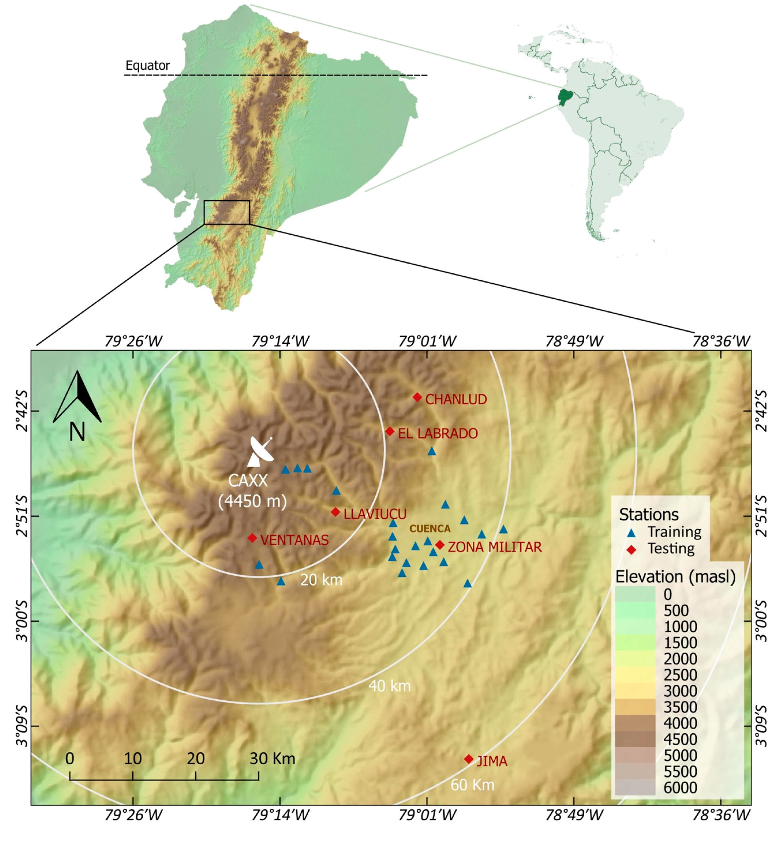
2.1. Study Site
2.2. Instruments and Data
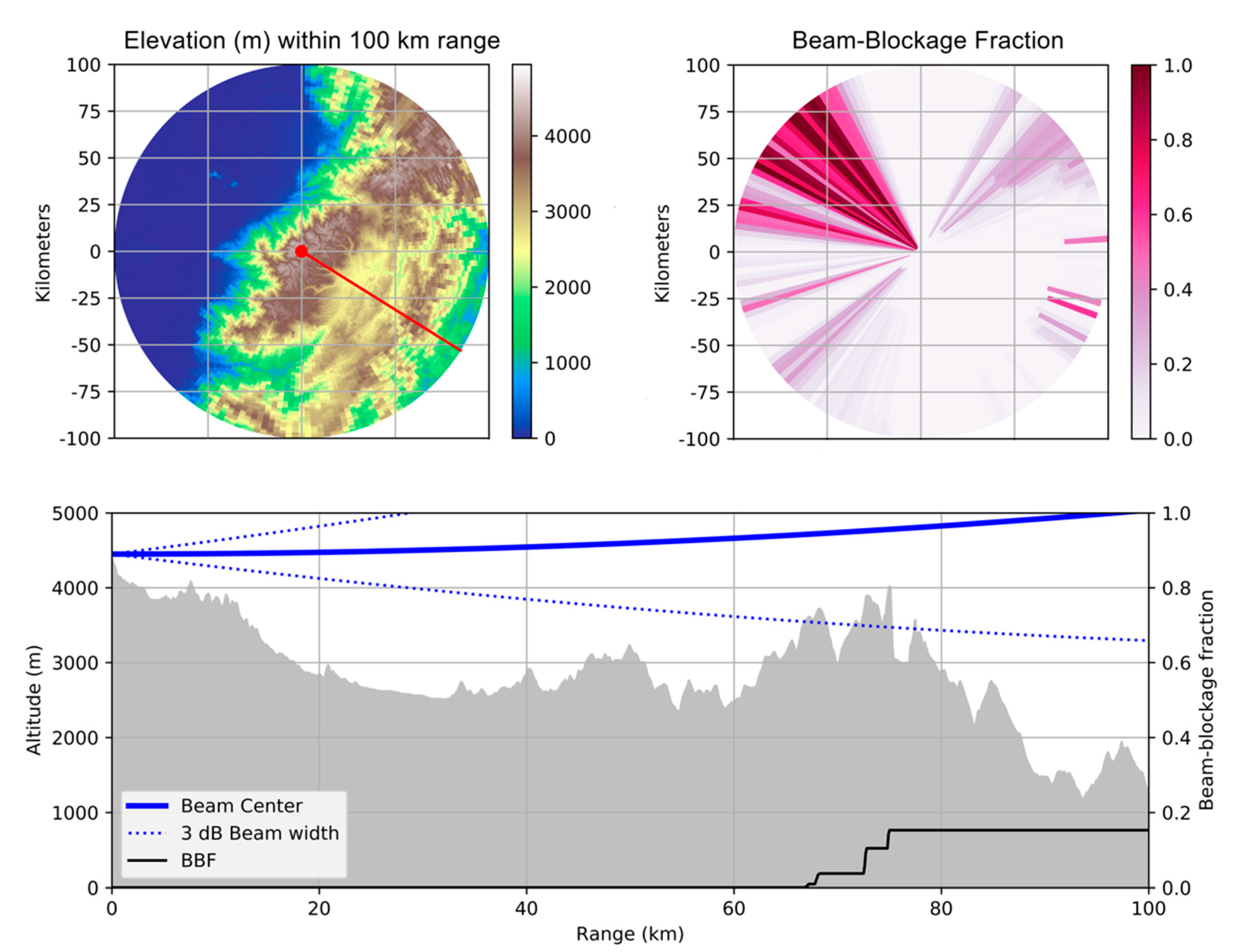
2.2.1. Radar
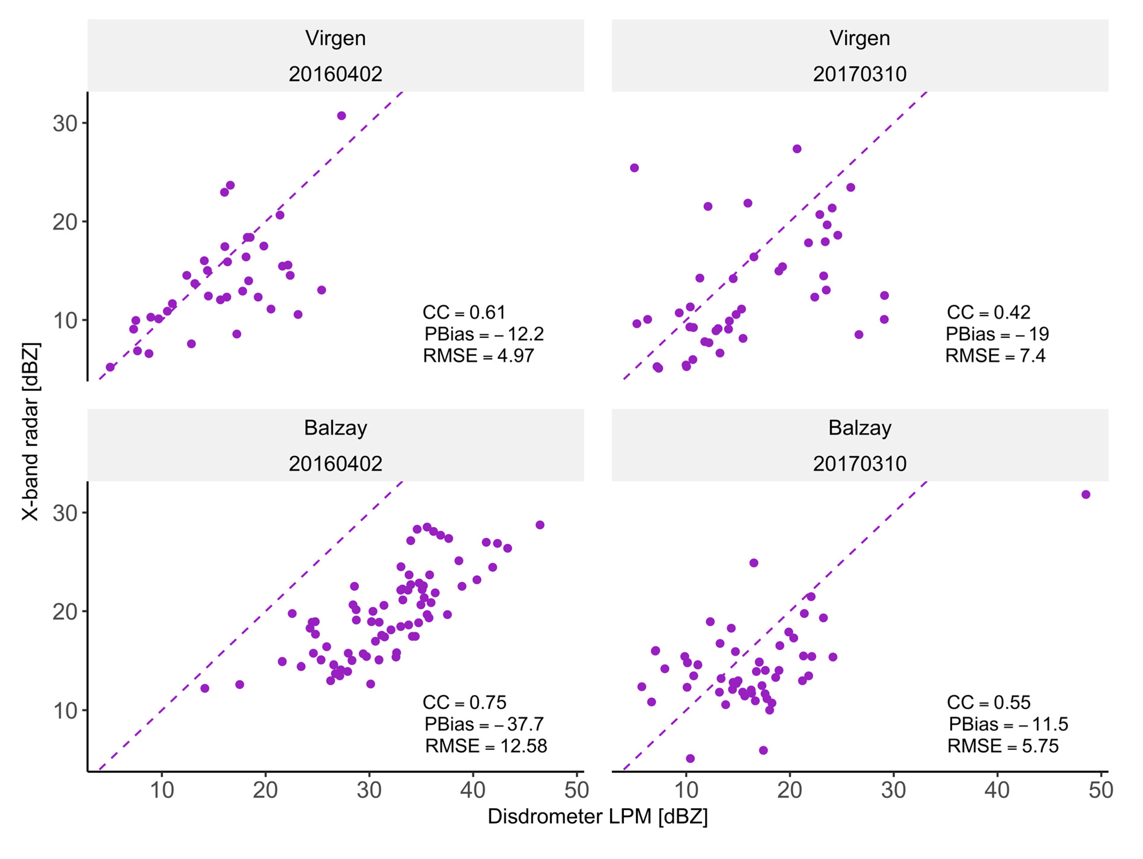
2.2.2. Disdrometers
2.2.3. Rain Gauges
2.3. QPE Models
Step-Wise Correction Model
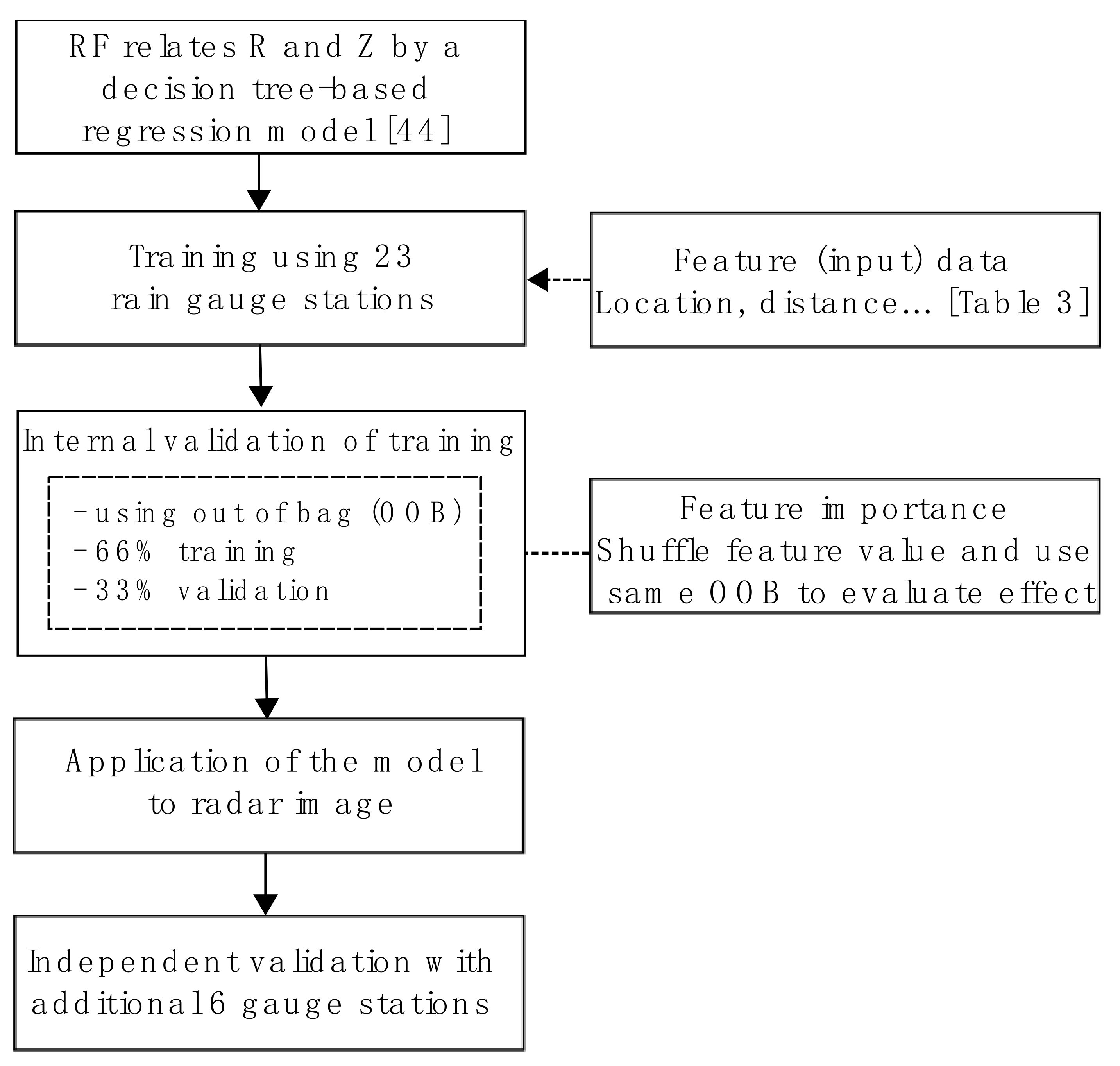
2.4. Random Forest Model
Input Features
2.5. Evaluation
3. Analysis and Discussion
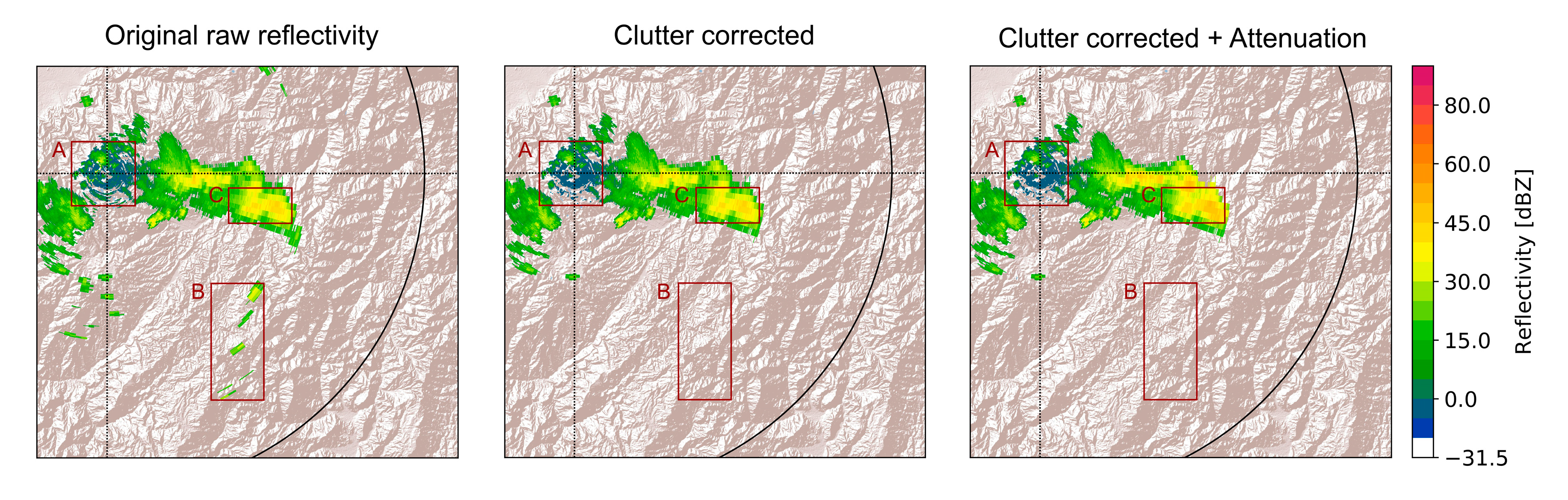
3.1. Step-Wise Correction Model
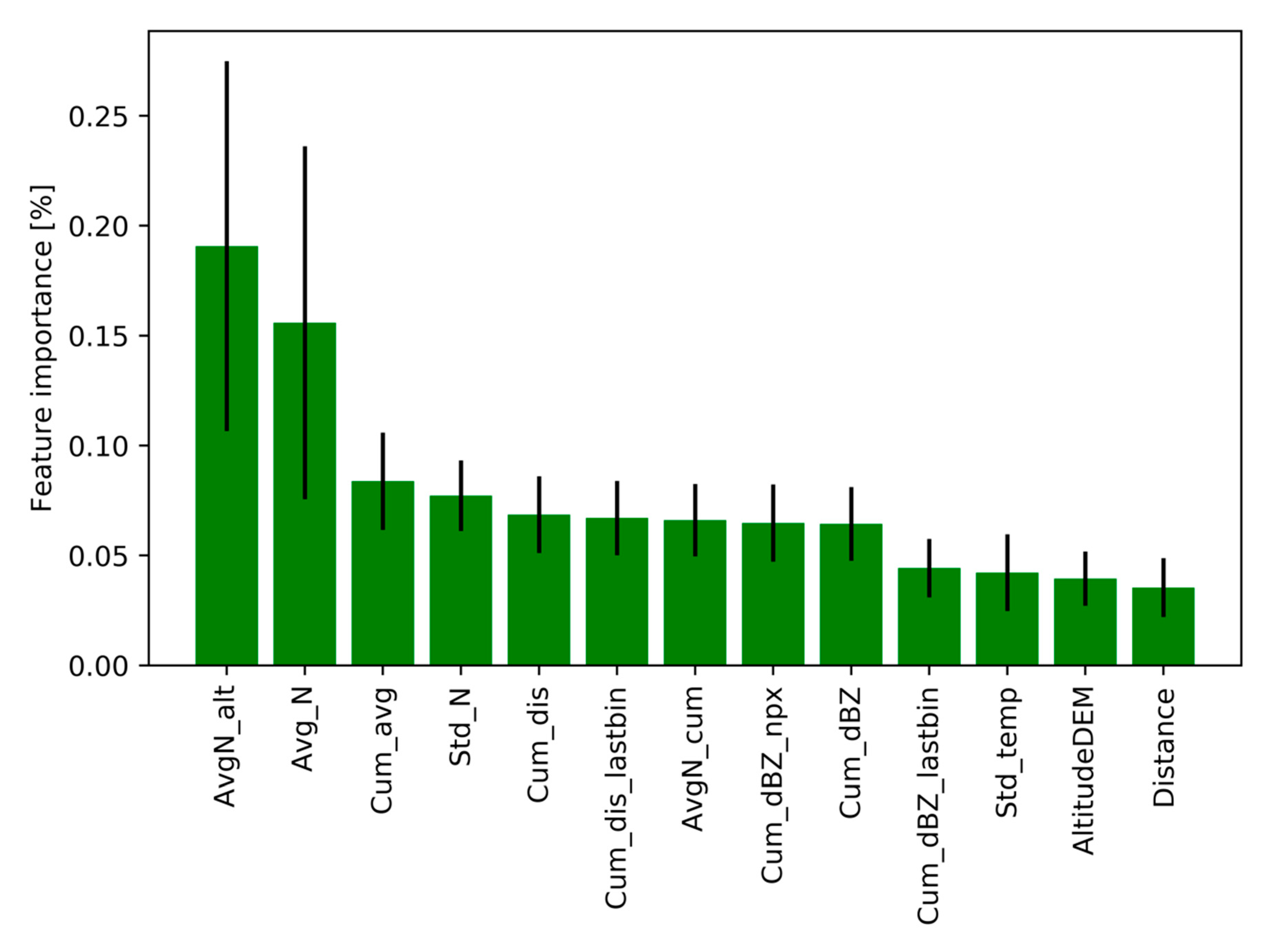
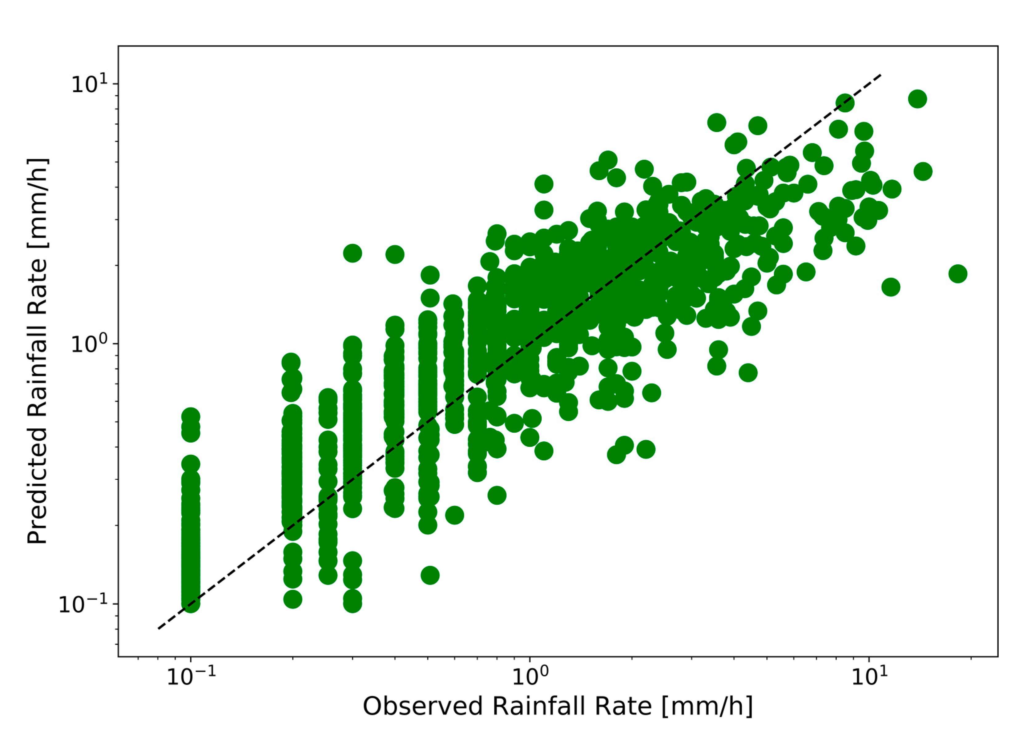
3.2. Random Forest Model
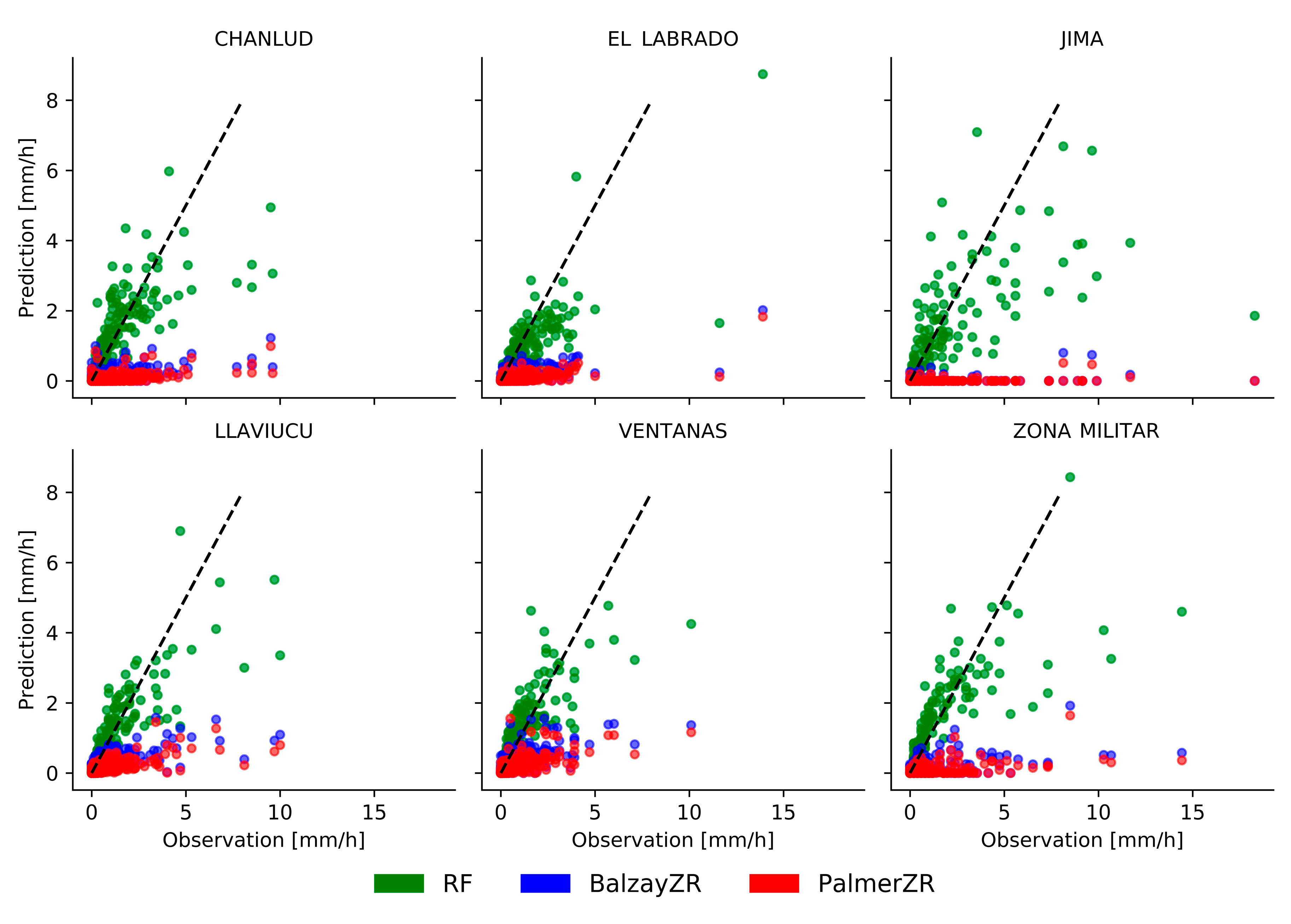
3.3. Comparison of the Models - Temporal and Spatial Evaluation
4. Conclusions
Author Contributions
Funding
Acknowledgments
Conflicts of Interest
Abbreviations
| QPE | Quantitative Precipitation Estimation |
| RF | Random forest |
| ANN | Artificial Neural Networks |
| PPI | Plan Position Indicator |
| MSE | Mean square error |
References
- Orellana-Alvear, J.; Célleri, R.; Rollenbeck, R.; Bendix, J. Analysis of Rain Types and Their Z–R Relationships at Different Locations in the High Andes of Southern Ecuador. J. Appl. Meteorol. Climatol. 2017, 56, 3065–3080. [Google Scholar] [CrossRef]
- Anagnostou, M.N.; Nikolopoulos, E.I.; Kalogiros, J.; Anagnostou, E.N.; Marra, F.; Mair, E.; Bertoldi, G.; Tappeiner, U.; Borga, M. Advancing precipitation estimation and streamflow simulations in complex terrain with X-Band dual-polarization radar observations. Remote Sens. 2018, 10. [Google Scholar] [CrossRef]
- Kirstetter, P.E.; Gourley, J.J.; Hong, Y.; Zhang, J.; Moazamigoodarzi, S.; Langston, C.; Arthur, A. Probabilistic precipitation rate estimates with ground-based radar networks. Water Resour. Res. 2015, 51, 1422–1442. [Google Scholar] [CrossRef]
- Büyükbas, E. Assess the Current and Potential Capabilities of Weather Radars for the Use in WMO Integrated Global Observing System (WIGOS). In Proceedings of the Joint Meeting of the CIMO Expert Team on Remote Sensing Upper-air Technology and Techniques and CBS Expert Team on Surface Based Remote Sensing, Geneva, Switzerland, 23–27 November 2009. [Google Scholar]
- McLaughlin, D.; Pepyne, D.; Chandrasekar, V.; Philips, B.; Kurose, J.; Zink, M.; Droegemeier, K.; Cruz-Pol, S.; Junyent, F.; Brotzge, J.; et al. Short-wavelength technology and the potential for distributed networks of small radar systems. Bull. Am. Meteorol. Soc. 2009, 1797–1817. [Google Scholar] [CrossRef]
- Mishra, K.V.; Krajewski, W.F.; Goska, R.; Ceynar, D.; Seo, B.C.; Kruger, A.; Niemeier, J.J.; Galvez, P.A.; Thurai, M.; Bringi, V.N.; et al. Deployment and Performance Analyses of High-Resolution Iowa XPOL Radar System during the NASA IFloodS Campaign. J. Hydrometeorol. 2016, 17, 455–479. [Google Scholar] [CrossRef]
- Feng, L.; Xiao, H.; Wen, G.; Li, Z.; Sun, Y.; Tang, Q.; Liu, Y. Rain Attenuation Correction of Reflectivity for X-Band Dual Polarization Radar. Atmosphere 2016, 7, 164. [Google Scholar] [CrossRef]
- Diederich, M.; Ryzhkov, A.; Simmer, C.; Zhang, P.; Trömel, S. Use of Specific Attenuation for Rainfall Measurement at X-Band Radar Wavelengths. Part II: Rainfall Estimates and Comparison with Rain Gauges. J. Hydrometeorol. 2015, 16, 503–516. [Google Scholar] [CrossRef]
- Villarini, G.; Krajewski, W.F. Review of the different sources of uncertainty in single polarization radar-based estimates of rainfall. Surv. Geophys. 2010, 31, 107–129. [Google Scholar] [CrossRef]
- Antonini, A.; Melani, S.; Corongiu, M.; Romanelli, S.; Mazza, A.; Ortolani, A.; Gozzini, B. On the Implementation of a regional X-bandweather radar network. Atmosphere 2017, 8, 25. [Google Scholar] [CrossRef]
- Lo Conti, F.; Francipane, A.; Pumo, D.; Noto, L.V. Exploring single polarization X-band weather radar potentials for local meteorological and hydrological applications. J. Hydrol. 2015, 531, 508–522. [Google Scholar] [CrossRef]
- Allegretti, M. X-Band Mini Radar for Observing and Monitoring Rainfall Events. Atmos. Clim. Sci. 2012, 2, 290–297. [Google Scholar] [CrossRef]
- Bendix, J.; Fries, A.; Zárate, J.; Trachte, K.; Rollenbeck, R.; Pucha-Cofrfrep, F.; Paladines, R.; Palacios, I.; Orellana, J.; Oñate-Valdivieso, F.; et al. RadarNet-Sur first weather radar network in tropical high mountains. Bull. Am. Meteorol. Soc. 2017, 98, 1235–1254. [Google Scholar] [CrossRef]
- Rollenbeck, R.; Bendix, J. Rainfall distribution in the Andes of southern Ecuador derived from blending weather radar data and meteorological field observations. Atmos. Res. 2011, 99, 277–289. [Google Scholar] [CrossRef]
- Fries, A.; Rollenbeck, R.; Bayer, F.; Gonzalez, V.; Oñate-Valivieso, F.; Peters, T.; Bendix, J. Catchment precipitation processes in the San Francisco valley in southern Ecuador: Combined approach using high-resolution radar images and in situ observations. Meteorol. Atmos. Phys. 2014, 126, 13–29. [Google Scholar] [CrossRef]
- Oñate-Valdivieso, F.; Fries, A.; Mendoza, K.; Gonzalez-Jaramillo, V.; Pucha-Cofrep, F.; Rollenbeck, R.; Bendix, J. Temporal and spatial analysis of precipitation patterns in an Andean region of southern Ecuador using LAWR weather radar. Meteorol. Atmos. Phys. 2018, 130, 473–484. [Google Scholar] [CrossRef]
- McRoberts, D.B.; Nielsen-Gammon, J.W. Detecting Beam Blockage in Radar-Based Precipitation Estimates. J. Atmos. Ocean. Technol. 2017, 34, 1407–1422. [Google Scholar] [CrossRef]
- Berne, A.; Uijlenhoet, R.; Berne, A.; Quantitative, R.U. Quantitative analysis of X-band weather radar attenuation correction accuracy. Nat. Hazards Earth Syst. Sci. 2006, 6, 419–425. [Google Scholar] [CrossRef]
- Frasier, S.J.; Kabeche, F.; Figueras i Ventura, J.; Al-Sakka, H.; Tabary, P.; Beck, J.; Bousquet, O. In-Place Estimation of Wet Radome Attenuation at X Band. J. Atmos. Ocean. Technol. 2013, 30, 917–928. [Google Scholar] [CrossRef]
- Van de Beek, C.Z.; Leijnse, H.; Stricker, J.N.M.; Uijlenhoet, R.; Russchenberg, H.W.J. Performance of high-resolution X-band radar for rainfall measurement in The Netherlands. Hydrol. Earth Syst. Sci. 2010, 14, 205–221. [Google Scholar] [CrossRef] [Green Version]
- Van de Beek, C.Z.; Leijnse, H.; Hazenberg, P.; Uijlenhoet, R. Close-range radar rainfall estimation and error analysis. Atmos. Meas. Tech 2017, 9, 3837–3850. [Google Scholar] [CrossRef]
- Harrison, D.L.; Driscoll, S.J.; Kitchen, M. Improving precipitation estimates from weather radar using quality control and correction techniques. Meteorol. Appl. 2000, 6, 135–144. [Google Scholar] [CrossRef]
- Morin, E.; Gabella, M. Radar-based quantitative precipitation estimation over Mediterranean and dry climate regimes. J. Geophys. Res. 2007, 112, 1–13. [Google Scholar] [CrossRef]
- Meyer, H.; Kühnlein, M.; Reudenbach, C.; Nauss, T.; Meyer, H.; Kühnlein, M.; Reudenbach, C.; Meyer, H.; Kühnlein, M.; Reudenbach, C.; et al. Revealing the potential of spectral and textural predictor variables in a neural network-based rainfall retrieval technique variables in a neural network-based rainfall retrieval technique. Remote Sens. Lett. 2017, 8, 647–656. [Google Scholar] [CrossRef]
- Yang, T.H.; Feng, L.; Chang, L.Y. Improving radar estimates of rainfall using an input subset of artificial neural networks. J. Appl. Remote Sens. 2016, 10, 1–12. [Google Scholar] [CrossRef]
- Alqudah, A.; Chandrasekar, V.; Le, M. Investigating rainfall estimation from radar measurements using neural networks. Nat. Hazards Earth Syst. Sci. 2013, 13, 535–544. [Google Scholar] [CrossRef] [Green Version]
- Kusiak, A.; Wei, X.; Verma, A.P.; Member, S.; Roz, E. Modeling and Prediction of Rainfall Using Radar Reflectivity Data: A Data-Mining Approach. IEEE Trans. Geosci. Remote Sens. 2013, 51, 2337–2342. [Google Scholar] [CrossRef]
- Teschl, R.; Randeu, W.L.; Teschl, F. Improving weather radar estimates of rainfall using feed-forward neural networks. Neural Netw. 2007, 20, 519–527. [Google Scholar] [CrossRef] [PubMed]
- Orlandini, S.; Morlini, I. Artificial neural networks estimation of rainfall intensity from radar observations. J. Geophys. Res. 2000, 105, 849–861. [Google Scholar] [CrossRef]
- Jing, W.; Zhang, P.; Jiang, H.; Zhao, X. Reconstructing Satellite-Based Monthly Precipitation over Northeast China Using Machine Learning Algorithms. Remote Sens. 2017, 9, 781. [Google Scholar] [CrossRef]
- Yang, X.; Kuang, Q.; Zhang, W.; Zhang, G. A terrain-based weighted random forests method for radar quantitative. Meteorol. Appl. 2017, 414, 404–414. [Google Scholar] [CrossRef]
- Yu, P.S.; Yang, T.C.; Chen, S.Y.; Kuo, C.M.; Tseng, H.W. Comparison of random forests and support vector machine for real-time radar-derived rainfall forecasting. J. Hydrol. 2017, 552, 92–104. [Google Scholar] [CrossRef]
- Celleri, R.; Willems, P.; Buytaert, W.; Feyen, J. Space-time rainfall variability in the Paute Basin, Ecuadorian Andes. Hydrol. Process. 2007, 21, 3316–3327. [Google Scholar] [CrossRef]
- Coltorti, M.; Ollier, C.D. Geomorphic and tectonic evolution of the Ecuadorian Andes. Geomorphology 2000, 32, 1–19. [Google Scholar] [CrossRef]
- Campozano, L.; Célleri, R.; Trachte, K.; Bendix, J.; Samaniego, E. Rainfall and Cloud Dynamics in the Andes: A Southern Ecuador Case Study. Adv. Meteorol. 2016, 2016. [Google Scholar] [CrossRef]
- Marra, F.; Morin, E. Use of radar QPE for the derivation of Intensity-Duration-Frequency curves in a range of climatic regimes. J. Hydrol. 2015, 531, 427–440. [Google Scholar] [CrossRef]
- Heistermann, M.; Jacobi, S.; Pfaff, T. Technical Note: An open source library for processing weather radar data (wradlib). Hydrol. Earth Syst. Sci. 2013, 17, 863–871. [Google Scholar] [CrossRef] [Green Version]
- Heistermann, M.; Collis, S.; Dixon, M.J.; Giangrande, S.; Helmus, J.J.; Kelley, B.; Koistinen, J.; Michelson, D.B.; Peura, M.; Pfaff, T.; et al. The emergence of open-source software for the weather radar community. Bull. Am. Meteorol. Soc. 2015, 96, 117–128. [Google Scholar] [CrossRef]
- Gabella, M.; Notarpietro, R. Ground clutter characterization and elimination in mountainous terrain. In Proceedings of the European Conference on Radar Meteorology and Hydrology (ERAD) 2012, Toulouse, France, 24–29 June 2012; pp. 305–311. [Google Scholar]
- Bech, J.; Codina, B.; Lorente, J.; Bebbington, D. The sensitivity of single polarization weather radar beam blockage correction to variability in the vertical refractivity gradient. J. Atmos. Ocean. Technol. 2003, 20, 845–855. [Google Scholar] [CrossRef]
- Krämer, S.; Verworn, H.R. Improved radar data processing algorithms for quantitative rainfall estimation in real time. Water Sci. Technol. 2009, 60, 175–184. [Google Scholar] [CrossRef]
- Jacobi, S.; Heistermann, M. Benchmarking attenuation correction procedures for six years of single-polarized C-band weather radar observations in South-West Germany. Geomat. Nat. Hazards Risk 2016, 5705. [Google Scholar] [CrossRef]
- Marshall, J.S.; Palmer, W.M.K. The distribution of raindrops with size. J. Meteorol. 1948, 5, 165–166. [Google Scholar] [CrossRef]
- Breiman, L. Random forests. Mach. Learn. 2001, 45, 5–32. [Google Scholar] [CrossRef]
- Hedir, M.; Haddad, B. Automatic system for radar echoes filtering based on textural features and artificial intelligence. Meteorol. Atmos. Phys. 2016. [Google Scholar] [CrossRef]
- Pedregosa, F.; Varoquaux, G.; Gramfort, A.; Michael, V.; Thirion, B.; Grisel, O.; Blondel, M.; Prettenhofer, P.; Weiss, R.; Dubourg, V.; et al. Scikit-learn: Machine Learning in Python. J. Mach. Learn. Res. 2011, 12, 2825–2830. [Google Scholar]
- Anagnostou, M.N.; Kalogiros, J.; Marzano, F.S.; Anagnostou, E.N.; Montopoli, M.; Picciotti, E. Performance Evaluation of a New Dual-Polarization Microphysical Algorithm Based on Long-Term X-Band Radar and Disdrometer Observations. J. Hydrometeorol. 2013, 14, 560–576. [Google Scholar] [CrossRef]
- Nash, J.E.; Sutcliffe, J.V. River flow forecasting through conceptual models part I—A discussion of principles. J. Hydrol. 1970, 10, 282–290. [Google Scholar] [CrossRef]
- Thurai, M.; Mishra, K.V.; Bringi, V.N.; Krajewski, W.F. Initial Results of a New Composite-Weighted Algorithm for Dual-Polarized X-Band Rainfall Estimation. J. Hydrometeorol. 2017, 18, 1081–1100. [Google Scholar] [CrossRef]
- Muñoz, P.; Célleri, R.; Feyen, J. Effect of the Resolution of Tipping-Bucket Rain Gauge and Calculation Method on Rainfall Intensities in an Andean Mountain Gradient. Water 2016, 8, 534. [Google Scholar] [CrossRef]


| Technical Components and Its Parameters | Value |
|---|---|
| Antenna | |
| Diameter | 1.2 m |
| Gain | 38.5 dB |
| Azimuth Beam Width | 2° |
| Elevation Beam Width | 2° |
| Rotation Rate | 12 rpm |
| Transmitter | |
| Peak Power | 25 KW |
| Pulse Duration | 500–1200 ns |
| Pulse Length | 75–180 m |
| Receiver | |
| Bandwidth (1200 ns/500 ns) | 3 MHz/7 MHz |
| Other technical specifications | |
| Maximum Range | 100 km |
| Doppler | No |
| Polarization | Single |
| Outdoor Temperature | −20 °C to +50 °C |
| Training-Validation | Test | |||
|---|---|---|---|---|
| Altitude [m] | Distance [km] | Altitude [m] | Distance [km] | |
| Min. | 2418 | 3.70 | 2545 | 13.60 |
| Mean | 2891 | 24.72 | 3219 | 26.83 |
| Max. | 3950 | 39.10 | 3907 | 57.80 |
| Testing Station | X [m] | Y [m] | Altitude [km] | Distance [km] |
| CHANLUD | 718604 | 9703574 | 3851 | 27.51 |
| EL LABRADO | 714224 | 9698186 | 3434 | 21.85 |
| JIMA | 726672 | 9646392 | 2898 | 59.35 |
| LLAVIUCU | 705563 | 9685489 | 3154 | 16.04 |
| VENTANAS | 692346 | 9681395 | 3592 | 13.24 |
| ZONA MILITAR | 722146 | 9680256 | 2568 | 33.14 |
| Feature Name | Description |
|---|---|
| [Alt] | Altitude |
| [Dist] | Distance from radar |
| [AvgN] | Spatial average reflectivity (3x3 window) at the time step |
| [StdN] | Standard deviation of spatial reflectivity (3x3 window) |
| [Cum_dBZ] | Cumulative reflectivity along the beam until one bin before the station |
| [Cum_dBZ_npx] | Number of bins that exceeded a reflectivity threshold of 6 dBZ (rain signature according to Gabella and Notarpietro [39]). |
| [Cum_dBZ_lastbin] | Distance of the last rain bin (i.e., bin with rain signature) along the beam before reaching the station location. |
| [Std_temp] | Standard deviation of temporal evolution (lag-10 – lag-1 point image) |
| [Cum_dis] | Average reflectivity along the beam until the station [Cum_dBZ]/[Dist] |
| [AvgN_alt] | Quotient of average spatial reflectivity and altitude [AvgN]/[Alt] |
| [AvgN_cum] | Sum of cumulative dBZ along the beam [Cum_dBZ] and the spatial average reflectivity [AvgN] at the station. Strong differences with respect to the independent features [Cum_dBZ] or [AvgN] may help to increase the information gain regarding an attenuation situation. |
| [Cum_avg] | Quotient of cumulative reflectivity and number of bins where rainfall was occurring [Cum_dbZ]/[Cum_dBZ_npx]. Average of reflectivity by only considering rainy bins (i.e., average of “intensity” of rainfall). |
| [Cum_dis_lastbin] | Average of reflectivity until the last rain bin before reaching the station [Cum_dBZ]/[Cum_dBZ_lastbin]. |
| Metric | Model | Chanlud | El Labrado | Jima | Llaviucu | Ventanas | Z. Militar |
|---|---|---|---|---|---|---|---|
| MSE | RF | 0.97 | 0.90 | 4.30 | 0.78 | 0.55 | 1.85 |
| BalzayZR | 2.97 | 2.52 | 10.21 | 2.43 | 1.55 | 5.46 | |
| PalmerZR | 3.16 | 2.72 | 10.30 | 2.72 | 1.79 | 5.71 | |
| CC | RF | 0.77 | 0.81 | 0.66 | 0.83 | 0.81 | 0.78 |
| BalzayZR | 0.60 | 0.67 | 0.27 | 0.68 | 0.64 | 0.47 | |
| PalmerZR | 0.55 | 0.69 | 0.28 | 0.67 | 0.62 | 0.46 | |
| Efficiency Score | RF | 0.58 | 0.57 | 0.38 | 0.67 | 0.65 | 0.57 |
| BalzayZR | −0.27 | −0.19 | −0.47 | −0.03 | 0.02 | −0.27 | |
| PalmerZR | −0.35 | −0.29 | −0.48 | −0.15 | −0.13 | −0.33 | |
| rME | RF | −0.01 | −0.24 | −0.27 | −0.06 | 0.09 | −0.05 |
| BalzayZR | −0.90 | −0.86 | −0.99 | −0.73 | −0.66 | −0.89 | |
| PalmerZR | −0.94 | −0.92 | −0.99 | −0.84 | −0.78 | −0.93 | |
| rRMSE | RF | 0.91 | 0.93 | 1.11 | 0.85 | 0.78 | 0.96 |
| BalzayZR | 1.58 | 1.55 | 1.72 | 1.50 | 1.31 | 1.64 | |
| PalmerZR | 1.63 | 1.61 | 1.72 | 1.59 | 1.40 | 1.68 | |
| Slope | RF | 1.14 | 1.38 | 1.26 | 1.22 | 1.08 | 1.31 |
| BalzayZR | 4.77 | 4.72 | 7.31 | 3.67 | 2.47 | 3.77 | |
| PalmerZR | 6.03 | 6.62 | 12.00 | 4.78 | 2.99 | 5.10 |
| Rain Rate [mm h−1] | RF | BalzayZR | PalmerZR |
|---|---|---|---|
| <1 | 0.69 | 2.30 | 3.36 |
| 1 <= R < 2 | 0.20 | 1.16 | 1.52 |
| 2 <= R < 5 | 0.19 | 0.90 | 1.28 |
| 5 <= R < 10 | 0.16 | 1.15 | 1.43 |
| >=10 | 0.24 | 0.72 | 1.01 |
© 2019 by the authors. Licensee MDPI, Basel, Switzerland. This article is an open access article distributed under the terms and conditions of the Creative Commons Attribution (CC BY) license (http://creativecommons.org/licenses/by/4.0/).
Share and Cite
Orellana-Alvear, J.; Célleri, R.; Rollenbeck, R.; Bendix, J. Optimization of X-Band Radar Rainfall Retrieval in the Southern Andes of Ecuador Using a Random Forest Model. Remote Sens. 2019, 11, 1632. https://0-doi-org.brum.beds.ac.uk/10.3390/rs11141632
Orellana-Alvear J, Célleri R, Rollenbeck R, Bendix J. Optimization of X-Band Radar Rainfall Retrieval in the Southern Andes of Ecuador Using a Random Forest Model. Remote Sensing. 2019; 11(14):1632. https://0-doi-org.brum.beds.ac.uk/10.3390/rs11141632
Chicago/Turabian StyleOrellana-Alvear, Johanna, Rolando Célleri, Rütger Rollenbeck, and Jörg Bendix. 2019. "Optimization of X-Band Radar Rainfall Retrieval in the Southern Andes of Ecuador Using a Random Forest Model" Remote Sensing 11, no. 14: 1632. https://0-doi-org.brum.beds.ac.uk/10.3390/rs11141632