Long Time Series Land Cover Classification in China from 1982 to 2015 Based on Bi-LSTM Deep Learning


1
State Key Laboratory of Remote Sensing Science, Jointly Sponsored by Beijing Normal University and Institute of Remote Sensing and Digital Earth of Chinese Academy of Sciences, Beijing 100875, China
2
Beijing Engineering Research Center for Global Land Remote Sensing Products, Institute of Remote Sensing Science and Engineering, Faculty of Geographical Science, Beijing Normal University, Beijing 100875, China
3
State Key Laboratory of Remote Sensing Science, Institute of Remote Sensing and Digital Earth, Chinese Academy of Science, Beijing 100101, China
4
College of Urban and Environmental Sciences, Peking University, Beijing 100871, China
*
Author to whom correspondence should be addressed.
Remote Sens. 2019, 11(14), 1639; https://0-doi-org.brum.beds.ac.uk/10.3390/rs11141639
Submission received: 4 June 2019
/
Revised: 3 July 2019
/
Accepted: 8 July 2019
/
Published: 10 July 2019
Abstract
:Land cover classification data have a very important practical application value, and long time series land cover classification datasets are of great significance studying environmental changes, urban changes, land resource surveys, hydrology and ecology. At present, the starting point of continuous land cover classification products for many years is mostly after the year 2000, and there is a lack of long-term continuously annual land cover classification products before 2000. In this study, a long time series classification data extraction model is established using a bidirectional long-term and short-term memory network (Bi-LSTM). In the model, quantitative remote sensing products combined with DEM, nighttime lighting data, and latitude and longitude elevation data were used. We applied this model in China and obtained China’s 1982–2017 0.05° land cover classification product. The accuracy assessment results of the test data show that the overall accuracy is 84.2% and that the accuracies of wetland, water, glacier, tundra, city and bare soil reach 92.1%, 92.0%, 94.3%, 94.6% and 92.4%, respectively. For the first time, this study used a variety of long time series data, especially quantitative remote sensing products, for the classification of features. At the same time, it also acquired long time series land cover classification products, including those from the year 2000. This study provides new ideas for the establishment of higher-resolution long time series land cover classification products.
1. Introduction
With population growth, economic development, and various factors, land cover information has been identified as one of the key data components in many aspects of global change research and environmental applications [1,2]. Large-scale land cover classification and mapping provides a source of data for many of the research works on global change and is an important input variable to global change models (such as net productivity models, ecosystem metabolic models, and carbon cycle models). Most global change models need to be supported by large areas of land cover information [3,4]. At the same time, the speed and magnitude of land changes are constantly changing with time and space. For two maps covering long time spans, there is a lack of corresponding process information, and the long time series of land cover datasets can capture the complexity of ground changes [5] while quantifying these changes. Therefore, long time series land cover classification data are of great significance for land change monitoring [6], identification, and planning assessment [7,8].
With the development of remote sensing technology, the quantity and quality of remote sensing data are also constantly increasing, and the data can be used for geographic area monitoring around the clock [9,10]. Therefore, this study of a wide range of long time series land cover classifications can be carried out well. Many countries and international organizations have used different image processing techniques and data, such as Landsat, SPOT, Advanced Very High Resolution Radiometer (AVHRR) and Moderate-resolution Imaging Spectroradiometer (MODIS) data, to conduct land cover research at the regional, intercontinental and global scales. Global and regional land cover classification products have been researched and produced by several countries and institutions [11,12].
There are still some shortcomings in the currently existing classified datasets. First, the current global land cover datasets are mostly concentrated after 2000. Categorical data before 2000, especially time-continuous products, are scarce due to the lack of continuous time series data [13,14]. In addition, the current database for this study of land cover classification generally uses surface reflectance data [15,16] or the vegetation index (VI) obtained from reflectance data [13,17]. The data categories are relatively singular and lack surface feature information. Different land types have different reflection features, which is the basis for the use of reflectivity for land cover classification [18]. The similarity of the vegetation spectrum will cause the confusion of categories when using the reflectance for vegetation classification. One solution is to use time series data for land cover classification, which has been accepted by many researchers and has yielded good results [19,20]. Over the past three decades, remote sensing satellite observations have produced a large number of time series remote sensing products, which has made it possible to obtain long time series land cover classifications from up to 2000 years ago, such as Global LAnd Surface Satellite (GLASS) [21]. Global LAnd Surface Satellite (GLASS) generates a range of geophysical, physical and chemical parameter values using multi-source data and multi-algorithm integration. Many quantitative remote sensing products have been produced such as albedo (Albedo) [22], evapotranspiration index (ET) [23], the leaf area index (LAI) [24], gross primary productivity (GPP) [25], and fraction of absorbed photosynthetically active radiation (FAPAR) [26]. These products cover the years 1982–2017 at 1–5 km and 8-day resolutions. These products do not just contain a large amount of land feature information such as vegetation cover, photosynthetic absorption, surface reflection, radiation emission, latent heat flux and biomass, but also can extract interannual variation of surface features. Therefore, they are highly suitable for long time series land cover classification.
Traditional classification methods are classified into supervised classification and unsupervised classification. The representative of the unsupervised classification is clustering algorithm such as IOSDATA [27], Maximum Likelihood Classification [28] and K-Means [29]. The supervised classification is mostly machine learning algorithms. For example, Gopal et al. used the ANN to get the Fuzzy ARTMAP [30], Boles et al. used the IOSDATA algorithm to obtain the Temperate East Asia classification map [31], Homer et al. completed the NLCD 2001 by using the Decision Tree [32], and Carrão et al. used the SVM algorithm to produce land classification maps [33]. These algorithms currently used in existing land cover classification products are more complex or require more manual intervention and manual extraction [34,35], and still need a lot of reference data [36]. In recent years, deep learning [37,38] has demonstrated the excellent performance of neural network models in remote sensing classification [39,40,41]. A very typical application is the use of convolutional neural networks (CNN) for land cover classification [42,43]. However, the characteristics of CNN indicate that they are more suitable for processing remotely sensed images with strong spatial correlation. These models cannot process time series information, and each attribute is an independent individual during the classification process. For the time characteristics of quantitative remote sensing products with strong temporal correlation, this method does not prove advantageous in classification.
The key to long time series land cover classification is determining how to use time series to make full use of rich seasonal patterns and order relationships for classification task. Recurrent neural networks (RNNs), especially long short-term memory networks [44] (LSTM), capture time correlation very well [45]. Therefore, RNN are generally considered to be a good machine learning method for time series and land cover change studies [46,47]. Existing research has shown that the LSTM model has higher accuracy for time series classification than does CNN, and the accuracy is far better than that of SVM [48]. The main goal of this study is to establish a long time series classification data extraction model based on the method of deep learning using long time series quantitative remote sensing products as the input of the model, which led to this study of long time series land cover classification. By comparing the difference between the traditional method and the LSTM model, we propose a Bi-LSTM-based land cover classification method for multi-temporal remote sensing classification. Furthermore, learning from imbalanced training data is a common problem [49]. Sample imbalances are common in remote sensing land cover classifications, and rare categories may be insufficient in number compared to large categories. Studies have shown that balanced data sets have a positive impact on classification results [50]. SMOTE [51] can artificially synthesize new samples by interpolation. Since the SMOTE algorithm may excessively increases the order of magnitude of rare samples, we have made some algorithmic improvements. The 10 categories were divided into three layers by magnitude. SMOTE was used for upsampling in each layer. We combine SMOTE with stratified sampling, and the resulting land cover classification map generated by the model is closer to the actual situation.
This study is divided into six parts. After the introduction of Section 1, the data used in this time series classification model and related information are introduced in Section 2. Section 3 describes the model architecture used for deep learning to classify and optimize the model. Then, Section 4 summarizes and analyzes the results this study, and calculates the accuracy of the model and the accuracy and reliability of the time trend. Section 5 clarifies the views of this study and explains our results. Finally, Section 6 summarizes the paper.
2. Study Area and Data
2.1. Study Area
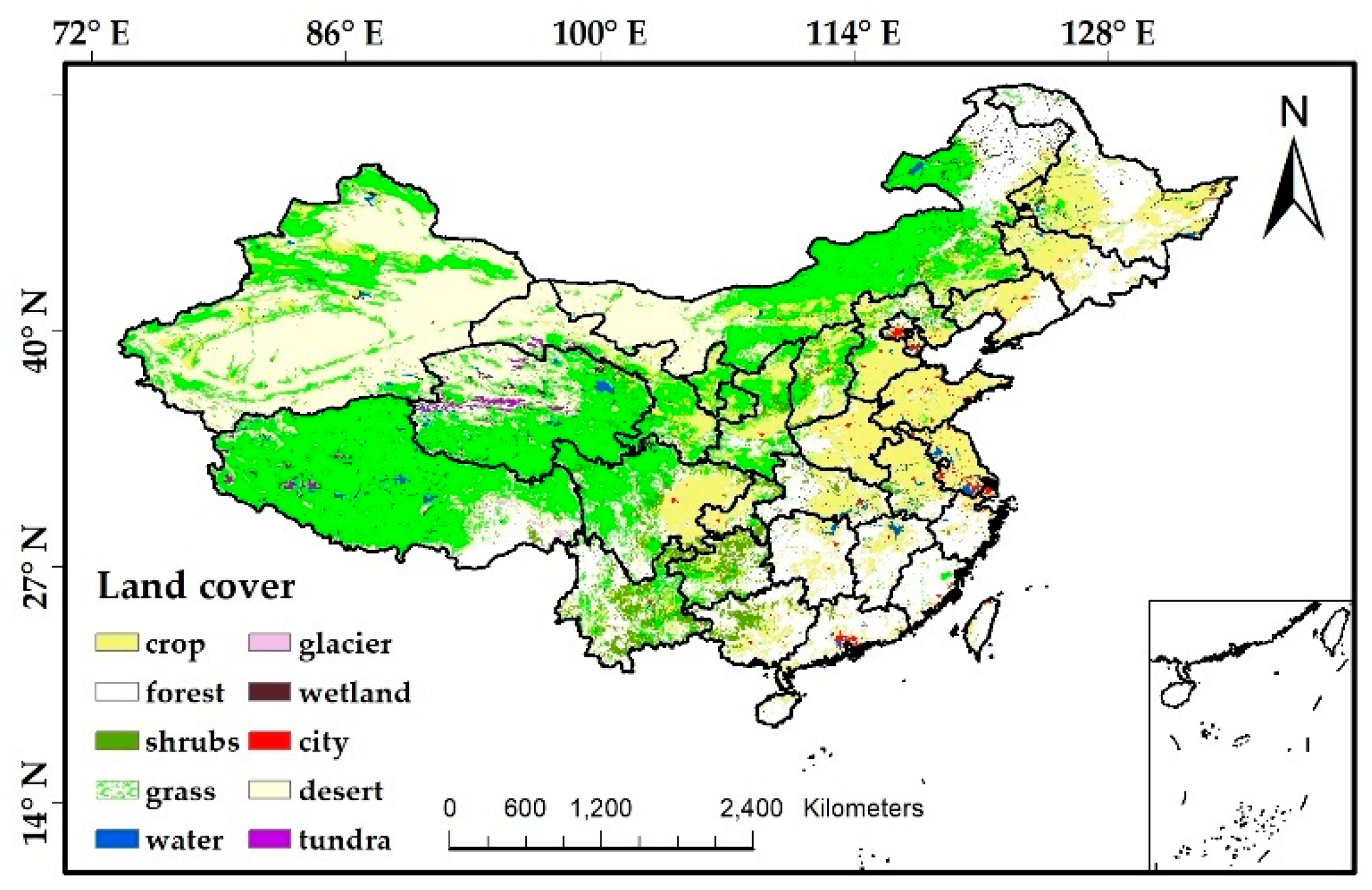
The study area is located throughout China (Figure 1). There are many types of land cover in China, ranging from 73°40′~135°2′E, 3°52′~53°33′N. The types of coverage are mainly grassland, cultivated land and woodland, but there are many other types of land use. The difference between China’s eastern and western regions is significant. The cultivated land and forest land are concentrated in the east, while the main land cover types in the western region are grassland and desert. The remote sensing features of different land types are very complex and have great differences in temporal and spatial distribution. Therefore, it is necessary to select a suitable quantitative remote sensing parameter rich in a large amount of land information for use in the land cover deep learning classification model.
2.2. Data
2.2.1. Land Cover Classification Sample
The training set, validation set and test set used in this study were derived from the 1 km CNLUCC dataset of the Institute of Geographical Sciences and Natural Resources Research, Chinese Academy of Sciences [52]. These data were resampled to a resolution of 0.05° by the method of majority resampling [53]. The dataset has been in existence every five years since 1980, and there is a lack of 1985 classification data. Due to the accuracy of the CNLUCC dataset and the mixed pixel problems caused by majority resampling, to ensure the reliability and credibility of the sample, we conducted a sample screening. When eight pixels around a pixel were the same, the cell in the center of the selection was considered to be a more reliable sample.
In this study, the 7-year 0.05° land cover classification data of 1980, 1990, 1995, 2000, 2005, 2010 and 2015 were filtered through reliability, and the 7-year samples were integrated and randomly disordered. From each category, 10% of the data were randomly extracted as a test set. The remaining samples were sample-tuned by a stratified SMOTE algorithm to obtain a training set. The sample distribution is shown in Table 1.
2.2.2. Land Cover Percentage Grading Sample
Since the CNLUCC 0.05° land cover classification data are obtained by the method of mode resampling, each pixel class is the category with the largest proportion of the 5 × 5 windows of the original 1 km land cover classification data. In addition to this, the cell also contains information about other categories in the original 5 × 5 window [54]. The land type of each pixel is represented by the category with the largest proportion of all pixels in the same area of the corresponding position in the original 1 km land use classification data in the pixel. Therefore, each pixel also contains the proportion information of other categories. Through this principle, the percentage data of other categories in the original 5 × 5 window are also obtained, and then, the data is discretized.
The specific method is that for a certain 0.05° land cover classification sample cell, the proportion of each category in the cell is divided into 6 levels by intervals of 20%. 0% is separated as an independent level. According to this method, we convert the obtained land cover percentage data into land cover percentage grading data. Based on this, a sample of land cover percentages was obtained.
2.2.3. Quantitative Remote Sensing Products
The data used in this study are mainly a variety of time series quantitative remote sensing products, including LAI, FAPAR, ET, GPP, and Albedo [21]. The leaf area index is defined as the multiple of the total leaf area of the plant and the unit land area, which is a characteristic parameter describing the vegetation canopy geometry. The fraction of absorbed photosynthetically active radiation is the ratio of the photosynthetically active radiation absorbed by plants to the incident solar radiation. The evapotranspiration index refers to the sum of the soil evaporation and plant transpiration. The surface albedo is defined as the ratio of the reflected reflectance to the incident degree of the target feature. The total primary productivity refers to the total amount of organic carbon fixed by the photosynthesis of green plants per unit time and unit area.
2.2.4. Supplementary Data
The temperature data [55] and precipitation data [56] of MERRA2 were also selected. The produce is reanalysis data obtained by the assimilation of site data and remote sensing data with a resolution of 0.625° × 0.5° [57], which is resampled to 0.05°.
The night light dataset of DMSP-OLS [58,59], which is based on the nighttime light signals detected by remote sensing satellites, is from the Defense Meteorological Satellite Program (DMSP). The nighttime lighting data comes from the DMSP/OLS night lighting products available in its visible and near-infrared sensors (DMSP/OLS). It is used to extract city categories with very good results [60]. Its spatial resolution is 30 arc second, which was resampled to 0.05°.
For classification, elevation, latitude and longitude information are also necessary, and different land cover types are related to the elevation, latitude and longitude [61]. In this study, the DEM data of ASTER GDEM [62] was obtained, which was also resampled to 0.05°, and the latitude and longitude information of the study area was extracted and input into the classification model. All data used in this study is shown in Table 2.
3. Methodology
3.1. Long Short-Term Memory Networks
Time series data are data collected at different points in time. These data reflect the state or extent of changes of a certain factor, phenomenon, and so on over time. LSTM are a kind of neural network used for processing sequence data. Typically, a neural network contains an input layer, one or several hidden layers and an output layer [63]. The output is controlled by the activation function, and the layers are connected by weights. The activation function is determined in advance. The underlying neural network only establishes a weighted connection between the layers, and the biggest difference of the LSTM is that the right connection is also established between neurons in the layer. A typical LSTM schematic is shown in Figure 2.
The sigmoid activation function [64] is represented by δ in Figure 2, and the calculation expressions of the three new gates, the hidden layer output and the state update Ct are as follows:
It can be seen that the inputs of these three doors are and , and each door has its own weight and skew. These parameters are tuned as the training process continues and play a role in the calculation of state updates and hidden layer output values.
3.2. Time Series Classification Based on the Bi-LSTM
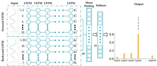
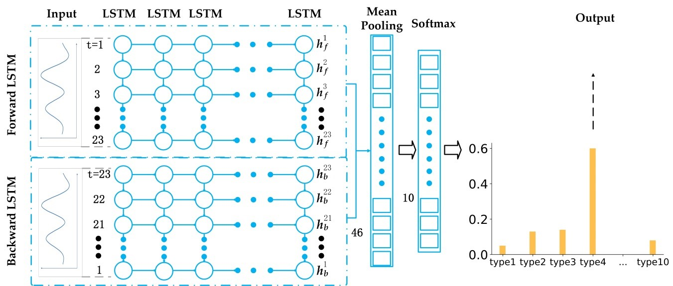
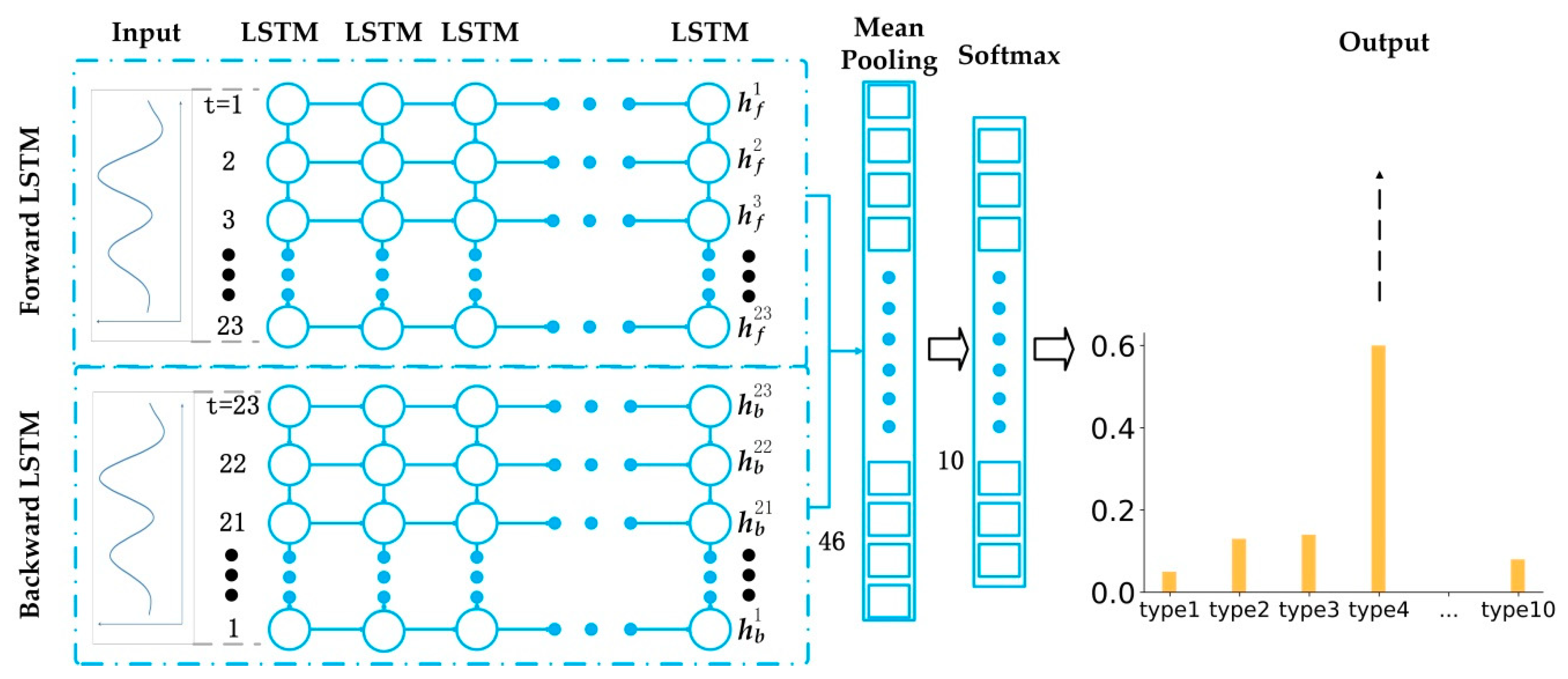
A multi-layer LSTM in two opposite directions [65] is used in this study to classify multiple categories of land cover through spatio-temporal data processing and multi-label land cover. The LSTM-based land cover classification model is shown in Figure 3. In Figure 3, the classification models are expanded in chronological order. The output layer originally existing in the LSTM network is removed. The output (, , …, , ) in the hidden layer is input into an averaged pooling layer to obtain a vector h without time information [66]. So far, an LSTM network was established with the output layer removed and added to the average pooling layer, called a Forward LSTM. At the same time, we also use a reverse version of the LSTM called the Backward LSTM. The two structures are basically the same, except that the Backward LSTM network requires the input data to be input in reverse order of the time series, and the output of this layer is represented by . Forward LSTM speculates the information based on the previous information, and Backward LSTM can push back the previous information by the following information. Bi-LSTM is a combination of Forward LSTM and Backward LSTM. This two-way information extraction is helpful for classification. Existing experiments have shown that the classification effect of Bi-LSTM is better than that of LSTM classification [67].
The land cover classification model takes the time series of multivariate quantitative remote sensing products as the input, and its output is the model’s estimate of the category label. It should be noted that the output of the ordinary RNN network or the LSTM network is a sequence of the same length as the input sequence, which is obviously inconsistent with the problem of the research. To this end, changes need to be made based on the LSTM model to adapt the output to the land cover classification problem.
To perform the task of classification, we construct a deep architecture with multiple layers of LSTMs stacked together, which will allow the extraction of advanced nonlinear time features in remote sensing time series. The proposed architecture is similar to the CNN network that combines several convolutional layers. Since the LSTM itself does not perform the task of class prediction, a softmax layer is added at the top of the LSTM network to perform multi-category predictions follow previous studies [68]. The category corresponding to the largest value in the softmax neuron is the final result of the prediction.
3.3. Time Series Percentage Grading Classification Extraction Model Based on the Bi-LSTM
After obtaining the long time series land cover classification product set, this study studies the percentage of long time series land cover category extraction. The land cover percentage grading model takes the multivariate quantitative remote sensing product time series and land cover classification data as input, and its output is an estimate of the model’s percentage proportion of the category. The structure of the model is basically the same as that of the LSTM-based land cover classification model. The difference is that the land cover data added in the input is used as a new feature, and the output of the model is changed to the estimate of the percentage level of the category. Since we need to obtain the proportions of different categories in each pixel, a percentage level extraction model for each category needs to be established to achieve the percentage ratio study of all categories. The specific approach is to extract the spatial distributions of all levels of the category for a certain category. The specific form of the performance is shown in Figure 4.
The different levels of pixels of the category are then extracted as samples as model inputs. Since the values of the percentages are discretized, the fitting work can be simplified into a classification task. When the model is trained, this study uses the level of the category as a label and uses land cover and quantitative remote sensing products as features. After the training, we predict the level of the category of the pixel by inputting quantitative remote sensing products and land cover. That is to say, the work of fitting a continuous percentage value of a category can be converted into a classification task of 6 levels of discrete values for the percentage of the category. Therefore, the land cover percentage grading model can be directly based on the framework of the land cover classification model, with the land cover percentage grading data and quantitative remote sensing products as inputs. Then, the land cover percentage grading model is constructed and trained. For the 10 categories, a total of 10 land cover percentage grading models need to be established.
3.4. Stratified SMOTE Algorithm
The different magnitudes of training samples have always been an unavoidable problem affecting the accuracy of deep learning models. To solve the imbalance of land cover samples, the traditional approach is to increase the number of small samples by upsampling and force the order of magnitude of the small samples to the same order of magnitude as the large samples. The common method is the SMOTE algorithm. In a nutshell, a new sample is generated for a few classes by means of “interpolation” [51]. The algorithm idea can be summarized in that for each sample x of a few classes, the distance from all samples in the minority sample set is calculated by the Euclidean distance standard, and the k-nearest neighbor is obtained. For each minority class sample x, several samples are randomly selected from their k nearest neighbors. Assuming that the nearest neighbor is , for each , a new sample is constructed according to Formula (6) using the original sample.
However, for the category samples of land cover classification, the sample sizes of different categories are very different. For example, a sample of the cultivated land category can reach the order of 300,000, while the sample size of the urban category is only 6000. When using the SMOTE algorithm, the city category sample will be increased from 6000 to 300,000. Among the results, the city’s 294,000 samples were obtained by SMOTE. It is very likely that the original characteristics of the city category will be lost, resulting in inaccuracies in the classification results [69].
To improve the inaccuracy of the classification caused by the excessive sample increase from the SMOTE algorithm, we used a sampling method called the stratified SMOTE algorithm to calibrate the sample [70]. The sample set obtained through the method and the sample set obtained through the traditional SMOTE algorithm are input into the model for training, and the results of the prediction are compared. The stratified SMOTE algorithm yields better results than does the traditional SMOTE algorithm. The number of small sample sizes can be increased within a reasonable range. This result will be discussed later.
The specific operation of the stratified SMOTE algorithm is to first count the number of samples in each category. Then, according to the order of magnitude of the samples, they are divided into three layers. The first layer is farmland, grassland, woodland and bare land. The second layer is shrubs. The third layer is wetland, water bodies, tundra, city and ice and snow. Then, the SMOTE algorithm is used in each of the three layers, and the sample set for the model training is obtained.
3.5. Evaluation
This study used the confusion matrix and the overall accuracy of the test set to evaluate the accuracy of the model and the classification results. The confusion matrix can calculate the accuracy of the classification of each category and evaluate the accuracies of different models relative to the overall accuracy. Then, this study also used the F1-score [71] as an indicator of the ability to classify of the model. This study also takes the user accuracy and charting accuracy of the classification model into account:
Here, is a single category of the F1-score, is the cartographic accuracy of the classification confusion matrix, and is the user precision of the classification confusion matrix. The F1-score used in this study is the average F1-score obtained by simply averaging the F1-scores of all categories.
Finally, the accuracy standard deviation is used as the evaluation index of the stability and applicability of the model in different years. One of the concerns of the long time series land cover classification model is ensuring that the model maintains a high and similarly stable classification accuracy for different years of classification results, and the accuracy standard deviation can provide this information.
4. Results
4.1. Model Accuracy and Importance Evaluation of Quantitative Remote Sensing Products
Random forests can assess the importance of different variables in the classification process through the Gini index [72,73]. From Figure 5 we can see the estimated importance of the variables of the data. Each histogram corresponds to a quantitative remote sensing parameter. The most important of these is GPP, ET ranks second, and NDVI ranks third. From this, we can find that quantitative remote sensing parameters are more important for classification than NDVI statistical indicators. It shows that quantitative remote sensing parameters play an important role in land cover classification.
To prove the performance and accuracy of the Bi-LSTM, this study also carried out a comparison of five types of machine learning models, Random Forest, SVM, CNN, LSTM and Bi-LSTM, for land cover classification studies. The difference between the Bi-LSTM and the LSTM is that the Bi-LSTM adds a layer of a neural network with reverse input data to extract more time information [74]. The CNN is a common convolutional neural network that is good at dealing with images, especially large image-related machine learning problems, and is often used in the spatial and spectral fields [75]. The way CNN works is to extract 2D spatial features. We used six quantitative remote sensing parameters, and the time dimension of each quantitative remote sensing parameter was 23 (equivalent to one data per half month). We take the six quantitative remote sensing parameters of each sample as the X-axis and the Y-axis as the time dimension to form a 6 × 23 2-dimensional input, then use the CNN model to convolve on this array, extract the features, and it carries out training and classification task. Then CNN usually extracts features layer-by-layer from multiple convolutional layers and pooling layers and finally completes classification through several fully connected layers. In this comparative experiment, for the three neural networks, a four-layer network structure is set up, and the number of neurons remains the same. When the accuracy of the training model is guaranteed to be stable, the five models all use the same test set to verify the accuracy of the model. The training process and final accuracy results of the model are shown in Table 3. In the case of using only the GPP as the input, the accuracies of the five neural network models reached a stable state, at 78.30%, 63.73%, 56.40%, 79.13%, and 81.86%, respectively, and the Bi-LSTM model had the highest accuracy.
Therefore, the Bi-LSTM is chosen as the classification model for long time series land cover classification task. At the same time, based on this, this study gradually increases the data in quantitative remote sensing products. For each additional quantitative remote sensing product, the accuracy of the classification model has been improved to a certain extent, finally achieving a classification accuracy of 88.04%, and its mean F1-score [76] value also reached 0.878. At the same time, the importance of the NDVI and quantitative remote sensing products is also evaluated. When the NDVI is removed and only the quantitative remote sensing product is used as the model input, the accuracy of the model is only reduced by 0.65%, indicating that the quantitative remote sensing product plays a leading role in this land cover classification model. Quantitative remote sensing products can be used as a new reliable factor for land cover classification research.
4.2. Long Time Series Classification Model Results
After inputting the dataset obtained from the layered SMOTE algorithm into the Bi-LSTM model, the model achieves an optimal state through multiple iterations. Therefore, the long time series land cover classification model is obtained. Generally speaking, for a deep learning model, the training accuracy of the model will continue to rise as iterations increase. When the model is trained to a certain extent, the model may have an over-fitting [77]. At this point, the generalization of the model will be reduced. The model works well on the training set, but it works poorly on the test set. So it is necessary to input the validation set to observe the test accuracy of the model [78]. In the learning curve, if the training accuracy and the validation accuracy are far apart, the variance of the model is large (in general, the training accuracy is higher than the validation accuracy), and the model is over-fitting. Ideally, the two precision curves of the training set and the validation set are close together. Once the classification accuracy of the validation set is saturated, the model is already in an optimal state. In the process of model training, the training precision curve, validation accuracy curve and loss function curve of the model are also depicted, as shown in Figure 6.
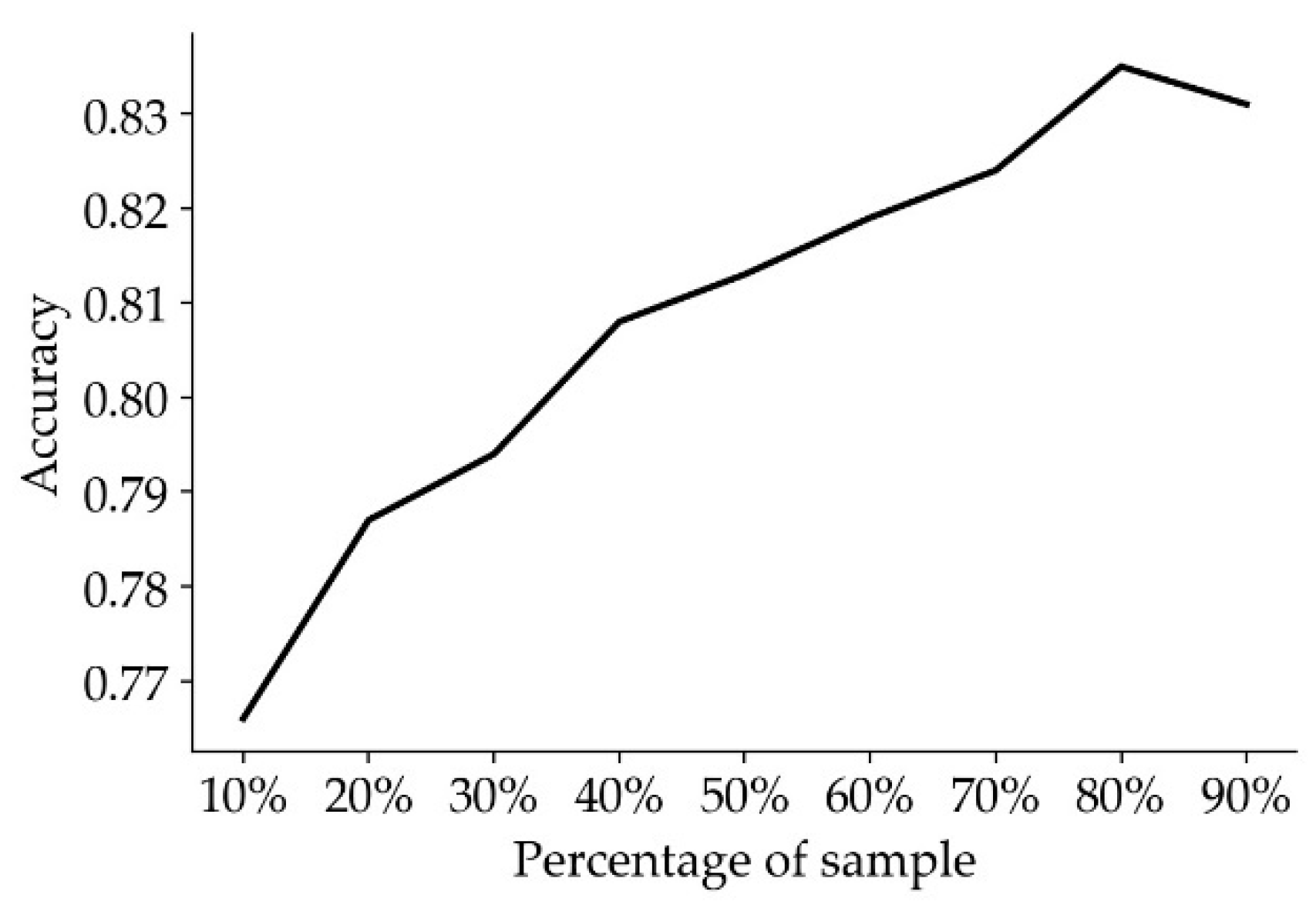
At the same time, the choice of the sample size of the training sample also affects the accuracy of the model. If the sample size is too small, the features of samples are not representative. In addition, if the sample size is too large, it will lead to an increase in the training time. To save training time and ensure training efficiency and training accuracy, we conducted experiments on the influence of different sample sizes on the accuracy of the model. Finally, we found that when we select 80% of the sample size as the training sample (Figure 7), the training effect of the model can achieve the best results.
The final test accuracy of the model is 84.2%. After inputting the test set into the model, the confusion matrix of the test set classification result is drawn. As shown in Table 4, the accuracy of each category has reached more than 80%, and the accuracies of the wetland, water, ice, snow, city, and tundra categories have reached more than 90%.
Since the goal is to obtain a long time series of land cover classification results, there is also a high requirement for the generalization ability of the model over time. Therefore, 10% of the samples from the CNLUCC classification data from 1980, 1990, 1995, 2000, 2005, 2010 and 2015 is extracted for test of the accuracy of the model and the accuracy of each category for the seven years. Furthermore, the standard deviation of the accuracy of each category during these seven years is determined. The errors for each category do not exceed 6%, and the error of the overall accuracy is maintained at 0.8%.
To further analyze the stability of the classification accuracy of the model, the maximum and minimum values and median of each category is also counted for different years and draws a box diagram (Figure 8). From this we can find that the accuracy of each category is kept at least 80%. The accuracy dispersion of a single category is relatively small. The accuracy of a single category is relatively small in time, and only three categories of forests, shrubs, and cities have outliers. However, the accuracy of these three outliers is greater than 80%, which is within an acceptable range. It is proven that the model also has good generalization for time series.
4.3. Land Cover Percentage Grading Model Results
After obtaining the land cover classification data for 2010, it is used as a common input along with the quantitative remote sensing products in 2010. The optimal state is achieved through multiple iterations of the model. Therefore, the land cover percentage grading model of 10 categories in 2010 was obtained. The training method and training process of the model are roughly the same as those of the land cover classification model.
After the test set are input into the trained model, the classification accuracies of the different levels of each category are obtained. According to the statistics, the results of the land cover percentage grading model training are relatively good. As shown in Table 5, the overall classification accuracy reached more than 85%, and the accuracies of 8 categories reached more than 90%.
5. Discussion
5.1. Use of Quantitative Remote Sensing Products
This study used a variety of quantitative remote sensing products, rather than only vegetation indices. The main reason behind this decision was that quantitative remote sensing products could reflect multiple ecological and physical characteristics of the surface at more levels [21,78]. The classification of the surface can be distinguished by more refined surface features. Among the features, LAI is a characteristic parameter describing the vegetation canopy geometry, which can reflect the growth and development of vegetation. FAPAR characterizes the intensity of photosynthesis in the vegetation. ET is an important process of water movement in a soil-plant-atmosphere continuous system. Its strength is closely related to the underlying surface conditions and plants. Albedo is an important parameter of the numerical climate model and the surface energy balance equation. GPP refers to the total amount of organic carbon fixed by the photosynthesis of green plants per unit time and unit area.
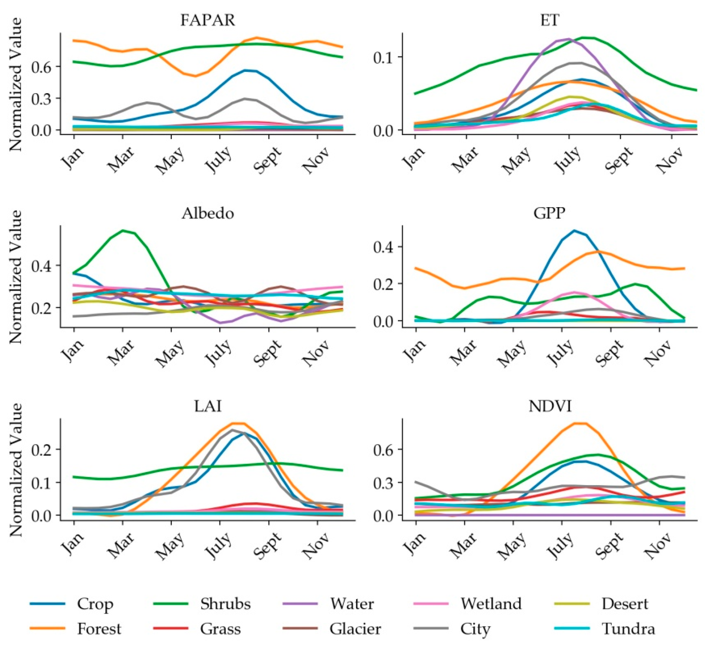
Vegetation first showed an increase and then a decrease in the NDVI year time series curve due to the growth cycle characteristics of budding-flowering-deciduous [79]. This feature contributes to the distinction between vegetation and non-vegetation. Because of human activities, cultivated land mostly undergoes two or three workings per year. Crops exhibit more than two peaks or three peaks on the NDVI year time series curve [80], and this curve has good characteristics for the distinction between crops and other vegetation in North China, South China and Sichuan. The albedo reflects the ability of the surface to absorb solar radiation. In general, the albedo of ice and snow is higher than those of other categories [81], followed by bare soil covered by waste soil and gravel. The albedo of a city is generally higher than that of vegetation or water. The albedo has a very good effect in distinguishing between cities and water bodies [82]. Grassland, woodland and shrubs also have certain differences in leaf area. The LAI also has a very good advantage in distinguishing between different vegetation groups [83]. The GPP, ET and FAPAR have explained the differences in the inter-annual variations of different types of land types from biological and thermal aspects. As shown in Figure 9, the performance of different land types in quantitative remote sensing parameters is different. The different performances of quantitative remote sensing products of different land types in one year is the theoretical basis for the long time series land cover classification.
Through the evaluation of the feature importance of random forests, feature importance of each category was extracted in the classification process, as shown in Figure 10. The first is cultivated land. ET and NDVI are more important for the crop category, mainly due to the cyclical NDVI characteristics of crops and the strong correlation between crops and ET [84]. Forest is mainly affected by NDVI and LAI. Mainly because of the high vegetation coverage of forest land. The vegetation coverage of grassland is similar to the coverage of forest land, shrubs and crops, but in GPP it may be lower than these three categories, so the importance of GPP will be higher. Because of its high albedo, the feature importance of glacier is higher in albedo. Cities are more affected by ET and albedo. GPP and NDVI are of high feature importance to the desert due to their extremely low GPP values and lower NDVI values. These results confirm to some extent the conclusion that quantitative remote sensing parameters are helpful for land cover classification.
By extracting the annual characteristic curves of six quantitative remote sensing products as the input of the model, the model does not just obtain the characteristic parameter information of various surfaces but can also obtain the time change information. The time performance of different surface parameters in the same feature parameter is also different. This time information is also provided to the classification model, which has a very positive effect on the classification of different categories.
5.2. Sample Equalization Method
To solve the classification accuracy problem caused by the sample size difference between categories, we choose SMOTE method which could solve the gap problem of the sample size. However, this method cannot be directly applied into our study because the sample size difference between the categories with the largest sample number and the minimum sample size is too large, which causes most samples of the category to be interpolated and causes samples of small sample categories to lose their original basic characteristics [85].
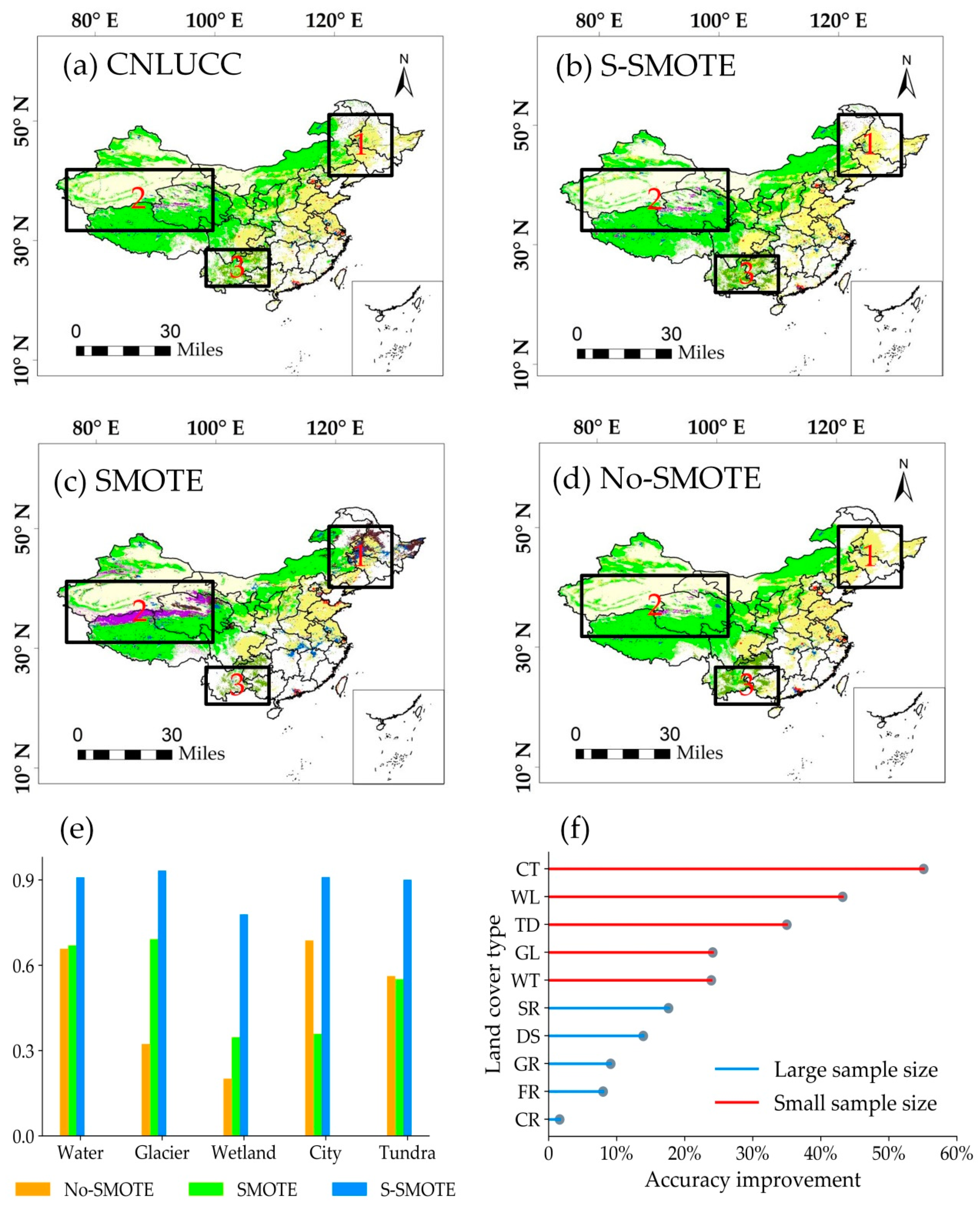
Although the sample set obtained from the SMOTE algorithm can yield a better training accuracy and test accuracy, it is found that the China 2010 classified products obtained by this method are quite different from the 2010 CNLUCC classified products in China. The main differences are distributed in the areas enclosed by the three rectangular boxes shown in Figure 11.
- The region 1 rectangular frame indicates the northeastern region of China. Among the CNLUCC land cover classification products, the main land cover types in the area are cultivated land and forest land, and a small amount of water is covered in the middle. This result is consistent with the actual land cover type in the area. However, in the results obtained from the SMOTE algorithm, it can be found that a large number of water bodies have appeared in Northeast China.
- The region 2 rectangular frame indicates the western part of China. Among the CNLUCC land cover classification products, the main land cover types in the area are grassland and bare land, and a small amount of tundra covers the middle. This result is consistent with the actual land cover type in the area. However, in the results obtained from the SMOTE algorithm, it can be found that a large number of tundra distributions occur in western China.
- The region 3 rectangular frame indicates the southwestern region of China. Among the CNLUCC land cover classification products, the main land cover types in the area are woodland and shrubs, in which shrubs and woodlands are intersecting. This result is consistent with the actual land cover type in the area. However, in the results obtained from the SMOTE algorithm, it can be found that a large number of dense shrubs are distributed in southwestern China. The results of the above three regions obtained through the SMOTE algorithm are obviously not consistent with the actual land cover.
To correct this problem, this study improves the SMOTE algorithm and uses the stratified SMOTE algorithm. After inputting the dataset obtained from the algorithm into the model and after several iterations, it finds that the training accuracy and test accuracy of the land cover classification model can also achieve good results. To prove that the stratified SMOTE algorithm has a positive effect on the actual classification results, the dataset obtained from the algorithm to acquire the 2010 land cover type products was this study used. The results were compared with the 2010 products obtained from CNLUCC products and the 2010 products obtained from the SMOTE algorithm, as shown in Figure 11. The misclassification of areas within the corresponding three rectangular boxes is very well solved. In addition, the results of the two SMOTE algorithms are referenced to CNLUCC data, and the number of correctly classified cells in the 10 categories of the two algorithms is counted. The results after statistics are shown in Table 6. For each category, the stratified SMOTE algorithm improves the accuracy of the classification, and the method is simple and effective. The accuracies of the six small sample categories of shrubs, water bodies, ice and snow, wetland cities and tundra are much higher.
5.3. Sample Selection for Accuracy Assessment Methods
The sample in this study was collected from the CNLUCC China Land Cover Classification Dataset of the Institute of Geographical Sciences and Natural Resources Research, Chinese Academy of Sciences. The training set, validation set and test set were obtained from this dataset. To ensure the reliability of the sample, when the eight pixels around the central pixel are the same, the central pixel of the selected center is considered to be a highly reliable sample. All the samples selected for accuracy assessment are obtained by this method. For land cover classification studies, the best test set are generally field data, and the results are closest to the actual land categories.
However, it is not realistic to obtain annual actual test set for long time series land cover classification research, which requires a large amount manpower and time, and there are currently no relevant test set. Most of the test set are collected during a given year and does not reflect changes in land cover. Furthermore, each cell of the 0.05° classification data covers a larger area. Due to the scale effect, the field data does not reflect the actual category of 0.05° pixels. The sliding window is used to ensure that the sample is consistent with the surrounding pixel categories. The sliding window can be filtered to ensure the purity of the sample under limited conditions, thus ensuring the accuracy of the sample. Under the premise of ensuring the accuracy of the sample, the results obtained using the field sample for classification studies are also acceptable [76].
5.4. Model Stability Analysis
This study performed a statistical analysis of the accuracy of different years for each category in Section 4.2. In addition, we found that the accuracy is good in each year. Moreover, the annual accuracy has good stability. The results show that the accuracy of the different years for each category is roughly the same. The standard deviation of interannual precision is no more than 6%. However, the accuracy of the wetland has a higher dispersion than the other categories, with a difference of 13.3% between the maximum and the minimum. Although the accuracy is still high (85.4% for the year of the lowest precision), it has awful stability of the different years for wetland.
We hold it is the following two reasons that cause the problem. Firstly, there are many types of wetlands such as coastal wetland, inland wetland and artificial wetland [86]. Wetlands occupy an intermediate position between truly terrestrial and aquatic ecosystems and therefore encompass a diverse array of habitats. This array of habitats is difficult to define [87]. In addition, there are many different types of organisms in the wetlands. Therefore, the quantitative remote sensing characteristics of wetlands are complex and easily confused with water bodies and other vegetation types. At the same time, the sample size of the wetland is too small, so the model is easy to misclassify the wetland into other categories. Secondly, in terms of methods, we use time series quantitative remote sensing features to classify land cover. However, the similarity in time series between wetlands and other categories can cause certain difficulties for our classification task. We will improve in the follow-up work in this part of the study.
6. Conclusions
A long time series land cover classification deep learning model based on the Bi-LSTM is proposed. This model uses CNLUCC China land cover classification data to form a set of long time series land cover classification samples. Then, the corresponding relationship between the land cover type and the sequence quantitative remote sensing products is established. Afterward, a self-classification model of 0.05° long time series land cover depth learning in China was trained, and the accuracy of the model was evaluated.
The LSTM model has advantages over other models in processing time series data, which preserves the temporal information of the data for time series classification. A set of data was used to train and compare the accuracies of three deep learning models, the CNN, LSTM and Bi-LSTM. The Bi-LSTM model achieves higher accuracy with consistent parameters. Therefore, the Bi-LSTM model was chosen as the basic model for the long time series land cover model.
In this study, the long time series land cover classification sample set is randomly disrupted and input into the Bi-LSTM model to carry out model training. In the process of model training, the training process of the model is monitored through visual operation. Since the deep learning model may begin over-fitting after the number of training iterations reaches a certain level, it is necessary to monitor the process of the model. The training is ended after the model test accuracy has stabilized and before the test accuracy has decreased. Finally, a long time series land cover classification model was obtained with an overall accuracy of 84.2%.
The CNLUCC China land cover classification data in 1980, 1990, 1995, 2000, 2005, 2010 and 2015 is used as a reference to evaluate the accuracy of the land cover classification data obtained in the same years. There are 10 categories with accuracies of over 82%, and 5 of them have accuracies of over 90%. While ensuring the accuracy, we evaluate the classification accuracies of different years for the same category. The results show that the accuracies of different years for the same category are about the same, and the deviation is not large. The errors of 10 categories are not more than 6%, and the accuracy error does not exceed 0.8%. Due to the large amount of mixed category information contained in the 5 km classification pixels, we also extract the information by grading, and the overall classification accuracy of each category reached more than 85%. There are 8 categories with accuracies of over 90%, which proves the feasibility and reliability of the Bi-LSTM model for time series land cover classification.
Author Contributions
H.W. and X.Z. conceived of and designed the experiments. H.W. processed and analyzed the data. All authors contributed to the ideas, writing, and discussion.
Funding
This study was supported by the National Key Research and Development Program of China (No. 2016YFB0501404).
Acknowledgments
The authors thank Qian Wang, Jia Chen, Rongyun Tang and Yifeng Peng for helpful comments that improved this manuscript.
Conflicts of Interest
The authors declare no conflict of interest.
References
- Feddema, J.J.; Oleson, K.W.; Bonan, G.B.; Mearns, L.O.; Buja, L.E.; Meehl, G.A.; Washington, W.M. The Importance of Land-Cover Change in Simulating Future Climates. Science 2005, 310, 1674–1678. [Google Scholar] [CrossRef] [PubMed] [Green Version]
- Wulder, M.A.; White, J.C.; Goward, S.N.; Masek, J.G.; Irons, J.R.; Herold, M.; Cohen, W.B.; Loveland, T.R.; Woodcock, C. Landsat continuity: Issues and opportunities for land cover monitoring. Remote Sens. Environ. 2008, 112, 955–969. [Google Scholar] [CrossRef]
- Bathiany, S.; Claussen, M.; Brovkin, V.; Raddatz, T.; Gayler, V. Combined biogeophysical and biogeochemical effects of large-scale forest cover changes in the MPI earth system model. Biogeosciences 2010, 7, 1383–1399. [Google Scholar] [CrossRef] [Green Version]
- Fu, P.; Weng, Q. A time series analysis of urbanization induced land use and land cover change and its impact on land surface temperature with Landsat imagery. Remote Sens. Environ. 2016, 175, 205–214. [Google Scholar] [CrossRef]
- Lambin, E.F.; Geist, H.J.; Lepers, E. Dynamics of land-use and land-cover change in tropical regions. Annu. Rev. Environ. 2003, 28, 205–241. [Google Scholar] [CrossRef]
- Liu, D.; Cai, S. A spatial-temporal modeling approach to reconstructing land-cover change trajectories from multi-temporal satellite imagery. Ann. Assoc. Am. Geogr. 2012, 102, 1329–1347. [Google Scholar] [CrossRef]
- Rogan, J.; Chen, D. Remote sensing technology for mapping and monitoring land-cover and land-use change. Prog. Plan. 2004, 61, 301–325. [Google Scholar] [CrossRef]
- Pal, S.; Ziaul, S. Detection of land use and land cover change and land surface temperature in English Bazar urban centre. Egypt. J. Remote Sens. 2017, 20, 125–145. [Google Scholar] [CrossRef] [Green Version]
- Hussain, M.; Chen, D.; Cheng, A.; Wei, H.; Stanley, D. Change detection from remotely sensed images: From pixel-based to object-based approaches. ISPRS J. Photogramm. 2013, 80, 91–106. [Google Scholar] [CrossRef]
- Hegazy, I.R.; Kaloop, M.R. Monitoring urban growth and land use change detection with GIS and remote sensing techniques in Daqahlia governorate Egypt. Int. J. Sustain. Built Environ. 2015, 4, 117–124. [Google Scholar] [CrossRef] [Green Version]
- Loveland, T.R.; Belward, A. The IGBP-DIS global 1km land cover data set, DISCover: First results. Int. J. Remote Sens. 1997, 18, 3289–3295. [Google Scholar] [CrossRef]
- Vogelmann, J.E.; Howard, S.M.; Yang, L.; Larson, C.R.; Wylie, B.K.; Van Driel, N. Completion of the 1990s National Land Cover Data Set for the Conterminous United States from Landsat Thematic Mapper Data and Ancillary Data Sources. Am. Soc. Photogram. Remote Sens. 2010, 67, 650–655. [Google Scholar]
- Friedl, M.A.; Sulla-Menashe, D.; Tan, B.; Schneider, A.; Ramankutty, N.; Sibley, A.; Huang, X. MODIS Collection 5 global land cover: Algorithm refinements and characterization of new datasets. Remote Sens. Environ. 2010, 114, 168–182. [Google Scholar] [CrossRef]
- Pouliot, D.; Latifovic, R.; Zabcic, N.; Guindon, L.; Olthof, I. Development and assessment of a 250 m spatial resolution MODIS annual land cover time series (2000–2011) for the forest region of Canada derived from change-based updating. Remote Sens. Environ. 2014, 140, 731–743. [Google Scholar] [CrossRef]
- Gray, J.; Song, C. Consistent classification of image time series with automatic adaptive signature generalization. Remote Sens. Environ. 2013, 134, 333–341. [Google Scholar] [CrossRef]
- Song, C.; Woodcock, C.E.; Seto, K.C.; Lenney, M.P.; Macomber, S.A. Classification and change detection using Landsat TM data: When and how to correct atmospheric effects? Remote Sens. Environ. 2001, 75, 230–244. [Google Scholar] [CrossRef]
- Yu, W.; Zhou, W.; Qian, Y.; Yan, J. A new approach for land cover classification and change analysis: Integrating backdating and an object-based method. Remote Sens. Environ. 2016, 177, 37–47. [Google Scholar] [CrossRef]
- Melgani, F.; Bruzzone, L. Classification of hyperspectral remote sensing images with support vector machines. IEEE Trans. Geosci. Remote Sens. 2004, 42, 1778–1790. [Google Scholar] [CrossRef] [Green Version]
- Franklin, S.E.; Ahmed, O.S.; Wulder, M.A.; White, J.C.; Hermosilla, T.; Coops, N.C. Large area mapping of annual land cover dynamics using multitemporal change detection and classification of Landsat time series data. Can. J. Remote Sens. 2015, 41, 293–314. [Google Scholar] [CrossRef]
- Shao, Y.; Lunetta, R.S.; Wheeler, B.; Iiames, J.S.; Campbell, J.B. An evaluation of time-series smoothing algorithms for land-cover classifications using MODIS-NDVI multi-temporal data. Remote Sens. Environ. 2016, 174, 258–265. [Google Scholar] [CrossRef]
- Liang, S.; Zhao, X.; Liu, S.; Yuan, W.; Cheng, X.; Xiao, Z.; Zhang, X.; Liu, Q.; Cheng, J.; Tang, H. A long-term Global LAnd Surface Satellite (GLASS) data-set for environmental studies. Int. J. Digit. Earth 2013, 6, 5–33. [Google Scholar] [CrossRef]
- He, T.; Liang, S.; Song, D.X. Analysis of global land surface albedo climatology and spatial-temporal variation during 1981–2010 from multiple satellite products. J. Geophys. Res. Atmos. 2014, 119, 10281–10298. [Google Scholar] [CrossRef]
- Nishida, K.; Nemani, R.R.; Glassy, J.M.; Running, S.W. Development of an evapotranspiration index from Aqua/MODIS for monitoring surface moisture status. IEEE Trans. Geosci. Remote Sens. 2003, 41, 493–501. [Google Scholar] [CrossRef]
- Xiao, Z.; Liang, S.; Wang, J.; Xiang, Y.; Zhao, X.; Song, J. Long-time-series global land surface satellite leaf area index product derived from MODIS and AVHRR surface reflectance. IEEE Trans. Geosci. Remote Sens. 2016, 54, 5301–5318. [Google Scholar] [CrossRef]
- Zhang, X.; Liang, S.; Zhou, G.; Wu, H.; Zhao, X. Generating Global LAnd Surface Satellite incident shortwave radiation and photosynthetically active radiation products from multiple satellite data. Remote Sens. Environ. 2014, 152, 318–332. [Google Scholar] [CrossRef]
- Xiao, Z.; Liang, S.; Sun, R.; Wang, J.; Jiang, B. Estimating the fraction of absorbed photosynthetically active radiation from the MODIS data-based GLASS leaf area index product. Remote Sens. Environ. 2015, 171, 105–117. [Google Scholar] [CrossRef]
- Dhodhi, M.K.; Saghri, J.A.; Ahmad, I.; Ul-Mustafa, R. D-ISODATA: A distributed algorithm for unsupervised classification of remotely sensed data on network of workstations. J. Parallel Distrib. Comput. 1999, 59, 280–301. [Google Scholar] [CrossRef]
- Otukei, J.R.; Blaschke, T. Land cover change assessment using decision trees, support vector machines and maximum likelihood classification algorithms. Int. J. Appl. Earth Obs. Geoinf. 2010, 12, S27–S31. [Google Scholar] [CrossRef]
- Lv, Z.; Hu, Y.; Zhong, H.; Wu, J.; Li, B.; Zhao, H. Parallel k-means clustering of remote sensing images based on mapreduce. In International Conference on Web Information Systems and Mining; Springer: Berlin/Heidelberg, Germany, 2010; pp. 162–170. [Google Scholar]
- Gopal, S.; Woodcock, C.E.; Strahler, A.H. Fuzzy neural network classification of global land cover from a 1 AVHRR data set. Remote Sens. Environ. 1999, 67, 230–243. [Google Scholar] [CrossRef]
- Boles, S.H.; Xiao, X.; Liu, J.; Zhang, Q.; Munkhtuya, S.; Chen, S.; Ojima, D. Land cover characterization of Temperate East Asia using multi-temporal VEGETATION sensor data. Remote Sens. Environ. 2004, 90, 477–489. [Google Scholar] [CrossRef]
- Homer, C.; Huang, C.; Yang, L.; Wylie, B.; Coan, M. Development of a 2001 national land-cover database for the United States. J. Photogramm. Eng. Remote Sens. 2004, 70, 829–840. [Google Scholar] [CrossRef]
- Carrão, H.; Gonçalves, P.; Caetano, M. Contribution of multispectral and multitemporal information from MODIS images to land cover classification. Remote Sens. Environ. 2008, 112, 986–997. [Google Scholar] [CrossRef]
- Gómez, C.; White, J.C.; Wulder, M.A. Optical remotely sensed time series data for land cover classification: A review. ISPRS J. Photogramm. Remote Sens. 2016, 116, 55–72. [Google Scholar] [CrossRef] [Green Version]
- Qian, Y.; Zhou, W.; Yan, J.; Li, W.; Han, L. Comparing machine learning classifiers for object-based land cover classification using very high resolution imagery. Remote Sens. 2015, 7, 153–168. [Google Scholar] [CrossRef]
- Qiu, J.; Wu, Q.; Ding, G.; Xu, Y.; Feng, S. A survey of machine learning for big data processing. EURASIP J. Adv. Signal Process. 2016, 2016, 67. [Google Scholar] [CrossRef]
- Zhu, X.X.; Tuia, D.; Mou, L.; Xia, G.-S.; Zhang, L.; Xu, F.; Fraundorfer, F. Deep learning in remote sensing: A comprehensive review and list of resources. IEEE Geosci. Remote Sens. Mag. 2017, 5, 8–36. [Google Scholar] [CrossRef]
- Romero, A.; Gatta, C.; Camps-Valls, G. Unsupervised deep feature extraction for remote sensing image classification. IEEE Trans. Geosci. Remote Sens. 2015, 54, 1349–1362. [Google Scholar] [CrossRef]
- Chen, Y.; Lin, Z.; Zhao, X.; Wang, G.; Gu, Y. Deep learning-based classification of hyperspectral data. IEEE J. Sel. Top. Appl. Earth Obs. Remote Sens. 2014, 7, 2094–2107. [Google Scholar] [CrossRef]
- Hu, F.; Xia, G.-S.; Hu, J.; Zhang, L. Transferring deep convolutional neural networks for the scene classification of high-resolution remote sensing imagery. Remote Sens. 2015, 7, 14680–14707. [Google Scholar] [CrossRef]
- Zhang, L.; Zhang, L.; Du, B. Deep learning for remote sensing data: A technical tutorial on the state of the art. IEEE Geosci. Remote Sens. Mag. 2016, 4, 22–40. [Google Scholar] [CrossRef]
- Maggiori, E.; Tarabalka, Y.; Charpiat, G.; Alliez, P. Convolutional neural networks for large-scale remote-sensing image classification. IEEE Trans. Geosci. Remote Sens. 2017, 55, 645–657. [Google Scholar] [CrossRef]
- Yu, S.; Jia, S.; Xu, C. Convolutional neural networks for hyperspectral image classification. Neurocomputing 2017, 219, 88–98. [Google Scholar] [CrossRef]
- Hochreiter, S.; Schmidhuber, J. Long short-term memory. Neural Comput. 1997, 9, 1735–1780. [Google Scholar] [CrossRef] [PubMed]
- Ienco, D.; Gaetano, R.; Dupaquier, C.; Maurel, P. Land cover classification via multi-temporal spatial data by recurrent neural networks. IEEE Geosci. Remote Sens. Lett. 2017, 14, 1685–1689. [Google Scholar] [CrossRef]
- Mou, L.; Bruzzone, L.; Zhu, X.X. Learning spectral-spatial-temporal features via a recurrent convolutional neural network for change detection in multispectral imagery. IEEE Trans. Geosci. Remote Sens. 2019, 57, 924–935. [Google Scholar] [CrossRef]
- Lyu, H.; Lu, H.; Mou, L. Learning a transferable change rule from a recurrent neural network for land cover change detection. Remote Sens. 2016, 8, 506. [Google Scholar] [CrossRef]
- Rußwurm, M.; Körner, M. Multi-temporal land cover classification with long short-term memory neural networks. Int. Arch. Photogramm. Remote Sens. Spat. Inf. Sci. 2017, 42, 551. [Google Scholar] [CrossRef]
- Mellor, A.; Boukir, S.; Haywood, A.; Jones, S. Exploring issues of training data imbalance and mislabelling on random forest performance for large area land cover classification using the ensemble margin. ISPRS J. Photogramm. Remote Sens. 2015, 105, 155–168. [Google Scholar] [CrossRef]
- Estabrooks, A.; Jo, T.; Japkowicz, N. A multiple resampling method for learning from imbalanced data sets. Comput. Intell. 2004, 20, 18–36. [Google Scholar] [CrossRef]
- Chawla, N.V.; Bowyer, K.W.; Hall, L.O.; Kegelmeyer, W.P. SMOTE: Synthetic minority over-sampling technique. J. Artif. Intell. Res. 2002, 16, 321–357. [Google Scholar] [CrossRef]
- Xu, X.; Liu, J.; Zhang, S.; Li, R.; Yan, C.; Wu, S. China’s Multi-Period Land Use Land Cover Remote Sensing Monitoring Data Set (CNLUCC); Resource and Environment Data Cloud Platform: Beijing, China, 2018. [Google Scholar]
- Tao, X.; Liang, S.; Wang, D. Assessment of five global satellite products of fraction of absorbed photosynthetically active radiation: Intercomparison and direct validation against ground-based data. Remote Sens. Environ. 2015, 163, 270–285. [Google Scholar] [CrossRef]
- Sulla-Menashe, D.; Friedl, M.A. User Guide to Collection 6 MODIS Land Cover (MCD12Q1 and MCD12C1) Product; USGS: Reston, VA, USA, 2018.
- Lim, Y.-K.; Schubert, S.D.; Nowicki, S.M.; Lee, J.N.; Molod, A.M.; Cullather, R.I.; Zhao, B.; Velicogna, I. Atmospheric summer teleconnections and Greenland Ice Sheet surface mass variations: Insights from MERRA-2. Environ. Res. Lett. 2016, 11, 024002. [Google Scholar] [CrossRef]
- Reichle, R.H.; Liu, Q.; Koster, R.D.; Draper, C.S.; Mahanama, S.P.; Partyka, G.S. Land surface precipitation in MERRA-2. J. Clim. 2017, 30, 1643–1664. [Google Scholar] [CrossRef]
- Bosilovich, M.; Lucchesi, R.; Suarez, M. MERRA-2: File Specification; GMAO Office Note NO.9(Version 1.0); 2015. Available online: https://ntrs.nasa.gov/search.jsp?R=20150019760 (accessed on 1 June 2019).
- Elvidge, C.D.; Baugh, K.E.; Kihn, E.A.; Kroehl, H.W.; Davis, E.R. Mapping city lights with nighttime data from the DMSP Operational Linescan System. Photogramm. Eng. Remote Sens. 1997, 63, 727–734. [Google Scholar]
- Zhou, Y.; Smith, S.J.; Zhao, K.; Imhoff, M.; Thomson, A.; Bond-Lamberty, B.; Asrar, G.R.; Zhang, X.; He, C.; Elvidge, C.D. A global map of urban extent from nightlights. Environ. Res. Lett. 2015, 10, 054011. [Google Scholar] [CrossRef]
- Zhou, Y.; Smith, S.J.; Elvidge, C.D.; Zhao, K.; Thomson, A.; Imhoff, M. A cluster-based method to map urban area from DMSP/OLS nightlights. Remote Sens. Environ. 2014, 147, 173–185. [Google Scholar] [CrossRef]
- Fahsi, A.; Tsegaye, T.; Tadesse, W.; Coleman, T. Incorporation of digital elevation models with Landsat-TM data to improve land cover classification accuracy. For. Ecol. Manag. 2000, 128, 57–64. [Google Scholar] [CrossRef]
- Tachikawa, T.; Kaku, M.; Iwasaki, A.; Gesch, D.B.; Oimoen, M.J.; Zhang, Z.; Danielson, J.J.; Krieger, T.; Curtis, B.; Haase, J. ASTER Global Digital Elevation Model Version 2-Summary of Validation Results; NASA, 2011. Available online: https://pubs.er.usgs.gov/publication/70005960 (accessed on 1 June 2019).
- Da Silva, I.N.; Spatti, D.H.; Flauzino, R.A.; Liboni, L.H.B.; dos Reis Alves, S.F. Artificial Neural Networks; Springer International Publishing: Cham, Switzerland, 2017. [Google Scholar]
- Yin, X.; Goudriaan, J.; Lantinga, E.A.; Vos, J.; Spiertz, H.J. A flexible sigmoid function of determinate growth. Ann. Bot. 2003, 91, 361–371. [Google Scholar] [CrossRef] [PubMed]
- Mei, X.; Pan, E.; Ma, Y.; Dai, X.; Huang, J.; Fan, F.; Du, Q.; Zheng, H.; Ma, J. Spectral-Spatial Attention Networks for Hyperspectral Image Classification. Remote Sens. 2019, 11, 963. [Google Scholar] [CrossRef]
- Sun, Z.; Di, L.; Fang, H. Using long short-term memory recurrent neural network in land cover classification on Landsat and Cropland data layer time series. Int. J. Remote Sens. 2019, 40, 593–614. [Google Scholar] [CrossRef]
- Graves, A. Long Short-Term Memory. Supervised Sequence Labelling with Recurrent Neural Networks; Springer, 2012; pp. 37–45. Available online: https://0-link-springer-com.brum.beds.ac.uk/chapter/10.1007/978-3-642-24797-2_4 (accessed on 1 June 2019).
- Liu, P.; Qiu, X.; Huang, X. Recurrent neural network for text classification with multi-task learning. arXiv 2016, arXiv:1605.05101. [Google Scholar]
- Hu, Y.; Guo, D.; Fan, Z.; Dong, C.; Huang, Q.; Xie, S.; Liu, G.; Tan, J.; Li, B.; Xie, Q. An improved algorithm for imbalanced data and small sample size classification. J. Data Anal. Inf. Process. 2015, 3, 27. [Google Scholar] [CrossRef]
- Zhao, H.; Chen, X.; Nguyen, T.; Huang, J.Z.; Williams, G.; Chen, H. Stratified over-sampling bagging method for random forests on imbalanced data. In Proceedings of the 2016 Pacific-Asia Workshop on Intelligence and Security Informatics, Auckland, New Zealand, 19 April 2016; pp. 63–72. [Google Scholar]
- Goutte, C.; Gaussier, E. A probabilistic interpretation of precision, recall and F-score, with implication for evaluation. In Proceedings of the European Conference on Information Retrieval, Santiago de Compostela, Spain, 21–23 March 2005; pp. 345–359. [Google Scholar]
- Gislason, P.O.; Benediktsson, J.A.; Sveinsson, J. Random forests for land cover classification. Pattern Recognit. Lett. 2006, 27, 294–300. [Google Scholar] [CrossRef]
- Rodriguez-Galiano, V.F.; Ghimire, B.; Rogan, J.; Chica-Olmo, M.; Rigol-Sanchez, J.P.; Sensing, R. An assessment of the effectiveness of a random forest classifier for land-cover classification. ISPRS J. Photogramm. Remote Sens. 2012, 67, 93–104. [Google Scholar] [CrossRef]
- Graves, A.; Schmidhuber, J. Framewise phoneme classification with bidirectional LSTM and other neural network architectures. Neural Netw. 2005, 18, 602–610. [Google Scholar] [CrossRef] [PubMed]
- Dang, Y.; Zhang, J.; Zhao, Y.; Luo, F.; Ma, W.; Yu, F. Quality Evaluation of Land-Cover Classification Using Convolutional Neural Network. Int. Arch. Photogramm. Remote Sens. Spat. Inf. Sci. 2018, XLII-3, 257–262. [Google Scholar] [CrossRef]
- Zhong, L.; Hu, L.; Zhou, H. Deep learning-based multi-temporal crop classification. Remote Sens. Environ. 2019, 221, 430–443. [Google Scholar] [CrossRef]
- Hawkins, D.M. The problem of overfitting. J. Chem. Inf. Comput. Sci. 2004, 44, 1–12. [Google Scholar] [CrossRef] [PubMed]
- Yeom, S.; Giacomelli, I.; Fredrikson, M.; Jha, S. Privacy risk in machine learning: Analyzing the connection to overfitting. In Proceedings of the 2018 IEEE 31st Computer Security Foundations Symposium (CSF), Oxford, UK, 9–12 July 2018; pp. 268–282. [Google Scholar]
- Gandhi, G.M.; Parthiban, S.; Thummalu, N.; Christy, A. NDVI: Vegetation change detection using remote sensing and GIS—A case study of Vellore District. Procedia Comput. Sci. 2015, 57, 1199–1210. [Google Scholar] [CrossRef]
- Sakamoto, T.; Yokozawa, M.; Toritani, H.; Shibayama, M.; Ishitsuka, N.; Ohno, H. A crop phenology detection method using time-series MODIS data. Remote Sens. Environ. 2005, 96, 366–374. [Google Scholar] [CrossRef]
- Dozier, J.; Marks, D. Snow mapping and classification from Landsat Thematic Mapper data. Ann. Glaciol. 1987, 9, 97–103. [Google Scholar] [CrossRef]
- Lu, D.; Weng, Q. Use of impervious surface in urban land-use classification. Remote Sens. Environ. 2006, 102, 146–160. [Google Scholar] [CrossRef]
- Lotsch, A.; Tian, Y.; Friedl, M.; Myneni, R. Land cover mapping in support of LAI and FPAR retrievals from EOS-MODIS and MISR: Classification methods and sensitivities to errors. Int. J. Remote Sens. 2003, 24, 1997–2016. [Google Scholar] [CrossRef]
- Dinpashoh, Y. Study of reference crop evapotranspiration in IR of Iran. Agric. Water Manag. 2006, 84, 123–129. [Google Scholar] [CrossRef]
- Bunkhumpornpat, C.; Sinapiromsaran, K.; Lursinsap, C. Safe-level-smote: Safe-level-synthetic minority over-sampling technique for handling the class imbalanced problem. In Proceedings of the Pacific-Asia Conference on Knowledge Discovery and Data Mining, Bangkok, Thailand, 27–30 April 2009; pp. 475–482. [Google Scholar]
- Gong, P.; Niu, Z.; Cheng, X.; Zhao, K.; Zhou, D.; Guo, J.; Liang, L.; Wang, X.; Li, D.; Huang, H. China’s wetland change (1990–2000) determined by remote sensing. Sci. Chin. Earth Sci. 2010, 53, 1036–1042. [Google Scholar] [CrossRef]
- Finlayson, C.; Valk, V.D. Wetland classification and inventory: A summary. Vegetatio 1995, 118, 185–192. [Google Scholar] [CrossRef]
Figure 1.
Distribution of land cover in China in 2010.

Figure 2.
Basic structure of an LSTM. represents the memory at time t, U represents the weight of the input layer to the hidden layer, W represents the weight of the hidden layer to the hidden layer and V represents the weight of the hidden layer to the output layer.
Figure 2.
Basic structure of an LSTM. represents the memory at time t, U represents the weight of the input layer to the hidden layer, W represents the weight of the hidden layer to the hidden layer and V represents the weight of the hidden layer to the output layer.
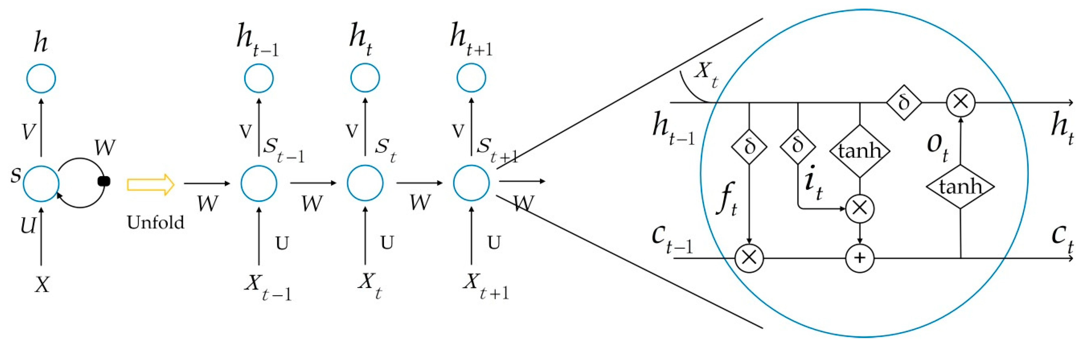
Figure 3.
Land Cover Classification Model Based on the Bi-LSTM.

Figure 4.
Cultivated land cover percentage distribution.
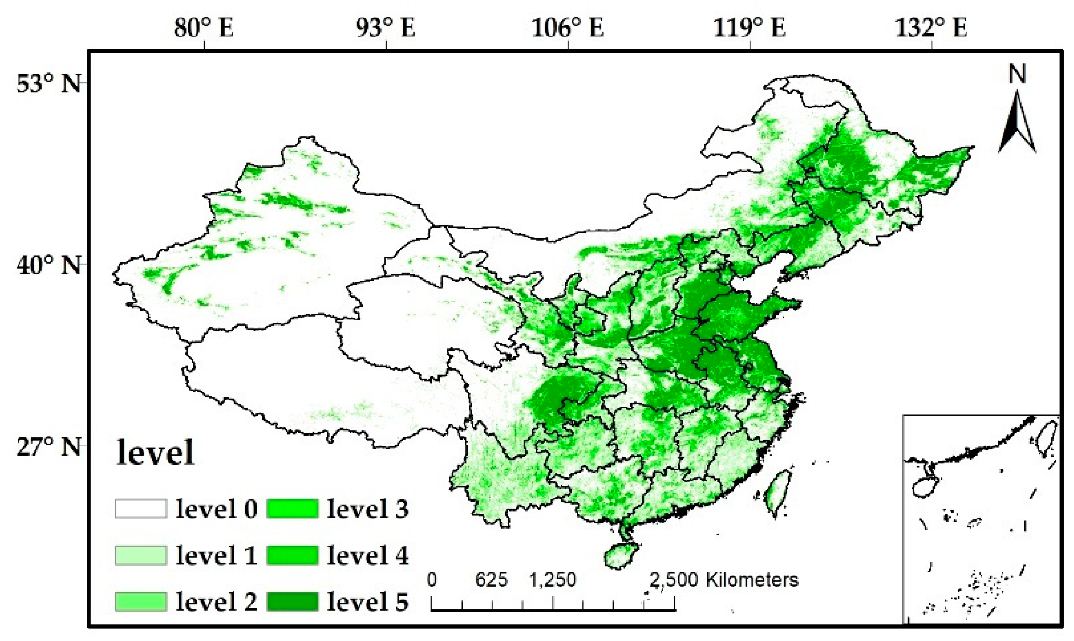
Figure 5.
Feature importance of 6 quantitative remote sensing features such as albedo, ET, FAPAR, GPP, LAI and NDVI obtained through random forest.
Figure 5.
Feature importance of 6 quantitative remote sensing features such as albedo, ET, FAPAR, GPP, LAI and NDVI obtained through random forest.
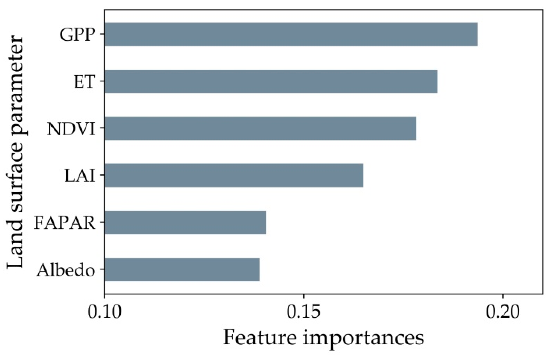
Figure 6.
Model training accuracy curve, validation accuracy curve and loss curve.

Figure 7.
Effect of the sample size on the model accuracy.

Figure 8.
Box diagram of each land cover type and the overall accuracy of the test set in 1980, 1990, 1995, 2000, 2005, 2010 and 2015. Crop (CR), Forest (FR), Shrubs (SR), Grass (GR), Water (WT), Glacier (GL), Wetland (WL), City (CT), Desert (DS), Tundra (TD) and OA (Overall).
Figure 8.
Box diagram of each land cover type and the overall accuracy of the test set in 1980, 1990, 1995, 2000, 2005, 2010 and 2015. Crop (CR), Forest (FR), Shrubs (SR), Grass (GR), Water (WT), Glacier (GL), Wetland (WL), City (CT), Desert (DS), Tundra (TD) and OA (Overall).
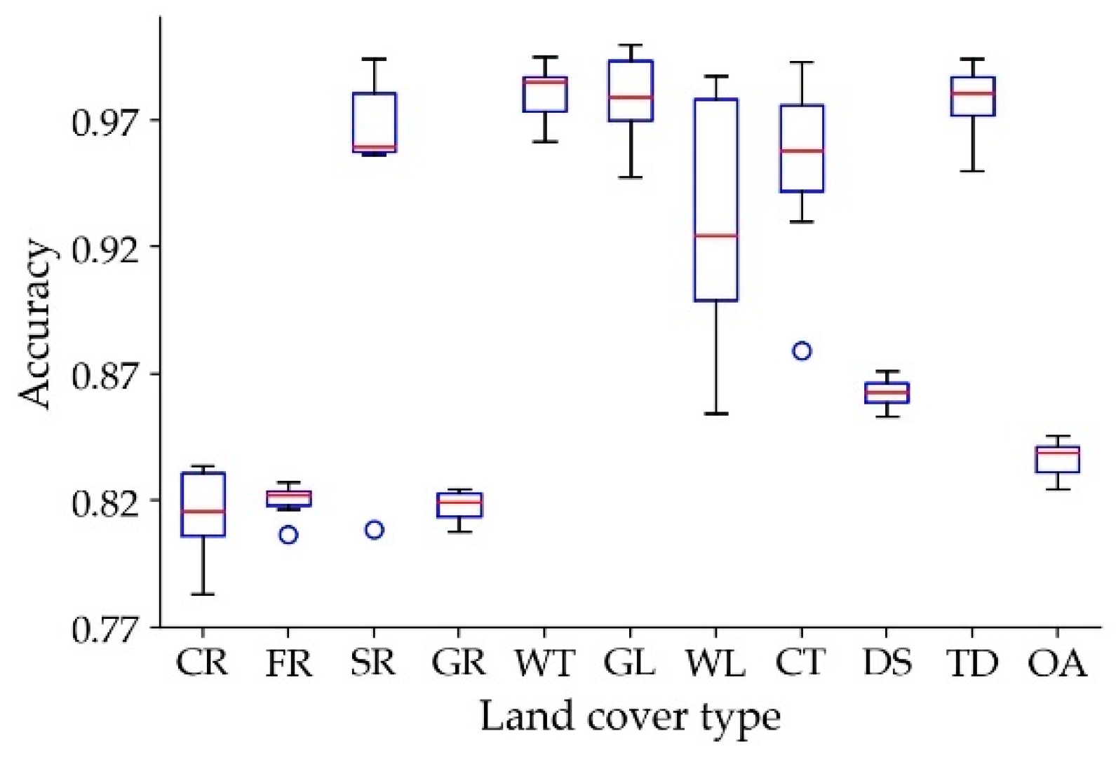
Figure 9.
Differences in time series between six quantitative remote sensing products in 10 categories.
Figure 9.
Differences in time series between six quantitative remote sensing products in 10 categories.

Figure 10.
Characteristic importance of each category.
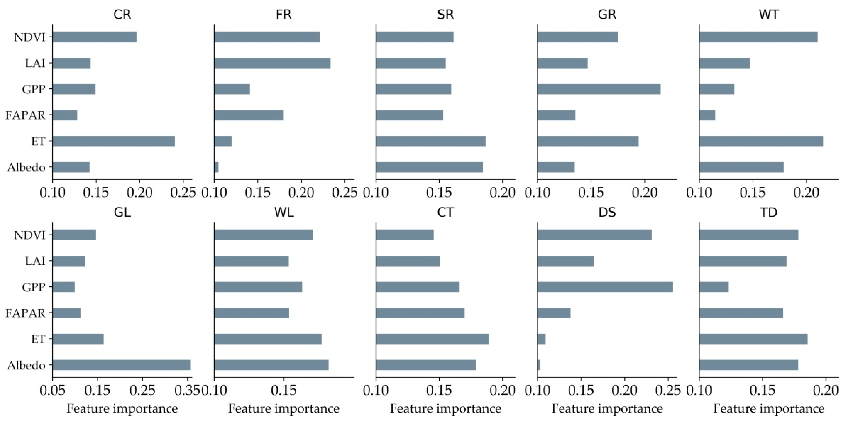
Figure 11.
(a) The CNLUCC original classification data, (b) the use of the stratified SMOTE algorithm, (c) the use of the SMOTE algorithm and (d) No use of the SMOTE algorithm. (e) Column contrast comparison, with an accuracy improvement of more than 20% and (f) large sample (Sample size is greater than 90 k) and small sample (Sample size is less than 90 k) category accuracy improvement trend chart.


Table 1.
Training set and test set.
| Class | Reliable Samples | Training Samples | Test Sample |
|---|---|---|---|
| Crop (CR) | 525,925 | 420,000 | 52,595 |
| Forest (FR) | 564,970 | 420,000 | 56,499 |
| Shrubs (SR) | 101,952 | 99,952 | 9484 |
| Grass (GR) | 869,197 | 630,000 | 86,823 |
| Water (WT) | 15,439 | 28,155 | 2818 |
| Glacier (GC) | 8363 | 15,850 | 1588 |
| Wetland (WL) | 9197 | 15,850 | 1537 |
| City (CT) | 5612 | 9282 | 931 |
| Desert (DS) | 310,044 | 420,000 | 53,584 |
| Tundra (TD) | 14,417 | 24,934 | 2464 |
Table 2.
Introduction to data used in this study.
| Data | Spatial Resolution | Time Resolution | Data Source |
|---|---|---|---|
| Albedo VIS | 0.05° | 16 days | GLASS |
| Albedo NIR | 0.05° | 16 days | GLASS |
| Albedo SHORT | 0.05° | 16 days | GLASS |
| ET | 0.05° | 16 days | GLASS |
| FAPAR | 0.05° | 16 days | GLASS |
| GPP | 0.05° | 16 days | GLASS |
| LAI | 0.05° | 16 days | GLASS |
| NDVI | 0.05° | 16 days | AVHRR |
| Nighttime-Lights | 0.05° | DMSP-OLS | |
| MERRA2 | 0.5° | 16 days | MERRA |
| DEM | 0.05° | 16 days | |
| Longitude | 0.05° | ||
| Latitude | 0.05° | ||
| Land cover | 0.05° | CNLUCC |
Table 3.
Comparison of the classification accuracies between different models and different quantitative remote sensing products.
Table 3.
Comparison of the classification accuracies between different models and different quantitative remote sensing products.
| Classifier Type | Input | Overall Accuracy | Mean F1-Score |
|---|---|---|---|
| Bi-LSTM | GPP only | 81.86% | 0.819 |
| NDVI only | 79.66% | 0.801 | |
| GPP + ET | 83.61% | 0.835 | |
| GPP + ET + NDVI | 84.93% | 0.848 | |
| GPP + ET + NDVI + LAI | 86.34% | 0.864 | |
| GPP + ET + NDVI + LAI + FAPAR | 87.21% | 0.872 | |
| GPP + ET + LAI + NDVI + FAPAR + Albedo | 88.04% | 0.878 | |
| GPP + ET + LAI + FAPAR + Albedo | 87.39% | 0.872 | |
| LSTM | GPP only | 79.13% | 0.793 |
| NDVI only | 75.23% | 0.758 | |
| GPP + ET + LAI + FAPAR + Albedo | 84.37% | 0.833 | |
| CNN | GPP only | 56.40% | 0.553 |
| NDVI only | 53.10% | 0.513 | |
| GPP + ET + LAI + FAPAR + Albedo | 72.35% | 0.716 | |
| SVM | GPP only | 63.73% | 0.611 |
| NDVI only | 60.58% | 0.601 | |
| GPP + ET + LAI + FAPAR + Albedo | 73.90% | 0.727 | |
| Random Forest | GPP only | 78.30% | 0.773 |
| NDVI only | 72.84% | 0.72 | |
| GPP + ET + LAI + FAPAR + Albedo | 79.83% | 0.793 |
Table 4.
Long time series land cover classification model precision confusion matrix.
| Reference Classes | Classified | ||||||||||
|---|---|---|---|---|---|---|---|---|---|---|---|
| CR | FR | SR | GR | WT | GC | WL | CT | DS | TD | ||
| Crop (CR) | 43,835 | 3366 | 814 | 3497 | 341 | 9 | 139 | 223 | 369 | 2 | 83.3% |
| Forest (FR) | 3359 | 47,280 | 2395 | 3011 | 43 | 14 | 94 | 42 | 174 | 19 | 83.7% |
| Shrubs (SR) | 301 | 821 | 7778 | 544 | 2 | 0 | 10 | 0 | 27 | 2 | 82.0% |
| Grass (GR) | 3185 | 3254 | 1521 | 72,173 | 212 | 165 | 217 | 32 | 5467 | 596 | 83.1% |
| Water (WT) | 82 | 20 | 0 | 55 | 2592 | 0 | 20 | 29 | 20 | 0 | 92.0% |
| Glacier (GL) | 0 | 8 | 0 | 21 | 0 | 1497 | 0 | 0 | 57 | 6 | 94.3% |
| Wetland (WL) | 41 | 22 | 13 | 19 | 7 | 0 | 1414 | 0 | 19 | 2 | 92.1% |
| City (CT) | 40 | 13 | 0 | 7 | 8 | 0 | 2 | 860 | 2 | 0 | 92.4% |
| Desert (DS) | 368 | 219 | 107 | 5787 | 111 | 332 | 88 | 29 | 46,179 | 363 | 86.2% |
| Tundra (TD) | 0 | 0 | 0 | 91 | 0 | 5 | 0 | 0 | 35 | 2332 | 94.6% |
| Overall | 84.2% | ||||||||||
Table 5.
Land cover percentage grading accuracy for 2010.
| Level 0 | Level 1 | Level 2 | Level 3 | Level 4 | Level 5 | Overall | |
|---|---|---|---|---|---|---|---|
| CR | 0.844 | 0.911 | 0.924 | 0.927 | 0.937 | 0.924 | 0.911 |
| FR | 0.844 | 0.911 | 0.924 | 0.927 | 0.937 | 0.924 | 0.911 |
| SR | 0.926 | 0.82 | 0.855 | 0.887 | 0.952 | 0.967 | 0.901 |
| GR | 0.777 | 0.902 | 0.881 | 0.869 | 0.854 | 0.967 | 0.875 |
| WT | 0.942 | 0.944 | 0.945 | 0.976 | 0.984 | 0.993 | 0.964 |
| GL | 0.995 | 0.945 | 0.972 | 0.971 | 0.980 | 0.976 | 0.972 |
| WL | 0.960 | 0.947 | 0.945 | 0.969 | 0.980 | 0.986 | 0.961 |
| CT | 0.945 | 0.914 | 0.948 | 0.968 | 0.961 | 0.976 | 0.951 |
| DS | 0.929 | 0.873 | 0.891 | 0.853 | 0.829 | 0.974 | 0.892 |
| TD | 0.993 | 0.955 | 0.955 | 0.965 | 0.969 | 0.930 | 0.963 |
Table 6.
SMOTE algorithm and stratified SMOTE algorithm precision comparison.
| Truth Value | SMOTE-Predicted | S-SMOTE-Predicted | SMOTE | S-SMOTE | ||
|---|---|---|---|---|---|---|
| CR | 75,749 | 63,996 | 65,220 | 84.5% | 86.1% | +1.6% |
| FR | 83,285 | 69,539 | 76,206 | 83.5% | 91.5% | +8.0% |
| SR | 13,893 | 9505 | 11,948 | 68.4% | 86.0% | +17.6% |
| GR | 117,764 | 94,265 | 104,928 | 80.0% | 89.1% | +9.1% |
| WT | 3911 | 2619 | 3555 | 67.0% | 90.9% | +23.9% |
| GL | 1336 | 925 | 1416 | 69.2% | 93.3% | +24.1% |
| WL | 2539 | 882 | 1978 | 34.7% | 77.9% | +43.2% |
| CT | 2238 | 803 | 2035 | 35.9% | 91.0% | +55.1% |
| DS | 81,293 | 64,517 | 75,829 | 79.4% | 93.3% | +13.9% |
| TD | 2201 | 1217 | 1983 | 55.1% | 90.1% | +35.0% |
© 2019 by the authors. Licensee MDPI, Basel, Switzerland. This article is an open access article distributed under the terms and conditions of the Creative Commons Attribution (CC BY) license (http://creativecommons.org/licenses/by/4.0/).
Share and Cite
MDPI and ACS Style
Wang, H.; Zhao, X.; Zhang, X.; Wu, D.; Du, X. Long Time Series Land Cover Classification in China from 1982 to 2015 Based on Bi-LSTM Deep Learning. Remote Sens. 2019, 11, 1639. https://0-doi-org.brum.beds.ac.uk/10.3390/rs11141639
AMA Style
Wang H, Zhao X, Zhang X, Wu D, Du X. Long Time Series Land Cover Classification in China from 1982 to 2015 Based on Bi-LSTM Deep Learning. Remote Sensing. 2019; 11(14):1639. https://0-doi-org.brum.beds.ac.uk/10.3390/rs11141639
Chicago/Turabian StyleWang, Haoyu, Xiang Zhao, Xin Zhang, Donghai Wu, and Xiaozheng Du. 2019. "Long Time Series Land Cover Classification in China from 1982 to 2015 Based on Bi-LSTM Deep Learning" Remote Sensing 11, no. 14: 1639. https://0-doi-org.brum.beds.ac.uk/10.3390/rs11141639
Note that from the first issue of 2016, this journal uses article numbers instead of page numbers. See further details here.