Article

Automated Near-Real-Time Mapping and Monitoring of Rice Extent, Cropping Patterns, and Growth Stages in Southeast Asia Using Sentinel-1 Time Series on a Google Earth Engine Platform

1
School of Food Science and Technology, Universiti Malaysia Terengganu, Kuala Nerus, Terengganu 21030, Malaysia
2
Faculty of Fishery and Food Sciences, Universiti Malaysia Terengganu, 21030 Kuala Nerus, Terengganu, Malaysia
3
School of Life & Environmental Sciences, Sydney Institute of Agriculture, The University of Sydney, Sydney, NSW 2006, Australia
4
Department of Civil and Environmental Engineering, IPB University (Bogor Agricultural University), Bogor 16680, Indonesia
*
Authors to whom correspondence should be addressed.
Remote Sens. 2019, 11(14), 1666; https://0-doi-org.brum.beds.ac.uk/10.3390/rs11141666
Submission received: 16 June 2019 / Revised: 8 July 2019 / Accepted: 10 July 2019 / Published: 12 July 2019
(This article belongs to the Special Issue Digital Mapping in Dynamic Environments)

Abstract

:
More than 50% of the world’s population consumes rice. Accurate and up-to-date information on rice field extent is important to help manage food and water security. Currently, field surveys or MODIS satellite data are used to estimate rice growing areas. This study presents a cost-effective methodology for near-real-time mapping and monitoring of rice growth extent and cropping patterns over a large area. This novel method produces high-resolution monthly maps (10 m resolution) of rice growing areas, as well as rice growth stages. The method integrates temporal Sentinel-1 data and rice phenological parameters with the Google Earth Engine (GEE) cloud-based platform. It uses monthly median time series of Sentinel-1 at VH polarization from September 2016 to October 2018. The two study areas are the northern region of West Java, Indonesia (0.75 million ha), and the Kedah and Perlis states in Malaysia (over 1 million ha). K-means clustering, hierarchical cluster analysis (HCA), and a visual interpretation of VH polarization time series profiles are used to generate rice extent, cropping patterns, and spatiotemporal distribution of growth stages. To automate the process, four supervised classification methods (support vector machine (SVM), artificial neural networks (ANN), random forests, and C5.0 classification models) were independently trialled to identify cluster labels. The results from each classification method were compared. The method can also forecast rice extent for up to two months. The VH polarization data can identify four growth stages of rice—T&P: tillage and planting (30 days); V: vegetative-1 and 2 (60 days); R: reproductive (30 days); M: maturity (30 days). Compared to field survey data, this method measures overall rice extent with an accuracy of 96.5% and a kappa coefficient of 0.92. SVM and ANN show better performance than random forest and C5.0 models. This simple and robust method could be rolled out across Southeast Asia, and could be used as an alternative to time-consuming, expensive field surveys.

Graphical Abstract

1. Introduction

Rice is a source of food for more than half of the global population [1]. Accurate and up-to-date information on rice field extent and cropping patterns can help:
  • tackle food security issues, especially in countries where rice is the major staple food;
  • identify and forecast rice production in a region;
  • manage water security, as paddy rice consumes a large amount of water [1];
  • with greenhouse gas accounting, as paddy rice releases methane (CH4) to the atmosphere [2];
  • form government policies.
The past decade has seen a rapid increase in the use of satellite-based remote sensing data to map and monitor paddy rice fields. This growth can be attributed to at least three factors—the availability of open remote sensing data, advanced machine learning methods, and access to cloud computing platforms that can handle big data storage and processing. Rice fields have been mapped using different data sources, including optical products (e.g., MODIS, Landsat, Sentinel-2, and SPOT) and Synthetic Aperture Radar (SAR) or microwave data (e.g., RADARSAT, ALOS PALSAR, and Sentinel-1). Recently, SAR-based images have gained attention because they are not affected by clouds or illumination conditions [3].
Time series images such as the Sentinel-1 data are now freely available. Sentinel-1A is the next generation of the C-band (center frequency: 5.405 GHz) radar sensor which was launched on 3 April 2014 and operated by the European Commission’s Copernicus Programme [4]. It was designed for continuous near-real-time land and ocean monitoring, and revisits the equator every 12 days. The launch of Sentinel-1B on 25 April 2016 is expected to double the revisit time. The Sentinel satellites provide dual-polarized (VV + VH) SAR images with a spatial resolution of 5 m × 20 m. Because of the excellent spatiotemporal coverage, resolution, and independence from cloud coverage, Sentinel-1 data are a valuable alternative to other satellite products, such as the multi-spectral, 250 m resolution, 16-day composite images from MODIS [5], or the combined MODIS/Landsat data [6].
Extensive research has been conducted on mapping and monitoring rice extent and rice verities using SAR backscatter data [7,8]. The potential of using Sentinel-1 to map rice extent and growing season has been investigated in various regions in the world, including Vietnam [9,10,11,12,13], China [14,15,16,17,18], USA and Spain [19], India [20,21,22,23], the Mediterranean region [24], Philippines [25], Thailand [23], and Myanmar [26]. In particular, studies [10,17] reported that the VH backscatter of Sentinel-1 is more sensitive to detecting rice growth than the VV backscatter.
Various algorithms (e.g., unsupervised and supervised classifiers, knowledge and phenology-based approaches) have been used to estimate areas of rice fields in a region [1,7,27,28]. For mapping rice cropping patterns, unsupervised classification of spectral data (i.e., ISODATA and K-means unsupervised classification) are frequently used [6,15,29,30,31,32,33]. Subsequently, similar cluster spectra identified by K-means can be grouped using hierarchical cluster analysis (HCA) [5,34]. An advantage of this combination (K-means with HCA) is that the generated clusters can represent a gradient of cropping schedules [5,34]. To identify cropping patterns from the generated clusters, visual inspection of clusters’ spectra are required. This manual identification is tedious and time consuming, thus automated classification of rice cropping pattern using machine learning models would be advantageous [14,35].
The ability to process multi-temporal satellite data has also become less complicated. The Google Earth Engine platform (GEE, www.earthengine.google.com) is one of the most promising developments for earth science data access and analysis [36,37]. It contains a multi-petabyte catalogue of satellite imagery including Landsat, Sentinels, and MODIS. It also provides scripting ability to access, operate and visualize such data in an easy and scalable manner. For example, Global Forest Watch (https://earthengine.google.com/case_studies/) uses GEE to monitor changes to the world’s forests [38]. Users can synthesise data from the past decade or receive alerts about possible new threats in near-real-time. Thus, GEE also has a high potential to apply in near-real-time mapping and monitoring of paddy rice extent and cropping patterns. In a recent study, temporal Sentinel-1 data in GEE were used to map rice extent in India [21,22]. However, these studies only distinguished between rice and non-rice areas, and early and late rice.
The objective of this study was to develop a rapid, accurate, and cost-effective methodology for near-real-time mapping and monitoring of rice growth extent and cropping patterns using an integration of temporal Sentinel-1 data, phenological parameters, and GEE. The approach used a combination of K-means clustering, hierarchical cluster analysis (HCA), and visual interpretation. This study also established automated rice cropping pattern mapping using machine learning algorithms including support vector machine (SVM), artificial neural networks (ANN), random forests, and the C5.0 classification models. Using rice phenological parameters, the method provided spatiotemporal distribution of growth stages as well as forecasting rice extent for two months. This novel approach was tested in two regions in Southeast Asia: the northern region of West Java in Indonesia (0.75 million hectares (ha)) and the Kedah and Perlis states in Malaysia (over 1 million ha). These regions were selected as they are centres for rice production in both countries.

2. Materials and Methods
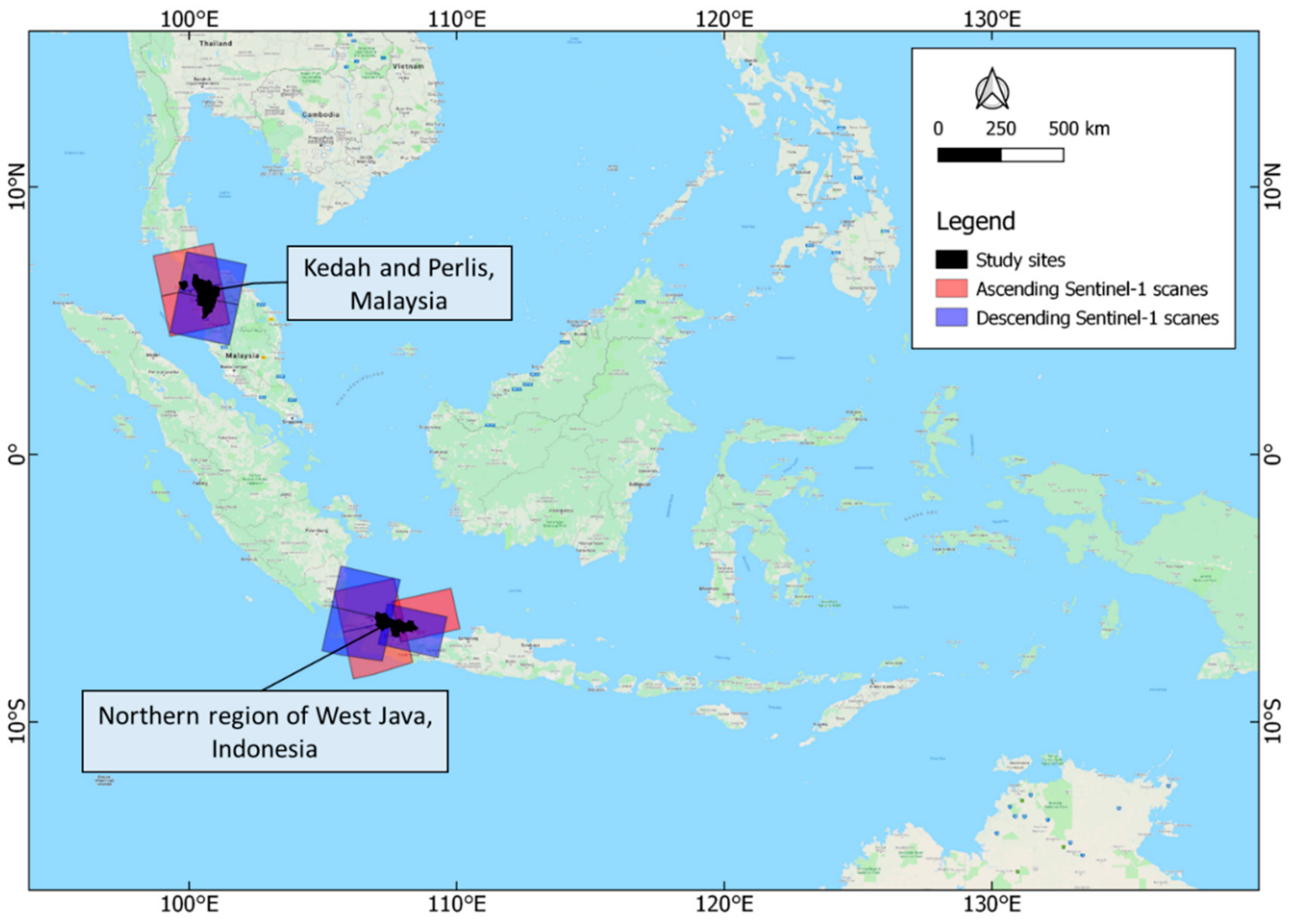
2.1. Study Sites

Study site 1 covers an area of 752,517 ha across four northern districts of West Java, Indonesia—the Indramayu, Subang, Karawang, and Bekasi districts (5.91°–6.85°S and 106.97°–108.54°E) (Figure 1). This area is Indonesia’s main rice production region [39]. The total rice field area in these four regencies is about 351,900 ha [40]. The area has a humid tropical climate with two seasons: wet and dry [41]. Wet season is from November to April; while dry season is from May to October [42]. Average annual rainfall is about 2000 mm [3]. Maximum average monthly rainfall is 272 mm (January), and minimum average monthly rainfall is 23 mm (August) [42]. The topography is almost flat [5].
Study site 2, in Malaysia, crosses the Kedah and Perlis states (5.08°–6.72°S and 99.64°–101.13°E) and covers about 1,024,800 ha (Figure 1). Rice fields are mostly located in the floodplain of the Padang Terap River with elevation ranging from sea level up to about 15 m a.s.l. [43]. Small areas of rice fields are also found in Langkawi Island which is a part of Kedah state. The region is classified as tropical rainforest [44] with an average rainfall of 2000 mm/year [45]. The highest monthly rainfall is about 350 mm in October. The driest months are December to March, with about 75 to 150 mm/month of rainfall [45]. The total rice paddy area in this study site is about 133,305 ha and is the largest grain growing area in Malaysia [46].

2.2. Farming Practices

Rice fields in study area 1 are irrigated and have a double rice cropping pattern [5]. Planting in the wet season (October to March) is known locally as “rendeng”. Planting during the dry season (April to September) is known locally as “gadu” [5]. As irrigation water is available year-round, farmers can grow rice in any month [47]. Between wet and dry season planting, rice fields are used to grow cash crops (e.g., maize, watermelon, groundnut) or left fallow to halt the propagation of pests and diseases [5]. The main rice varieties used by farmers in the Subang district, during the wet season, are Ciherang (116–125 days), Inpari, Mekonga (120 days), Sintanur (115 days), IR42 (135 days), and Ketan (135 days) [47].
The rice fields in study site 2 are also irrigated and have a double rice cropping pattern [46]. The planting seasons are divided into a main season with a wet paddy rice crop (September to March), and an off-season rice crop (April to September) [46]. These are locally known as “tanaman musim utama” and “tanaman luar musim”, respectively. Popular rice varieties that are planted in site 2 include MR220 CL2 (97–113 days), Padi Siraj MARDI 297 (105–110 days), MR263 (97–104 days), and MR219 (105–110 days) [48,49].

2.3. Datasets

2.3.1. Sentinel-1 Data and Pre-Processing

For rice mapping, the VH polarization of Sentinel-1 gives more valuable information than VV polarization [10]. As such, VH polarization data from September 2016 to October 2018 were used for both study sites. The data had a spatial resolution of 10 m in interferometric wide swath (IW) mode and ground range detected (GRD) format, and was collected from both orbital directions (ascending and descending). Study site 1 had 321 Sentinel-1 scenes from GEE, while study site 2 had 405. Only Sentinel-1A data were used as Sentinel-1B data was not available in both study areas.
The data were pre-processed by GEE within the Sentinel-1 Toolbox, including orbital correction, thermal noise removal, radiometric calibration, and terrain correction (orthorectification). A median filter was applied to obtain monthly Sentinel-1 layers using the imageCollection.median() function in GEE. This filter was used to reduce the amount of noise, especially at the border between scenes, as the sites are covered by six (site 1) and four (site 2) different scenes (Figure 1). Monthly image compositing was also required as each scene in the study sites was acquired at a different time.

2.3.2. Reference Data
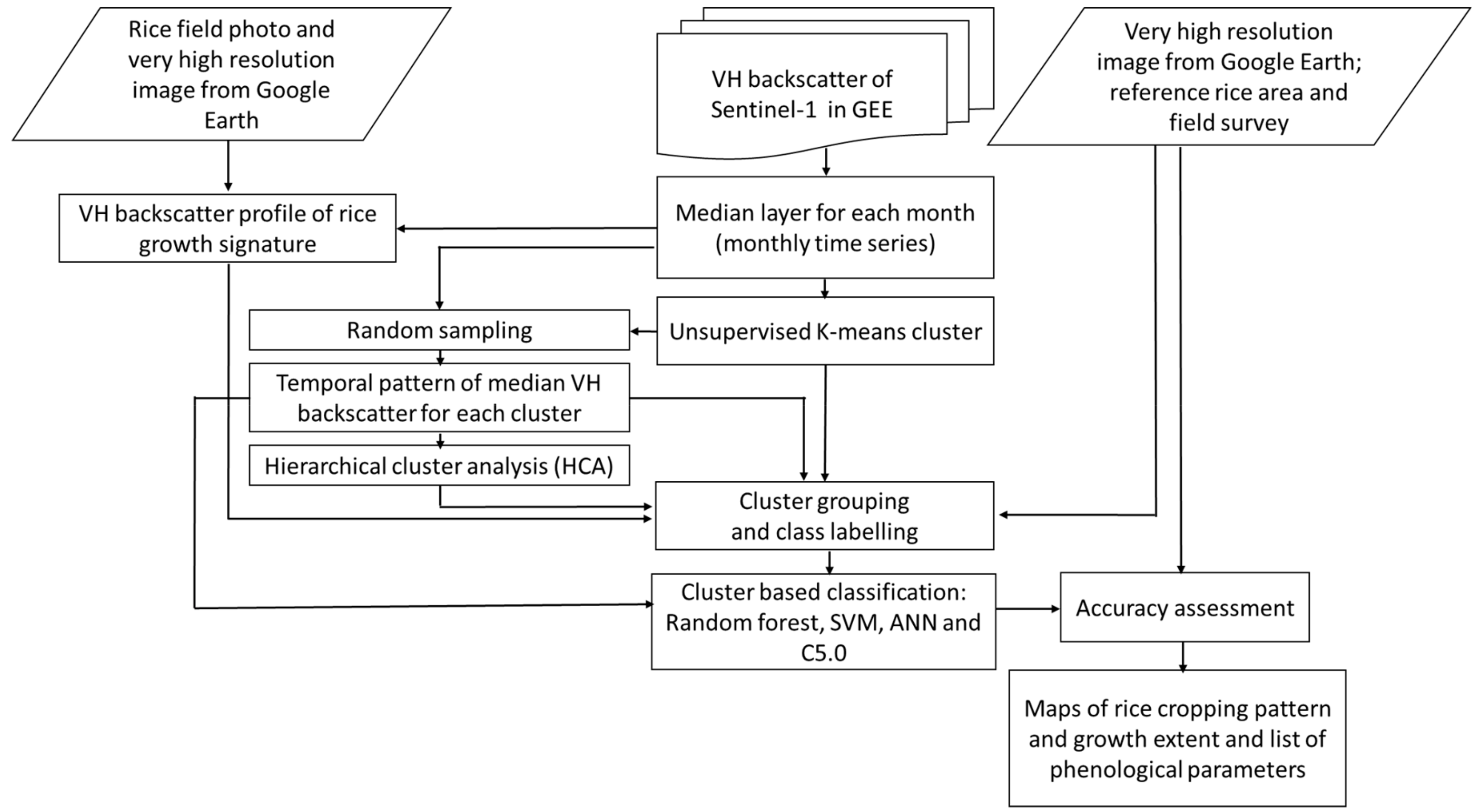
At site 1, a camera was installed in the Indramayu district (at 6.4275°S, 108.1085°E) to take daily photos from May 2017–February 2018. The photos were used to gather ground-truthed phenological information of rice and water conditions in the field during the growing season. The very high resolution (VHR) images from Google Earth (resolution of 15–30 cm [50]) were also used as reference data for differentiating rice and non-rice areas. Survey data on rice field extents were obtained from the provincial government statistical agency [40]. Rice cropping calendars were obtained from the previous study of [5].
At study site 2, VHR images from Google Earth (resolution of 15–30 cm [50]) were used to differentiate rice and non-rice areas. There was no camera at site 2. Rice cropping calendars and data on rice field extents were gathered from Department of Agriculture Peninsular Malaysia [46].
Administrative boundaries at the district level at site 1, and state levels at site 2, were obtained from ESRI shapefiles from http://www.diva-gis.org/gdata.

2.4. Methodology

Figure 2 presents the methodology for this study, and comprises the following steps:
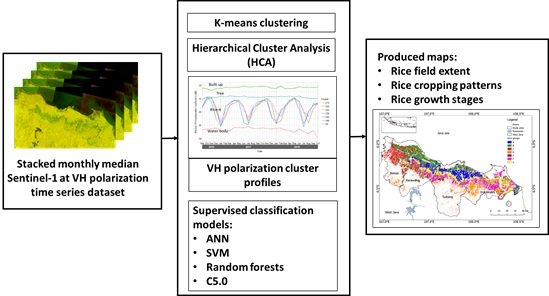
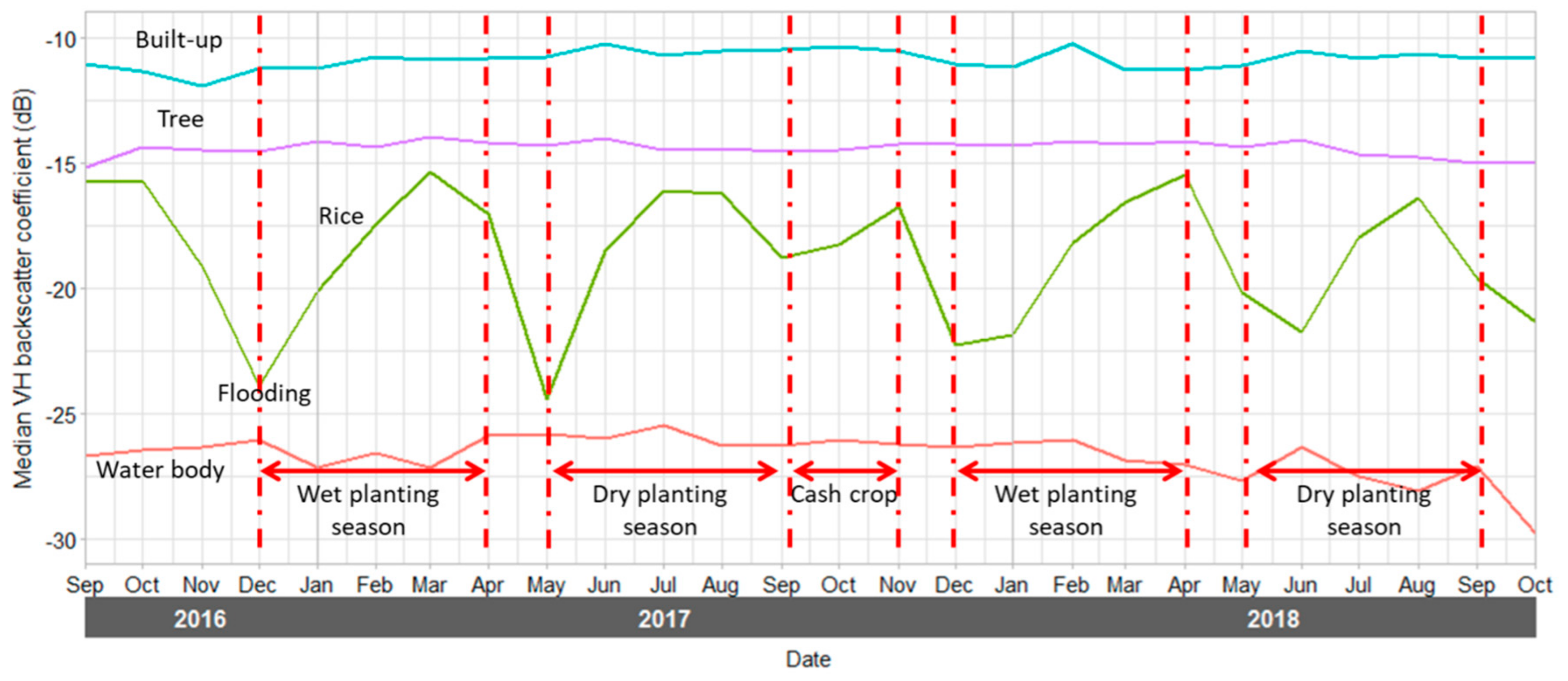
  • Monthly median Sentinel 1 VH polarization time series data were extracted for rice fields and non-rice areas at both study sites.
  • These monthly time series were sampled and classified using the K-means clustering method in GEE, resulting in 50 time series profile clusters.
  • The spatial median of the VH polarization time series profiles was extracted for each cluster as a representative VH polarization profile.
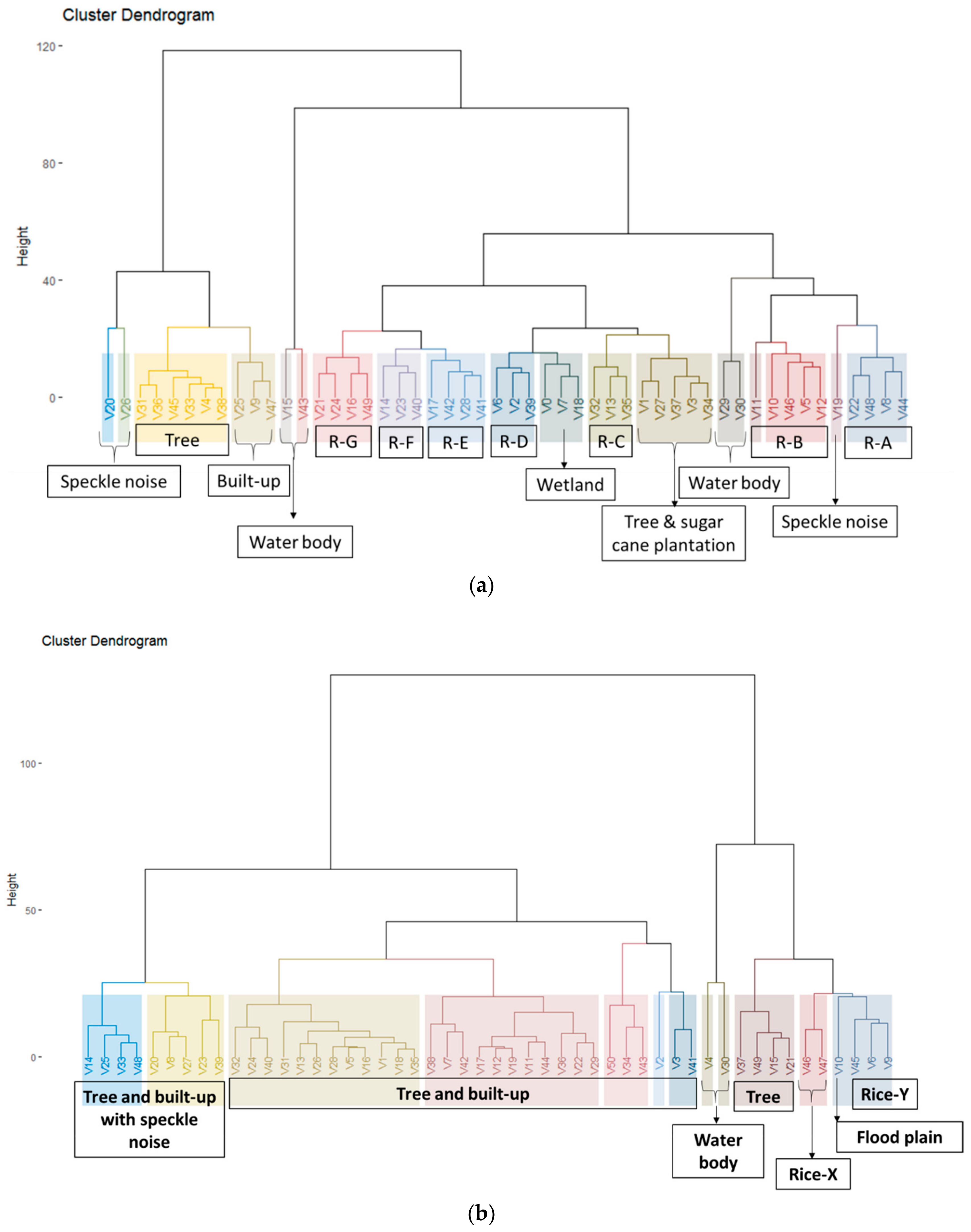
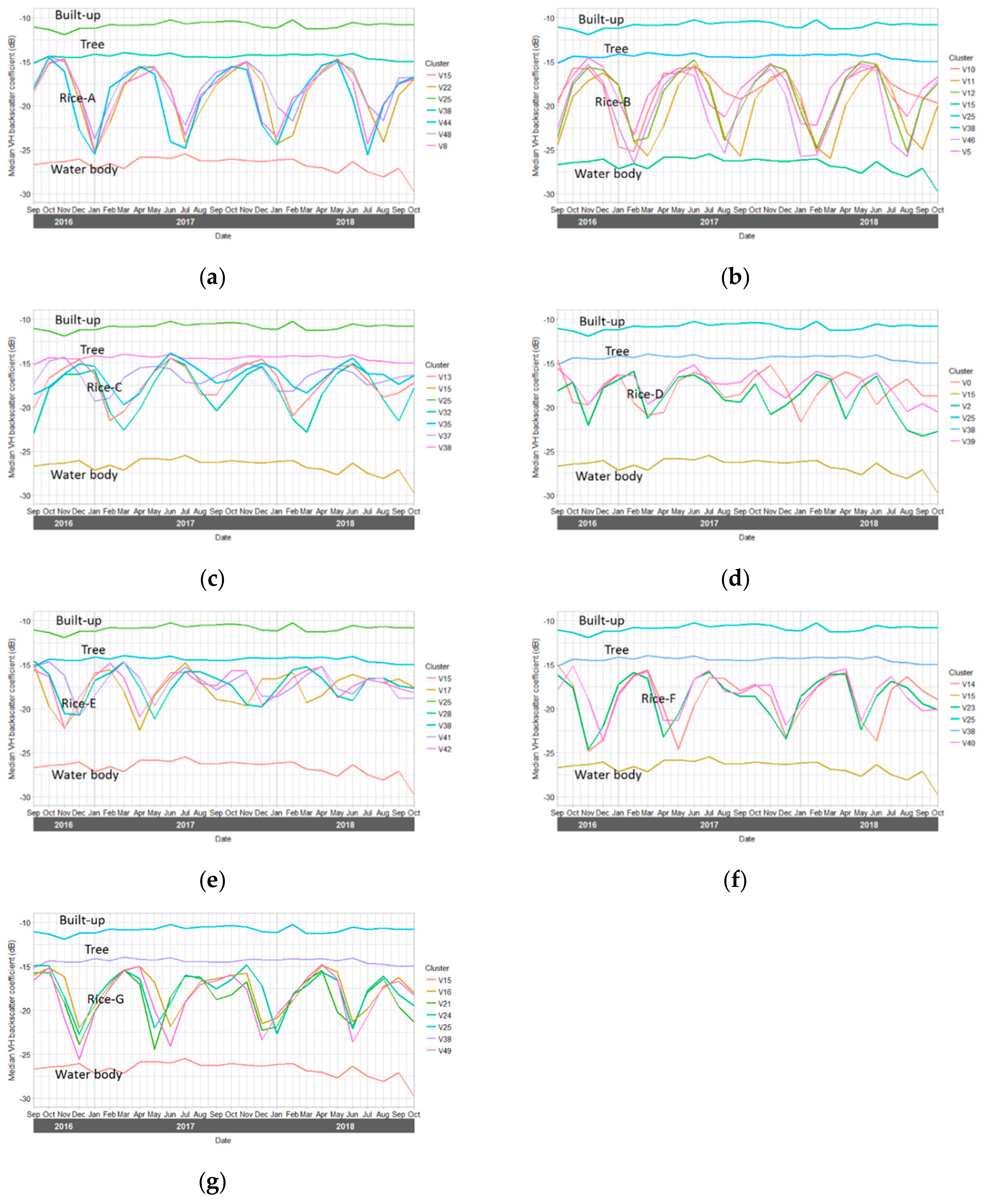
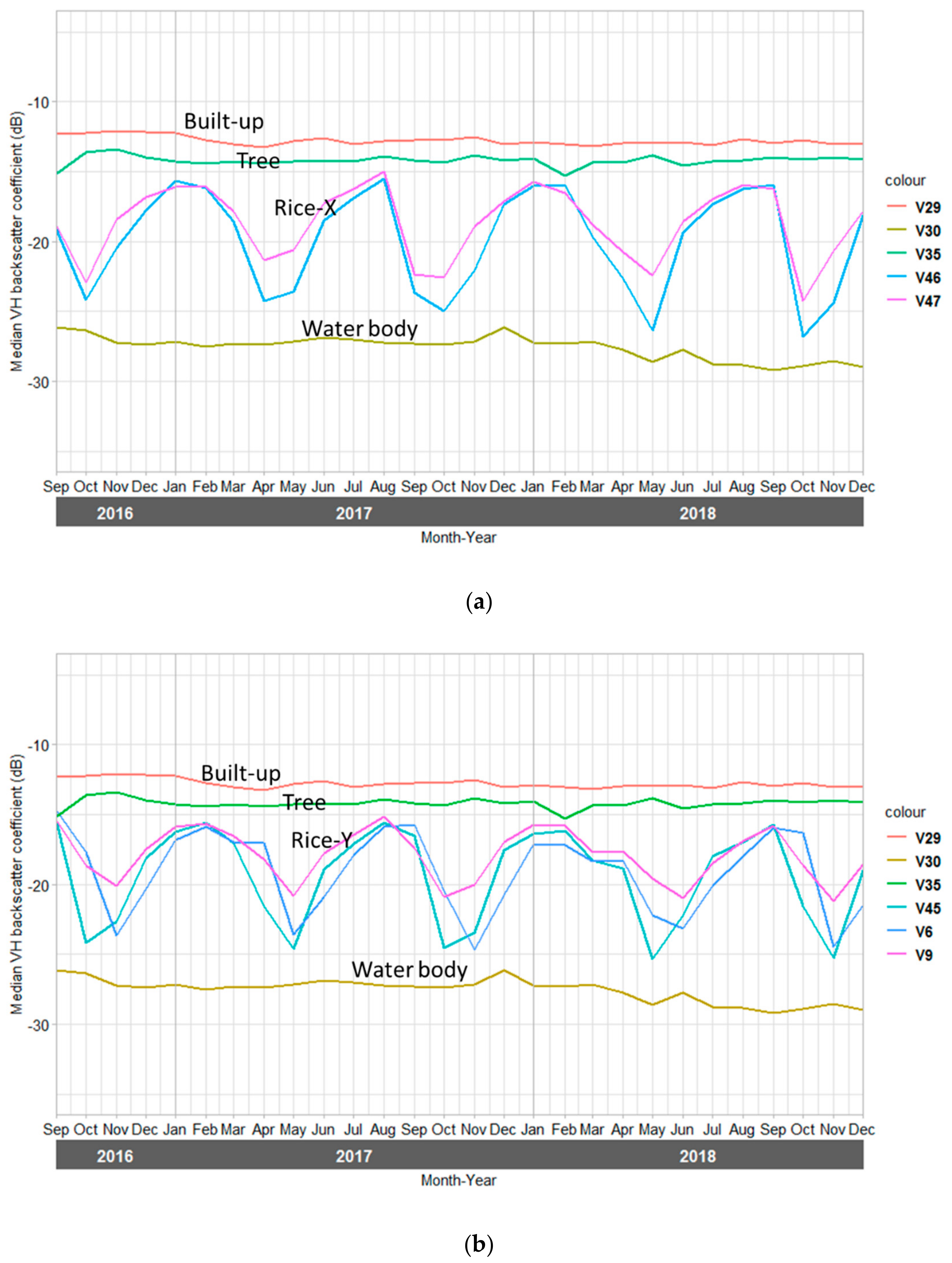
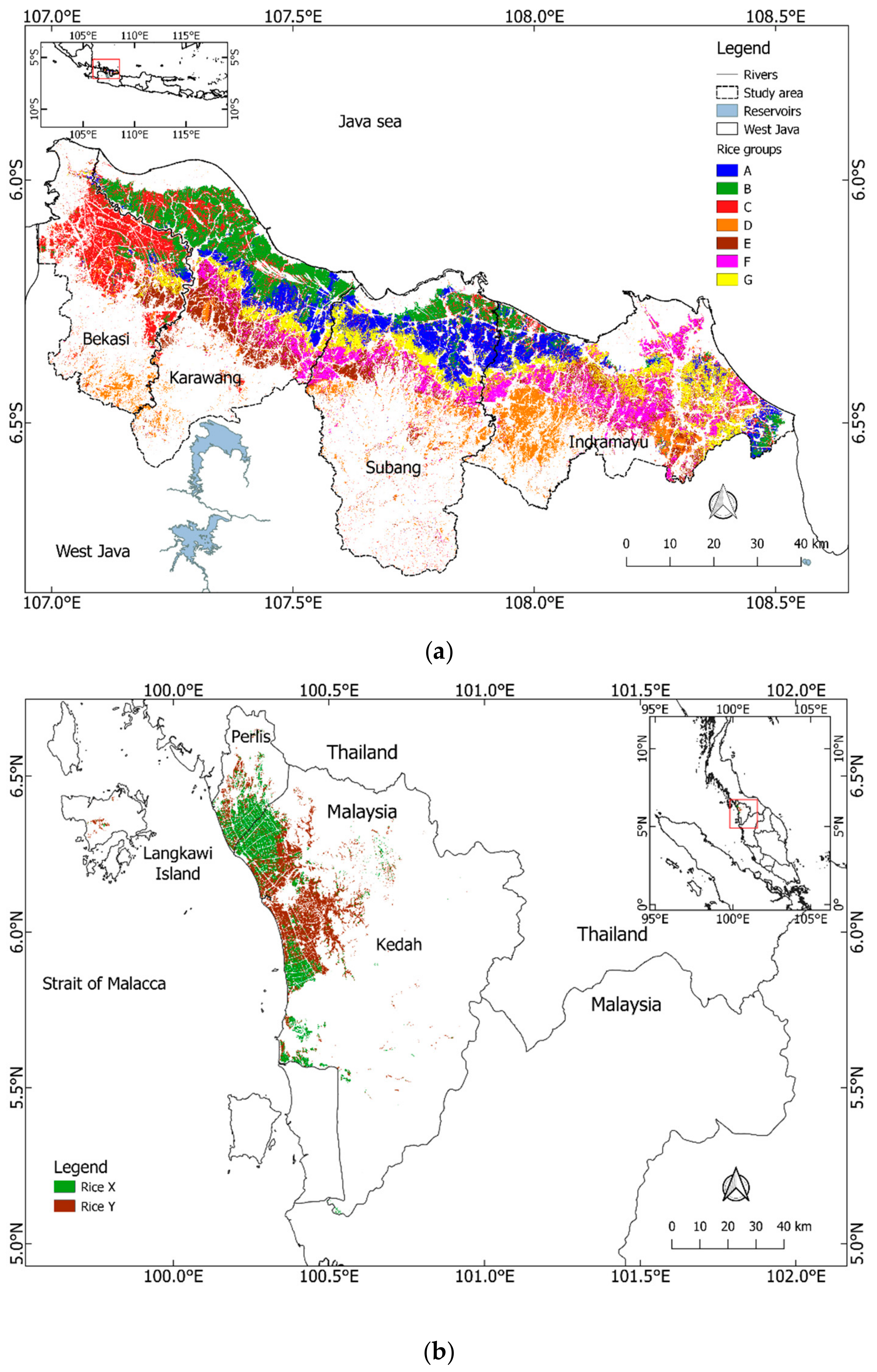
  • Clusters were then grouped using hierarchical cluster analysis (HCA), based on the similarities of the representative VH polarization cluster profiles. This grouping resulted in seven rice units (rice group A, B, C, D, E, F and G) at site 1 (see Figure 5a and Table S1), and two rice units (rice group X and Y) at site 2 (see Figure 5b and Table S2).
  • Rice cropping patterns were identified based on the representative VH polarization profile of each cluster.
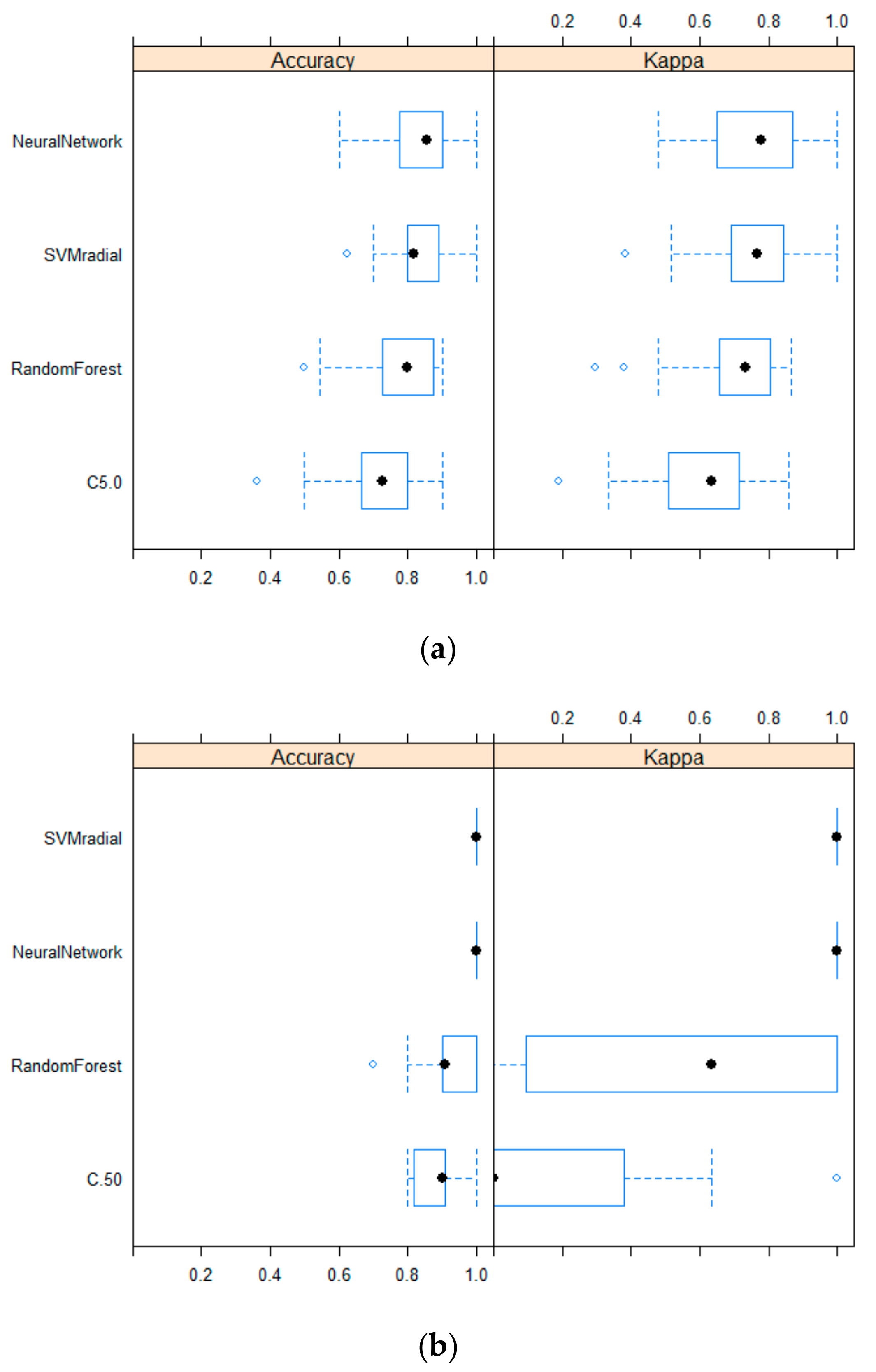
  • Automated mapping of rice cropping patterns in cluster levels was established using four different machine learning algorithms: SVM, ANN, random forests, and C5.0 classification models. The machine learning methods classified VH polarization profiles into defined rice units (growth stages).
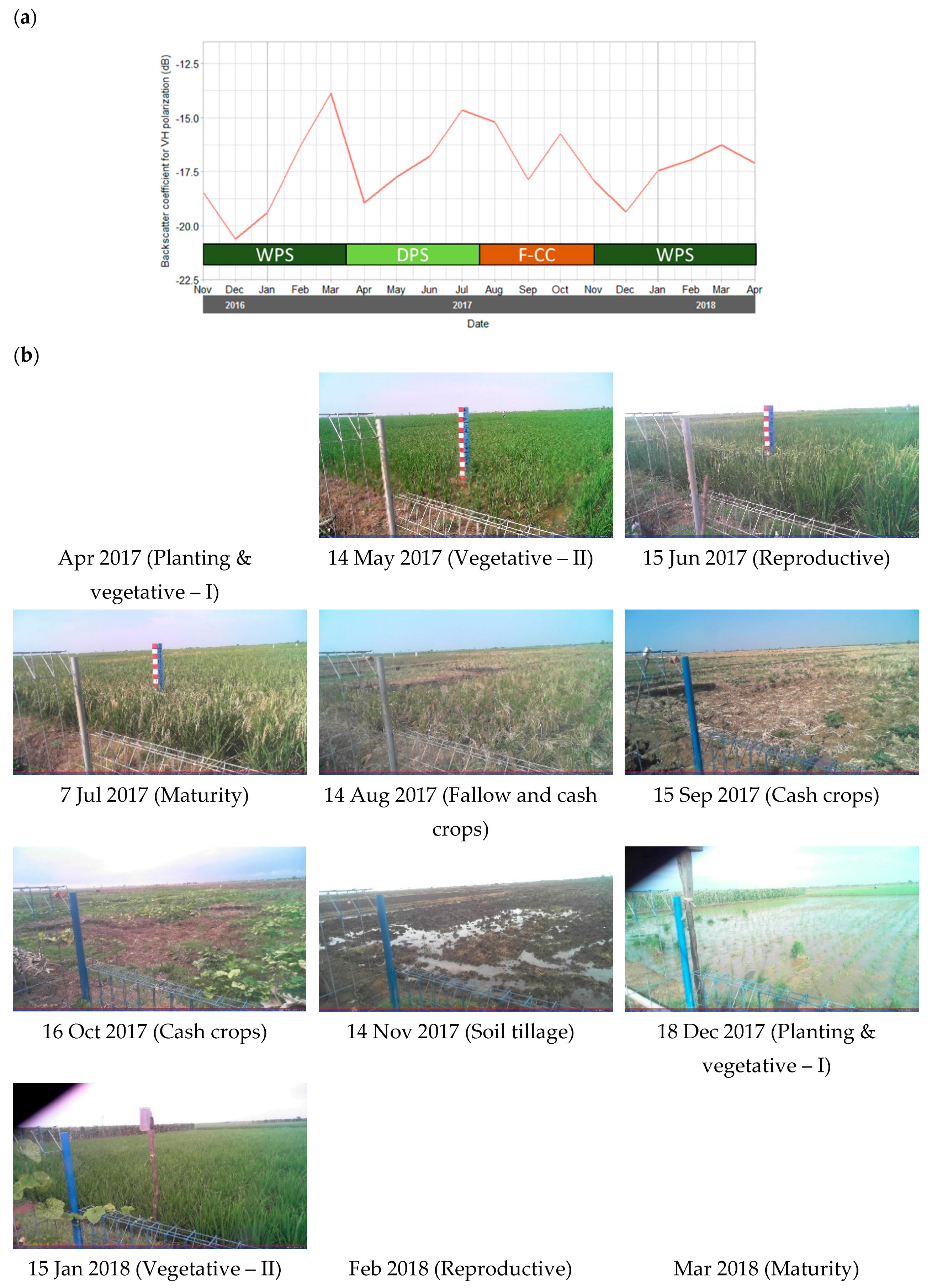
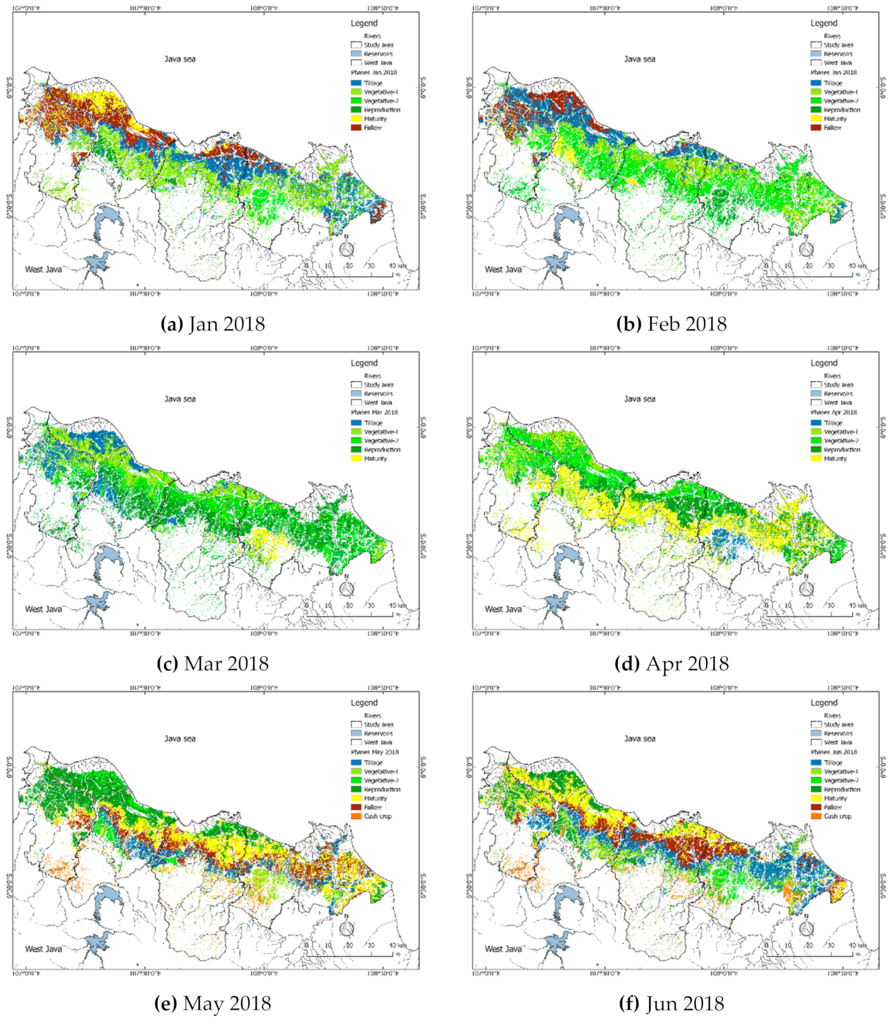
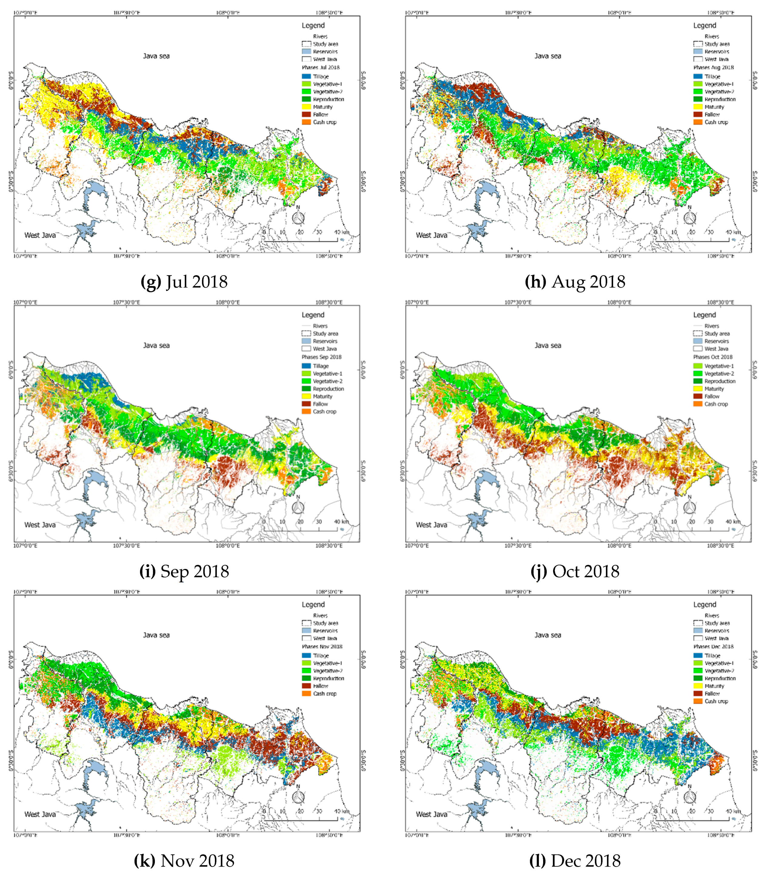
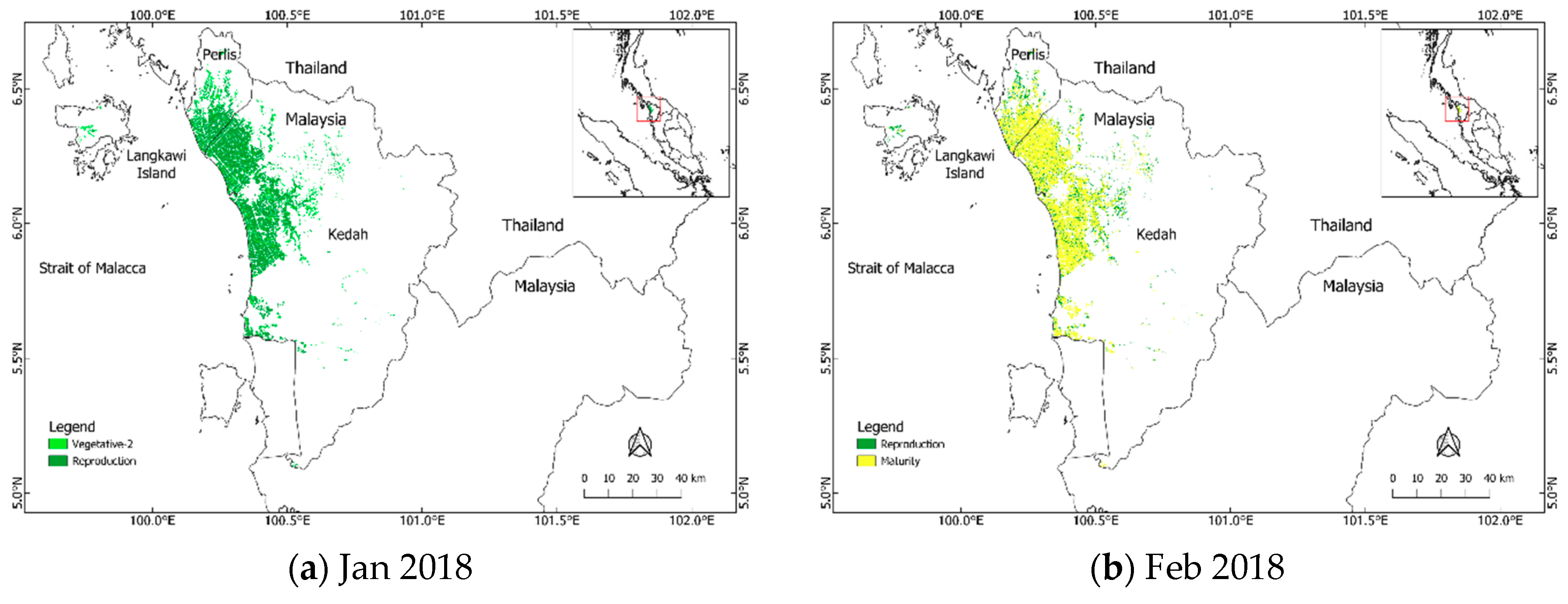
  • Rice phenological parameters (tillage and planting, vegetative, reproduction and maturity time) were identified from the representative VH polarization profiles of each rice cluster to determine monthly extents of growth stages.
Finally, the accuracy of the produced rice field extent was assessed using VHR images and compared with rice field areas derived from local and national survey data.

2.4.1. Analyzing the Time Series Profile of VH Polarization

Figure 3 shows the time series of Sentinel-1 backscatter VH polarizations at site 1 (West Java) and the corresponding field photos. The photos show that rice fields at the field router location have a double rice cropping pattern, where the first and second planting seasons (December to March and April to August) were referred to as wet and dry planting seasons, respectively. After the dry season harvest, and before wet season planting, the rice field was used for cultivating a cash crop (watermelon).
Figure 4 shows the time series of VH polarizations for four land-cover classes: rice field, waterbody, tree, and built-up. The rice fields have a distinct time series profile where the VH polarization values fluctuate seasonally while on other land covers the values are relatively constant. The VH polarization value for waterbody is about −26 dB, a tree about −14 dB, and built-up areas about −12 dB. Similar values were found in other studies [16,17,18,19].
The VH polarization time series, as shown in Figure 3 and Figure 4, were used to distinguish between rice growth stages. The time series can be related to the four designated rice cropping phenology groups—T&P: tillage and planting (30 days); V: vegetative-1 and 2 (60 days); R: reproductive (30 days); M: maturity (30 days). Thus, one season of rice cropping takes about 150 days or 5 months. At planting, when the land was tilled and flooded, the rice fields had a local minimum VH polarization value of about <−18 dB (i.e., close to the value of water body). Note that this value depended on water level or soil moisture during soil tillage. Higher water level leads to more negative VH values. The VH polarization value rapidly increased during vegetative growth and generative stages, peaking at the end of the generative stage when the crop entered the heading or maturity stage. The difference between the local minimum and the peak is about five months, representing one growing season. The polarization value decreased during fallow. Between seasons, a VH polarization value greater than −18 dB signified the beginning of cash crop cultivation.

2.4.2. Classifying Time Series of VH Polarization

The Sentinel-1 time series images (monthly layers from September 2016–October 2018 = 26 layers stack) were classified using the K-Means unsupervised classification method in GEE. This unsupervised classification method was used due to the large study area size, and diverse land uses and cropping patterns. The ee.Clusterer.wekaKMeans() function was used. The algorithm automatically normalizes numerical input attributes and uses the Euclidean distance to measure distances between clusters, with the objective to minimize within cluster variation (distances).
The K-Means model was built based on 10,000 random sampling points as representative pixels from the images. The model was used to predict clusters in the image collection at each site. The number of clusters was set at 50. This number of clusters was chosen to represent land uses in the area (rice field, waterbody, built-up, tree) because a low number of clusters can lead to a loss of important information and less accurate analysis [5,30,51].

2.4.3. Extracting Representative VH Polarization Cluster Profiles

To interpret the land cover and rice units identified by the clusters, we generated representative VH polarization time series profiles for each cluster. Sampling points (n = 2500) were randomly generated from the images and uploaded and stored in Google Fusion Tables. To generate the representative VH polarization cluster profiles, spatial median values of the monthly time series were derived for each cluster using the “median aggregate” function in R software [52].

2.4.4. Grouping and Labelling Clusters

Some of the clusters established by the K-means method were similar, and thus the clusters were grouped based on their similarities of VH polarization profiles. To establish a natural gradient grouping, VH polarization cluster profiles were grouped using the HCA in R software [52] using the factoextra package. The Ward D2 method with the Euclidian distance was applied. The result of the HCA is presented as a dendrogram and shown in Figure 5a for site 1 and Figure 5b for site 2.
Subsequently, median VH polarization profiles for every cluster were inspected visually to identify each cluster whether it was belonging rice field or non-rice field (e.g., water bodies, built-up and tree). For site 1, 27 out of 50 clusters were identified as rice fields (see Figure 6) and grouped into seven rice units (Figure 5a) as follows:
  • Rice field A (grouping cluster V22, V48, V44 and V8),
  • Rice field B (grouping cluster V11, V10, V46, V5 and V2),
  • Rice field C (grouping cluster V32, V13, and V35),
  • Rice field D (grouping cluster V6, V2 and V39),
  • Rice field E (grouping cluster V17, V42, V28 and V41),
  • Rice field F (grouping cluster V14, V23 and V40), and
  • Rice field G (grouping cluster V21, V24, V16 and V49).
For site 2, only five out of 50 clusters were identified as rice fields (see Figure 7) and were grouped into two rice units (Rice field X and Y) (Figure 5b) as follows:
  • Rice field X (grouping cluster V46 and V7), and
  • Rice field Y (grouping cluster V49, V6 and V9).
These units correspond to different rice cropping phenological stages, and will be discussed in Section 3.1.
Additionally, Figure 5a also shows three clusters that were identified as noises in VH polarization cluster profiles at site 1. At site 2, nine clusters were identified as noises (Figure 5b).

2.4.5. Models for Automated Rice Cropping Pattern Mapping

Since rice fields change seasonally, it was assumed that the representative VH polarization profiles also replicated annual rice field characteristics and occurred in clusters. Thus, to automatically generate rice cropping pattern maps (i.e., rice units A, B, C, D, E, F and G at site 1 and rice unit X and Y at site 2), supervised classification sorted the clusters into rice units based on the representative VH polarization profiles. Four different algorithms: support vector machine (SVM), artificial neural networks (ANN), random forests, and C5.0 classification models were trialled independently and compared.
SVM classification was conducted using the kernlab R package [53]. The C-SVM classification algorithm with the Gaussian radial basis function was selected. Two parameters: σ and C were tuned with σ = [0.005, 0.01, 0.025, 0.05, 0.075, 0.1, 0.2] and C = [2 : 5].
ANN classification was performed using the nnet R package [54]. ANN consisted of three layers: input, hidden and output layers. The nodes were connected from input to hidden layers, hidden to output layers, and bypass connected from input to output layers. The number of nodes in hidden layers (size) and decay parameter values were tuned with size = [5,10,15,20] and decay = [0.01, 0.1, 0.25].
Random forests for classification was carried out using RandomForest R package [55]. The number of trees to grow was set at 500 as a default value. Only one parameter, the number of variables randomly sampled as candidates at each split (mtry) was tuned with mtry = [1 : 10].
The C5.0 classification model was performed using C5.0 [56] R packages [57]. Model type (classification tree models or rule-based models), number of boosting iterations (trials), and winnowing (i.e., feature selection) (whether it is used or not) were tuned with trials = [1 : 10].
For tuning parameters in the four supervised classification models, 5-fold cross-validation was used and repeated five times. The tuning parameters were conducted using the caret R package [58] with a grid search method. Overall accuracy (%) and the kappa coefficient were used to evaluate model performance.

2.4.6. Extracting Phenological Parameters

Rice phenological parameters, including the starting season and the length of the growing season, were manually extracted for each of the rice field clusters from Figure 6 (site 1) and Figure 7 (site 2). Then, based on the start of the growing season, rice growth stages were allocated to one of the designated growth stages (T&P, V-1, V-2, R, M). Note that every stage was assumed to last for a month. Once the local minimum of the VH polarization cluster profile was identified as tillage and planting (see Section 2.4.1), the proceeding growth stages (i.e., V-1, V-2, R, and M) were readily determined. Tables S1 and S2 present list of rice cropping phenological stages for site 1 and 2, respectively.

2.4.7. Accuracy Assessment

The accuracy of the rice field extents was evaluated using three types of data: (1) validation using the VHR images, (2) comparison with the government statistics of rice field area and (3) comparison with the known planting and harvesting schedule.
The reference data from VHR images—with a resolution of 15–30 cm [50]—were obtained from Google Earth by generating 500 random points within the study area. This assessment was conducted at the pixel level. From the 500 points, 199 points were visually identified as rice fields and 301 points were identified as non-rice (tree, water body and built-up) for site 1. For site 2, 59 points were identified as rice fields and 441 points were identified as non-rice. The accuracy of the rice field map was then evaluated using a confusion matrix and kappa analysis.
The accuracy of the rice field extents was also evaluated at the district level from the West Java provincial statistic agency for site 1, and at the state level of Kedah and Perlis from Department of Agriculture Peninsular Malaysia [46] for site 2. Note that this data was compiled from field surveys. Root mean square error (RMSE) and R2 were used to compare and to measure the accuracy of the maps from this study with the government data.
To assess temporal accuracy, planting schedules were compared with reference data from the previous study of [5] and Department of Agriculture Peninsular Malaysia [46] for the first and second study sites, respectively.

3. Results

3.1. Map of Rice Extent and Cropping Patterns

Figure 8a presents the rice extent and cropping patterns at site 1. The cropping phenological parameters of growth stages for each of the rice field clusters from September 2016 to October 2018 are listed in Table S1. The results show that rice fields in the study area have a double cropping system. From September 2016 to October 2018, the start of season ranges from November to March for the wet planting season and March to September for the dry planting season. Note that crops were planted in every month except for October. After the dry planting season, cash crop cultivation was detected in rice field C, D, E, F and G. Areas in fallow were identified by clusters that did not show tillage or another rice stage for a period of 1–2 months.
The rice field units at site 1 were characterized by elongated horizontal shapes representing the gradient of rice cropping schedules. This pattern was also reported by [5,47]. As shown in Table S1, the planting season started in the south and progressed north to the coast as the season advanced (starting from rice field D, then E, F, G, A, B to C), following the release of irrigation water from the Ir. Djuanda reservoir. Consequently, rice field clusters that are close to the coastal areas were planted later and classified as late rice groups (rice field A and B).
Figure 5a also shows the similarities of the VH polarization cluster profiles within the rice units at site 1. Rice units D and E were located at a higher elevation and have a larger within-cluster variation compared to rice units located in lowlands. This indicates that rice fields located at higher elevations have a larger variation in planting schedules, likely because of the lack of irrigation water.
At site 2, Figure 8b shows that most rice fields are concentrated in the MADA granary (around Alor Setar, the capital city of Kedah state). It also shows that only two rice units (rice field X and Y) were generated when the five clusters were grouped (see Figure 5b). Table S2 outlines crop growth stages derived from the crop phenological parameters for each cluster. Rice field X is located in the northern and southern part of the MADA granary area, while rice field Y covers the central part of MADA as well as a small part of Langkawi Island. Both rice groups are typically double cropping pattern without cash crops. Rice field X was planted earlier than rice field Y, and planting times reflect irrigation water availability. Rice field X was planted in October for the main season and April to May for the off-season. Rice field Y was planted in November for the main season and May to June for the off-season.
One notable difference between the sites is the complexity in rice cropping patterns. Although irrigated fields at both study sites have two rice crops a year (double rice cropping), site 1 has 7 rice pattern units while Site 2 only has two rice pattern units. Additionally, cash crops are sometimes grown at site 1 between the wet and dry planting seasons, while only rice is grown at site 2.

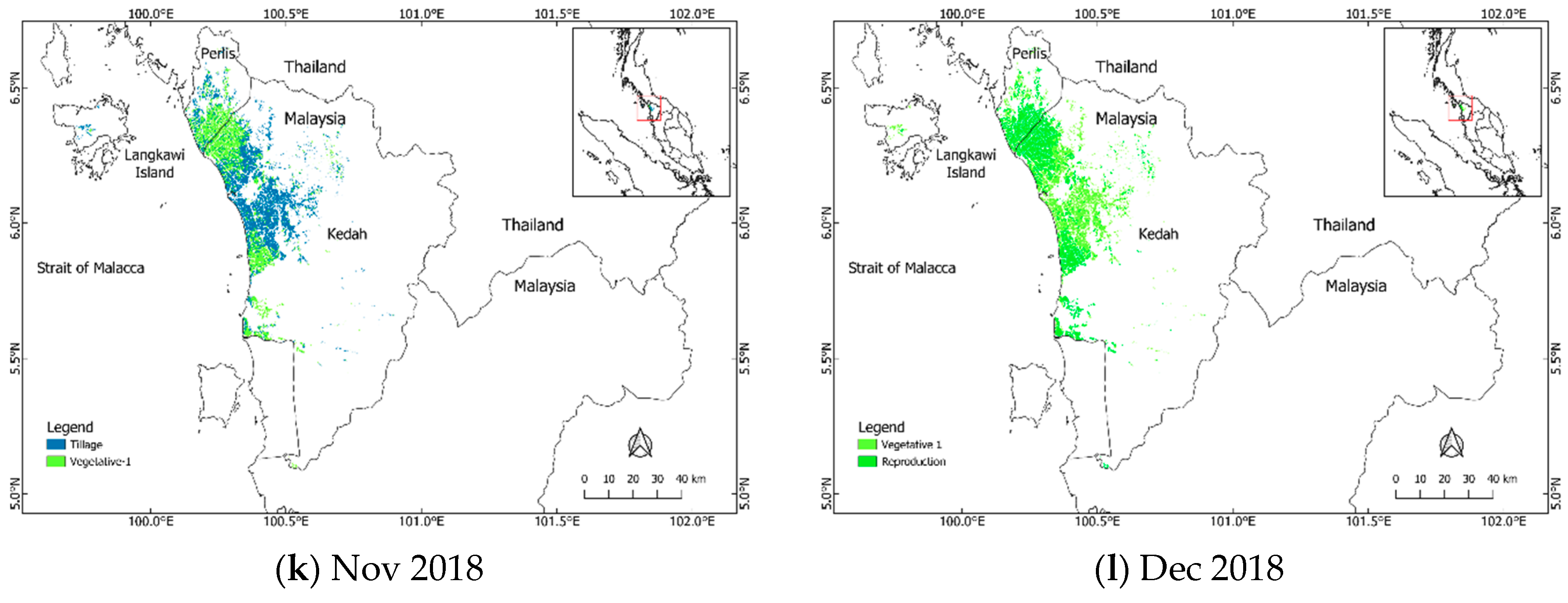
3.2. Spatiotemporal Distribution of Rice Growth Stages

Based on the analysis presented in Tables S1 and S2, Figure 9a–j (site 1) and Figure 10a–j (site 2) present the spatiotemporal distribution of rice growth stages generated from January to October 2018. At site 1, the peak land area for each stage occurred in December for tillage, January for vegetative-1, February for vegetative-2, March for reproductive stage, and April for maturity stage; which resulted in a mosaic of rice fields from three rice units: E, F and G. In the peak maturity stage, the largest harvested area was about 100,000 ha in April, and the smallest area about 10,000 ha from January to March. During the dry season, September to October, most rice fields were utilized for cash crops or left in fallow.
The rice pattern at site 2 is less complicated. Different rice growth stages peaked in terms of land area in October (tillage), November (vegetative-1), December (vegetative-2), January (reproductive), and February (maturity). These areas were mostly from rice field-X. During the off-season, crop growth stages peaked in May (tillage), June (vegetative-1), July (vegetative-2), August (reproductive), September (maturity).
Because crop growth stages are known and sequential, it is possible to forecast how much land each stage will cover. Forecasting rice field extent is important to determine appropriate food security measures related to the import and export of rice, as the trade of rice requires a supply chain and time for transportation and shipping. Figure 9k,l and Figure 10k,l predict land area for each crop stage in November and December 2018. Note these predictions are no longer valid if there is no planting, or harvest failure due to flood, drought, insect, pests and/or disease infestations. The model can only accurately forecast up to one month after maturity, as it is unknown if farmers will plant another crop.

3.3. Accuracy Assessment

Based on the VHR images from Google Earth, the predicted rice field maps (Figure 8a,b) show a high level of accuracy at the pixel level. Overall accuracy was 94.8% (site 1) and 98.2% (site 2), with a kappa coefficient of 0.89 (site 1) and 0.94 (site 2) (Table 1 and Table 2). Omission errors occurred when rice fields were classified as non-rice fields. Commission errors occurred when non-rice fields were classified as rice fields. The omission and commission errors of the rice field categories are 12.1% and 1.1% for site 1 (Table 1) and 10.2% and 5.4% for site 2 (Table 2). When the validation data from the first and second study sites were combined, the overall accuracy was 96.5%. The kappa coefficient was 0.91 (Table 3).
Figure 11 compares rice field extents derived from this study with government statistics. A high linear relationship is observed with an R2 = 0.97. From the slope of linear regression, this study underestimated rice areas by approximately 14%, which was also shown by a relatively high omission error (see Table 1, Table 2 and Table 3). Figure 11 also shows that all predicted data were consistently lower than statistical data, with RMSE = 12.73 × 1000 ha.
This study predicted that rice crops would not be planted in late September/early October, which reflects planting schedules in West Java [5]. At site 2, this study showed that rice fields in the northern and southern part of the MADA granary area are planted in October for the main season and April for the off-season. This is earlier than the central part of the MADA granary area which is planted in November for the main season and May to June for the off-season (see Section 3.1). These results are in-line with the 2016–2017 and 2017–2018 planting schedules released by the MADA granary area [59] and Department of Agriculture Peninsular Malaysia [46].

3.4. Automated Rice Cropping Pattern Mapping

Box plot results of overall accuracy and kappa coefficients for the four classification models for automated rice crop pattern mapping at the cluster level are shown in Figure 12a,b. Both SVM and ANN perform similarly, and better than random forests and C5.0. At site 1, accuracy was 83% (SVM) and 84% (ANN). Kappa coefficients were 0.73 (SVM) and 0.74 (ANN). At site 2, SVM and ANN performed better than at site 1, with the same values for overall accuracy (=1) and kappa coefficient (=1).

3.5. Comparison between Temporal VH and VV Polarization Cluster Profiles

Comparison between temporal VH and VV polarization cluster profiles for clusters of rice fields is shown in Figure S1a,b. Although both profiles for rice fields show a similar pattern, VH polarization cluster profiles for rice fields have a larger amplitude (i.e., difference between maximum and minimum peak values = around 10 dB) than the amplitude of VV polarization cluster profiles (around 7 dB). As a result, the minimum peaks at VH polarization cluster profiles for rice fields that represent soil tillage in the rice fields are developed distinctly and then increase with time sharply for about four months as a response to rice growth. Moreover, the different values of VH polarization cluster profiles at different rice growth stages are also larger than its different values in VV polarization cluster profiles.

4. Discussion

4.1. Near-Real-Time Mapping and Monitoring

Theoretically, Sentinel-1 will revisit the study area every 12 days, or six days with the two-satellite constellation (i.e., Sentinel-1A and B). The GEE team will update the data collection weekly. After a couple of days, the acquisition data from Sentinel-1 will be archived in GEE. This means that monitoring and mapping rice extent and growth stages can be conducted every 1–2 weeks. Since the algorithm has been coded in GEE and R software, the mapping processes can be done automatically. However, cluster assignment and phenological parameter extraction (during set-up phase) still require visual interpretation. The time required by GEE for clustering depends on the speed of internet access and the size of the study area. In these study areas, it took less than 20 seconds to process the data. Other processing such as cluster labelling and phenological parameter extraction take longer, about one to two hours, and depend on the number of main unit groupings.
The GEE provides Sentinel-1 data images with VV and VH dual polarization. From comparison between representative VH and VV polarization cluster profiles for clusters of rice fields in this study, it is found that the different values of VH polarization cluster profiles at different rice growth stages are more pronounced than its different values at VV polarization. It suggests that to discriminate rice growth stages, it is better to use Sentinel-1 data at VH polarization instead of VV polarization as also reported by a previous study [10].
Sentinel-1 data at VH polarization, GEE and R software are available freely in the public domain making this near-real-time mapping methodology cost-effective. Moreover, as GEE can cope with very large areas (as reported by [60], this proposed methodology can be extended to a national scale.

4.2. Establishing Time Series Datasets: Intervals and Filtering

Due to the seasonal dynamics of growth stages, time series of SAR datasets are required to detect the unique pattern of rice fields. Previous studies have used different Sentinel-1 time series intervals, ranging from 1–3 months [22], to six months or one rice season [10,21]. These short-term datasets cannot capture rice growth patterns, especially for rice fields with double crops. In this study, 26 monthly interval datasets were used, which provided enough information to detect rice growth patterns as well as forecast rice extent for two months. Datasets with numerous monthly intervals may result in too many clusters and increase data processing time. Nevertheless, this method is suitable for the long-term historical analysis of rice growth patterns.
Various researchers have attempted to establish a Sentinel-1 time series database for rice field identification. Layer stacks of time series based on acquisition date is more commonly used, such as [10,21,22]. Another approach is to use temporal metrics, including the 50th percentile and the standard deviation of VH polarization time series, and the 10th percentile of VV polarized data [19]. In this study, a median composite filter was applied to generate monthly median time series datasets. This approach was used to ensure that the whole study area was covered by Sentinel-1 data scenes and to reduce noise in the borders where data scenes overlapped. This median composite filter can also help determine trends in Sentinel-1 time series data.

4.3. Filtering Speckle Noise

Speckle noise is defined as a granular disturbance of a random nature in SAR images that leads to sudden spikes or drops in pixel-based time series [61]. Speckle noise makes it difficult to differentiate temporal features in crop growth and land cover change, such as in rice fields [19]. To reduce speckle noise in Sentinel-1 backscatter for rice mapping, spatial filtering is commonly used, such as the Gaussian [10,24], low-pass kernel [21], a spatial average for each time step of time series data [19], Gamma-MAP (Maximum A Posteriori) filter [14,16,17], the Lee filter [9,18], and averaging every 10 by 10 pixels [62]. Only three clusters at site 1 had speckle noise (Figure 5a), covering 7937 ha or 1% of the total study area. At site 2, nine clusters had speckle noise (Figure 5b) covering 119,637 ha or 14% of the area. These clusters were related to trees and built-up areas. The results suggest that processing monthly median time series of Sentinel-1 at VH polarization using a combination of K-Means, HCA and spatial median for each time step of time series data can detect and separate areas with speckle noise.

4.4. Automated Mapping

Together, supervised classification methods at the pixel level and Sentinel-1 time series data can be used to automatically map rice fields [9,10,14,22]. Another approach is the application of phenology-based decision trees at the segment level that has resulted in superpixel segmentation using the simple linear iterative clustering (SLIC) algorithm [19]. In this study, four machine learning algorithms were applied to classify the clusters that resulted from the K-means output. This approach reduced the monthly layer data from more than 75 million pixels at site 1, and 102 million pixels at site 2, to 50 clusters. It can also substantially reduce noise, which is similar to classifying the object in a superpixel segmentation approach (see [19]).
The results of the four models show that SVM and ANN were superior to the two decision tree type models: random forest and C5.0. The relatively small number of observations (50 clusters) with an imbalanced number of clusters (especially at site 2 where rice = 5 clusters vs. non-rice = 45 clusters) and the large numbers of different cluster types (especially at site 1 which had eight rice groups: Rice A, B, C, D, E, F, G and non-rice) may affect the results. Since the classification used seasonal time series data, tree models that work based on splitting the input variable are not suitable. In addition, random forests that operate to subset both observations and input variables randomly may result in biased estimates of rice or non-rice areas. SVM and ANN that are based on continuous functions are more suitable for these types of data.
Since the Sentinel-1 time series data is continuously updated, the prediction model is only valid for the same initial month and end month. For example, the model that used training data from January to December is only valid for predictions in January to December in the following year.

4.5. Comparison with Rice Extent Derived Using MODIS Data

MODIS imagery data is widely used to map rice extents [5,6,12,28,29,31,32,63,64,65,66,67,68] especially in large study areas because it has moderate resolution (250 and 500 m) and high temporal coverage. In an earlier study [5], the total rice extent at site 1, generated using MODIS data, was reported as 407,703 ha. This value is much higher than the estimated rice area in this study (302,108 ha), and higher than the field survey which estimated rice area as 351,900 ha [40]. These results suggest that the moderate resolution of MODIS data leads to overestimation of rice extent, especially in perimeter areas between non-rice and rice fields.

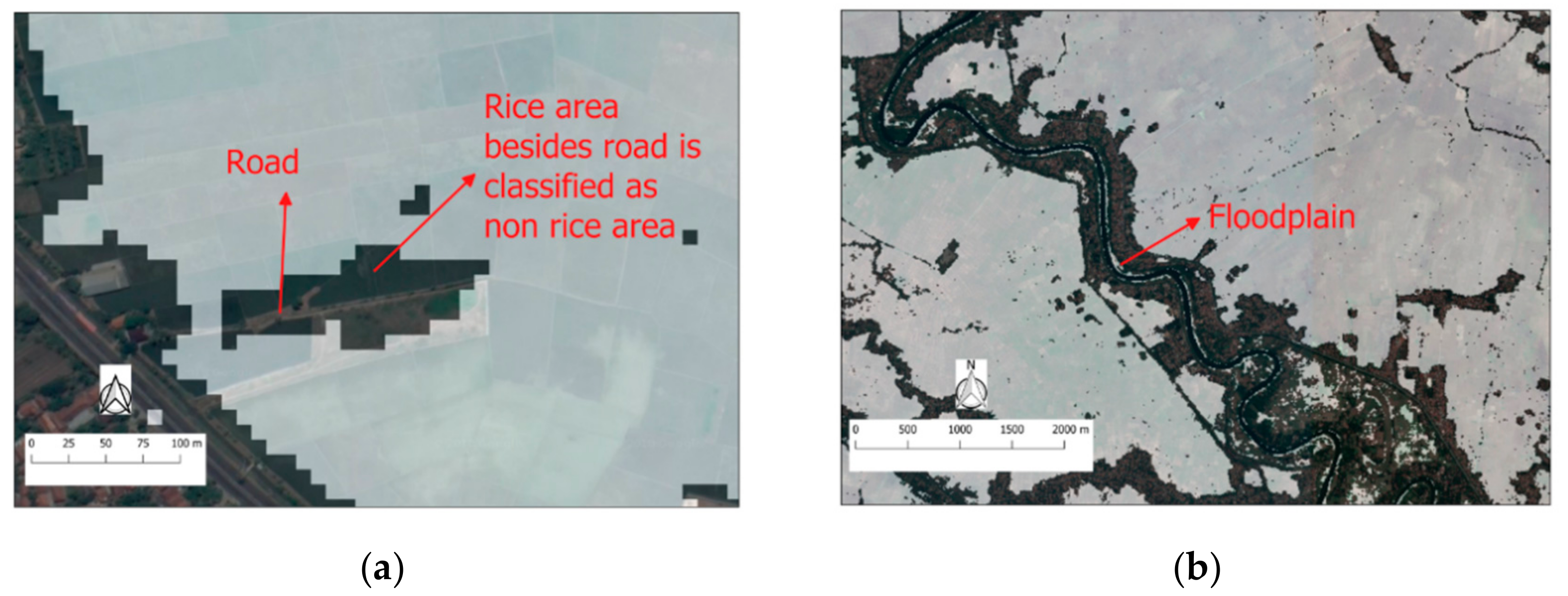
4.6. Underestimation of Rice Extent

The rice extent derived using Sentinel-1 data in this study was lower than the field survey data [39]. Similar results were reported in [10], where rice extents derived from Sentinel-1 data were lower than anticipated. This underestimation stems from the larger omission error for rice field category compared to the commission error, i.e., more rice fields were classified as non-rice fields than the opposite. Occasionally non-rice fields (usually floodplains) were classified as rice fields. Floodplains have some similarities with rice fields as the water level and soil moisture also fluctuate seasonally. These errors were usually found at the border between rice and non-rice fields (Figure 13a,b). Mixed pixel effects and the properties of the pixels in the boundaries along the field edge contributed to the error. The mixed pixel effects might be related to orbit direction as well as the angle of Sentinel-1. The mixed pixel effects have been previously reported in rice mapping and become a source of spatial uncertainty [10,19,63,66,69].

5. Conclusions

This study demonstrated that integrating Sentinel-1 data, rice phenology, and GEE cloud computing can produce automated near-real-time mapping and monitoring of rice extent, cropping patterns, and growth stages. The method is cost-effective as the Sentinel-1 data, GEE and R software are open-source and freely available. GEE has sophisticated computational infrastructure and machine learning functions that allow the proposed methodology to be computed rapidly. The resulting maps of rice growth stages and extent have a relatively high spatial resolution (10 m) and cover a large region (over 1 million ha). The data can be updated monthly.
The results show that:
  • The Indonesian rice growing area at four northern districts in West Java is 302,108 ha
  • The Malaysian rice growing area in two states, Kedah and Perlis, is 119,637 ha.
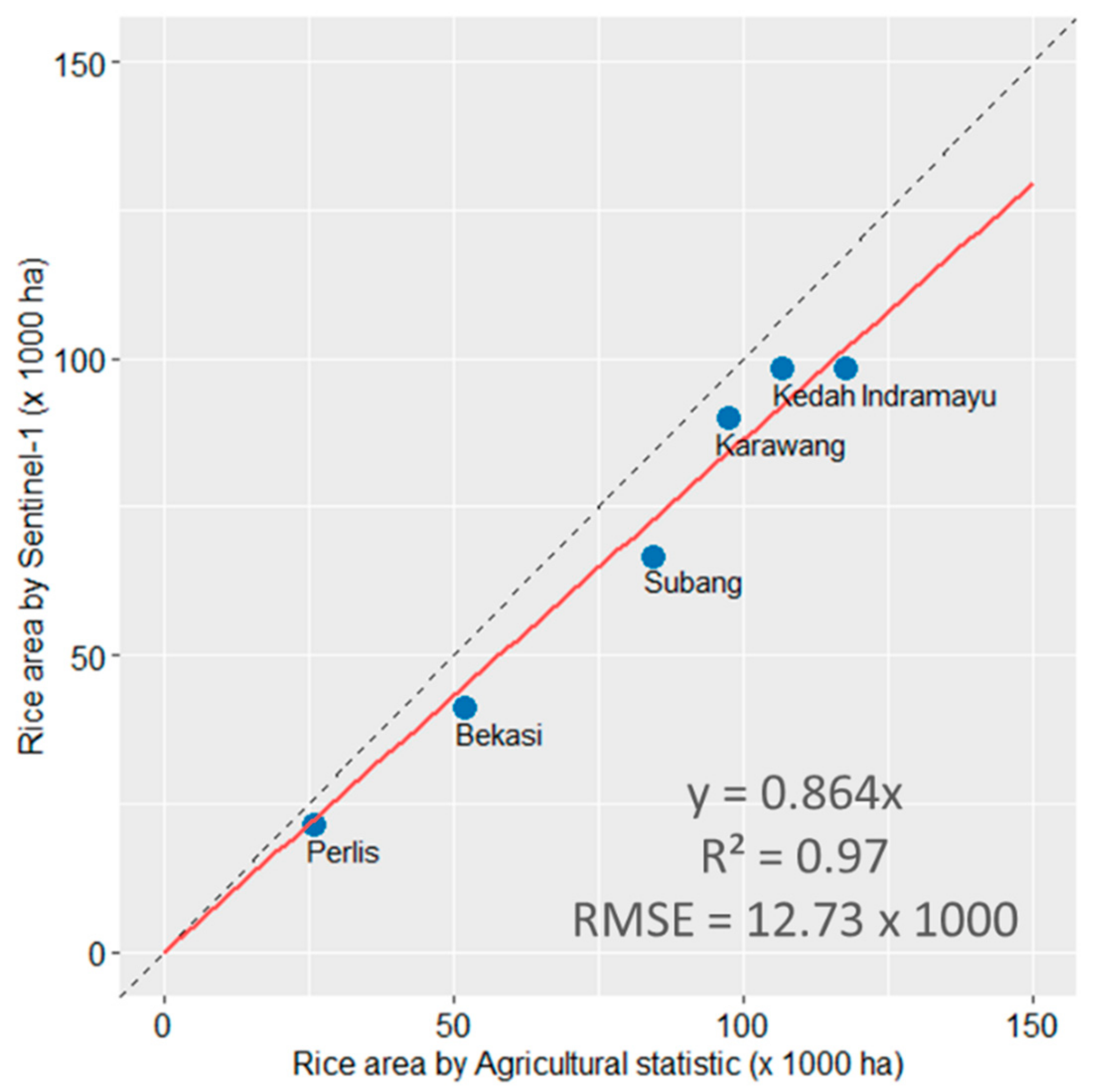
  • The overall map accuracy is 96.5% with a kappa coefficient = 0.92. Compared with government statistical data, the method underestimates rice extent by about 14%.
The approach proposed in this paper is a rapid, accurate, and cost-effective. It could be expanded to a national scale and to the whole of Southeast Asia. The Indonesian and Malaysian governments currently rely on ground sampling for data collection, which is laborious, expensive, and could be biased. The methodology in this paper could be used as an alternative source of information to field survey data. However, this approach is limited to rice extent and growth stage, and further research is necessary to estimate potential rice production of a region.

Supplementary Materials

The following are available online at https://0-www-mdpi-com.brum.beds.ac.uk/2072-4292/11/14/1666/s1, Figure S1: Comparison between representative (a) VH and (b) VV polarization cluster profiles for clusters related to rice field A, water body, built-up and tree from September 2016 to October 2018 at site 1, the northern regions of West Java, Indonesia. Table S1: Growth stages from generalized phenological parameters for rice clusters in rice fields in the northern districts of West Java, Indonesia. Table S1 corresponds to Figure 5, Figure 6, Figure 8 and Figure 9. T = Tillage, V1 = Vegetative-1, V2 = Vegetative-2, R = reproduction, M = Maturity, C = Cash crop and F (blank) = Fallow, Table S2: Growth stages from generalized phenological parameters for rice clusters in rice fields in the MADA Granary Area, Malaysia. Table S2 corresponds to Figure 5, Figure 7, Figure 8 and Figure 10. T = Tillage, V1 = Vegetative-1, V2 = Vegetative-2, R = reproduction, M = Maturity, C = Cash crop and F (blank) = Fallow.

Author Contributions

Conceptualization and research ideas, R., B.M., R.M.S., N.C.S., C.A. and B.I.S; processing the data and writing the draft paper, R.; review, editing and writing the final draft, R. and B.M.

Funding

This research received no external funding.

Acknowledgments

We thank Alisa Bryce who helped edit the manuscript.

Conflicts of Interest

The authors declare no conflict of interest.

References

  1. Kuenzer, C.; Knauer, K. Remote sensing of rice crop areas. Int. J. Remote Sens. 2013, 34, 2101–2139. [Google Scholar] [CrossRef]
  2. Sass, R.L.; Fisher, F.M., Jr.; Ding, A.; Huang, Y. Exchange of methane from rice fields: National, regional, and global budgets. J. Geophys. Res. Atmos. 1999, 104, 26943–26951. [Google Scholar] [CrossRef]
  3. Juwana, I.; Muttil, N.; Perera, B.J.C. Application of west java water sustainability index to three water catchments in west java, Indonesia. Ecol. Indic. 2016, 70, 401–408. [Google Scholar] [CrossRef]
  4. Potin, P.; Rosich, B.; Roeder, J.; Bargellini, P. Sentinel-1 Mission operations concept. In Proceedings of the 2014 IEEE Geoscience and Remote Sensing Symposium, Quebec City, QC, Canada, 13–18 July 2014; pp. 1465–1468. [Google Scholar] [CrossRef]
  5. Sianturi, R.; Jetten, V.G.; Sartohadi, J. Mapping cropping patterns in irrigated rice fields in West Java: Towards mapping vulnerability to flooding using time-series MODIS imageries. Int. J. Appl. Earth Obs. Geoinf. 2018, 66, 1–13. [Google Scholar] [CrossRef]
  6. Zhou, Y.; Xiao, X.; Qin, Y.; Dong, J.; Zhang, G.; Kou, W.; Jin, C.; Wang, J.; Li, X. Mapping paddy rice planting area in rice-wetland coexistent areas through analysis of Landsat 8 OLI and MODIS images. Int. J. Appl. Earth Obs. Geoinf. 2016, 46, 1–12. [Google Scholar] [CrossRef] [PubMed]
  7. Mosleh, M.K.; Hassan, Q.K.; Chowdhury, E.H. Application of Remote Sensors in Mapping Rice Area and Forecasting Its Production: A Review. Sensors 2015, 15, 769–791. [Google Scholar] [CrossRef] [Green Version]
  8. Phan, H.; Le Toan, T.; Bouvet, A.; Nguyen, D.L.; Pham Duy, T.; Zribi, M. Mapping of Rice Varieties and Sowing Date Using X-Band SAR Data. Sensors 2018, 18, 316. [Google Scholar] [CrossRef]
  9. Son, N.-T.; Chen, C.-F.; Chen, C.-R.; Minh, V.-Q. Assessment of Sentinel-1A data for rice crop classification using random forests and support vector machines. Geocarto Int. 2018, 33, 587–601. [Google Scholar] [CrossRef]
  10. Nguyen, D.B.; Gruber, A.; Wagner, W. Mapping rice extent and cropping scheme in the Mekong Delta using Sentinel-1A data. Remote Sens. Lett. 2016, 7, 1209–1218. [Google Scholar] [CrossRef]
  11. Lasko, K.; Vadrevu, K.P.; Tran, V.T.; Justice, C. Mapping Double and Single Crop Paddy Rice with Sentinel-1A at Varying Spatial Scales and Polarizations in Hanoi, Vietnam. IEEE J. Sel. Top. Appl. Earth Obs. Remote Sens. 2018, 11, 498–512. [Google Scholar] [CrossRef]
  12. Setiyono, D.T.; Quicho, D.E.; Gatti, L.; Campos-Taberner, M.; Busetto, L.; Collivignarelli, F.; García-Haro, J.F.; Boschetti, M.; Khan, I.N.; Holecz, F. Spatial Rice Yield Estimation Based on MODIS and Sentinel-1 SAR Data and ORYZA Crop Growth Model. Remote Sens. 2018, 10, 293. [Google Scholar] [CrossRef]
  13. Minh, V.H.; Avtar, R.; Mohan, G.; Misra, P.; Kurasaki, M. Monitoring and Mapping of Rice Cropping Pattern in Flooding Area in the Vietnamese Mekong Delta Using Sentinel-1A Data: A Case of an Giang Province. ISPRS Int. J. Geo-Inf. 2019, 8, 211. [Google Scholar] [CrossRef]
  14. Onojeghuo, A.O.; Blackburn, G.A.; Wang, Q.; Atkinson, P.M.; Kindred, D.; Miao, Y. Mapping paddy rice fields by applying machine learning algorithms to multi-temporal Sentinel-1A and Landsat data. Int. J. Remote Sens. 2018, 39, 1042–1067. [Google Scholar] [CrossRef]
  15. Tian, H.; Wu, M.; Wang, L.; Niu, Z. Mapping Early, Middle and Late Rice Extent Using Sentinel-1A and Landsat-8 Data in the Poyang Lake Plain, China. Sensors 2018, 18, 185. [Google Scholar] [CrossRef] [PubMed]
  16. Mansaray, R.L.; Huang, W.; Zhang, D.; Huang, J.; Li, J. Mapping Rice Fields in Urban Shanghai, Southeast China, Using Sentinel-1A and Landsat 8 Datasets. Remote Sens. 2017, 9, 257. [Google Scholar] [CrossRef]
  17. Mansaray, L.R.; Zhang, D.; Zhou, Z.; Huang, J. Evaluating the potential of temporal Sentinel-1A data for paddy rice discrimination at local scales. Remote Sens. Lett. 2017, 8, 967–976. [Google Scholar] [CrossRef]
  18. Yang, H.; Pan, B.; Wu, W.; Tai, J. Field-based rice classification in Wuhua county through integration of multi-temporal Sentinel-1A and Landsat-8 OLI data. Int. J. Appl. Earth Obs. Geoinf. 2018, 69, 226–236. [Google Scholar] [CrossRef]
  19. Clauss, K.; Ottinger, M.; Kuenzer, C. Mapping rice areas with Sentinel-1 time series and superpixel segmentation. Int. J. Remote Sens. 2018, 39, 1399–1420. [Google Scholar] [CrossRef]
  20. Ferrant, S.; Selles, A.; Le Page, M.; Herrault, P.-A.; Pelletier, C.; Al-Bitar, A.; Mermoz, S.; Gascoin, S.; Bouvet, A.; Saqalli, M.; et al. Detection of Irrigated Crops from Sentinel-1 and Sentinel-2 Data to Estimate Seasonal Groundwater Use in South India. Remote Sens. 2017, 9, 1119. [Google Scholar] [CrossRef]
  21. Mandal, D.; Kumar, V.; Bhattacharya, A.; Rao, Y.S.; Siqueira, P.; Bera, S. Sen4Rice: A Processing Chain for Differentiating Early and Late Transplanted Rice Using Time-Series Sentinel-1 SAR Data with Google Earth Engine. IEEE Geosci. Remote Sens. Lett. 2018, 15, 1947–1951. [Google Scholar] [CrossRef]
  22. Mohite, J.D.; Sawant, S.A.; Kumar, A.; Prajapati, M.; Pusapati, S.V.; Singh, D.; Pappula, S. Operational Near Real Time Rice Area Mapping Using Multi-Temporal Sentinel-1 SAR Observations. Int. Arch. Photogramm. Remote Sens. Spat. Inf. Sci. 2018, XLII–4, 433–438. [Google Scholar] [CrossRef]
  23. Setiyono, T.D.; Quicho, E.D.; Holecz, F.H.; Khan, N.I.; Romuga, G.; Maunahan, A.; Garcia, C.; Rala, A.; Raviz, J.; Collivignarelli, F.; et al. Rice yield estimation using synthetic aperture radar (SAR) and the ORYZA crop growth model: Development and application of the system in South and South-east Asian countries AU - Setiyono, T.D. Int. J. Remote Sens. 2018, 1–32. [Google Scholar] [CrossRef]
  24. Nguyen, D.B.; Wagner, W. European Rice Cropland Mapping with Sentinel-1 Data: The Mediterranean Region Case Study. Water 2017, 9, 392. [Google Scholar] [CrossRef]
  25. Fikriyah, V.N.; Darvishzadeh, R.; Laborte, A.; Khan, N.I.; Nelson, A. Discriminating transplanted and direct seeded rice using Sentinel-1 intensity data. Int. J. Appl. Earth Obs. Geoinf. 2019, 76, 143–153. [Google Scholar] [CrossRef]
  26. Torbick, N.; Chowdhury, D.; Salas, W.; Qi, J. Monitoring Rice Agriculture across Myanmar Using Time Series Sentinel-1 Assisted by Landsat-8 and PALSAR-2. Remote Sens. 2017, 9, 119. [Google Scholar] [CrossRef]
  27. Dong, J.; Xiao, X. Evolution of regional to global paddy rice mapping methods: A review. ISPRS J. Photogramm. Remote Sens. 2016, 119, 214–227. [Google Scholar] [CrossRef] [Green Version]
  28. Sakamoto, T.; Van Nguyen, N.; Ohno, H.; Ishitsuka, N.; Yokozawa, M. Spatio–temporal distribution of rice phenology and cropping systems in the Mekong Delta with special reference to the seasonal water flow of the Mekong and Bassac rivers. Remote Sens. Env. 2006, 100, 1–16. [Google Scholar] [CrossRef]
  29. Gumma, M.K.; Thenkabail, P.S.; Teluguntla, P.; Rao, M.N.; Mohammed, I.A.; Whitbread, A.M. Mapping rice-fallow cropland areas for short-season grain legumes intensification in South Asia using MODIS 250 m time-series data. Int. J. Digit. Earth 2016, 9, 981–1003. [Google Scholar] [CrossRef] [Green Version]
  30. Nguyen, T.T.H.; De Bie, C.A.J.M.; Ali, A.; Smaling, E.M.A.; Chu, T.H. Mapping the irrigated rice cropping patterns of the Mekong delta, Vietnam, through hyper-temporal SPOT NDVI image analysis. Int. J. Remote Sens. 2012, 33, 415–434. [Google Scholar] [CrossRef]
  31. Asilo, S.; De Bie, K.; Skidmore, A.; Nelson, A.; Barbieri, M.; Maunahan, A. Complementarity of Two Rice Mapping Approaches: Characterizing Strata Mapped by Hypertemporal MODIS and Rice Paddy Identification Using Multitemporal SAR. Remote Sens. 2014, 6, 12789–12814. [Google Scholar] [CrossRef] [Green Version]
  32. Mosleh, K.M.; Hassan, K.Q. Development of a Remote Sensing-Based “Boro” Rice Mapping System. Remote Sens. 2014, 6, 1938–1953. [Google Scholar] [CrossRef]
  33. Manjunath, K.R.; More, R.S.; Jain, N.K.; Panigrahy, S.; Parihar, J.S. Mapping of rice-cropping pattern and cultural type using remote-sensing and ancillary data: A case study for South and Southeast Asian countries. Int. J. Remote Sens. 2015, 36, 6008–6030. [Google Scholar] [CrossRef]
  34. Ali, A.; de Bie, C.A.J.M.; Skidmore, A.K.; Scarrott, R.G.; Hamad, A.; Venus, V.; Lymberakis, P. Mapping land cover gradients through analysis of hyper-temporal NDVI imagery. Int. J. Appl. Earth Obs. Geoinf. 2013, 23, 301–312. [Google Scholar] [CrossRef]
  35. Mansaray, L.R.; Wang, F.; Huang, J.; Yang, L.; Kanu, A.S. Accuracies of support vector machine and random forest in rice mapping with Sentinel-1A, Landsat-8 and Sentinel-2A datasets. Geocarto Int. 2019, 1–21. [Google Scholar] [CrossRef]
  36. Gorelick, N.; Hancher, M.; Dixon, M.; Ilyushchenko, S.; Thau, D.; Moore, R. Google Earth Engine: Planetary-scale geospatial analysis for everyone. Remote Sens. Env. 2017, 202, 18–27. [Google Scholar] [CrossRef]
  37. Padarian, J.; Minasny, B.; McBratney, A.B. Using Google’s cloud-based platform for digital soil mapping. Comput. Geosci. 2015, 83, 80–88. [Google Scholar] [CrossRef]
  38. Hansen, M.C.; Potapov, P.V.; Moore, R.; Hancher, M.; Turubanova, S.A.; Tyukavina, A.; Thau, D.; Stehman, S.V.; Goetz, S.J.; Loveland, T.R.; et al. High-resolution global maps of 21st-century forest cover change. Science 2013, 342, 850–853. [Google Scholar] [CrossRef]
  39. Panuju, D.R.; Mizuno, K.; Trisasongko, B.H. The dynamics of rice production in Indonesia 1961–2009. J. Saudi Soc. Agric. Sci. 2013, 12, 27–37. [Google Scholar] [CrossRef]
  40. Pusat Data dan Analisa Pembangunan Jawa Barat. Available online: http://pusdalisbang.jabarprov.go.id/pusdalisbang/data-49-pertanian.html (accessed on 25 June 2019).
  41. Yanto; Rajagopalan, B.; Zagona, E. Space–time variability of Indonesian rainfall at inter-annual and multi-decadal time scales. Clim. Dyn. 2016, 47, 2975–2989. [Google Scholar] [CrossRef]
  42. Nasution, C.; Syaifullah, D. Analisis spasial indeks kekeringan daerah pantai utara (Pantura) Jawa Barat. J. Air Indones. 2005, 1, 235–243. [Google Scholar]
  43. De Dapper, J.; Debaveye, M. Geomorphology and soils of the Padang Terap District, Kedah, Peninsular Malaysia. Bul. Persat. Geol. Malays. Bull. Geol. Soc. Malays. 1986, 20, 765–790. [Google Scholar] [Green Version]
  44. Othman, M.; Ash’aari, Z.H.; Muharam, F.M.; Sulaiman, W.N.A.; Hamisan, H.; Mohamad, N.D.; Othman, N.H. Assessment of drought impacts on vegetation health: A case study in Kedah. IOP Conf. Ser. Earth Env. Sci. 2016, 37, 12072. [Google Scholar] [CrossRef]
  45. Tan, K.C. Rainfall Patterns Analysis over Ampangan Muda, Kedah from 2007–2016. J. Phys. Conf. Ser. 2018, 995, 12121. [Google Scholar] [CrossRef]
  46. Department of Agriculture Peninsular Malaysia. Paddy Statistics of Malaysia 2015; Department of Agriculture Peninsular Malaysia: Kuching, Malaysia, 2016. [Google Scholar]
  47. Nelson, A.; Setiyono, T.; Rala, B.A.; Quicho, D.E.; Raviz, V.J.; Abonete, J.P.; Maunahan, A.A.; Garcia, A.C.; Bhatti, Z.H.; Villano, S.L.; et al. Towards an Operational SAR-Based Rice Monitoring System in Asia: Examples from 13 Demonstration Sites across Asia in the RIICE Project. Remote Sens. 2014, 6, 10773–10812. [Google Scholar] [CrossRef] [Green Version]
  48. Nazuri, N.S.; Man, N. Acceptance and Practices on New Paddy Seed Variety Among Farmers in MADA Granary Area. Acad. J. Interdiscip. Stud. 2016, 5. [Google Scholar] [CrossRef] [Green Version]
  49. Muda Agriculture Development Authority (MADA). Available online: http://www.mada.gov.my/?page_id=13023&lang=en (accessed on 25 June 2019).
  50. What are the technical specifications for Google Imagery? Available online: https://support.google.com/mapsdata/answer/6261838?hl=en&ref_topic=6250082 (accessed on 25 June 2019).
  51. De Bie, C.A.J.M.; Nguyen, T.T.H.; Ali, A.; Scarrott, R.; Skidmore, A.K. LaHMa: A landscape heterogeneity mapping method using hyper-temporal datasets. Int. J. Geogr. Inf. Sci. 2012, 26, 2177–2192. [Google Scholar] [CrossRef]
  52. R Development Core Team. R: A Language and Environment for Statistical Computing. R Foundation for Statistical Computing: Vienna, Austria, 2016. Available online: http://www.R-project.org/ (accessed on 2 January 2019).
  53. Karatzoglou, A.; Smola, A.; Hornik, K.; Zeileis, A. Kernlab—An S4 Package for Kernel Methods in R. J. Stat. Softw. 2004, 1. [Google Scholar] [CrossRef]
  54. Venables, W.N.; Ripley, B.D. Modern Applied Statistics with S, 4th ed.; Springer Publishing Company: New York, NY, USA, 2002; ISBN 0387954570. [Google Scholar]
  55. Liaw, A.; Wiener, M. Package ‘randomForest’. Breiman and Cutler’s random forests for classification and regression. CRAN Ref. Man. 2014, 4, 6–10. [Google Scholar]
  56. Quinlan, R. C4.5: Programs for Machine Learning; Morgan Kaufmann Publishers: Burlington, MA, USA, 1993. [Google Scholar]
  57. Kuhn, M.; Weston, S.; Culp, M.; Coulter, N.; Quinlan, R. C50: C5.0 Decision Trees and Rule-Based Models; R Development Core Team: Vienna, Austria, 2018. [Google Scholar]
  58. Kuhn, M.; Wing, J.; Weston, S.; Williams, A.; Keefer, C.; Engelhardt, A. Caret: Classification and Regression Training. Available online: https://Cran.R-Project.Org/Package=Caret (accessed on 27 March 2019).
  59. Halaman web rasmi Lembaga Kemajuan Pertanian Muda (MADA). Available online: http://www.mada.gov.my/?page_id=1715 (accessed on 30 June 2019).
  60. Dong, J.; Xiao, X.; Menarguez, M.A.; Zhang, G.; Qin, Y.; Thau, D.; Biradar, C.; Moore, B. Mapping paddy rice planting area in northeastern Asia with Landsat 8 images, phenology-based algorithm and Google Earth Engine. Remote Sens. Env. 2016, 185, 142–154. [Google Scholar] [CrossRef] [Green Version]
  61. Argenti, F.; Lapini, A.; Bianchi, T.; Alparone, L. A Tutorial on Speckle Reduction in Synthetic Aperture Radar Images. IEEE Geosci. Remote Sens. Mag. 2013, 1, 6–35. [Google Scholar] [CrossRef] [Green Version]
  62. Gao, Q.; Zribi, M.; Escorihuela, J.M.; Baghdadi, N.; Segui, Q.P. Irrigation Mapping Using Sentinel-1 Time Series at Field Scale. Remote Sens. 2018, 10, 1495. [Google Scholar] [CrossRef]
  63. Xiao, X.; Boles, S.; Frolking, S.; Li, C.; Babu, J.Y.; Salas, W.; Moore, B. Mapping paddy rice agriculture in South and Southeast Asia using multi-temporal MODIS images. Remote Sens. Env. 2006, 100, 95–113. [Google Scholar] [CrossRef]
  64. Zhang, G.; Xiao, X.; Dong, J.; Kou, W.; Jin, C.; Qin, Y.; Zhou, Y.; Wang, J.; Menarguez, M.A.; Biradar, C. Mapping paddy rice planting areas through time series analysis of MODIS land surface temperature and vegetation index data. ISPRS J. Photogramm. Remote Sens. 2015, 106, 157–171. [Google Scholar] [CrossRef] [PubMed] [Green Version]
  65. Tornos, L.; Huesca, M.; Dominguez, J.A.; Moyano, M.C.; Cicuendez, V.; Recuero, L.; Palacios-Orueta, A. Assessment of MODIS spectral indices for determining rice paddy agricultural practices and hydroperiod. ISPRS J. Photogramm. Remote Sens. 2015, 101, 110–124. [Google Scholar] [CrossRef] [Green Version]
  66. Clauss, K.; Yan, H.; Kuenzer, C. Mapping Paddy Rice in China in 2002, 2005, 2010 and 2014 with MODIS Time Series. Remote Sens. 2016, 8, 434. [Google Scholar] [CrossRef]
  67. Qin, Y.; Xiao, X.; Dong, J.; Zhou, Y.; Zhu, Z.; Zhang, G.; Du, G.; Jin, C.; Kou, W.; Wang, J.; et al. Mapping paddy rice planting area in cold temperate climate region through analysis of time series Landsat 8 (OLI), Landsat 7 (ETM+) and MODIS imagery. ISPRS J. Photogramm. Remote Sens. 2015, 105, 220–233. [Google Scholar] [CrossRef] [Green Version]
  68. Setiawan, Y.; Rustiadi, E.; Yoshino, K.; Liyantono; Effendi, H. Assessing the Seasonal Dynamics of the Java’s Paddy Field Using MODIS Satellite Images. ISPRS Int. J. Geo-Inf. 2014, 3, 110–129. [Google Scholar] [CrossRef]
  69. Singha, M.; Dong, J.; Zhang, G.; Xiao, X. High resolution paddy rice maps in cloud-prone Bangladesh and Northeast India using Sentinel-1 data. Sci. Data 2019, 6, 26. [Google Scholar] [CrossRef]
Figure 1. Map of study area comprises four districts at the northern region of West Java, Indonesia and two states: Kedah and Perlis in Malaysia. Coverage of the used ascending and descending modes of Sentinel-1A scenes is shown by red and blue shades, respectively. Source of the background map: Google Maps.
Remotesensing 11 01666 g001
Figure 2. Workflow of mapping and monitoring rice cropping patterns, growth stages and extent using Sentinel-1 time series data on the Google Earth Engine platform.
Remotesensing 11 01666 g002
Figure 3. (a) Time series of Sentinel-1 backscatter at VH polarization in the field router location. WPS: wet planting season. DPS: dry planting season. F-CC: fallow and or cash crops. (b) Ground survey photos of rice field taken by the field router. Note that photos for April 2017, and February and March 2018 are not available. Labels in these months are based on preceding and proceeding growth stages in May 2017 and Jan 2018.
Remotesensing 11 01666 g003
Figure 4. Time series of Sentinel-1 backscatter at VH polarization for four land-cover classes: rice field, water body, tree and built-up.
Remotesensing 11 01666 g004
Figure 5. Dendrogram resulting from the hierarchical clustering analysis (HCA) of representative VH polarization clusters profiles in Figure 6 and Figure 7 for (a) the northern districts of West Java, Indonesia represented and (b) Kedah and Perlis states, Malaysia, respectively.
Remotesensing 11 01666 g005
Figure 6. Representative VH polarization cluster profiles for clusters related to rice field, water body, built-up and tree from September 2016 to October 2018 at the first study area, the northern regions of West Java, Indonesia. Seven rice field classes were obtained: ((a)–(g) are for rice field A, B, C, D, E, F and G) using the hierarchical clustering analysis (HCA) as shown in Figure 5a.
Remotesensing 11 01666 g006
Figure 7. Representative VH polarization cluster profiles for clusters related to rice field, water body, built-up and tree from September 2016 to October 2018 at the second study area, Kedah and Perlis states, Malaysia. Two rice field groups were obtained ((a) and (b) are for rice field X and Y) using the hierarchical clustering analysis (HCA) as shown in Figure 5b.
Remotesensing 11 01666 g007
Figure 8. Spatial distribution of rice field cropping patterns in (a) the northern districts of West Java, Indonesia represented as 7 rice units and (b) Kedah and Perlis states, Malaysia represented as 2 rice units. Figure 8a corresponds to Figure 5a and Figure 6 and Table S1. Figure 8b corresponds to Figure 5b and Figure 7 and Table S2.
Remotesensing 11 01666 g008
Figure 9. Rice growth varies in space and time at the northern districts of West Java, Indonesia. Figure 9 corresponds to Table S1.
Remotesensing 11 01666 g009aRemotesensing 11 01666 g009b
Figure 10. Rice growth varies in space and time at Kedah and Perlis states, Malaysia. Figure 10 corresponds to Table S2.
Remotesensing 11 01666 g010aRemotesensing 11 01666 g010bRemotesensing 11 01666 g010c
Figure 11. Comparison between the estimated and observed areas of rice fields derived Figure 1 and statistical data at district and states levels for the first and second study areas, respectively. The two solid lines represent the linear regression with zero intercept between the two datasets. The dash line is the identity line—x = y line.
Remotesensing 11 01666 g011
Figure 12. Accuracy and Kappa for four supervised models in classifying clusters based on its labels (a) at the northern districts of West Java, Indonesia and (b) Kedah and Perlis states, Malaysia.
Remotesensing 11 01666 g012
Figure 13. Sources of error in rice field classification using Sentinel-1 backscatter in VH polarization. White colour is a region that classified as rice fields, while RGB colour is for non-rice fields. Location coordinates of (a) and (b) are 108.472603°E, 6.494271°S and 107.16626°E, 6.08264°S, respectively.
Remotesensing 11 01666 g013
Table 1. Confusion matrix for the rice classification at the Northern Region of West Java Indonesia.
Predicted Class Producer Accuracy
Non-Rice (Pixels)Rice
(Pixels)
Total
(Pixels)
Percent CorrectOmission Error (%)
Reference classNon-rice
(pixels)
299230199.30.7
Rice
(pixels)
2417519987.912.1
Total
(pixels)
323177500
Users accuracy
Percent correct92.698.9 94.80
Commission error (%)7.41.1
Kappa0.89
Table 2. Confusion matrix for the rice classification at the Kedah and Perlis states, Malaysia.
Predicted Class Producer Accuracy
Non-rice (Pixels)Rice
(Pixels)
Total
(Pixels)
Percent CorrectOmission Error (%)
Reference classNon-rice
(pixels)
438344199.30.7
Rice
(pixels)
6535989.810.2
Total
(pixels)
44456500
Users accuracy
Percent correct98.694.6 98.20
Commission error (%)1.45.4
Kappa0.94
Table 3. Confusion matrix for the rice classification at combination of both study sites.
Predicted Class Producer Accuracy
Non-rice (Pixels)Rice
(Pixels)
Total
(Pixels)
Percent CorrectOmission Error (%)
Reference classNon-rice
(pixels)
737574299.30.7
Rice
(pixels)
3022825888.411.6
Total
(pixels)
7672331000
Users accuracy
Percent correct96.197.9 96.50
Commission error (%)3.92.1
Kappa0.91

