Thermal Airborne Optical Sectioning


Institute of Computer Graphics, Johannes Kepler University Linz, 4040 Linz, Austria
*
Author to whom correspondence should be addressed.
Remote Sens. 2019, 11(14), 1668; https://0-doi-org.brum.beds.ac.uk/10.3390/rs11141668
Submission received: 4 June 2019
/
Revised: 26 June 2019
/
Accepted: 12 July 2019
/
Published: 13 July 2019
(This article belongs to the Special Issue Multispectral Image Acquisition, Processing and Analysis)
Abstract
:We apply a multi-spectral (RGB and thermal) camera drone for synthetic aperture imaging to computationally remove occluding vegetation for revealing hidden objects, as required in archeology, search-and-rescue, animal inspection, and border control applications. The radiated heat signal of strongly occluded targets, such as a human bodies hidden in dense shrub, can be made visible by integrating multiple thermal recordings from slightly different perspectives, while being entirely invisible in RGB recordings or unidentifiable in single thermal images. We collect bits of heat radiation through the occluder volume over a wide synthetic aperture range and computationally combine them to a clear image. This requires precise estimation of the drone’s position and orientation for each capturing pose, which is supported by applying computer vision algorithms on the high resolution RGB images.
1. Introduction
Synthetic apertures (SA) find applications in many fields, such as radar [1,2,3], radio telescopes [4,5], microscopy [6], sonar [7,8], ultrasound [9,10], LiDAR [11,12], and optical imaging [13,14,15,16,17,18,19,20]. They approximate the signal of a single hypothetical wide aperture sensor with either an array of static small-aperture sensors or a single-moving small aperture sensor whose individual signals are computationally combined to increase resolution, depth-of-field, frame rate, contrast, and signal-to-noise ratio.
With airborne optical sectioning (AOS) [21,22], we apply camera drones for synthetic aperture imaging. They sample the optical signal of wide synthetic apertures (up to 100 m diameter) with multiscopic video images as an unstructured (irregularly sampled) light field to support optical slicing by image integration. By computationally removing occluding vegetation or trees when inspecting the ground surface, AOS supports various applications in archaeology, forestry, and agriculture.
In [23] we derive a statistical model that reveals practical limits to both synthetic aperture size and number of samples for the application of occlusion removal. This leads to an understanding on how to design synthetic aperture sampling patterns and sensors in a most optimal and practically efficient way. For AOS recordings, we achieve an approximately 6.5–12.75 times reduction of the synthetic aperture area and an approximately 10–20 times lower number of samples without significant loss in visibility.
Compared to alternative airborne scanning technologies (such as LiDAR), AOS is cheaper, delivers surface color information, achieves higher sampling resolutions, and (in contrast to photogrammetry) it does not suffer from inaccurate correspondence matches and long processing times. Rather than to measure, compute, and render 3D point clouds or triangulated 3D meshes, AOS applies image-based rendering for 3D visualization. However, AOS, like photogrammetry, is passive (it only receives reflected light and does not emit electromagnetic or sound waves to measure the backscattered signal). Thus, it relies on an external energy source (i.e., sunlight).
While thermal scanning with robot arms has been recently demonstrated under short-range and controlled laboratory conditions [24], in this article we present first results of AOS being applied to thermal imaging in outdoor environments. The radiated heat signal of strongly occluded targets, such as human bodies hidden in dense shrub, can be made visible by integrating multiple thermal recordings from slightly different perspectives, while being entirely invisible in RGB recordings or unidentifiable in single thermal images. We refer to the extension of AOS to thermal imaging as thermal airborne optical sectioning (TAOS). In contrast to AOS, TAOS does not rely on the reflectance of sunlight from the target, which is low in case of dense occlusion. Instead, it collects bits of heat radiation through the occluder volume over a wide synthetic aperture range and computationally combines them to a clear image. This process requires precise estimation of the drone’s position and orientation for each capturing pose. Since GPS, internal inertia sensors, and compass modules or pose estimation from low resolution thermal images [25] are too imprecise, and light-weight thermal cameras have too-low resolutions, an additional high-resolution RGB camera is used to support accurate pose estimation based on computer vision. TAOS might find applications in areas where classical airborne thermal imaging is already used, such as search-and-rescue, animal inspection, forestry, agriculture, or border control. It enables the penetration of densely occluding vegetation.
2. Results
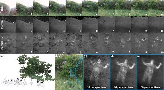
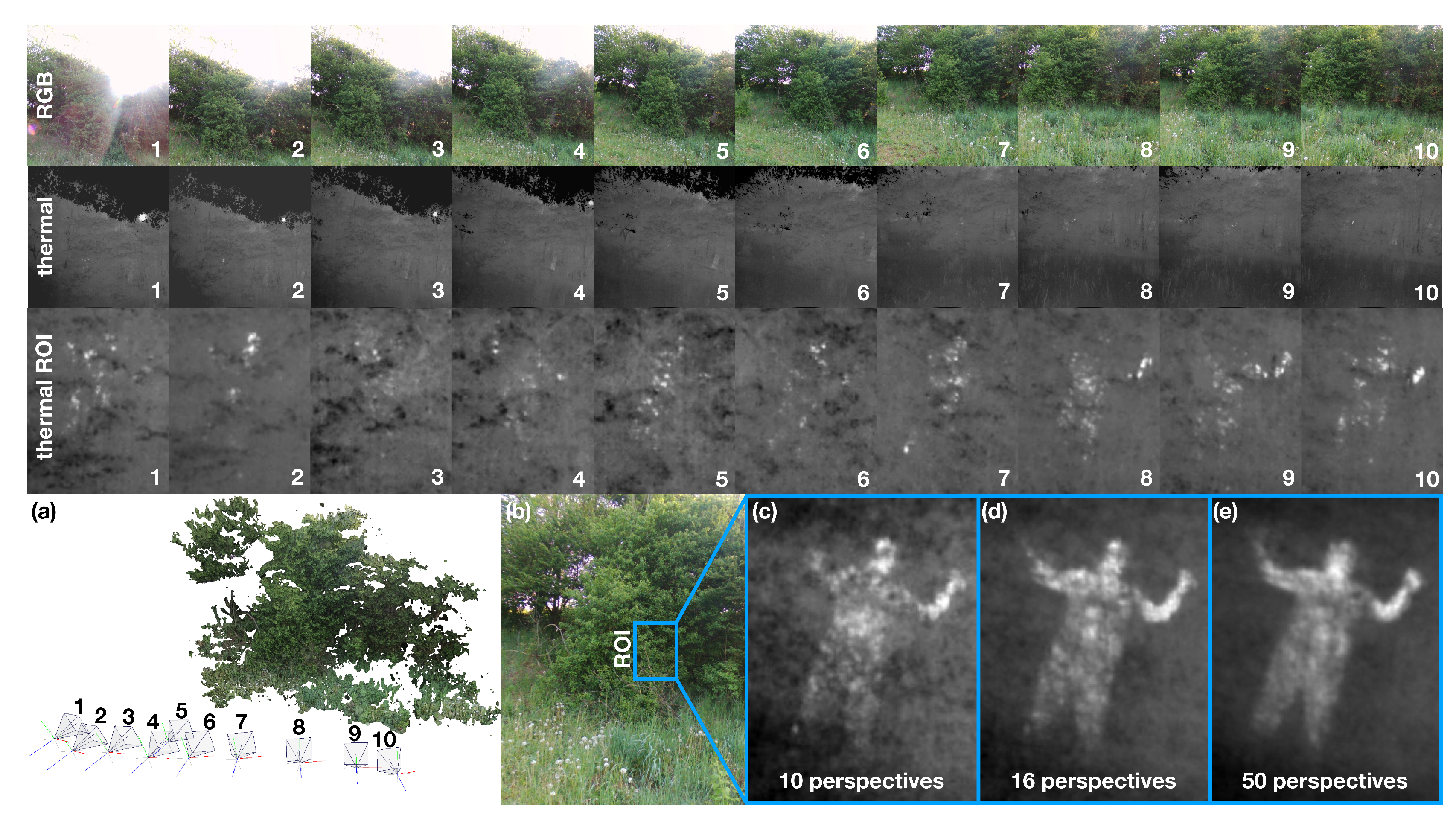
Figure 1 illustrates the results of a first field experiment. Our camera drone captures a series of 10 pairs of RGB images (first row) and thermal images (second row) of a dense bush along a horizontal path (Figure 1a). The approximate distance between each pose of 0.8 m leads to a linear synthetic aperture of 7.2 m. The distance to the bush was approximately 6.7 m. Neither in the RGB images nor in the thermal images is our target (a person hiding behind the bush) visible. The third row shows close-ups of the region of interest (ROI, Figure 1b) in which the target is located. While each thermal image carries bits of the target’s heat signal, it cannot be identified without knowing it in advance. The high-resolution ( pixels) RGB images are processed using a state of the art structure-from-motion and multi-view stereo pipeline [26] and the result is used for pose estimation only (Figure 1a). The pose estimation error in this experiment was 0.36 pixels (on the RGB camera’s image sensor). This is the average mis-registration (due to imprecise pose estimation) between scene features when back-projecting them to all 10 RGB images and comparing these back-projections to their corresponding image features. Since RGB camera and thermal camera have a fixed relative alignment on the drone and a similar field of view, the pose estimation error can be directly scaled to the lower resolution ( ) of the thermal camera. Due to the larger pixels, the average pose estimation error was 0.18 pixels on the sensor of the thermal camera. Thus, 0.18 pixels is the average misalignment between the 10 thermal images when they are computationally integrated for AOS. Considering an approximate distance of 11 m to our target, the spatial sampling resolution of TAOS in this experiment was 1408 pixels m−2 (considering the size of thermal pixels, the uncertainty due to errors in pose estimation [21], and the distance to the target).
By computationally integrating all 10 registered thermal images, the target becomes clearly visible (Figure 1c). The reason for this is, that pixels on surface points of the target perfectly align (up to the error caused by pose estimation) in focussed points while occluders in front of the target misalign and result in defocussed points. This is the core principle of AOS: sampling a wide SA signal to profit from a shallow depth-of-field that quickly blurs out-of-focus occluders to reveal focussed targets. However, since the distance to the target is unknown, we must computationally sweep a synthetic focal plane through all depth layers until the target becomes visible. This is what is commonly done in optical sectioning for microscopy. Section 4 will briefly summarize the AOS image integration process. Since an in-depth discussion is out of scope for this article, more details on the image-based rendering process can be found in [21].
Figure 1d,e illustrates that the results can be improved by capturing and combining more samples (up to 50) over a wider synthetic aperture. However, we have previously shown that there exist limits on the synthetic aperture size and number of samples which depend on the average projected size and disparity of occluders on the image sensor [23]. Relatively small apertures with a relatively low number of samples already lead to optimal results, while larger apertures and additional samples do not provide improvements. Figure 1c–e underlines these findings, as there is only a slight improvement between 10 samples and 16 samples, but no significant improvement when the number of samples is increased to 50. Figure 1e does not show additional unoccluded features on the target, but only a stronger blur that results from more (slightly misaligned) images being integrated. More details on the statistical theory of SA sampling can be found in [23].
3. Discussion
TAOS has the potential to increase depth penetration through densely occluding vegetation for airborne thermal imaging applications. For many such applications that inspect moving targets (such as search-and-rescue, animal inspection, or border control), fast update rates are required.
Compared to direct thermal imaging, TAOS introduces an additional processing overhead for image rectification, pose estimation, and image integration. However, for each new pose, only one new image is added to the integral while the oldest is removed from the integral. Therefore, the overhead is restricted to processing a single image only, rather than processing all N images that are integrated. In our experiments, image processing was done offline (after recording) and was not performance optimized. We timed approximately 8.5 s for all N = 10 images together (i.e., on average 850 ms per image). Real-time pose estimation [27], image rectification [28], and rendering techniques [29] will reduce this overhead at least to 107 ms per image. Thus, if direct thermal imaging delivers recordings at 10 fps, TAOS (for N = 10) would deliver at approximately 7 fps for pixels—causing a slightly larger pose estimation error (0.49 pixels on the sensor of the thermal camera). However, TAOS images integrate a history of N frames. For our example above, this means that, while direct thermal imaging integrates over 100 ms (1 frame), TAOS integrates over 1 s (N = 10 frames). Faster cameras and processors will improve performance. Moving targets will result in motion blur that can lead to objects being undetectable during TAOS integration (depending on the object’s size and position in the scene). TAOS can compensate for known object motion, so that moving objects can be focused during integration. Furthermore, we currently rely on a mainly static scene for pose estimation. If major parts of the scene are moving or changing during one TAOS recording (e.g., 10 frames) the pose estimation will be imprecise and integration might fail.
Another limitation is that, currently, since pose estimation relies on features in high-resolution RGB images, TAOS cannot be applied in low-light conditions (e.g., at night) unless the spatial and tonal resolutions of thermal cameras increase, or a precise non-image-based pose estimation method, such as Real Time Kinematic GPS, is applied. Our initial experiments on pose estimation with the thermal images did not lead to a useful precision.
4. Materials and Methods
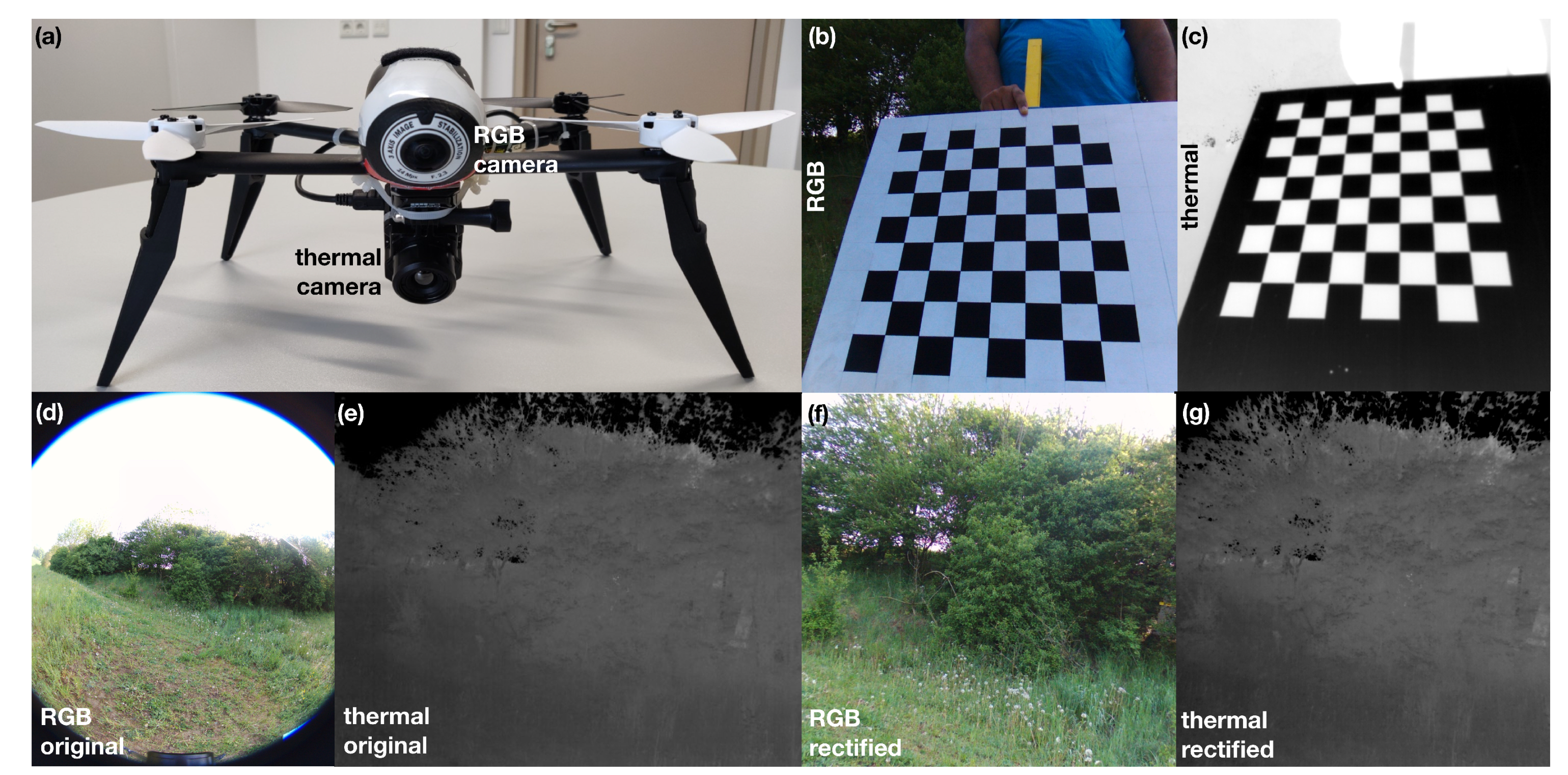
The drone used for our experiment (Figure 2a) was a Parrot Bebop 2 (Parrot Drones SAS, Paris, France) with an internal RGB camera (14 MP CMOS sensor, fixed 178 FOV fisheye lens, 8 bit per color channel). Note that we rectify and crop the original image and downscale the resolution to pixels for performance reasons. We attached an external thermal camera at the drone’s vertical gravity axis (a FLIR Vue Pro; FLIR Systems, Inc. Wilsonville, Oregon, USA; pixels rectified and cropped to pixels; fixed 81 FOV lens; 14 bit for a 7.5–13.5 spectral band). Note that both cameras are rectified to the same field of view of 53 .
For image rectification (Figure 2d–g), lens distortion of both cameras has to be determined and corrected. Furthermore, we calibrate the relative offset between the two camera positions with an affine transformation (containing rotation and translation in 3D). Thus, absolute camera positions of the RGB images can be transformed to the thermal recordings. To support rectification and calibration, we used a metal plate with glued black velvet squares aligned in a checker board pattern. While the color difference is only visible in the RGB camera (Figure 2b), the thermal difference between the metal and the velvet is detectable in the thermal camera (Figure 2b). We applied OpenCV’s (https://opencv.org) omnidirectional camera model for camera calibration and image rectification. Note that further processing is done after image rectification.
For pose estimation, the general-purpose structure-from-motion and multi-view stereo pipeline, COLMAP [26] (https://colmap.github.io), was used.
Image integration was implemented on the GPU, based on Nvidia’s CUDA, and is described in detail in [21]. In principle, we define a synthetic focal plane at a given distance from the drone’s synthetic aperture scan line, project all recorded thermal images from their corresponding poses onto this plane, and sum overlapping pixel intensities. Image features will align (and consequently be in focus) only for scene points that are located on (i.e., intersect) the focal plane. Scene points that are not on the focal plane will be misaligned and appear out of focus. Since we do not know the distance to the target, we sweep the synthetic focal plane (i.e., we computationally refocus) in axial direction away from the aperture line until the image of the target becomes clearly visible. The supplementary video illustrates this.
5. Conclusions
Synthetic aperture imaging has great potential for occlusion removal in different application domains. In the visible range, it was used for making archeological discoveries [22]. In the infrared range, it might find applications in search-and-rescue, animal inspection, or border control. Using camera arrays instead of moving single cameras that sequentially scan over a wide aperture range would avoid processing overhead due to pose estimation and motion blur caused by moving targets, but would also be more complex, cumbersome, and less flexible. Furthermore, we would like to investigate the possibilities of 3D reconstruction by performing thermal epipolar slicing (e.g., as in [30] for the visual domain). Investigating the potential AOS together with other spectral bands for other applications, such as in forestry and agriculture, will be part of our future work.
Supplementary Materials
The following are available online at https://0-www-mdpi-com.brum.beds.ac.uk/2072-4292/11/14/1668/s1, Video S1: Thermal Airborne Optical Sectioning.
Author Contributions
Conceptualization, writing—original draft, supervision: O.B.; investigation, software, writing—review and editing, visualization: I.K., D.C.S.
Funding
This research was funded by the Austrian Science Fund (FWF) under grant number P 32185-NBL.
Conflicts of Interest
The authors declare no conflict of interest. The funders had no role in the design of the study; in the collection, analyses, or interpretation of data; in the writing of the manuscript, or in the decision to publish the results.
Abbreviations
The following abbreviations are used in this manuscript:
| AOS | airborne optical sectioning |
| TAOS | thermal airborne optical sectioning |
| SA | synthetic aperture |
| RGB | red, green, blue |
| ROI | region of interest |
| fps | frames per second |
| MP | mega-pixel |
| FOV | field of view |
| GPU | graphics processing unit |
References
- Moreira, A.; Prats-Iraola, P.; Younis, M.; Krieger, G.; Hajnsek, I.; Papathanassiou, K.P. A tutorial on synthetic aperture radar. IEEE Geosci. Remote Sens. Mag. 2013, 1, 6–43. [Google Scholar] [CrossRef] [Green Version]
- Li, C.J.; Ling, H. Synthetic aperture radar imaging using a small consumer drone. In Proceedings of the 2015 IEEE International Symposium on Antennas and Propagation USNC/URSI National Radio Science Meeting, Vancouver, BC, Canada, 19–24 July 2015; pp. 685–686. [Google Scholar] [CrossRef]
- Rosen, P.A.; Hensley, S.; Joughin, I.R.; Li, F.K.; Madsen, S.N.; Rodriguez, E.; Goldstein, R.M. Synthetic aperture radar interferometry. Proc. IEEE 2000, 88, 333–382. [Google Scholar] [CrossRef]
- Levanda, R.; Leshem, A. Synthetic aperture radio telescopes. IEEE Signal Process. Mag. 2010, 27, 14–29. [Google Scholar] [CrossRef]
- Dravins, D.; Lagadec, T.; Nuñez, P.D. Optical aperture synthesis with electronically connected telescopes. Nat. Commun. 2015, 6, 6852. [Google Scholar] [CrossRef] [PubMed]
- Ralston, T.S.; Marks, D.L.; Carney, P.S.; Boppart, S.A. Interferometric synthetic aperture microscopy (ISAM). Nat. Phys. 2007, 3, 965–1004. [Google Scholar] [CrossRef] [PubMed]
- Hayes, M.P.; Gough, P.T. Synthetic aperture sonar: A review of current status. IEEE J. Ocean. Eng. 2009, 34, 207–224. [Google Scholar] [CrossRef]
- Hansen, R.E. Introduction to synthetic aperture sonar. In Sonar Systems Edited; Intech Inc.: Acton, MA, USA, 2011. [Google Scholar]
- Jensen, J.A.; Nikolov, S.I.; Gammelmark, K.L.; Pedersen, M.H. Synthetic aperture ultrasound imaging. Ultrasonics 2006, 44, e5–e15. [Google Scholar] [CrossRef] [PubMed]
- Zhang, H.K.; Cheng, A.; Bottenus, N.; Guo, X.; Trahey, G.E.; Boctor, E.M. Synthetic tracked aperture ultrasound imaging: Design, simulation, and experimental evaluation. J. Med. Imaging 2016, 3, 027001. [Google Scholar] [CrossRef] [PubMed]
- Barber, Z.W.; Dahl, J.R. Synthetic aperture ladar imaging demonstrations and information at very low return levels. Appl. Opt. 2014, 53, 5531–5537. [Google Scholar] [CrossRef] [PubMed]
- Turbide, S.; Marchese, L.; Terroux, M.; Bergeron, A. Synthetic aperture lidar as a future tool for earth observation. In Proceedings of the International Conference on Space Optics—ICSO 2014, Canary Islands, Spain, 6–10 October 2014; p. 10563. [Google Scholar] [CrossRef]
- Vaish, V.; Wilburn, B.; Joshi, N.; Levoy, M. Using plane + parallax for calibrating dense camera arrays. In Proceedings of the 2004 IEEE Computer Society Conference on Computer Vision and Pattern Recognition, Washington, DC, USA, 27 June–2 July 2004; Volume 1, p. I. [Google Scholar]
- Vaish, V.; Levoy, M.; Szeliski, R.; Zitnick, C.L. Reconstructing Occluded Surfaces Using Synthetic Apertures: Stereo, Focus and Robust Measures. In Proceedings of the 2006 IEEE Computer Society Conference on Computer Vision and Pattern Recognition (CVPR’06), New York, NY, USA, 17–22 June 2006; Volume 2, pp. 2331–2338. [Google Scholar] [CrossRef]
- Zhang, H.; Jin, X.; Dai, Q. Synthetic Aperture Based on Plenoptic Camera for Seeing Through Occlusions. In Proceedings of the Advances in Multimedia Information Processing—PCM 2018, Hefei, China, 21–22 September 2018; pp. 158–167. [Google Scholar]
- Yang, T.; Ma, W.; Wang, S.; Li, J.; Yu, J.; Zhang, Y. Kinect based real-time synthetic aperture imaging through occlusion. Multimed. Tools Appl. 2016, 75, 6925–6943. [Google Scholar] [CrossRef]
- Joshi, N.; Avidan, S.; Matusik, W.; Kriegman, D.J. Synthetic Aperture Tracking: Tracking through Occlusions. In Proceedings of the 2007 IEEE 11th International Conference on Computer Vision, Rio De Janeiro, Brazil, 14–21 October 2007; pp. 1–8. [Google Scholar]
- Pei, Z.; Li, Y.; Ma, M.; Li, J.; Leng, C.; Zhang, X.; Zhang, Y. Occluded-Object 3D Reconstruction Using Camera Array Synthetic Aperture Imaging. Sensors 2019, 19, 607. [Google Scholar] [CrossRef] [PubMed]
- Yang, T.; Zhang, Y.; Yu, J.; Li, J.; Ma, W.; Tong, X.; Yu, R.; Ran, L. All-In-Focus Synthetic Aperture Imaging. In Proceedings of the Computer Vision—ECCV 2014, Zurich, Switzerland, 6–12 September 2014; pp. 1–15. [Google Scholar]
- Pei, Z.; Zhang, Y.; Chen, X.; Yang, Y.H. Synthetic aperture imaging using pixel labeling via energy minimization. Pattern Recogn. 2013, 46, 174–187. [Google Scholar] [CrossRef]
- Kurmi, I.; Schedl, D.C.; Bimber, O. Airborne Optical Sectioning. J. Imaging 2018, 4, 102. [Google Scholar] [CrossRef]
- Bimber, O.; Kurmi, I.; Schedl, D.C.; Potel, M. Synthetic Aperture Imaging with Drones. IEEE Comput. Graph. Appl. 2019, 39, 8–15. [Google Scholar] [CrossRef] [PubMed]
- Kurmi, I.; Schedl, D.C.; Bimber, O. A Statistical View on Synthetic Aperture Imaging for Occlusion Removal. IEEE Sens. J. 2019, 39, 8–15. [Google Scholar] [CrossRef]
- Li, M.; Chen, X.; Peng, C.; Du, S.; Li, Y. Modeling the occlusion problem in thermal imaging to allow seeing through mist and foliage. J. Opt. Soc. Am. A 2019, 36, A67–A76. [Google Scholar] [CrossRef] [PubMed]
- Papachristos, C.; Mascarich, F.; Alexis, K. Thermal-Inertial Localization for Autonomous Navigation of Aerial Robots through Obscurants. In Proceedings of the 2018 International Conference on Unmanned Aircraft Systems (ICUAS), Dallas, TX, USA, 12–15 June 2018; pp. 394–399. [Google Scholar] [CrossRef]
- Schönberger, J.L.; Frahm, J. Structure-from-Motion Revisited. In Proceedings of the 2016 IEEE Conference on Computer Vision and Pattern Recognition (CVPR), Las Vegas, NV, USA, 27–30 June 2016; pp. 4104–4113. [Google Scholar] [CrossRef]
- Cavallari, T.; Golodetz, S.; Lord, N.; Valentin, J.; Prisacariu, V.; Di Stefano, L.; Torr, P.H.S. Real-Time RGB-D Camera Pose Estimation in Novel Scenes using a Relocalisation Cascade. IEEE Trans. Pattern Anal. Mach. Intell. (Early Access) 2019. [Google Scholar] [CrossRef] [PubMed]
- Shete, P.P.; Sarode, D.M.; Bose, S.K. Scalable high resolution panorama composition on data wall system. In Proceedings of the 2018 International Conference on Communication information and Computing Technology (ICCICT), Mumbai, India, 2–3 February 2018; pp. 1–6. [Google Scholar] [CrossRef]
- Birklbauer, C.; Opelt, S.; Bimber, O. Rendering Gigaray Light Fields. Comput. Graph. Forum 2013, 32, 469–478. [Google Scholar] [CrossRef]
- Wang, T.; Efros, A.A.; Ramamoorthi, R. Depth Estimation with Occlusion Modeling Using Light-Field Cameras. IEEE Trans. Pattern Anal. Mach. Intell. 2016, 38, 2170–2181. [Google Scholar] [CrossRef] [PubMed]
Figure 1.
RGB images (first row) and corresponding tone-mapped thermal images (second row), close-up of thermal images within region of interest ROI (third row), results of pose estimation and 3D reconstruction (a), RGB image from pose 5 with indicated ROI (b), TAOS rendering results of ROI for 10 perspectives (c), 16 perspectives (d), and 50 perspectives (e). See also supplementary video.

Figure 2.
Camera drone with RGB and thermal cameras (a), calibration pattern captured from RGB (b) and thermal (c) cameras, original RGB (d) and thermal (e) images, rectified RGB (f) and thermal (g) images.
Figure 2.
Camera drone with RGB and thermal cameras (a), calibration pattern captured from RGB (b) and thermal (c) cameras, original RGB (d) and thermal (e) images, rectified RGB (f) and thermal (g) images.

© 2019 by the authors. Licensee MDPI, Basel, Switzerland. This article is an open access article distributed under the terms and conditions of the Creative Commons Attribution (CC BY) license (http://creativecommons.org/licenses/by/4.0/).
Share and Cite
MDPI and ACS Style
Kurmi, I.; Schedl, D.C.; Bimber, O. Thermal Airborne Optical Sectioning. Remote Sens. 2019, 11, 1668. https://0-doi-org.brum.beds.ac.uk/10.3390/rs11141668
AMA Style
Kurmi I, Schedl DC, Bimber O. Thermal Airborne Optical Sectioning. Remote Sensing. 2019; 11(14):1668. https://0-doi-org.brum.beds.ac.uk/10.3390/rs11141668
Chicago/Turabian StyleKurmi, Indrajit, David C. Schedl, and Oliver Bimber. 2019. "Thermal Airborne Optical Sectioning" Remote Sensing 11, no. 14: 1668. https://0-doi-org.brum.beds.ac.uk/10.3390/rs11141668
Note that from the first issue of 2016, this journal uses article numbers instead of page numbers. See further details here.