Extended Pseudo Invariant Calibration Sites (EPICS) for the Cross-Calibration of Optical Satellite Sensors


Department of Electrical Engineering and Computer Science, South Dakota State University (SDSU), Brookings, SD 57007, USA
*
Author to whom correspondence should be addressed.
Remote Sens. 2019, 11(14), 1676; https://0-doi-org.brum.beds.ac.uk/10.3390/rs11141676
Submission received: 20 May 2019
/
Revised: 27 June 2019
/
Accepted: 9 July 2019
/
Published: 14 July 2019
(This article belongs to the Special Issue Cross-Calibration and Interoperability of Remote Sensing Instruments)
Abstract
:An increasing number of Earth-observing satellite sensors are being launched to meet the insatiable demand for timely and accurate data to aid the understanding of the Earth’s complex systems and to monitor significant changes to them. To make full use of the data from these sensors, it is mandatory to bring them to a common radiometric scale through a cross-calibration approach. Commonly, cross-calibration data were acquired from selected pseudo-invariant calibration sites (PICS), located primarily throughout the Saharan desert in North Africa, determined to be temporally, spatially, and spectrally stable. The major limitation to this approach is that long periods of time are required to assemble sufficiently sampled cloud-free cross-calibration datasets. Recently, Shrestha et al. identified extended, cluster-based sites potentially suitable for PICS-based cross-calibration and estimated representative hyperspectral profiles for them. This work investigates the performance of extended pseudo-invariant calibration sites (EPICS) in cross-calibration for one of Shrestha’s clusters, Cluster 13, by comparing its results to those obtained from a traditional PICS-based cross-calibration. The use of EPICS clusters can significantly increase the number of cross-calibration opportunities within a much shorter time period. The cross-calibration gain ratio estimated using a cluster-based approach had a similar accuracy to the cross-calibration gain derived from region of interest (ROI)-based approaches. The cluster-based cross-calibration gain ratio is consistent within approximately 2% of the ROI-based cross-calibration gain ratio for all bands except for the coastal and shortwave-infrared (SWIR) 2 bands. These results show that image data from any region within Cluster 13 can be used for sensor cross-calibration.
1. Introduction
An increasing number of satellites have been launched to measure the solar energy reflected by the Earth and to study changes on the Earth’s surface. It is certain that the amount of data they generate will significantly increase over time. To utilize different satellite sensor data for the quantitative study of the Earth’s surface, accurate radiometric calibration will be crucial for maintaining a common radiometric scale between them [1]. In general, radiometric calibration approaches consist of three major types: Prelaunch calibration, onboard calibration, and vicarious calibration [2,3]. Prelaunch calibration is performed in the laboratory prior to launch. Onboard calibration is performed after launch and regularly throughout a sensor’s operating lifetime, using onboard sources such as lamps, solar diffuser panels, and even the moon for lunar calibration [4]. Vicarious calibration is also typically performed after launch throughout a sensor’s operating lifetime and is based on the analysis of Earth imagery of selected target locations. Vicarious calibration can be achieved through i) surface radiance/reflectance-based approaches [5,6,7,8,9] and ii) cross-calibration approaches between multiple sensors [10,11,12]. Many satellite sensor systems, such as Landsat sensors, possess onboard calibration sources. Sensors which do not, typically due to additional design and mission operating costs, must rely on vicarious calibration techniques to achieve radiometric calibration.
Radiance/reflectance-based vicarious calibration methods are based on the coincident measurements of a target’s surface radiance/reflectance during sensor overpass. The surface measurements are fed into a radiative transfer code (e.g., Moderate resolution atmospheric transmission (MODTRAN)) that predicts the top of atmosphere (TOA) radiance/reflectance. The predicted TOA measurement is compared to the corresponding radiance/reflectance recorded by the sensor in order to obtain radiometric calibration gains and biases for different sensor bands.
Cross-calibration provides a more indirect vicarious calibration approach based on the analysis of cloud-free imagery from selected targets coincidently (or near coincidently) acquired by two or more sensors, one of which possesses an established radiometric calibration to use as a reference. The following sections present this approach in greater detail in the context of cross-calibration using scene pairs acquired over pseudo-invariant calibration sites (PICS).
1.1. Pseudo-Invariant Calibration Sites (PICS)
PICS are locations on the Earth’s surface that are considered temporally, spatially, and spectrally stable over time; they provide a measure of stability or change present in the sensor’s radiometric response. They are used for trending of sensor calibration gains and biases over time, sensor cross-calibration, and the development of absolute sensor calibration models.
Cosnefroy et al. [13,14] selected 20 desert sites in North Africa and Saudi Arabia with estimated spatial uncertainties of 3% or less and temporal uncertainties of approximately 1–2%. Six of these sites (Algeria 3, Algeria 5, Libya 1, Libya 4, and Mauritania 1 and 2) were ultimately designated by the Committee on Earth Observation Satellites (CEOS) as suitable for “multitemporal, multiband, or multiangular calibration of optical satellite sensors” [15]. Helder et al. [16] developed an automated approach to identify temporally and spatially stable locations on the Earth’s surface and found six individual sites in the Sahara Desert (including Libya 4) and the Middle East exhibiting spatial and temporal uncertainties on the order of 2% in the visible near-infrared (VNIR) region and 2–3% in the SWIR region.
1.2. Cross-Calibration of Optical Satellite Sensors
As mentioned earlier, in cross-calibration, the response of one sensor is compared to a “reference” sensor based on the analysis of coincident or near-coincident scene pairs of the Earth’s surface [8]. Cross-calibration is important for the following reasons. First, as mentioned previously, it may be the only calibration method that can be used for sensors without an onboard calibration source and for target locations where co-incident surface measurements cannot be acquired. Second, it helps to tie sensors with varying spatial, radiometric, and spectral resolutions to a common radiometric scale, which helps mission continuity and data interoperability [17].
1.3. Current Limitation of Cross Calibration
The major limitation of the cross-calibration approach is identifying a sufficient number of useable coincident and/or near-coincident scene pairs. Traditionally, sensor cross-calibration was performed using a few PICS located throughout the Saharan desert with demonstrated temporal stability that also possess corresponding hyperspectral data. Depending on cloud cover at the site during each overpass and the revisit periods of the sensors of interest (e.g., 16 days for the Landsat sensors and 10 days for the Sentinel sensors), several years of coincident acquisitions are needed to construct a useful cross-calibration dataset. Chander et al. [17,18] performed a cross-calibration of the Landsat 7 Enhanced Thematic Mapper Plus (ETM+) and Terra Moderate Resolution Imaging Spectroradiometer (MODIS) sensors using Libya 4 scene pairs; they found just nine cloud-free coincident scene pairs (within 30 min apart) over a five-year interval between 2004 and 2009. Farhad [19] also used Libya 4 for performing cross-calibration between the Landsat 8 Operational Land Imager (OLI) and Sentinel 2A MultiSpectral Instrument (MSI); he found just eight cloud-free coincident scene pairs (again, within 30 min apart) in the three-year interval between 2015 and 2018, following the launch of Sentinel-2A. Pinto et al. [20] used only one coincident scene pair from Libya 4 to perform cross-calibration between the OLI and the China-Brazil Earth Resources Satellite (CBERS)-4 Multispectral Camera (MUXCAM) and Wide-Field Imager (WFI) (within 26 minutes apart). Similarly, Li et al. [21] also used a single coincident scene pair from Algeria to perform cross-calibration between the Landsat 8 OLI and Sentinel 2A MSI. While cross-calibration can be performed with a single coincident scene pair, a more reliable calibration is achieved from the use of multiple scene pairs, as the error due to various random effects is reduced [22].
1.4. Current Approach of Cluster-Based Cross Calibration
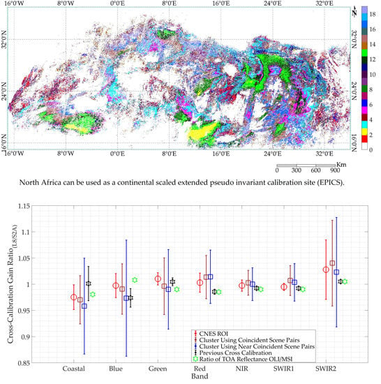
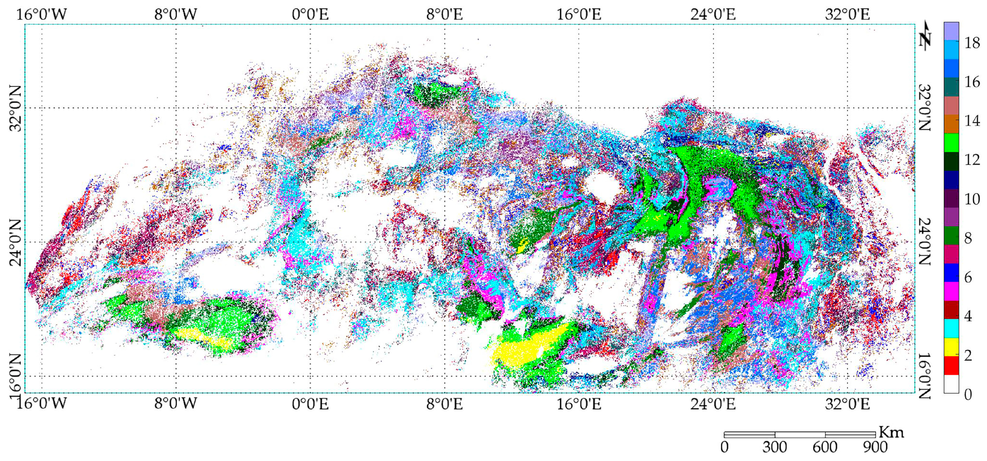
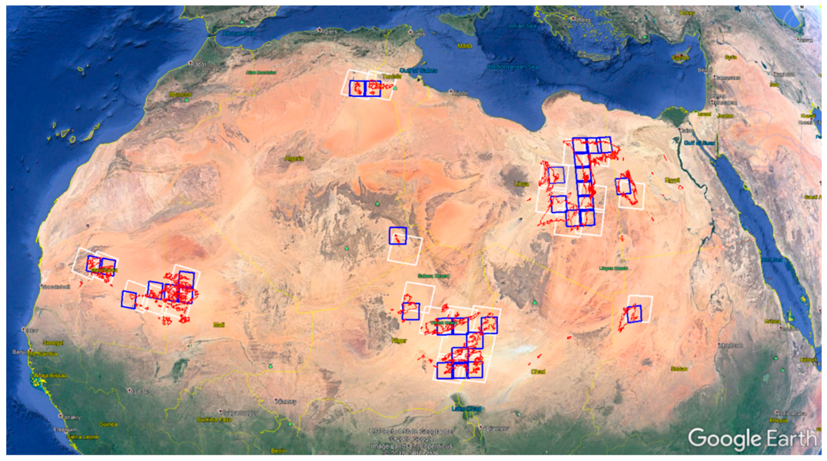
Recently, Shrestha et al. [23] presented an analysis identifying 19 distinct “clusters” with spectrally similar surface cover widespread across North Africa, as shown in Figure 1. These clusters have the potential to provide nearly daily cloud-free imaging by any sensor. Shrestha et al. [24] derived a representative hyperspectral profile for the previously identified clusters based on analysis of the corresponding Earth Observing -1 (EO-1) Hyperion image data. These continental scale clusters help to build a useful cross-calibration dataset within a much reduced time span and also help to reduce the uncertainties in the estimated calibration gains and biases.
This paper describes a methodology for performing EPICS based cross-calibration. The resulting estimated calibration gains and biases, along with their associated uncertainties, are compared to results obtained from the traditional region of interest (ROI)-based cross-calibration approach. For this analysis, the Landsat 8 OLI and Sentinel-2A MSI were chosen as the cross-calibration sensor pair of interest. The analysis was performed using image data from the standard Centre National d’Etudes Spatiales (CNES) ROI within Libya 4 and image data of Shrestha’s Cluster 13 acquired during a one-year interval.
This paper is organized as follows. Section 1 provides a brief overview of the topic. Section 2 discusses the methodology used in the analysis. Section 3 presents the result of the comparison of calibration gain and biased from the two approaches. Section 4 further discusses the result and considers potential directions for future research into this topic. Finally, Section 5 provides a brief summary and conclusions.
2. Data and Methods
A comparison of the traditional ROI-based and proposed cluster-based calibration approaches was performed using Landsat 8 OLI and Sentinel 2A MSI image data. Both sensors have been well calibrated, achieving an absolute radiometric accuracy on the order of 3% and a half-pixel or less in geometric registration uncertainty [4,25]. The key features of the OLI and MSI are summarized in Table 1, with additional descriptions provided below.
2.1. Sensor Description
2.1.1. Landsat 8 OLI
Landsat 8 was launched on 11 February 2013 into a sun-synchronous orbit of 705 km altitude, with a mean equatorial crossing at 10:13 AM local solar time [26]. The OLI, one of two sensors onboard Landsat 8, images solar reflectance across nine spectral bands at spatial resolutions of 30 m in all bands except the panchromatic band, which images at a spatial resolution of 15 m. Its push broom design uses a focal plane containing over 69,000 detectors distributed across 14 distinct modules, allowing it to image a 185 km swath width (corresponding to a 15° field of view).
2.1.2. Sentinel 2A MSI
Sentinel 2A was launched on 23 June 2015 into a sun-synchronous orbit at 786 km altitude, with a mean equatorial crossing at 10:30 am local solar time, close to Landsat 8’s equatorial crossing time. The MSI is also a push broom sensor, imaging solar reflectance across 13 spectral bands with spatial resolutions ranging between 10 m and 60 m. The MSI focal plane detectors are distributed across 12 distinct modules, allowing it to image a 295 km swath width (corresponding to a 20.6° field of view).
2.2. Site and Cluster Selection
2.2.1. Libya 4 Test Site
The Libya 4 Centre National d’Etudes Spatiales (CNES) ROI was selected for performing a traditional ROI-based cross-calibration, as this site has been extensively used for radiometric intercomparison and vicarious calibration of multiple Earth-observing sensors [15,27,28,29,30]. It is regarded as one of the best CNES PICS-based on long term trending of the North African and Arabian deserts.
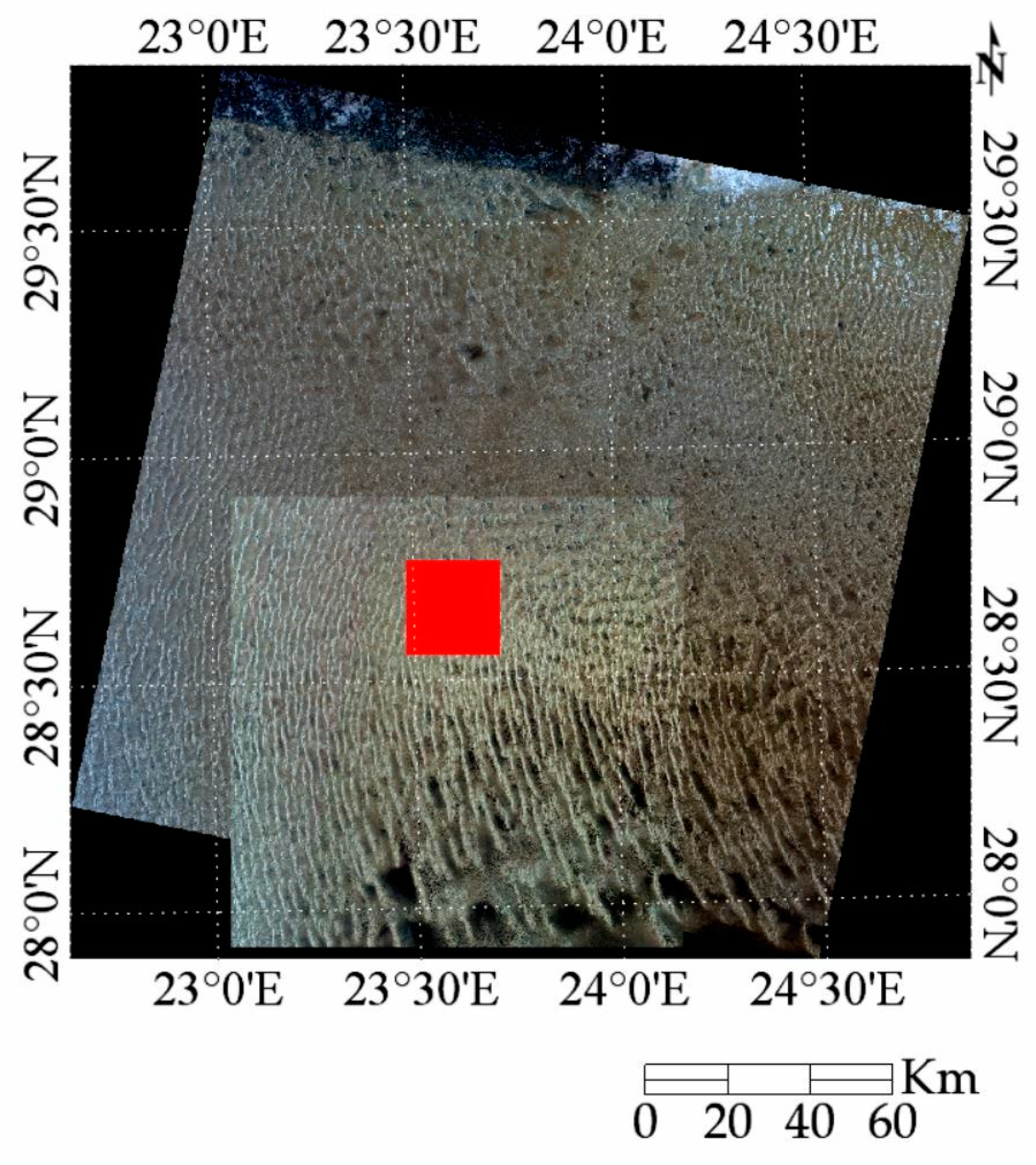
Libya 4 is a high reflectance site in the Saharan desert in North Africa, located at approximately 28.55° N latitude and 23.39° E longitude; it is composed primarily of spatially organized sand dunes. It has demonstrated long-term spatial, spectral, and temporal stability, with a minimum of cloud cover over time [17,31]. Figure 2 shows the general area and specific ROI within Libya 4 in co-located OLI and MSI images.
2.2.2. North African Cluster 13
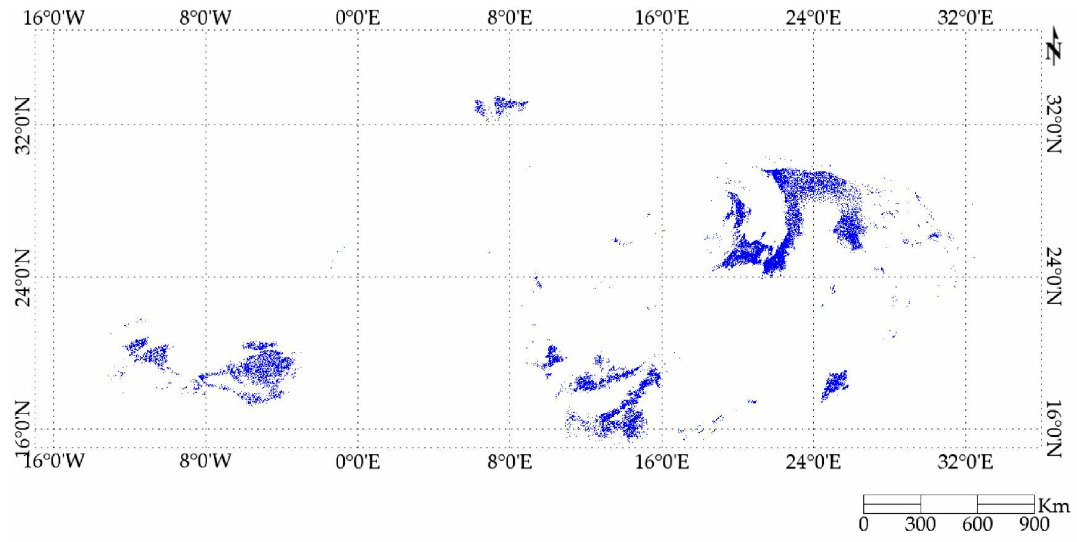
Shrestha et al. [23] performed an unsupervised classification of North Africa based on a 5% maximum temporal uncertainty and identified 19 clusters of distinct surface cover types. The clusters exhibited reflectances of varying intensities with different degrees of spatial stability. Cluster 13 was selected for this cluster-based calibration analysis due to the following: i) it exhibits a spatial uncertainty less than 5% across all bands; ii) it is widely distributed across North Africa, allowing for its imaging on a nearly daily basis as shown in Figure 3 and resulting in an increased number of coincident OLI/MSI scene pairs; and iii) portions of it lie within the Libya 4 and Egypt 1 sites, which provide greater opportunities for hyperspectral imaging as they are frequently observed by the EO-1 Hyperion; this hyperspectral characterization of the surface is mandatory for the accurate compensation of spectral response differences between the OLI and MSI [32].
2.3. Scene Pairs
The Landsat 8 and Sentinel 2A orbits result in different revisit periods (i.e., 16 days for Landsat 8 and 10 days for Sentinel 2A). Consequently, coincident scene pairs between them are acquired every 80 days, with the satellite overpasses typically occurring 16 minutes apart [33]. For this work, the calibration approaches were initially compared using coincident scene pairs; a later comparison included “near coincident” scene pairs (i.e., acquisitions within three days of each other). The three-day window was chosen for the near-coincident pairs under the assumption that no significant changes in surface and atmospheric characteristics had occurred during this period.
After selecting suitable coincident and near coincident scene pairs, Cluster 13 binary masks were generated as described in [34] in order to exclude non Cluster 13 pixels from consideration in the analysis. The remaining pixels were the processed following the procedure described in the following sections.
2.4. Conversion to TOA Reflectance
The OLI image data were converted to TOA reflectance as follows [35]:
where is the solar zenith angle corrected Landsat 8 OLI TOA reflectance; and are, respectively, the band-specific multiplicative and additive scaling factors obtained from the associated product metadata; is the quantized and calibrated standard product pixel value (DN); and is the per-pixel solar zenith angle as extracted from the associated product solar angle band.
The MSI image data were converted to TOA reflectance according to [36]:
where is the MSI TOA reflectance, is the quantized calibrated standard product pixel values (DN), and K is a reflectance scaling factor obtained from the associated product metadata. In this case, the MSI calibrated pixel values account for solar angle effects.
In order to perform a direct reflectance comparison, between the sensors, the spectral difference between them must be addressed. The process used to address this issue is described next.
2.4.1. Spectral Band Adjustment Factor (SBAF)
Two satellite sensors used in a cross-calibration can be designed for very different applications. Based on the application and the existing technology at the time of their development, the sensors will very likely exhibit significant differences in spectral response when observing the same source [32]. Teillet et al. [10] showed that spectral band difference effects are more dependent on surface reflectance characteristics rather than atmospheric conditions or illumination geometry. Such spectral differences can be compensated for if prior knowledge is available concerning the ground target’s spectral signature during the satellite overpass time. Thus, the intrinsic band offset between sensors can be compensated by a target-specific spectral band adjustment factor (SBAF) which takes the target’s spectral profile and the sensor relative spectral responses (RSRs) into account [17,31]. For purposes of this analysis, the OLI was chosen as the calibrated “reference” sensor for SBAF determination. Consequently, the SBAF to be applied to the MSI data to “match” the OLI response was calculated as follows:
where and are, respectively, the simulated TOA reflectances for the OLI and MSI; is a representative hyperspectral profile of the surface; and is the relative spectral response of the corresponding sensor.
Using the derived SBAF, the TOA reflectance of Sentinel 2A MSI is converted to corresponding Landsat 8 OLI TOA reflectance using equation 4.
where is the Sentinel 2A MSI TOA reflectance equivalent to Landsat 8 OLI TOA reflectance.
In order to perform a cross-calibration and cross-comparison between optical satellite sensors, a target-specific SBAF can be derived using an EO-1 Hyperion hyperspectral data or a web-based tool for calculating SBAF from Scanning Imaging Absorption Spectrometer for Atmospheric Chartography (SCHIAMACHY) hyperspectral data. The SCHIAMACHY-based spectral band adjustment factors are computed from algorithms and online tools developed at National Aeronautics and Space Administration Langley Research Center (NASA-LaRC) with SCHIAMACHY V7.01 data obtained from the European Space Agency Envisat program [37,38].
2.4.2. Bidirectional Reflection Distribution Function (BRDF)
Bidirectional reflection distribution function (BRDF) provides the reflectance of the surface as a function of a solar and viewing geometry. Much of the Earth’s surface is non-Lambertian in nature; the reflectance of the surface varies with solar illumination and sensor viewing geometry. BRDF effects increase as the sensor field of view increases; consequently, data from sensors such as the Advanced Very High Resolution Radiometer (AVHRR) and MODIS, with wider fields of view, may require significant BRDF correction [39]. For nadir looking sensors such as the OLI and MSI, the fields of view are relatively narrow (i.e., approximately ±7.5° for the OLI and ±10.3° for the MSI); hence, BRDF effects should be significantly less [40]. Unfortunately, due to differences in viewing and solar illumination geometry between sensors, imaging the same ground target will produce BRDF effects in the image data significant enough to require some level of correction.
Various empirical and semi-empirical BRDF models have been used for addressing BRDF effects in sensor calibration. Liu et al. [41] and Lacherade et al. [30] used Roujean’s semi-empirical BRDF model [42] to remove the angular effect of solar and viewing geometry when performing the cross-calibration of MODIS and Multi-channel Visible Infrared Scanning radiometers (MVIRS). Wu et al. [43] used the Ross-Li semi-empirical BRDF model to remove the angular effect while determining the calibration stability of MODIS using the Libyan Desert and Dome C Antarctic surfaces. Mishra et al. [27] and Helder et al. [28] developed the absolute calibration model using Libya 4 using empirically derived linear and quadratic functions of solar zenith angle to remove the angular effect.
The amount of BRDF correction can be improved by including all four angles, i.e., solar and view zenith and azimuth angles. The development of a full four angle model begins with the conversion of the view and solar angles from a spherical coordinate basis to a linear Cartesian basis in order to obtain TOA reflectance of the surface as a continuous function of independent variables [19]:
where SZA and SAA are the solar zenith and azimuth angles in radians, respectively, and VZA and VAA are the sensor viewing zenith and azimuth angles, respectively (also in radians). Multiple linear least-squares regression is used to derive the models, which account for higher-order and interaction effects between sets of angles.
x1= sin (SZA) * cos (SAA)
y1= sin (SZA) * sin (SAA)
x2 = sin (VZA) * cos (VAA)
y2 = sin (VZA) * sin (VAA)
Once the models have been generated, the mean of solar and sensor view zenith and azimuth angles were chosen as a reference in order to scale the TOA reflectance to a common level. The resulting reference angles were converted to a Cartesian basis, as in (4)–(8), and then used to generate a reference TOA reflectance:
The reference TOA reflectance was then scaled by the ratio of the observed and model-predicted TOA reflectances to obtain the final BRDF-corrected TOA reflectance:
3. Results
This section compares the results of ROI-based and cluster-based cross-calibration between the OLI and the Sentinel 2A MSI. The comparison was performed on coincident and near-coincident scene pairs acquired throughout 2017, and, as both of the sensors were well calibrated, this work assumed that the bias was corrected properly such that the calibration gain could be determined from only bright targets.
3.1. Coincident and Near-Coincident Acquisitions
Due to the orbital patterns of Landsat 8 and Sentinel 2A, only 5.6 percent of the globe offers coincident acquisitions between the OLI and MSI every 80 days [33]. Libya 4 happens to be in the list of specific locations on the Earth’s surface providing such acquisitions. Throughout 2017, four coincident scene pairs were acquired over Libya 4 CNES ROI. Table 2 provides the coincident dates along with the viewing angles for each sensor.
As Cluster 13 extends across North Africa (Figure 3), it increases the opportunity to collect coincident acquisitions between Landsat 8 and Sentinel 2A. Figure 4 shows the intersections between the Cluster 13 boundaries (red boxes) and the Landsat 8 and Sentinel 2A footprints (the white boxes and blue boxes, respectively). 28 locations intersect Cluster 13 and each sensor’s footprints. Among these paths and rows, only six paths and rows have cloud-free acquisitions coincident acquisitions, as shown in Table 3.
Similarly, Libya 4 CNES ROI has eight near coincident acquisitions between Landsat 8 OLI and Sentinel 2A, as listed in Table 4. Acquisitions that are three days apart are considered as near coincident, since the surface properties and atmosphere do not change significantly within this short temporal window; Barsi et al. [44] have shown that Libya 4 CNES ROI is very stable over a six day time period for cloud-free acquisitions, which they consider suitable for cross-calibration purposes.
Similarly, Cluster 13 offers 108 cloud-free scene pairs from 20 Worldwide Reference System (WRS)-2 paths and rows. The significant increase in near-coincident scene pairs usable for cluster-based cross-calibration is possible due to its widespread spatial distribution across North Africa.
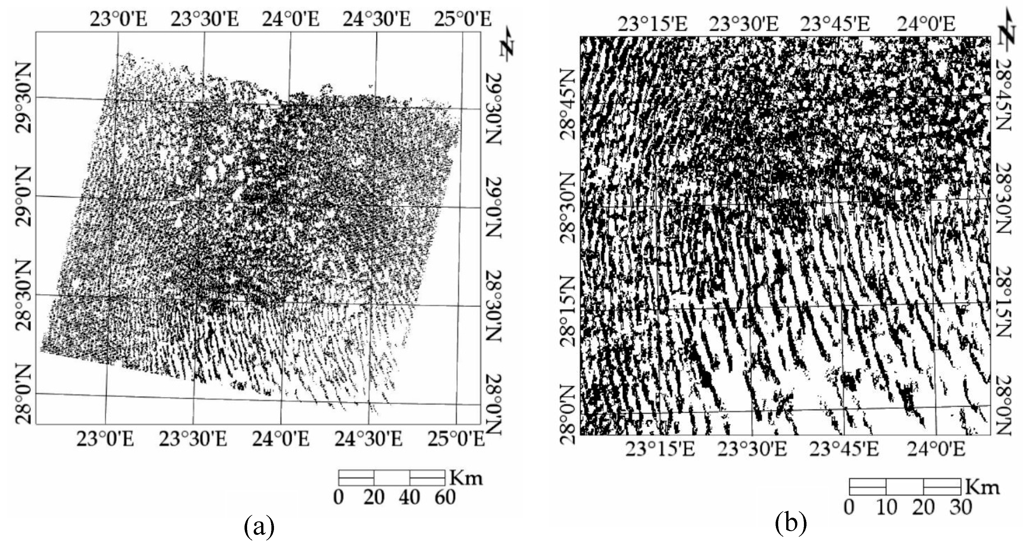
After getting the cloud-free coincident and near-coincident scene pairs, OLI and MSI TOA reflectances were calculated from pixels within the CNES ROI for the traditional PICS-based calibration approach. For the cluster-based approach, the reflectances were calculated from the pixels within a region common to Cluster 13 and each sensor’s footprint, as shown in Figure 5.
Once the TOA reflectances for each sensor were determined, the SBAF was applied to compensate for spectral response differences between the sensors. The next section shows the resulting SBAF distributions for the MSI.
3.2. SBAF for Libya 4 CNES ROI and Cluster 13
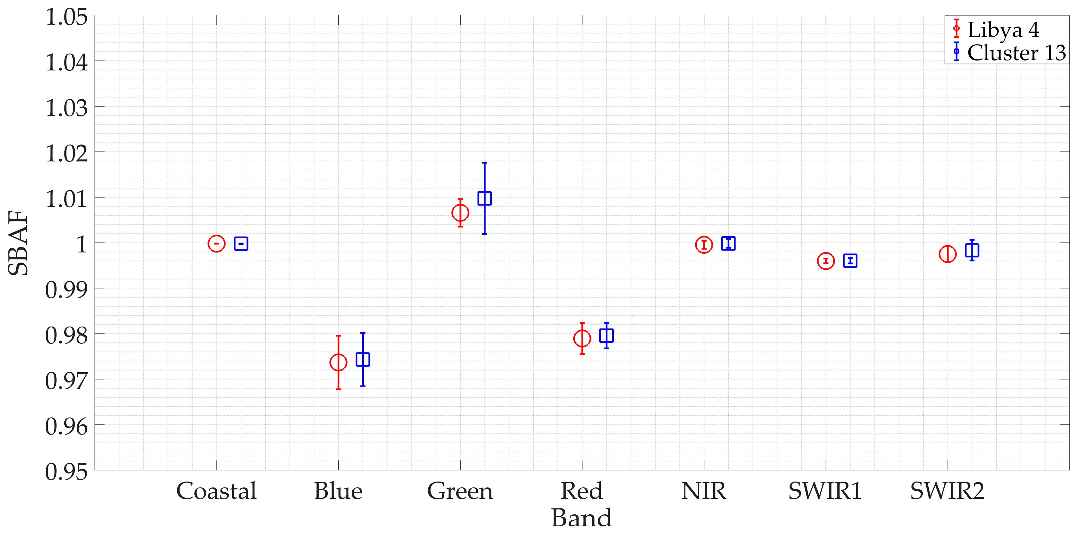
For this work, the OLI was considered as the reference to which the MSI spectral response is normalized. Libya 4 has sets of SBAFs derived from 59 hyperspectral data profiles, whereas Cluster 13 has sets of SBAFs estimated from 188 hyperspectral profiles [24]. Figure 6 shows the resulting MSI SBAF (2 sigma) for all common bands.
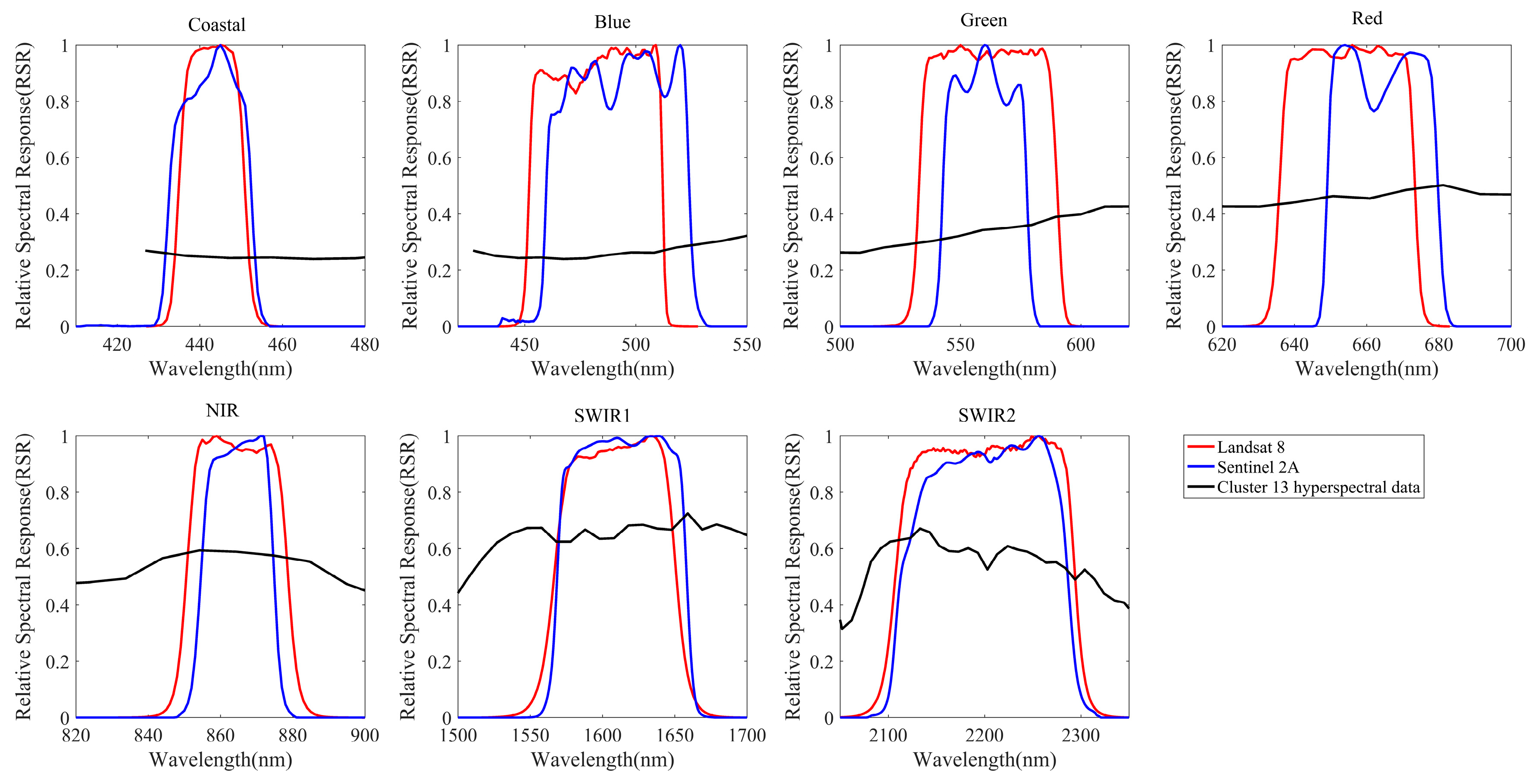
Since Libya 4 is included within Cluster 13 [23,24], the SBAFs for Libya 4 CNES ROI and Cluster 13 were similar to each other. The RSR’s of coastal, NIR, SWIR 1, and SWIR 2 bands of these two sensors were very similar to each other, as shown in Appendix A, which resulted in an SBAF very close to one. In contrast, the SBAF for the blue and red bands differed from one because their RSR’s were shifted relative to each other. In addition, the MSI SBAF mean values for both Libya 4 CNES ROI and Cluster 13 were equal for all bands except the green band, and the observed 0.35% difference was due to more discrepancy between the hyperspectral profiles of Libya 4 CNES ROI and Cluster 13 from 500 to 560 nm; some of it is presumably due to the difference in width of the RSR’s of the two sensors [44]. Such a relative shift and width mismatch of the RSR between the two sensors also contributed to the higher SBAF uncertainty of the blue, green, and red bands, as shown in Figure 6. The SBAF uncertainty of the blue band was approximately 0.25% and similar for both CNES ROI and Cluster 13, whereas the SBAF uncertainty of the green band using Cluster 13 was larger by 0.24% than using the CNES ROI.
The mean SBAF difference was as large as 3.5% and 2.5% for the blue and red bands, respectively, because the OLI and MSI RSR’s in these bands were shifted relative to each other with respect to hyperspectral signature of the target, as shown in Appendix A.
3.3. Comparison of TOA Reflectance of Landsat 8 and Sentinel 2A
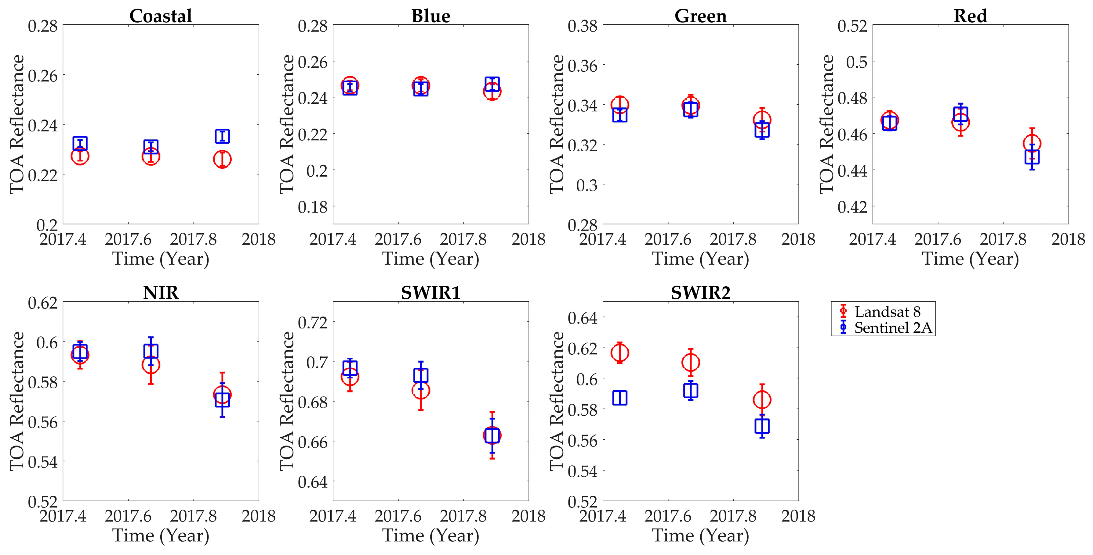
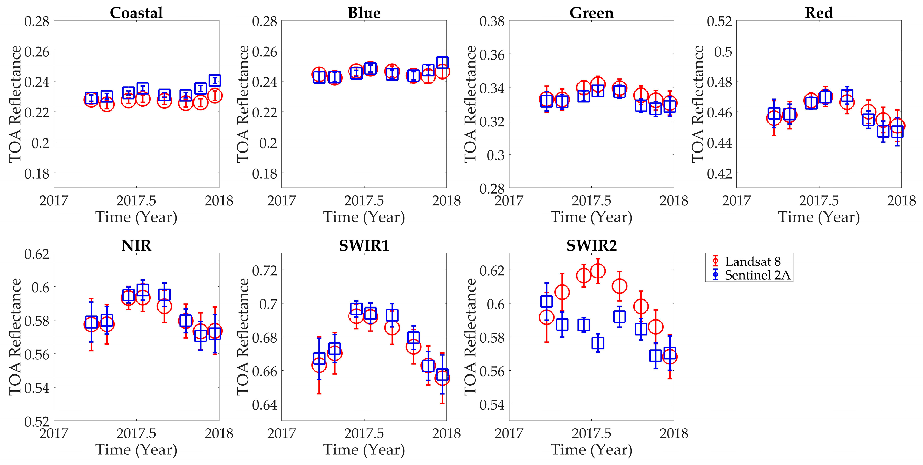
After performing SBAF and BRDF correction to the MSI TOA reflectance, OLI and MSI TOA reflectances were compared with each other. The comparison of Landsat 8 OLI and Sentinel 2A MSI TOA reflectance (2 sigma) using Libya 4 CNES ROI coincident scene pairs is presented in Figure 7 (traditional ROI-based approach) and Figure 8 (cluster-based approach). The estimated Libya 4 CNES ROI TOA reflectances from both ROI and cluster-based methods were consistent with each other. As expected, the VNIR and SWIR1 band TOA reflectances from both sensors were in better agreement than in the SWIR 2 band, suggesting there are residual spectral differences were not accounted for with the SWIR2 SBAF correction.
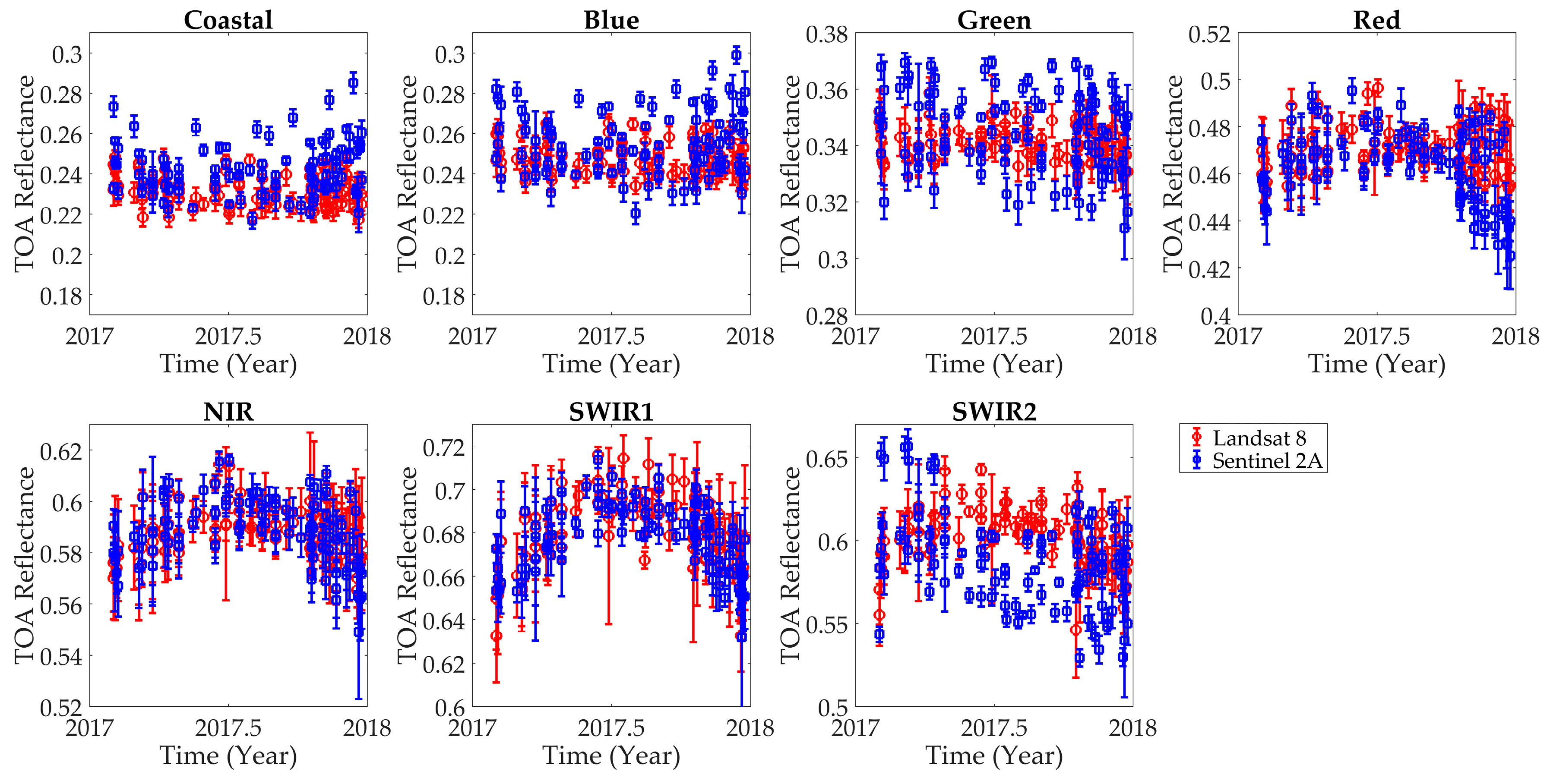
The comparison of OLI and MSI TOA reflectance using near-coincident scene pairs are presented in Figure 9 (traditional ROI-based approach) and Figure 10 (cluster-based approach). As with the coincident scene pairs, the reflectances were consistent for both approaches and lied with each other’s uncertainty for all bands except the SWIR 2 band. In Figure 10, the observed TOA reflectance uncertainty, such as approximately 5% for the coastal band and approximately 3% for the NIR band, was expected and equivalent to the spatial uncertainty (ratio of spatial standard derivation to spatial mean) of Cluster 13, as it was the main source of uncertainty. As in the previous comparison using coincident scene pairs, the SWIR 2 band had more discrepancy between the TOA reflectance of OLI and MSI than the rest of the bands.
3.4. Comparison of Cross-Calibration Gain Ratios from ROI-Based and Cluster-Based Approach
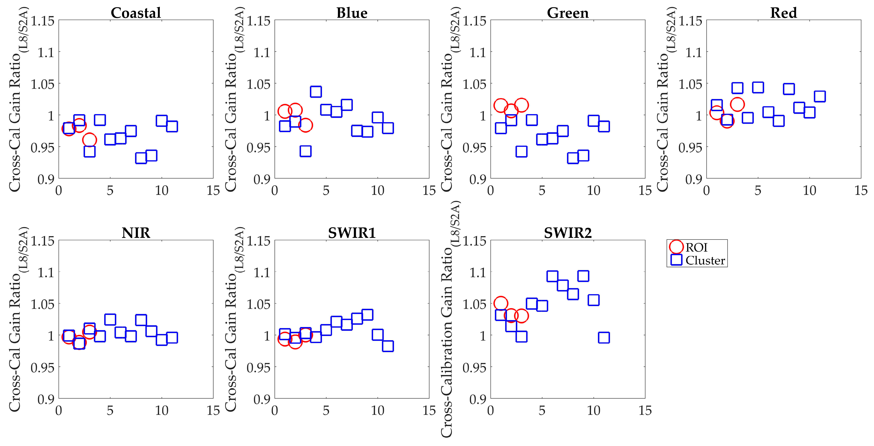
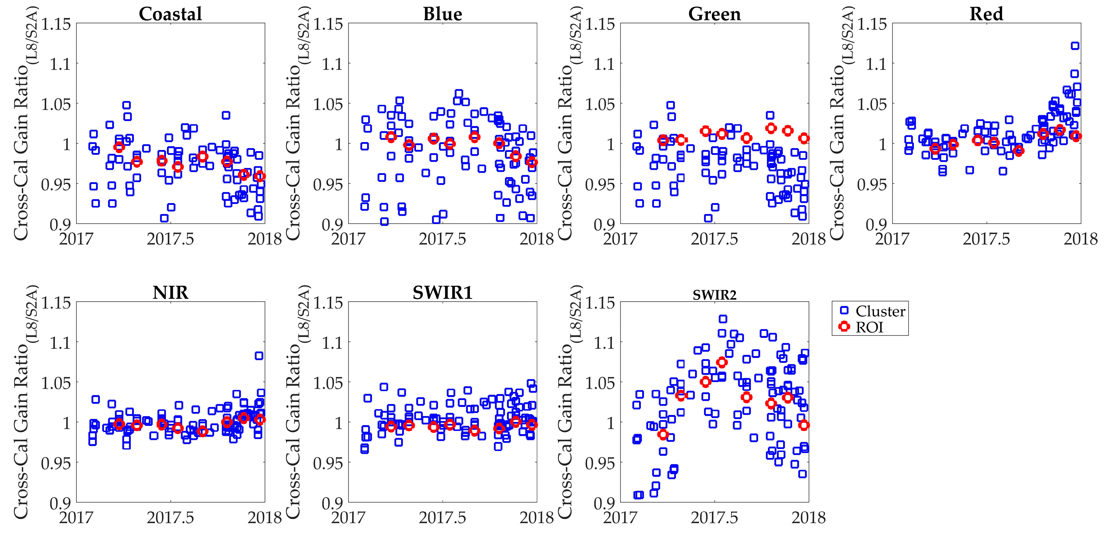
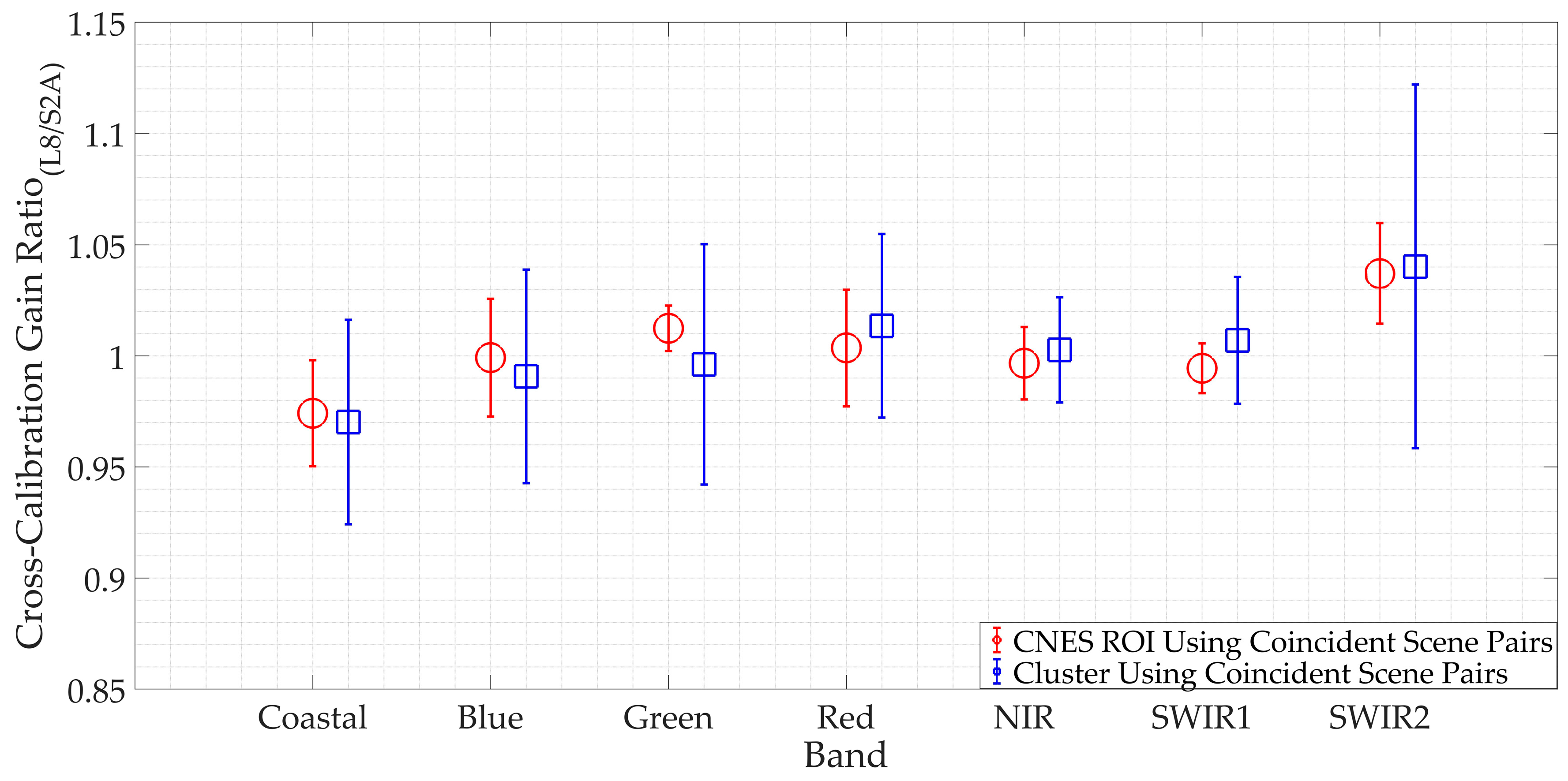
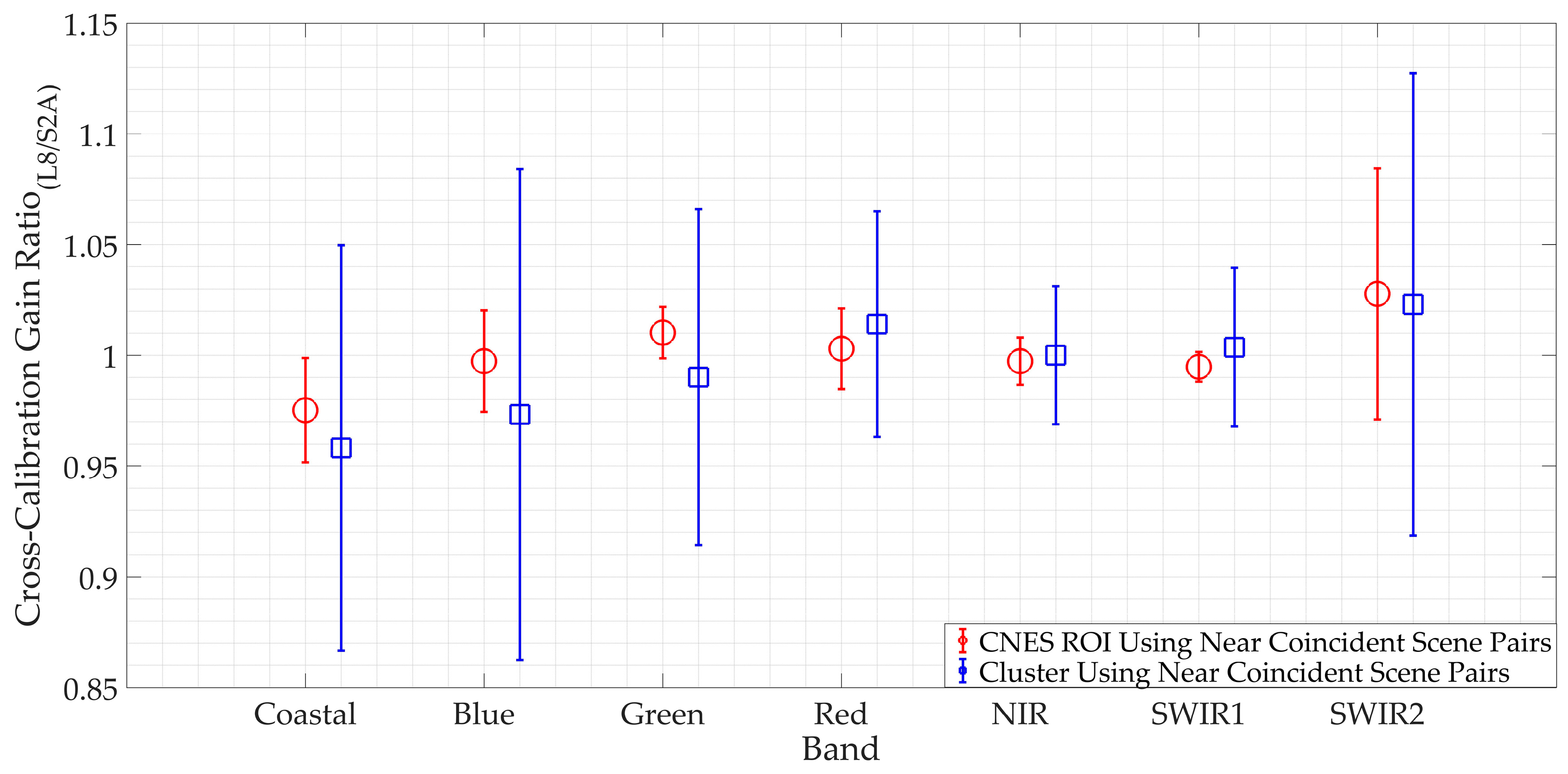
After correcting the MSI TOA reflectances, the cross-calibration gain ratio was calculated as the ratio of OLI TOA reflectance to MSI TOA reflectance, as shown in Figure 11 (for 3 coincident scene pairs from Libya 4 CNES ROI and 11 coincident scene pairs from the 6 WRS-2 paths/rows within Cluster 13) and Figure 12 (for 8 near-coincident scene pairs from Libya 4 CNES ROI and 108 near-coincident scene pairs from the 20 WRS-2 paths/rows within Cluster 13). In these figures, the red symbols represent the cross-calibration gain ratios derived from the traditional ROI-based cross-calibration method, whereas the blue symbols represent the cross-calibration gain ratios derived from the cluster-based approach.
As Cluster 13 also includes Libya 4 CNES ROI, the cluster-based and ROI-based cross-calibration gain ratios were similar to each other. The cross-calibration gain ratios derived from the traditional ROI-based approach using coincident scene pairs tended to exhibit less scatter than the corresponding gain ratios derived from the cluster-based approach, as the Libya 4 CNES ROI had less uncertainty than Cluster 13. Figure 11 and Figure 12 show that, among all the bands, the cross-calibration gain ratios of the NIR band were more consistent, as both of the sensors had very good agreement on their TOA reflectance; there was only 1.56% variability using cluster-based near coincident scene pair. In contrast, the cross-calibration gain ratios of the SWIR 2 band had the maximum variability of approximately 5% (using cluster-based near coincident scene pairs) as the TOA reflectance from OLI and MSI had a broader range in this band, as presented in Figure 8 and Figure 10.
Figure 13 and Figure 14, respectively, represent the mean cross-calibration gain ratio and associated standard deviation derived for both cross-calibration approaches. The mean cross-calibration gain ratio was calculated by taking an average of temporal cross-calibration gain ratios, as shown in Figure 11 and Figure 12, and plotted with its corresponding 2-sigma standard deviation in Figure 13 and Figure 14. Ideally, after application of the SBAF and BRDF corrections, the cross-calibration gain ratios for two well-calibrated sensors should have been equal to 1. The cross-calibration gain ratios derived from both approaches deviated from 1 due to the sensor absolute radiometric uncertainty, uncertainties associated with the SBAF and BRDF corrections themselves, and uncertainties due to the atmosphere. In general, both approaches tend to produce consistent cross-calibration gain ratio estimates. The cross-calibration gain ratio derived from the cluster-based approach had consistently higher uncertainty across all the bands. Though the green band had a lower spatial uncertainty (3%) than the coastal and blue bands (5%), the cross-calibration gain ratio had a similar uncertainty. In general, the error bars of the cross-calibration gain ratio derived from both methods overlapped, implying that the cluster-based cross-calibration provided consistent results with the ROI-based cross-calibration approach.
Figure 14 shows that the cross-calibration gain ratios derived from the cluster-based approach were similar to the cross-calibration gain ratios derived from an ROI-based approach but are not consistent, as they have higher uncertainty across all the bands. The cross-calibration gain ratio for shorter wavelengths had higher uncertainty than the longer wavelength as the spatial uncertainty of Cluster 13 was higher in the shorter wavelengths than the rest of the bands. The cross-calibration gain ratios of the blue and NIR bands had the highest and lowest uncertainty of approximately 11% and 3%, respectively. For the SWIR 2 band, both sensors appeared to exhibit inherently more variation in TOA reflectance than in the other bands, increasing the uncertainty in cross-calibration gain ratio estimated with both approaches. Though the larger number of scene pairs available with the cluster-based approach tended to average out the random BRDF and atmospheric effects, resulting in a more accurate cross-calibration gain estimate, the spatial uncertainty of Cluster 13 drove up the cross-calibration gain uncertainty.
4. Discussion
PICS have been extensively used by multiple researchers for sensor inter-comparison and cross-calibration [11,12,17,18]. In cross-calibration, the response of one sensor is compared with the response of another well-calibrated sensor using coincident and/or near-coincident scene pairs of a selected area on the Earth’s surface. Traditionally, a limited number of spatially and temporally stable regions in North Africa with corresponding hyperspectral information were used for sensor cross-calibration. Given limitations in imaging frequently due to sensor revisit time and the occurrence of adverse cloud cover potentially obscuring the site, a much longer time period is required to acquire suitable coincident and/or near-coincident cross-calibration scene pairs. This is the major limitation of the existing ROI-based cross-calibration method.
Recently, Shrestha et al. [23,24] found 19 distinct “clusters” of spectrally similar surface cover throughout North Africa, which can be considered temporally and spatially stable. They also estimated a representative hyperspectral profile of these clusters for use as EPICS targets suitable for sensor cross-calibration purposes. These clusters are distributed across the continent such that they can be imaged on a daily or nearly a daily basis by any satellite sensor. Since these EPICS are more frequently imaged than an individual PICS, the number of candidate cross-calibration opportunities using coincident and near coincident scene pairs increases significantly.
As clusters provide a larger number of coincident scene pairs, the current work focused on developing a technique to use EPICS for cross-calibration purposes. To analyze this technique, two individually well-calibrated sensors, the Landsat 8 OLI and Sentinel 2A MSI, were chosen, and a single year time frame was selected for the test purpose. Libya 4 CNES ROI was selected as a representative “traditional” PICS, as its temporal and spatial stability has been well established in earlier work. Shrestha’s Cluster 13 was chosen, as it is widely distributed across North Africa and possesses lower spatial uncertainty across all bands. Cluster 13 also includes Libya 4 CNES ROI, thus facilitating comparison between the traditional ROI-based approach and the proposed cluster-based cross-calibration approach.
For this work, the near-coincident scene pairs were acquired approximately three days apart. For such a short time interval, it can be assumed that surface response does not appreciably change. Furthermore, Barsi et al. [44] showed that Libya 4 CNES ROI was temporally and spatially stable over a six day period, assuming cloud-free conditions. Consequently, image pairs did not necessarily need to be acquired on the same date to be considered for cross-calibration purposes. Even using a spatial extent of Cluster 13, there were only 11 coincident scene pairs due to the sensor revisit time and imaging schedules.
OLI and MSI TOA reflectance from Libya 4 CNES ROI exhibits some random variations about a mean value but are very consistent, using both coincident and near coincident scene pairs as shown in Figure 7 and Figure 8. The TOA reflectance from these two sensors lies within each other’s uncertainty range for all bands except the SWIR 2 band. Within the study period, it had a maximum difference between the TOA reflectance of CNES ROI of an approximately 0.04 reflectance unit for both using coincident and near-coincident scene pairs. One of the reasons for these observed differences was due to spectral difference not accounted by SBAF corrections, and another reason was the change in the site or a sensor with respect to time. Barsi et al. [44] showed that both OLI and MSI have positive slopes of TOA reflectance over time using data from June 2015 to May 2017, which might have contributed to the observed TOA reflectance in Figure 7 and Figure 8.
Figure 9 and Figure 10 show the comparison of OLI and MSI TOA reflectance of Cluster 13 using coincident and near-coincident scene pairs. The TOA reflectance of both the sensors had less variation using coincident scene pairs than using near-coincident scene pairs because only six locations of Cluster 13 offered coincident scene pairs between the two sensors, whereas 20 locations offered the near-coincident scene pairs, which increase the likelihood of higher spatial uncertainty. For example, the TOA reflectance of the coastal band had a difference of 0.02 reflectance using only coincident scene pairs, whereas it had a difference of 0.04 reflectance while using near-coincident scene pairs. The change of 0.04 absolute reflectance was approximately 16% (3 sigma) in a relative scale. The spatial uncertainty of Cluster 13 was approximately 5% (1 sigma), which would be equivalent to the change in variation that is being observed. As such, the observed amount of variation in TOA reflectance using the near-coincident scene pairs is expected in a cluster-based approach.
As this is an initial attempt to use EPICS for cross-calibration, the cross-calibration gain ratio was calculated simply by taking the ratio of TOA reflectance of two sensors for each band. The cross-calibration gain ratio derived using both coincident and near-coincident scene pairs had variation as expected due to a Cluster 13 spatial uncertainty of approximately 5% in the coastal and blue bands and 3% for the rest of the bands, as shown in Figure 11 and Figure 12. Using coincident scene pairs, the uncertainty of the cluster-based cross-calibration gain ratio was within 3 % for all the bands except for the SWIR 2 band, as shown in Figure 13. When using near coincident scene pairs, the uncertainty was within 5% for all bands except the Blue and SWIR2 bands, as shown in Figure 14. Note that Cluster 13 has 11 coincident scene pairs obtained from 6 WRS-2 paths/rows and 108 near coincident scene pairs are obtained from 20 paths/rows. The increased uncertainty in calibration gain derived using near coincident scene pair was more due to spatial uncertainty of Cluster 13 than the three-day window used to consider the acquisition as near coincident scene pairs.
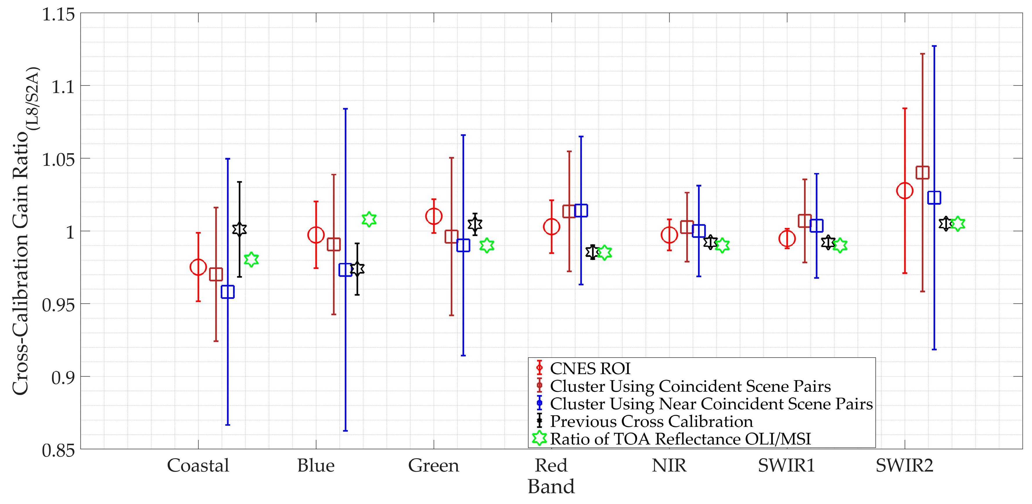
As the purpose of this work was to demonstrate the technique of using cluster-based cross-calibration, a comparison was made between the cross-calibration gain ratio using the Libya 4 CNES ROI, Cluster 13, and the cross-calibration gain using lifetime data of the OLI and Sentinel 2A MSI at different locations [19]. The cross-calibration gain ratio obtained from this work was compared with the calibration gains obtained by Farhad [19]. Figure 15 shows the estimated cross-calibration gain ratio between the OLI and Sentinel-2A MSI for each band. The red symbols represent the cross-calibration gain ratios obtained by using the eight near coincident scene pairs of the Libya 4 CNES ROI. The brown symbols represent the cross-calibration gain ratio obtained by using the 11 coincident scene pair of Cluster 13, and the blue symbols represent the cross-calibration gain ratio obtained by using the 108 near coincident scene pairs of Cluster 13. The green symbols represent the average lifetime ratios for the common spectral bands of OLI and MSI using Libya 4 CNES ROI; six acquisitions collected on the same day and 28 acquisitions collected up to six days apart [44]. Finally, the black symbols represent the estimated calibration gains using the traditional ROI-based method using PICS with varying intensity levels [19]. In general, the cross-calibration gain ratios obtained in this work using Cluster 13 are consistent with the calibration gains obtained by Farhad. The NIR band had the best agreement between the mean values of cross-calibration gain, as all of them were within 1%. In the coastal/aerosol band, there was a maximum offset of approximately 4% between the mean cross-calibration gain values that was more likely due to the spatial uncertainty of Cluster 13. The cluster-based mean cross-calibration gain ratio of SWIR 2 band had an offset of approximately 4% using coincident scene pairs and 2.5% using near coincident scene pair (assuming the cross calibration gain ratio should be 1 as both of the sensors are well calibrated), which was also most likely due to the greater uncertainties in TOA reflectance for these sensors in this spectral region. A similar amount of differences was observed between the cross-calibration gain ratios using the cluster-based approach and the cross-comparison results across all spectral regions [44]. Despite some discrepancy, the cluster-based cross-calibration gain ratio encompassed the cross-calibration gain values obtained by previous cross-calibration works, which implies that the cross-calibration gain ratio obtained from these different approaches are statistically indistinguishable.
Along with the spatial uncertainty within the Cluster 13 regions, atmospheric uncertainty and uncertainty due to BRDF effects also contribute to the overall cross-calibration gain uncertainty. Atmospheric effects are believed to contribute 1–2% towards the overall uncertainty [28]. The MSI field of view (FOV) was approximately 20° vs 15° for the OLI, and the view zenith angle was approximately 2.5° more than the OLI’s (10° vs 7.5°); in some extreme cases, the viewing angles could differ up to 20° [45]. Gao et al. [46] concluded that for sensors with narrower FOVs (such as the OLI and MSI), the major BRDF effects result from variation in solar illumination, which is date-dependent. These types of angular effects in TOA reflectance can be corrected, but a narrow angular sampling of moderate resolution sensors complicates BRDF coefficient retrieval, potentially limiting the degree of BRDF correction in the image data, particularly at shorter wavelengths. However, for longer-wavelength bands where atmospheric effects are reduced and BRDF correction is adequate (such as the NIR and SWIR1 bands), the cluster-based calibration gains are more consistent with previously cross-calibration results, despite the greater uncertainty.
From the above discussion, it is clear that the cluster-based calibration gains are comparable to the results of previous cross-calibration works in terms of accuracy but currently exhibit greater uncertainty. This suggests that the cluster-based cross-calibration approach can deliver results consistent with traditional ROI-based cross-calibration results once the uncertainty is properly considered. In addition to efforts to reduce overall uncertainty, future work could include using multiple clusters with varying intensity levels different than Cluster 13 so that both cross-calibration gain and bias can be observed. In order to minimize random noise in the cross-calibration gain ratio, it could be calculated using the lifetime mean TOA reflectance data of both sensors instead of using individual coincident and near coincident scene pairs.
5. Conclusions
This article presents the methodology for a cluster-based cross-calibration of optical satellite sensors. The cluster-based calibration uses spectrally similar regions, such as Cluster 13, for finding coincident scene pairs. Since these regions are widely spread across North Africa, it offers a significantly increased number of cross-calibration opportunities as compared to the traditional ROI-based approach from distinct PICS. The greater number of cross-calibration opportunities helps to average out random errors and estimate more accurately the calibration gains between sensors.
Cluster 13 was chosen to demonstrate the methodology because it has a large number of contiguous regions widely distributed across North Africa and it includes the well-known Libya 4 PICS (CNES ROI) which has been extensively used for radiometric calibration purposes. Two well-calibrated sensors, the Landsat 8 OLI and Sentinel 2A MSI, were chosen as the sensor pair. The comparison was performed using image data acquired in 2017. For these sensors during this time period, Libya 4 CNES ROI offered just three coincident and eight near coincident cloud-free scene pairs; on the other hand, Cluster 13, which includes Libya 4 CNES ROI, offered 11 coincident and 108 cloud free near coincident scene pairs.
The results of this work indicate that, for most bands, a cluster-based cross-calibration approach produces similar results to the traditional ROI-based cross-calibration result. Using coincident scene pairs, the cluster-based cross-calibration gain ratio was within 2% of the gain derived from previous ROI-based cross calibration gain for all bands except the coastal and SWIR 2 bands. The difference in the SWIR 2 band gain was most likely due to greater uncertainty in TOA reflectance of both sensors. Similarly, with the near-coincident scene pairs, the cluster-based cross-calibration gain difference was within 2% for most of the bands but exhibited greater uncertainty, by 2%, than that of the ROI-based method at this time. The greater uncertainty was mainly due to spatial uncertainty within Cluster 13 regions, which was approximately 4% for the coastal band; some of the overall uncertainty was also due to residual atmospheric and BRDF effects. However, despite the greater uncertainty, the cross-calibration gain ratio estimated with the cluster-based approach had similar accuracy with the cross-calibration gain ratio derived from the traditional ROI-based approach.
The use of EPICS clusters can significantly increase the number of cross-calibration opportunities within a much shorter time period. Based on these results, any region within Cluster 13 could, in principle, be used for sensor cross-calibration purposes; the level of accuracy provided by the proposed method is comparable to that provided by the traditional ROI-based method.
Author Contributions
M.S. conceived the research and developed the algorithm with the help of L.L. and D.H. M.S., L.L., and D.H. analyzed the data. M.N.H. generated binary mask to filter in the desired pixel of a cluster. M.S. wrote the paper. L.L. and D.H. edited the paper.
Funding
This research was funded by NASA (grant number NNX15AP36A) and USGS EROS (grant number G14AC00370).
Acknowledgments
The authors would like to thank Tim Ruggles for editing the manuscript and reviewers for their comments that improved the quality of this paper.
Conflicts of Interest
The authors declare no conflict of interest.
Appendix A
In this appendix, we include the RSR comparison of different bands of Landsat 8 OLI and Sentinel 2A MSI.
Figure A1.
Relative Spectral Response (RSR) of Landsat 8 OLI and Sentinel 2A.

References
- Slater, P.N.; Biggar, S.F.; Palmer, J.M.; Thome, K.J. Unified approach to absolute radiometric calibration in the solar-reflective range. Remote Sens. Environ. 2001, 77, 293–303. [Google Scholar] [CrossRef]
- Dinguirard, M.; Slater, P.N. Calibration of space-multispectral imaging sensors: A review. Remote Sens. Environ. 1999, 68, 194–205. [Google Scholar] [CrossRef]
- Thome, K.; Markharn, B.; Barker, P.S.; Biggar, S. Radiometric calibration of Landsat. Photogramm. Eng. Remote Sens. 1997, 63, 853–858. [Google Scholar]
- Markham, B.; Barsi, J.; Kvaran, G.; Ong, L.; Kaita, E.; Biggar, S.; Czapla-Myers, J.; Mishra, N.; Helder, D. Landsat-8 operational land imager radiometric calibration and stability. Remote Sens. 2014, 6, 12275–12308. [Google Scholar] [CrossRef]
- Slater, P.; Biggar, S.; Holm, R.; Jackson, R.; Mao, Y.; Moran, M.; Palmer, J.; Yuan, B. Reflectance-and radiance-based methods for the in-flight absolute calibration of multispectral sensors. Remote Sens. Environ. 1987, 22, 11–37. [Google Scholar] [CrossRef]
- Thome, K. Absolute radiometric calibration of Landsat 7 ETM+ using the reflectance-based method. Remote Sens. Environ. 2001, 78, 27–38. [Google Scholar] [CrossRef]
- Thome, K.J.; Gustafson-Bold, C.; Slater, P.N.; Farrand, W.H. In-Flight Radiometric Calibration of Hydice Using a Reflectance-Based Approach; Hyperspectral Remote Sensing and Applications, 1996; International Society for Optics and Photonics: Bellingham, WA, USA, 1996; pp. 311–320. [Google Scholar]
- Teillet, P.; Slater, P.; Ding, Y.; Santer, R.; Jackson, R.; Moran, M. Three methods for the absolute calibration of the NOAA AVHRR sensors in-flight. Remote Sens. Environ. 1990, 31, 105–120. [Google Scholar] [CrossRef]
- Czapla-Myers, J.; McCorkel, J.; Anderson, N.; Thome, K.; Biggar, S.; Helder, D.; Aaron, D.; Leigh, L.; Mishra, N. The ground-based absolute radiometric calibration of Landsat 8 OLI. Remote Sens. 2015, 7, 600–626. [Google Scholar] [CrossRef]
- Teillet, P.; Barker, J.; Markham, B.; Irish, R.; Fedosejevs, G.; Storey, J. Radiometric cross-calibration of the Landsat-7 ETM+ and Landsat-5 TM sensors based on tandem data sets. Remote Sens. Environ. 2001, 78, 39–54. [Google Scholar] [CrossRef] [Green Version]
- Chander, G.; Angal, A.; Choi, T.J.; Meyer, D.J.; Xiong, X.J.; Teillet, P.M. Cross-Calibration of the Terra MODIS, Landsat 7 ETM+ and EO-1 ALI Sensors Using Near-Simultaneous Surface Observation over the Railroad Valley Playa, Nevada, Test Site; Earth Observing Systems XII, 2007; International Society for Optics and Photonics: Bellingham, WA, USA, 2007; p. 66770Y. [Google Scholar]
- Chander, G.; Meyer, D.J.; Helder, D.L. Cross calibration of the Landsat-7 ETM+ and EO-1 ALI sensor. IEEE Trans. Geosci. Remote Sens. 2004, 42, 2821–2831. [Google Scholar] [CrossRef]
- Cosnefroy, H.; Briottet, X.; Leroy, M.; Lecomte, P.; Santer, R. In Field Characterization of Saharan Sites Reflectances for the Calibration of Optical Satellite Sensors. In Proceedings of the IGARSS’94-1994 IEEE International Geoscience and Remote Sensing Symposium, Pasadena, CA, USA, 8–12 August 1994; IEEE: Piscataway, NJ, USA, 1994; pp. 1500–1502. [Google Scholar]
- Cosnefroy, H.; Leroy, M.; Briottet, X. Selection and characterization of Saharan and Arabian desert sites for the calibration of optical satellite sensors. Remote Sens. Environ. 1996, 58, 101–114. [Google Scholar] [CrossRef]
- Bouvet, M. Radiometric comparison of multispectral imagers over a pseudo-invariant calibration site using a reference radiometric model. Remote Sens. Environ. 2014, 140, 141–154. [Google Scholar] [CrossRef]
- Helder, D.L.; Basnet, B.; Morstad, D.L. Optimized identification of worldwide radiometric pseudo-invariant calibration sites. Can. J. Remote Sens. 2010, 36, 527–539. [Google Scholar] [CrossRef]
- Chander, G.; Mishra, N.; Helder, D.L.; Aaron, D.B.; Angal, A.; Choi, T.; Xiong, X.; Doelling, D.R. Applications of spectral band adjustment factors (SBAF) for cross-calibration. IEEE Trans. Geosci. Remote Sens. 2013, 51, 1267–1281. [Google Scholar] [CrossRef]
- Chander, G.; Angal, A.; Choi, T.; Xiong, X. Radiometric cross-calibration of EO-1 ALI with L7 ETM+ and Terra MODIS sensors using near-simultaneous desert observations. IEEE J. Sel. Top. Appl. Earth Obs. Remote Sens. 2013, 6, 386–399. [Google Scholar] [CrossRef]
- Farhad, M.M. Cross Calibration and Validation of Landsat 8 OLI and Sentinel 2A MSI. Master’s Thesis, South Dakota State University, Brookings, SD, USA, 2018. [Google Scholar]
- Pinto, C.; Ponzoni, F.; Castro, R.; Leigh, L.; Mishra, N.; Aaron, D.; Helder, D. First in-flight radiometric calibration of MUX and WFI on-board CBERS-4. Remote Sens. 2016, 8, 405. [Google Scholar] [CrossRef]
- Li, S.; Ganguly, S.; Dungan, J.L.; Wang, W.; Nemani, R.R. Sentinel-2 MSI radiometric characterization and cross-calibration with Landsat-8 OLI. Adv. Remote Sens. 2017, 6, 147. [Google Scholar] [CrossRef]
- Doelling, D.; Helder, D.; Schott, J.; Stone, T.; Pinto, C. Vicarious Calibration and Validation. In Comprehensive Remote Sensing; Liang, S., Ed.; Elsevier: Oxford, UK, 2018; Volume 1, pp. 475–518. [Google Scholar]
- Shrestha, M.; Leigh, L.; Helder, D. Classification of the North Africa Region for Use as an Extended Pseudo Invariant Calibration Sites (EPICS) for Radiometric Calibration and Stability Monitoring of Optical Satellite Sensors. Remote Sens. 2019, 11, 875. [Google Scholar] [CrossRef]
- Shrestha, M.; Leigh, L.; Helder, D.; Loveland, T. Large area Saharan PICS developemnt for calibration and stability monitoring of optical satellite sensors. In Proceedings of the Pecora 20, Sioux Falls, SD, USA, 13–16 November 2017. [Google Scholar]
- Gascon, F.; Bouzinac, C.; Thépaut, O.; Jung, M.; Francesconi, B.; Louis, J.; Lonjou, V.; Lafrance, B.; Massera, S.; Gaudel-Vacaresse, A. Copernicus Sentinel-2A calibration and products validation status. Remote Sens. 2017, 9, 584. [Google Scholar] [CrossRef]
- Irons, J.R.; Dwyer, J.L.; Barsi, J.A. The next Landsat satellite: The Landsat data continuity mission. Remote Sens. Environ. 2012, 122, 11–21. [Google Scholar] [CrossRef]
- Mishra, N.; Helder, D.; Angal, A.; Choi, J.; Xiong, X. Absolute calibration of optical satellite sensors using Libya 4 pseudo invariant calibration site. Remote Sens. 2014, 6, 1327–1346. [Google Scholar] [CrossRef]
- Helder, D.; Thome, K.J.; Mishra, N.; Chander, G.; Xiong, X.; Angal, A.; Choi, T. Absolute radiometric calibration of Landsat using a pseudo invariant calibration site. IEEE Trans. Geosci. Remote Sens. 2013, 51, 1360–1369. [Google Scholar] [CrossRef]
- Chander, G.; Xiong, X.J.; Choi, T.J.; Angal, A. Monitoring on-orbit calibration stability of the Terra MODIS and Landsat 7 ETM+ sensors using pseudo-invariant test sites. Remote Sens. Environ. 2010, 114, 925–939. [Google Scholar] [CrossRef]
- Lacherade, S.; Fougnie, B.; Henry, P.; Gamet, P. Cross calibration over desert sites: Description, methodology, and operational implementation. IEEE Trans. Geosci. Remote Sens. 2013, 51, 1098–1113. [Google Scholar] [CrossRef]
- Henry, P.; Chander, G.; Fougnie, B.; Thomas, C.; Xiong, X. Assessment of spectral band impact on intercalibration over desert sites using simulation based on EO-1 Hyperion data. IEEE Trans. Geosci. Remote Sens. 2013, 51, 1297–1308. [Google Scholar] [CrossRef]
- Teillet, P.; Fedosejevs, G.; Thome, K.; Barker, J.L. Impacts of spectral band difference effects on radiometric cross-calibration between satellite sensors in the solar-reflective spectral domain. Remote Sens. Environ. 2007, 110, 393–409. [Google Scholar] [CrossRef]
- Li, J.; Roy, D. A global analysis of Sentinel-2A, Sentinel-2B and Landsat-8 data revisit intervals and implications for terrestrial monitoring. Remote Sens. 2017, 9, 902. [Google Scholar]
- Hasan, M.N.; Shrestha, M.; Leigh, L.; Helder, D. Evaluation of an Extended PICS (EPICS) for Calibration and Stability Monitoring of Optical Satellite Sensors. 2019; Unpublished work. [Google Scholar]
- USGS Landsat 8 (L8) Data Users Handbook. Available online: https://www.usgs.gov/media/files/landsat-8-data-users-handbook (accessed on 25 April 2019).
- ESA Sentinel-2 User Handbook. Available online: https://sentinel.esa.int/documents/247904/685211/Sentinel-2_User_Handbook (accessed on 5 March 2019).
- Scarino, B.R.; Doelling, D.R.; Minnis, P.; Gopalan, A.; Chee, T.; Bhatt, R.; Lukashin, C.; Haney, C. A web-based tool for calculating spectral band difference adjustment factors derived from SCIAMACHY hyperspectral data. IEEE Trans. Geosci. Remote Sens. 2016, 54, 2529–2542. [Google Scholar] [CrossRef]
- Bovensmann, H.; Burrows, J.; Buchwitz, M.; Frerick, J.; Noël, S.; Rozanov, V.; Chance, K.; Goede, A. SCIAMACHY: Mission objectives and measurement modes. J. Atmos. Sci. 1999, 56, 127–150. [Google Scholar] [CrossRef]
- Strahler, A.H.; Muller, J.; Lucht, W.; Schaaf, C.; Tsang, T.; Gao, F.; Li, X.; Lewis, P.; Barnsley, M.J. MODIS BRDF/albedo product: Algorithm theoretical basis document version 5.0. Modis Doc. 1999, 23, 42–47. [Google Scholar]
- Roy, D.P.; Zhang, H.; Ju, J.; Gomez-Dans, J.L.; Lewis, P.E.; Schaaf, C.; Sun, Q.; Li, J.; Huang, H.; Kovalskyy, V. A general method to normalize Landsat reflectance data to nadir BRDF adjusted reflectance. Remote Sens. Environ. 2016, 176, 255–271. [Google Scholar] [CrossRef] [Green Version]
- Liu, J.-J.; Li, Z.; Qiao, Y.-L.; Liu, Y.-J.; Zhang, Y.-X. A new method for cross-calibration of two satellite sensors. Int. J. Remote Sens. 2004, 25, 5267–5281. [Google Scholar] [CrossRef]
- Roujean, J.L.; Leroy, M.; Deschamps, P.Y. A bidirectional reflectance model of the Earth’s surface for the correction of remote sensing data. J. Geophys. Res. Atmos. 1992, 97, 20455–20468. [Google Scholar] [CrossRef]
- Wu, A.; Xiong, X.; Cao, C.; Angal, A. In Monitoring MODIS Calibration Stability of Visible and Near-IR Bands from Observed Top-of-Atmosphere BRDF-Normalized Reflectances over Libyan Desert and Antarctic Surfaces; Earth Observing Systems XIII, 2008; International Society for Optics and Photonics: Bellingham, WA, USA, 2008; p. 708113. [Google Scholar]
- Barsi, J.A.; Alhammoud, B.; Czapla-Myers, J.; Gascon, F.; Haque, M.O.; Kaewmanee, M.; Leigh, L.; Markham, B.L. Sentinel-2A MSI and Landsat-8 OLI radiometric cross comparison over desert sites. Eur. J. Remote Sens. 2018, 51, 822–837. [Google Scholar] [CrossRef]
- Franch, B.; Vermote, E.; Skakun, S.; Roger, J.-C.; Masek, J.; Ju, J.; Villaescusa-Nadal, J.L.; Santamaria-Artigas, A. A Method for Landsat and Sentinel 2 (HLS) BRDF Normalization. Remote Sens. 2019, 11, 632. [Google Scholar] [CrossRef]
- Gao, F.; He, T.; Masek, J.G.; Shuai, Y.; Schaaf, C.B.; Wang, Z. Angular effects and correction for medium resolution sensors to support crop monitoring. IEEE J. Sel. Top. Appl. Earth Obs. Remote Sens. 2014, 7, 4480–4489. [Google Scholar] [CrossRef]
Figure 1.
Shrestha’s K-means classification of North Africa to 5% spatial uncertainty.

Figure 2.
Libya 4 image by Landsat 8 OLI (larger rectangle) and Sentinel 2A MSI (smaller rectangle). The red solid rectangle represents Libya 4 Centre National d’Etudes Spatiales (CNES) region of interest (ROI).
Figure 2.
Libya 4 image by Landsat 8 OLI (larger rectangle) and Sentinel 2A MSI (smaller rectangle). The red solid rectangle represents Libya 4 Centre National d’Etudes Spatiales (CNES) region of interest (ROI).

Figure 3.
Extent Cluster 13 across North Africa. Blue color represents cluster 13 pixels.

Figure 4.
The intersection of Cluster 13, Landsat 8 OLI, and Sentinel 2A MSI. Red boundaries represent the Cluster 13 boundaries across North Africa. White and blue rectangular boxes represent Landsat 8 OLI and Sentinel 2A MSI footprints, respectively.
Figure 4.
The intersection of Cluster 13, Landsat 8 OLI, and Sentinel 2A MSI. Red boundaries represent the Cluster 13 boundaries across North Africa. White and blue rectangular boxes represent Landsat 8 OLI and Sentinel 2A MSI footprints, respectively.

Figure 5.
Intersection of Cluster 13 and Libya 4 (a) Landsat 8 OLI (b) Sentinel 2A MSI. Black pixels represent the cloud-free Cluster 13 pixels of Libya 4.
Figure 5.
Intersection of Cluster 13 and Libya 4 (a) Landsat 8 OLI (b) Sentinel 2A MSI. Black pixels represent the cloud-free Cluster 13 pixels of Libya 4.

Figure 6.
Spectral band adjustment factor (SBAF) for Sentinel 2A MSI for Libya 4 CNES ROI and Cluster 13 (Uncertainty bars, k = 2).
Figure 6.
Spectral band adjustment factor (SBAF) for Sentinel 2A MSI for Libya 4 CNES ROI and Cluster 13 (Uncertainty bars, k = 2).

Figure 7.
Comparison of Landsat OLI and Sentinel 2A MSI TOA reflectance (Uncertainty bars are k = 2) using Libya 4 CNES ROI coincident scene pairs.
Figure 7.
Comparison of Landsat OLI and Sentinel 2A MSI TOA reflectance (Uncertainty bars are k = 2) using Libya 4 CNES ROI coincident scene pairs.

Figure 8.
Comparison of Landsat OLI and Sentinel 2A MSI TOA reflectance (Uncertainty bars are k = 2) using Libya 4 CNES ROI near coincident scene pairs.
Figure 8.
Comparison of Landsat OLI and Sentinel 2A MSI TOA reflectance (Uncertainty bars are k = 2) using Libya 4 CNES ROI near coincident scene pairs.

Figure 9.
Comparison of Landsat OLI and Sentinel 2A MSI TOA reflectance (Uncertainty bars are k = 2) using Cluster 13 coincident scene pairs.
Figure 9.
Comparison of Landsat OLI and Sentinel 2A MSI TOA reflectance (Uncertainty bars are k = 2) using Cluster 13 coincident scene pairs.

Figure 10.
Comparison of Landsat OLI and Sentinel 2A MSI TOA reflectance using Cluster 13 near coincident scene pairs.
Figure 10.
Comparison of Landsat OLI and Sentinel 2A MSI TOA reflectance using Cluster 13 near coincident scene pairs.

Figure 11.
Comparison of Landsat OLI and Sentinel 2A MSI TOA cross-calibration gain ratios using Libya 4 CNES ROI coincident scene pairs.
Figure 11.
Comparison of Landsat OLI and Sentinel 2A MSI TOA cross-calibration gain ratios using Libya 4 CNES ROI coincident scene pairs.

Figure 12.
Comparison of Landsat OLI and Sentinel 2A MSI TOA cross-calibration gain ratios using Cluster 13 near coincident scene pairs.
Figure 12.
Comparison of Landsat OLI and Sentinel 2A MSI TOA cross-calibration gain ratios using Cluster 13 near coincident scene pairs.

Figure 13.
Cross-calibration gain comparison of Landsat 8 OLI and Sentinel 2A MSI using a traditional ROI-based approach and a cluster-based approach from Libya 4 CNES ROI coincident scene pairs (Uncertainty bars, k = 2).
Figure 13.
Cross-calibration gain comparison of Landsat 8 OLI and Sentinel 2A MSI using a traditional ROI-based approach and a cluster-based approach from Libya 4 CNES ROI coincident scene pairs (Uncertainty bars, k = 2).

Figure 14.
Cross-calibration gain comparison of Landsat 8 OLI and Sentinel 2A MSI using a traditional ROI-based approach and a cluster-based approach using Cluster 13 near coincident scene pairs (Uncertainty bars, k = 2).
Figure 14.
Cross-calibration gain comparison of Landsat 8 OLI and Sentinel 2A MSI using a traditional ROI-based approach and a cluster-based approach using Cluster 13 near coincident scene pairs (Uncertainty bars, k = 2).

Figure 15.
Comparison of cluster-based cross-calibration gain ratio with ROI-based cross calibration gain (Uncertainty bars, k = 2).
Figure 15.
Comparison of cluster-based cross-calibration gain ratio with ROI-based cross calibration gain (Uncertainty bars, k = 2).


Table 1.
Salient features of Landsat 8 OLI and Sentinel 2A MSI.
| Wavelength Range | Band Number | Center Wavelength (Average Measured) (nm) | Bandwidth (Average Measured) (nm) | IFOV (Nominal) (m) | ||||
|---|---|---|---|---|---|---|---|---|
| OLI | MSI | OLI | MSI | OLI | MSI | OLI | MSI | |
| Deep Blue | 1 | 1 | 443 | 443 | 16 | 20 | 30 | 60 |
| Blue | 2 | 2 | 482 | 492 | 60 | 65 | 30 | 10 |
| Green | 3 | 3 | 561 | 560 | 57 | 35 | 30 | 10 |
| Red | 4 | 4 | 655 | 664 | 37 | 30 | 30 | 10 |
| Red Edge | 5 | 704 | 14 | 20 | ||||
| Red Edge | 6 | 740 | 14 | 20 | ||||
| Red Edge | 7 | 783 | 19 | 20 | ||||
| NIR | (5) * | 8 | (865) | 835 | (28) | 105 | (30) | 10 |
| NIR | 5 | 8a | 865 | 865 | 28 | 20 | 30 | 20 |
| Water Vapor | 9 | 945 | 19 | 60 | ||||
| Cirrus | 9 | 10 | 1373 | 1374 | 20 | 30 | 30 | 60 |
| SWIR 1 | 6 | 11 | 1609 | 1613 | 85 | 90 | 30 | 20 |
| SWIR 2 | 7 | 12 | 2201 | 2200 | 187 | 174 | 30 | 20 |
| Pan | 8 | 590 | 172 | 15 | ||||
* OLI band 5 is most similar spectrally to MSI band 8a; though MSI band 8 is the 10 m band most likely to be used in conjunction with the MSI visible bands, e.g., as in calculating NDVI
Table 2.
Coincident dates between Landsat 8 OLI and Sentinel 2A MSI for Libya 4 CNES ROI. Bold are cloud-free acquisitions.
Table 2.
Coincident dates between Landsat 8 OLI and Sentinel 2A MSI for Libya 4 CNES ROI. Bold are cloud-free acquisitions.
| Coincident Dates (yyyy.mm.dd) | Acquisition Time (OLI) | Acquisition Time (MSI) | OLI View Angles (Zenith/Azimuth) (Degree) | MSI View Angles (Zenith/Azimuth) (Degree) |
|---|---|---|---|---|
| 2017.02.22 | 08:55 | 09:11 | 4.75/9.28 | 3.96/101.64 |
| 2017.05.13 | 08:54 | 09:08 | 4.75/9.50 | 3.84/103.44 |
| 2017.08.01 | 08:55 | 09:03 | 4.76/9.39 | 3.88/102.92 |
| 2017.10.20 | 08:55 | 09:05 | 4.75/9.37 | 3.87/103.16 |
Table 3.
Cloud-free Coincident acquisitions between Landsat 8 OLI and Sentinel 2A for Cluster 13.
| Path/Row | Coincident Dates (yyyy.mm.dd) | Acquisition Time (OLI) | Acquisition Time (MSI) | OLI View Angles (Zenith/Azimuth) (Degree) | MSI View Angles (Zenith/Azimuth) (Degree) |
|---|---|---|---|---|---|
| 181/40 | 2017.05.13 | 08:54 | 09:08 | 4.75/9.50 | 3.80/103.44 |
| 2017.08.01 | 08:55 | 09:03 | 4.76/9.39 | 3.80/102.92 | |
| 2017.10.20 | 08:55 | 09:05 | 4.75/9.37 | 3.80/103.44 | |
| 181/42 | 2017.08.01 | 08:55 | 09:00 | 3.89/64.79 | 7.00/101.07 |
| 2017.10.20 | 08:56 | 09:00 | 3.82/62.15 | 6.99/101.03 | |
| 181/41 | 2017.05.13 | 08:54 | 09:00 | 4.27/14.26 | 8.51/103.59 |
| 2017.08.01 | 08:55 | 09:00 | 4.26/13.42 | 8.54/103.69 | |
| 2017.10.20 | 08:55 | 09:00 | 4.21/11.64 | 8.53/103.64 | |
| 185/47 | 2017.10.16 | 09:22 | 09:20 | 4.22/-1.25 | 8.72/102.78 |
| 186/47 | 2017.06.01 | 09:28 | 09:30 | 4.71/11.14 | 3.94/97.95 |
| 192/37 | 2017.07.13 | 10:01 | 10:10 | 4.54/13.14 | 2.73/134.34 |
Table 4.
Near-coincident data between Landsat 8 OLI and Sentinel 2A MSI for Libya 4 CNES ROI.
| Coincident Dates (yyyy.mm.dd) | Coincident Dates MSI (yyyy.mm.dd) | Acquisition Time (OLI) | Acquisition Time (MSI) | OLI View Angles (Zenith/Azimuth) | MSI View Angles (Zenith/Azimuth) |
|---|---|---|---|---|---|
| 2017.01.05 | 2017.01.03 | 08:55 | 09:03 | 4.76/9.20 | 3.95/101.63 |
| 2017.03.26 | 2017.03.24 | 08:54 | 08:56 | 4.76/9.30 | 3.96/101.64 |
| 2017.05.13 | 2017.05.13 | 08:54 | 09:08 | 4.75/9.50 | 3.84/103.44 |
| 2017.06.14 | 2017.06.12 | 08:54 | 08:56 | 4.76/9.35 | 3.92/102.05 |
| 2017.08.01 | 2017.08.01 | 08:55 | 09:03 | 4.75/9.39 | 3.88/102.91 |
| 2017.09.18 | 2017.09.20 | 08:55 | 08:56 | 4.75/9.48 | 3.85/103.44 |
| 2017.10.20 | 2017.10.20 | 08:55 | 09:05 | 4.75/9.37 | 3.87/103.16 |
| 2017.11.21 | 2017.11.22 | 08:55 | 09:13 | 4.75/9.30 | 3.92/102.12 |
© 2019 by the authors. Licensee MDPI, Basel, Switzerland. This article is an open access article distributed under the terms and conditions of the Creative Commons Attribution (CC BY) license (http://creativecommons.org/licenses/by/4.0/).
Share and Cite
MDPI and ACS Style
Shrestha, M.; Hasan, M.N.; Leigh, L.; Helder, D. Extended Pseudo Invariant Calibration Sites (EPICS) for the Cross-Calibration of Optical Satellite Sensors. Remote Sens. 2019, 11, 1676. https://0-doi-org.brum.beds.ac.uk/10.3390/rs11141676
AMA Style
Shrestha M, Hasan MN, Leigh L, Helder D. Extended Pseudo Invariant Calibration Sites (EPICS) for the Cross-Calibration of Optical Satellite Sensors. Remote Sensing. 2019; 11(14):1676. https://0-doi-org.brum.beds.ac.uk/10.3390/rs11141676
Chicago/Turabian StyleShrestha, Mahesh, Md. Nahid Hasan, Larry Leigh, and Dennis Helder. 2019. "Extended Pseudo Invariant Calibration Sites (EPICS) for the Cross-Calibration of Optical Satellite Sensors" Remote Sensing 11, no. 14: 1676. https://0-doi-org.brum.beds.ac.uk/10.3390/rs11141676
Note that from the first issue of 2016, this journal uses article numbers instead of page numbers. See further details here.