Coupling Hyperspectral Remote Sensing Data with a Crop Model to Study Winter Wheat Water Demand

Abstract

Accurate information of crop growth conditions and water status can improve irrigation management. The objective of this study was to evaluate the performance of SAFYE (simple algorithm for yield and evapotranspiration estimation) crop model for simulating winter wheat growth and estimating water demand by assimilating leaf are index (LAI) derived from canopy reflectance measurements. A refined water stress function was used to account for high crop water stress. An experiment with nine irrigation scenarios corresponding to different levels of water supply was conducted over two consecutive winter wheat growing seasons (2013–2014 and 2014–2015). The calibration of four model parameters was based on the global optimization algorithms SCE-UA. Results showed that the estimated and retrieved LAI were in good agreement in most cases, with a minimum and maximum RMSE of 0.173 and 0.736, respectively. Good performance for accumulated biomass estimation was achieved under a moderate water stress condition while an underestimation occurred under a severe water stress condition. Grain yields were also well estimated for both years (R² = 0.83; RMSE = 0.48 t∙ha⁻¹; MRE = 8.4%). The dynamics of simulated soil moisture in the top 20 cm layer was consistent with field observations for all scenarios; whereas, a general underestimation was observed for total water storage in the 1 m layer, leading to an overestimation of the actual evapotranspiration. This research provides a scheme for estimating crop growth properties, grain yield and actual evapotranspiration by coupling crop model with remote sensing data.

1. Introduction

Guanzhong Plain, located in central Shaanxi Province, is one of the important food production districts in northern China. It produces about 60% of summer crops in production and accounts for about 49.5% of the total cultivated land in area of the province [1] (National Bureau of Statistics (NBS) of China; www.data.stats.gov.cn). Winter wheat is a major cereal crop in this region, comprising about 90% of the summer grain production [2]. In 2016, about 3.9 million tons of wheat grain was harvested in the Guanzhong Plain, making up 87% of total wheat grain production in the Province (NBS). The average annual precipitation of the region is about 200 mm during winter wheat growth period, accounting for only about half of the required amount by the crop [3,4]. Hence, irrigation is a common practice to support winter wheat growth. However, due to insufficient water resources, only 31% of the cultivated area are sufficiently irrigated (NBS), leaving most of the fields under water deficit conditions. Timely and reliable information on crop growth states and water demand is critical for making well-informed field management decisions.

Observation and simulation are two basic approaches to obtaining information on crop growth status. Crop model simulation is a widely used method to indirectly obtain crop growth status variables (e.g., leaf area index, biomass, and evapotranspiration (ET)) [5]. Many crop models, such as DSSAT-CSM, EPIC, APSIM, WOFOST and STICS etc., have been developed and refined to successfully simulate wheat growth and production under different soil moisture, fertility and salinity conditions [6,7,8,9,10]. Determination of model parameters, initial conditions and driving variables (meteorological data, soil properties, field management etc.) is needed for using these models to simulate crop growth. However, most of this information is difficult to obtain with sufficient confidence [11]. This issue is more severe for complex models, for which a large number of parameters have to be calibrated with prior knowledge or in situ observations [5,12].

The rapid development of remote sensing technology, such as Sentinel-2 and Landsat-8, provides increased opportunities for mapping within-field variability of crop growth. Integrating remote sensing derived crop growth variables into a crop growth model can help improve model performance. Leaf area index (LAI) is a widely accepted crop growth variable in determining the exchange of energy and mass between vegetation canopy and atmosphere in most land surface models [13,14,15]. Assimilating LAI derived from remote sensing data into crop models has shown to be a feasible way for estimating and forecasting crop yield at different regions [16,17,18,19,20,21]. However, most of these studies focused mainly at crop final biomass and grain yield; very few has dealt with the dynamics of crop water consumption and soil moisture [22,23,24]. Accurate estimation of crop water consumption and soil water storage throughout the growing season can provide guidance for better irrigation decision making.

In this study, LAI derived from top-of-canopy (TOC) reflectance was assimilated into a crop model to simulate winter wheat growth process and water demands. The SAFYE crop model, the Simple Algorithm For Yield (SAFY) [25] with consideration of crop evapotranspiration_ENREF_22, was used. Biomass accumulation in the model was based on the light use efficiency theory [26], with consideration of the effects of water and temperature stresses. The main objective of this study was to develop a simple method for model calibration by assimilating remote sensing data, and to derive reliable information through model simulation for winter wheat growth monitoring, productivity evaluation, and water demand assessment in an irrigation district. An optimized non-linear crop water stress equation was developed and adapted for dryland crop growth. This study focused on both global estimation accuracy and simulation performance under different irrigation scenarios. In addition to biomass and yield estimation, the dynamics of soil moisture and crop water consumption were also evaluated.

2. Materials and Methods

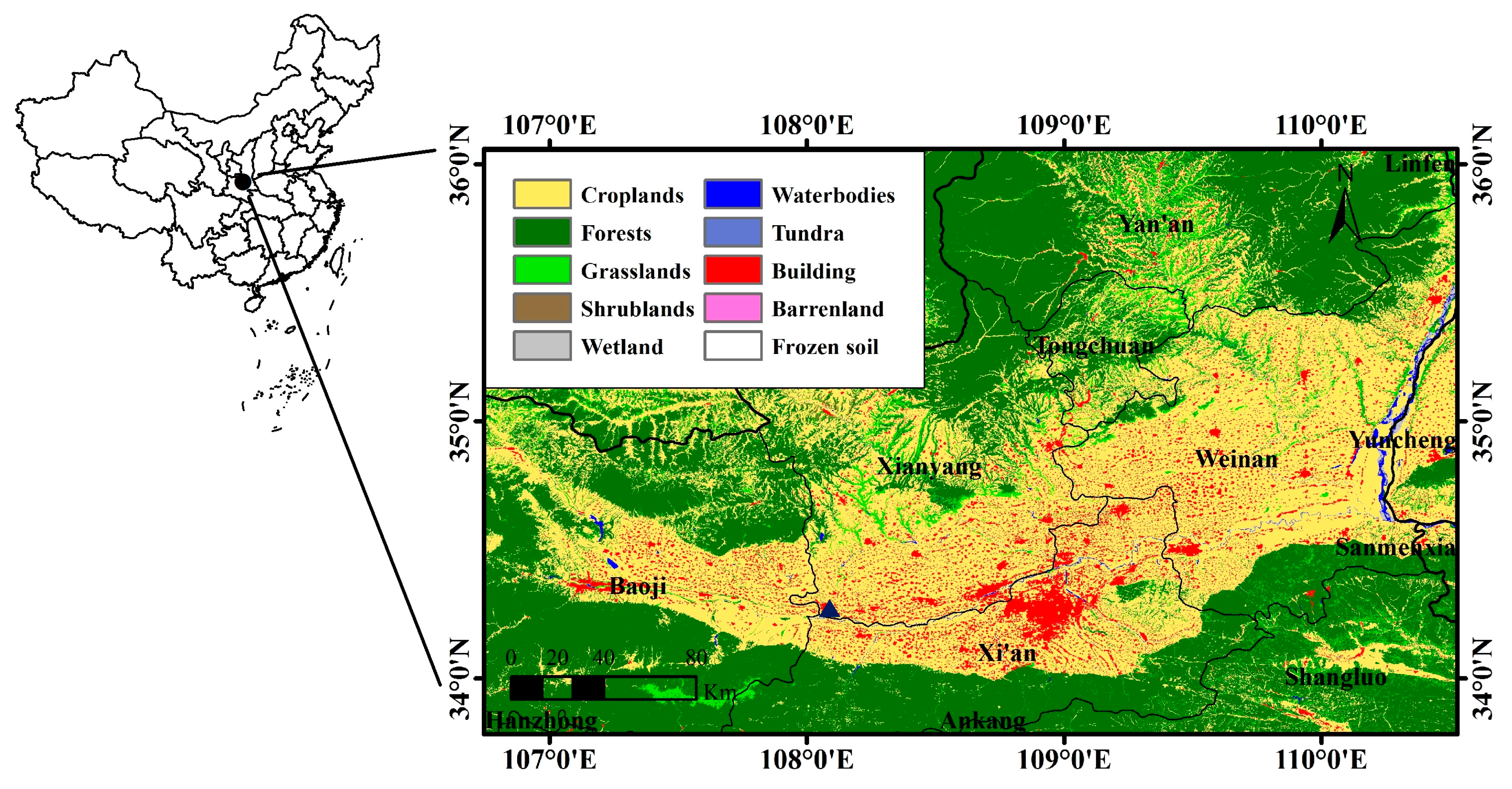
2.1. Study Area

The study was carried out in a typical irrigation agricultural district of Guanzhong Plain, Northwest of China (34°17′N, 108°04′E, 506 m a.s.l) (Figure 1). Winter wheat-summer maize rotation is a common practice of the region, dominating more than 80% of the total cropland. The region is characterized as a typical continental monsoon climate in the semiarid warm temperate zone, with average annual temperature, precipitation and potential evapotranspiration of 12.9 °C, 635.1 mm and 1500 mm, respectively. The irrigation experiment was conducted at a water-saving irrigation station operated by the Agricultural Soil and Water Engineering Laboratory. The soil at the experimental site is classified as the loamy type, with mean soil hydraulic properties in the root zone of 0–80 cm depth of field capacity of 0.31 cm³∙cm⁻³, wilting point of 0.12 cm³∙cm⁻³ and bulk density of 1.31 cm³∙cm⁻³.

2.2. Experimental Design

Nine irrigation scenarios were designed for two consecutive winter wheat growing seasons, 2013–2014 and 2014–2015. Irrigation amount (expressed in depth (mm): cubic meter per hectare) and periods, two important factors in irrigation scheduling and implementation, were considered in the experimental design. According to the seasonal water demands of the winter wheat in this region [3,4], irrigation amount was determined at two levels, 80 mm (sufficient) and 40 mm (insufficient). For each plot, irrigation was applied three times at five growing stages (with two successive stages without irrigation), resulting in eight irrigation strategies with an annual total irrigation amount of either 120 mm or 240 mm. A reference treatment with 80 mm irrigation at each stage was designed as the healthy growth condition. Each deficit irrigation scenario had three replicates, while the reference treatment only had two replicates due to restrictions of plot space. Detailed irrigation scenarios are provided in

Table 1. Winter wheat irrigation scenarios design. The capital letter “I” with a subscript number represents irrigation depth of either 80 mm or 40 mm at each growth stage; the capital letter “D” with a subscript letter represents no irrigation at these stages, and the two letters following “D” are the first letter of growth period; for instance, “D_W-R” represents no irrigation at wintering and reviving stages.

Irrigation Schedules	Irrigation Scenarios
	I40DW-R	I40DR-J	I40DJ-H	I40DH-F	I80DW-R	I80DR-J	I80DJ-H	I80DH-F	I80
Wintering	0	40	40	40	0	80	80	80	80
Reviving	0	0	40	40	0	0	80	80	80
Jointing	40	0	0	40	80	0	0	80	80
Heading	40	40	0	0	80	80	0	0	80
Filling	40	40	40	0	80	80	80	0	80
Total amount(mm)	120	120	120	120	240	240	240	240	400

.

A total of 26 plots were developed. For precise water supply control, all experimental plots were under a large mobile shelter to prevent the impact of natural precipitation. The plot size was 2 m × 4 m, with nine rows of plants. Spacing between neighboring plots was 0.4 m, and a 1.5 m deep waterproof layer was placed to prevent soil water movement between plots. The wheat was sown on 15th October 2013 and 2014, and was harvested on 7th June 2014 and 2nd June 2015, respectively. Before sowing, the 0–20 cm soil layer of all plots was manually fertilized with total N of 140 kg⋅ha⁻¹ and P₂O₅ 50 kg⋅ha⁻¹, and then the soil was smoothed and flattened for sowing. Other crop management practices were also followed to control weeds, pests, and disease.

2.3. Data Collection

2.3.1. Crop Data

Crop development was monitored regularly throughout the winter wheat growth cycle. LAI, aboveground biomass, and grain yield data were collected. LAI was measured using a SunSCAN Canopy Analysis System (Delta-T Devices Ltd., Cambridge, UK). The 64 photosynthetically active radiation (PAR) sensors of the SunSCAN were integrated into a 1-m long probe, measuring the incident and transmitted PAR to determine LAI. All measurements were carried out under cloudless condition during midday. The sensor probe was placed along the row direction in the middle of five rows of each plot. For each plot, measurements were taken as the average of three readings using a palmtop.

After the measurements of LAI, the aboveground portions of 15 randomly selected plants were removed. They were then dried in an oven at 75°C for 48 h to determine the dry biomass. The number of plants per 1 m² was counted to determine plant density. The dry biomass per unit area was calculated by multiplying dry mass per plant with the plant density. Grain was harvested within 1 m² area at full maturity stage, threshed and air-dried to constant weight to determine the final grain yield.

2.3.2. Canopy Spectral Measurements

Crop canopy reflectance spectra were measured under cloudless and windless conditions between 11:00 and 13:00 local time, using an ASD FieldSpec 3 Spectroradiometer (Analytical Spectral Device, Inc., Boulder, CO, USA). At each plot, the measurement was made at the most uniform, representative, and pest-free area. The instrument was equipped with a 25° field-of-view (FOV) fore-optics, and spectral measurements were taken at a height of 1.3 m above the top of canopy with sensor looking vertically downward, covering three rows of plants. Ten scans were made at each plot, with a reference measurement over a white panel every five minutes. The reflectance spectra were smoothed using a Savitzky-Golay filtering (with a quadratic polynomial of five spans) to reduce instrument noise.

2.3.3. Soil Moisture

Simultaneous to other measurements, soil moisture was measured using a neutron probe (Nanjing Chishun Science and Technology Co., Ltd., China), in the 0−100 cm soil profile at five layers with 20 cm interval. The actual crop evapotranspiration (ETa) was calculated using a water balance function (Equation (8)).

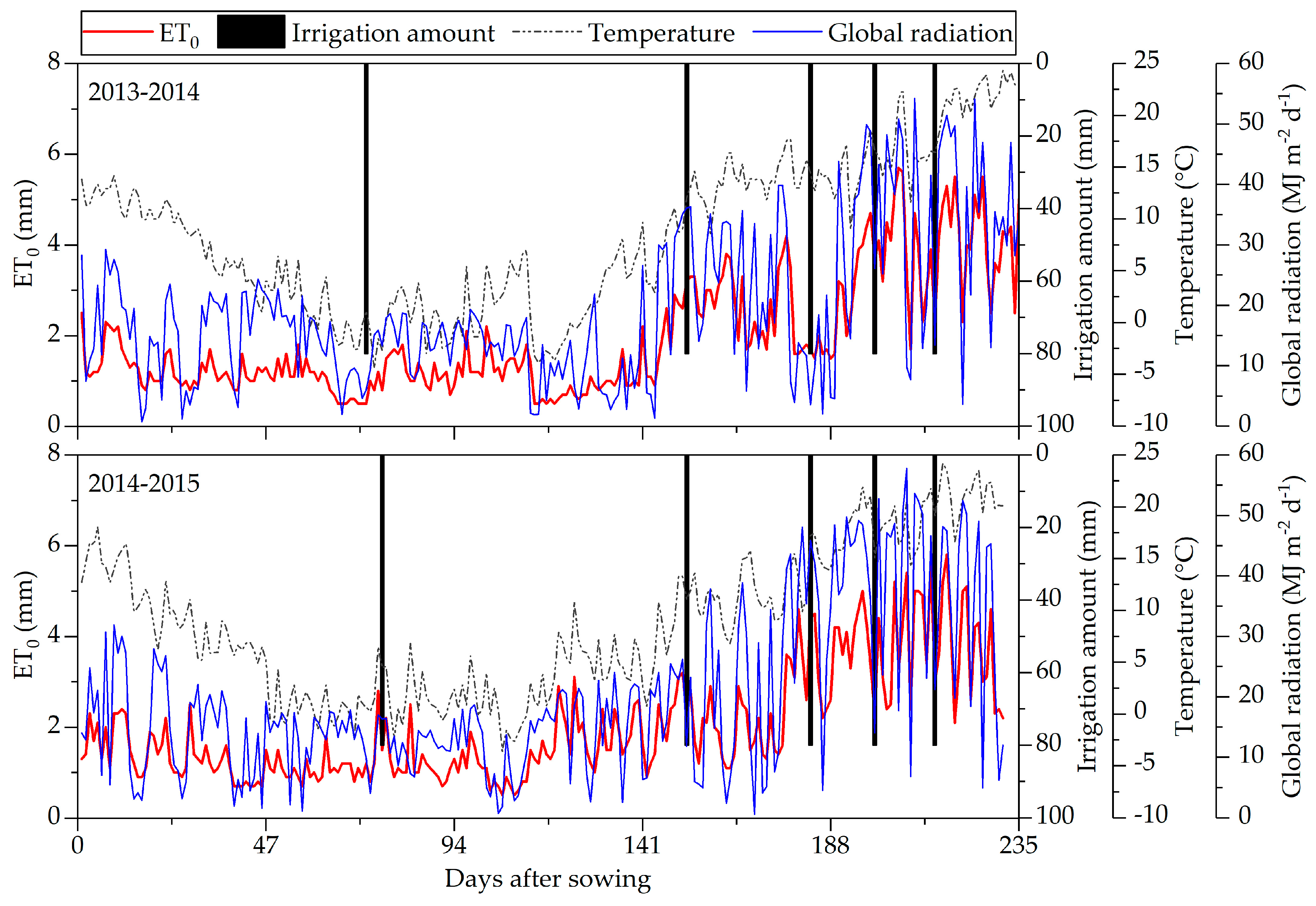
2.3.4. Meteorological Data

The meteorological data, including air temperature, solar radiation, wind speed, relative air humidity, and precipitation, were automatically collected by a Dynamet weather station (Dynamax Inc., Houston, TX, US). Air temperature and relative humidity were measured using a temperature/humidity sensor (HMP60, Campbell Scientific Inc., Logan, UT, US) at 2 m above the ground. Solar radiation was recorded with a silicon radiation sensor (LI–200SZ, Li-Cor Inc., Lincoln, NE, US). Wind speed and direction were also measured at the same height. All data was regularly logged in a data logger (CR1000, Campbell Scientific Inc., Logan, UT, US). Daily solar radiation, mean air temperature and reference evapotranspiration (ET₀) during the crop growing season are shown in Figure 2.

2.4. LAI Estimation from Canopy Spectral Reflectance

Several methods can be used to retrieve crop LAI from spectral reflectance, such as inversion from radiation transfer model, estimation using a vegetation index and non-parameter regression [27]. The partial least squares regression (PLSR), taking full advantage of spectral information, was used to retrieve crop LAI in this study. PLSR constructs several components to interpret both the independent variables of spectral reflectance and the dependent variable of LAI. In this study, the optimum number of components was determined using a 10-fold cross-validation. Detailed information on the estimation can be found in Zhang, et al. [28].

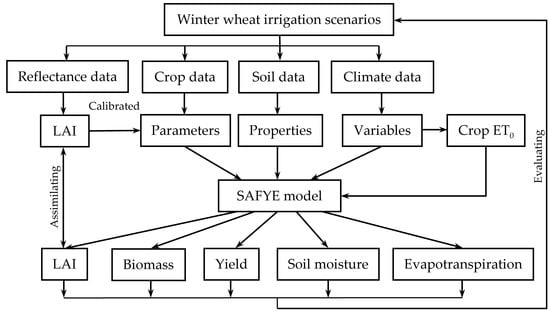
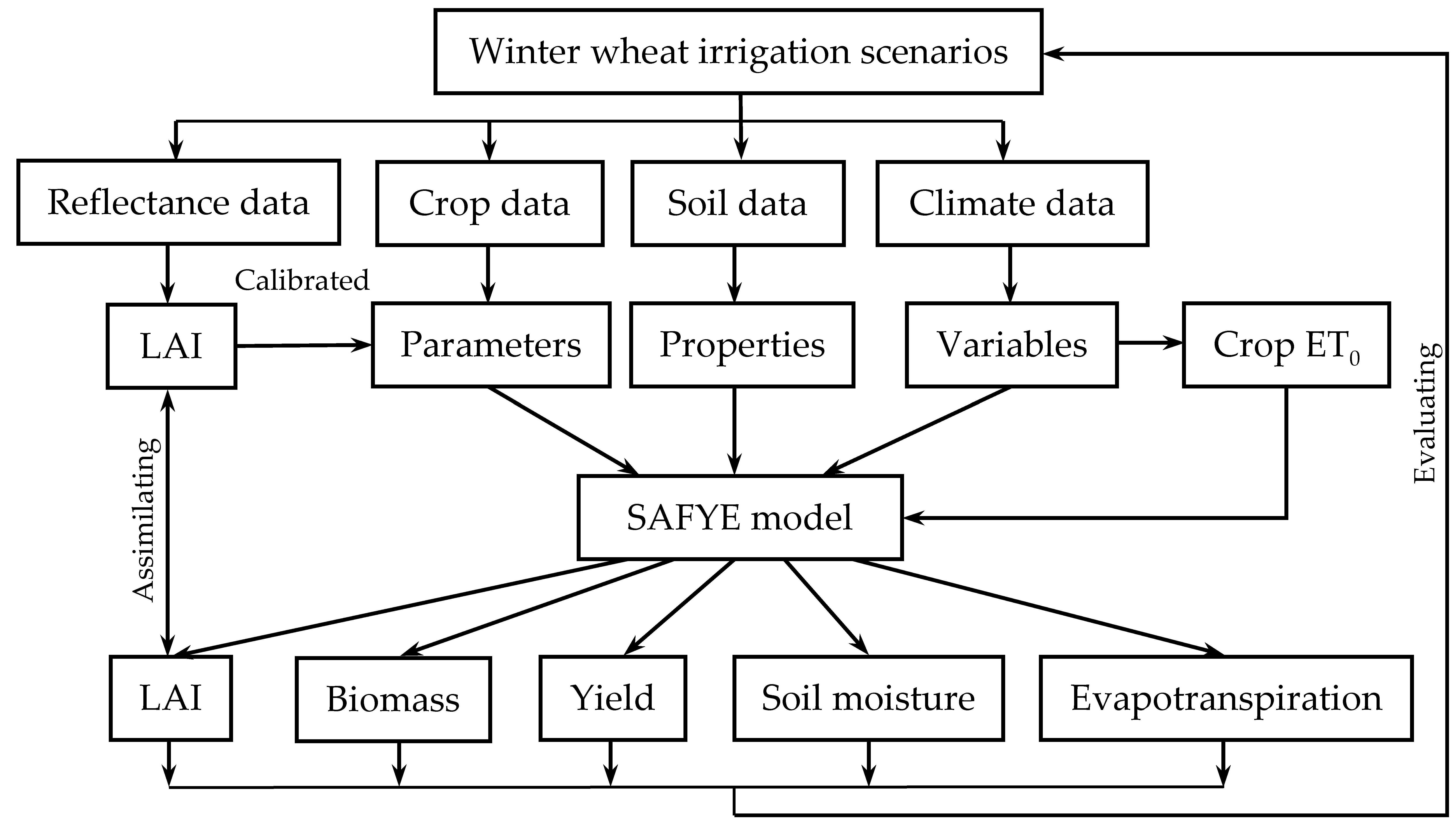
2.5. The SAFYE Model

The SAFYE model, developed by Duchemin, et al. [29] and Battude, et al. [30], was used in this study. This model couples the original SAFY crop growth model [25] with the FAO-56 soil water budget model [31] to simulate crop growth and soil moisture at a daily step, including LAI, aboveground biomass, grain yield, crop transpiration, and soil water content.

The SAFYE model simulates daily green LAI (GLAI) and biomass based on the light-use efficiency (LUE) theory [26]. The main model processes were as follow: daily aboveground matter (M_d) was accumulated as a conversion from the absorbed radiation into chemical energy, calculated as a function of LUE and absorbed photosynthetically active radiation (APAR) (Equation (1)). Besides, effects from the temperature (Ft) and soil water (Ks) on LUE were also considered:

$$\Delta {\mathrm{M}}_{\mathrm{d}}=\mathrm{APAR}\times \mathrm{LUE}\times {\mathrm{F}}_{\mathrm{T}}\times {\mathrm{K}}_{\mathrm{S}}$$

(1)

The APAR was calculated from LAI and solar radiation (R_g) using the Beer-Lambert function [32] (Equation (2)). The function parameters ε_c and k were climatic efficiency factor (~0.48) and the light extinction coefficient of canopy, respectively.

$$\mathrm{APAR}={\mathsf{\epsilon }}_{\mathrm{c}}\times {\mathrm{R}}_{\mathrm{g}}\times \left(1-{\mathrm{e}}^{-\mathrm{k}\times \mathrm{LAI}}\right)$$

(2)

The F_T is a temperature stress factor, which can be calculated by a quadratic polynomial function derived from the STICS model [33]. The K_S is water stress factor, calculated as a function of soil moisture. Battude et al. [30] assumed a linear function for crop water stress in SAFYE. Considering that the drought tolerance of wheat is not sensitive to mild water stress condition, a nonlinear stress coefficient of K_S was incorporated to the SAFYE model in this study. Specifically, a convex stress response function was used following the AquaCrop model [34,35] (Equation (3). The value of K_S varied between 1 (no stress) to 0 (full stress) and was determined by a curve shape factor of f and relative depletion of soil moisture of S_rel.

$${\mathrm{K}}_{\mathrm{s}}=1-\frac{{\mathrm{e}}^{{\mathrm{S}}_{\mathrm{rel}}\mathrm{f}}-1}{{\mathrm{e}}^{\mathrm{f}}-1}$$

(3)

The S_rel, defined as the relative depletion of soil moisture, was calculated by the ratio of root depth layer soil moisture (SM_r, mm) to total available moisture (TAW, mm) (Equation (4)). Crop water stress would not develop immediately following the start of soil moisture relative depletion. The range of water stress was constraint by two parameters, upper (P_u) and lower (P_l) threshold limits, which means that plants will be subject to water stress when relative water depletion is less than P_u and becomes fully stressed when depletion is less than or equal to P_l.

$${\mathrm{S}}_{\mathrm{rel}}=\{\begin{array}{cccc}\hfill 1,& & & {\mathrm{p}}_{\mathrm{u}}\le {\mathrm{S}}_{\mathrm{rel}}\hfill \\ \hfill \frac{{\mathrm{p}}_{\mathrm{u}}-\frac{{\mathrm{SM}}_{\mathrm{r}}}{\mathrm{TAW}}}{{\mathrm{p}}_{\mathrm{u}}-{\mathrm{p}}_{\mathrm{l}}},& & & {\mathrm{p}}_{\mathrm{l}}<{\mathrm{S}}_{\mathrm{rel}}<{\mathrm{p}}_{\mathrm{u}}\hfill \\ \hfill 0,& & & {\mathrm{S}}_{\mathrm{rel}}\le {\mathrm{p}}_{\mathrm{l}}\hfill \end{array}$$

(4)

The daily LAI variation includes increase with leaf generation and decrease with leaf senescence. Daily new LAI at the vegetative stage is determined based on the biomass partitioning concept (Equation (5)). The LAI decrease at senescence stage is calculated when the accumulated temperature (AT, (°C)) reaches threshold parameter (S_TT, (°C)), and the decreasing ratio is decided by parameter Rs (°C·d⁻¹) (Equation (6)). The leaf partitioning at the reproductive stage is driven by two temperature parameters, Pl_a and Pl_b (Equation (7)).

$$\Delta {\mathrm{LAI}}^{+}=\Delta {\mathrm{M}}_{\mathrm{S},\mathrm{d}}\times \mathrm{Pl}\times \mathrm{SLA}$$

(5)

$$\Delta {\mathrm{LAI}}^{-}={\mathrm{LAI}}_{\mathrm{t}-1}\times \frac{\left(\mathrm{AT}-{\mathrm{S}}_{\mathrm{TT}}\right)}{{\mathrm{R}}_{\mathrm{s}}}$$

(6)

$$\mathrm{Pl}=1-{\mathrm{Pl}}_{\mathrm{a}}{\mathrm{e}}^{{\mathrm{Pl}}_{\mathrm{b}}\times \mathrm{AT}}$$

(7)

For soil water balance, water transport among soil, plant and atmosphere in SAFYE’s water balance module was determined by water budget equation (Equation (8)):

$$\Delta \mathrm{SW}=\mathrm{P}+\mathrm{I}+\mathrm{GF}-\mathrm{ET}-\mathrm{SR}-\mathrm{DP}$$

(8)

where P, I, GF, ET, SR and DP represent precipitation, irrigation, groundwater flow, evapotranspiration, runoff, and deep percolation, respectively. SAFYE simplifies the water transfer processes in three soil layers (evaporation layer, root layer, and deep layer). The daily change of soil water storage was calculated from different water inflow and outflow sources.

Evapotranspiration is the most important component in soil water consumption, consuming almost all water storage in root zone. Crop actual evapotranspiration (ETa) is calculated using the FAO-56 dual crop coefficient model, which consists of a crop transpiration component and a soil evaporation component [31]. The crop water stress is described by multiplying the basal crop coefficient with the water stress coefficient of K_s (Equation (9)).

$${\mathrm{ET}}_{\mathrm{a}}=\left({\mathrm{K}}_{\mathrm{e}}+{\mathrm{K}}_{\mathrm{cb}}\times {\mathrm{K}}_{\mathrm{s}}\right)\times {\mathrm{ET}}_0$$

(9)

Soil water evaporation mainly happens in topsoil and is impacted by crop canopy cover. Soil evaporation coefficient K_e is calculated using a semi-empirical equation based on evaporation reduction coefficient (β) and relative depletion soil moisture in top of 0–20 cm soil layer (RSM) [30,31] (Equation (10)):

$${\mathrm{K}}_{\mathrm{e}}=\left(1-\mathrm{CC}\right)\times [1-{\left(1-\mathrm{RSM}\right)}^{\mathsf{\beta }}]$$

(10)

where CC is canopy cover, calculated from crop LAI using a function given by Nielsen et al. [36] (Equation (11)):

$$\mathrm{CC}=94.00{\left(1-{\mathrm{e}}^{-0.43\times \mathrm{LAI}}\right)}^{0.52}$$

(11)

The basal crop coefficient K_cb represents crop potential transpiration rate when soil is dry in the top layer while moisture is sufficient in the root zone so that the crop does not experience water stress. The value of K_cb is considered to be corrected by wind speed, relative humidity and plant height in FAO 56 method. However, this method is not suitable for operational applications as many of these parameters are unavailable at regional scale. In this study, a semi-empirical equation was used to estimate K_cb from LAI (Equation (12)) [37]:

$${\mathrm{K}}_{\mathrm{cb}}={\mathrm{K}}_{\mathrm{cb},\max }\left(1-{\mathrm{e}}^{{\mathrm{K}}_{\mathrm{trp}}\times \mathrm{LAI}}\right)$$

(12)

2.6. Calibration of SAFYE Parameters

The common input variables (

Table 2. Main inputs, outputs, and parameters used in SAFYE model for calibrating and simulating winter wheat during 2013/2014 and 2013/2015 growing seasons.

	Notation	Description	Unit	Value	Sources
Inputs	Rg	Daily incoming global radiation	MJ m−2 ∙d−1
	Ta	Daily mean air temperature	°C
	P	Daily precipitation	mm
	ET0	Daily reference evapotranspiration	mm
	SM0	Initial soil moisture	m3∙m−3
Parameters	εc	Climatic efficiency	-	0.48	L
	Md0	Initial dry aboveground biomass	g∙m−2	5.3	D
	k	Light extinction coefficient	-	0.53	M
	Tmin,opt,max	Temperature for growth	°C	0,18,26	L
	SLA	Specific leaf area	m2∙g−1	0.019	M
	D0	Day of plant emergence	day	10	M
	Pla	Partition-to-leaf function: par a	-	0.589	C
	Plb	Partition-to-leaf function: par b	-	0.00023	C
	STT	Sum of temperature for senescence	°C	963	C
	Rs	Rate of senescence	°C∙d−1	14937	C
	LUE	Light-use efficiency	g∙MJ−1	2.0	L
	θFC	Field capacity	m3∙m−3	0.31	M
	θWP	Wilting Point	m3∙m−3	0.12	M
	Kcb,max	Maximum crop basal coefficient	-	1.07	L
	Ktrp	Coefficient between LAI and Kcb	-	0.84	L
	Kz	Root growth rate	m °C∙d−1	0.0009	L
	pu,pl	thresholds of soil water depletion	-	0.3, 0.65	L
	f	Water stress function curve shape	-	3	L
	β	Evaporative reduction coefficient	-	0.94	L
	HI	Harvest index	-	0.34	M
Outputs	LAI	Daily leaf area index	m2∙m−2
	Md	Daily dry aboveground biomass	g∙m−2
	Yield	Grain yield	g∙m−2
	SM	Daily soil moisture	m3∙m−3
	ETa	Crop evapotranspiration	mm

D—Default, C—Calibrated, M—Measured, L—Literature.

) for crop growth modeling are daily average temperature (T_a), incoming global radiation (R_g), precipitation (P), reference evapotranspiration (ET₀), irrigation (I), and initial soil moisture content (SM₀). The reference ET₀ was derived from meteorological data (e.g., air temperature, humidity, radiation) using the FAO Penman-Monteith method [31] (http://www.fao.org/).

Other parameters in SAFYE (Table 2) require careful calibration before model simulation. The parameters in the crop model can be classified into two categories, conservative and specific. The conservative parameters are general to a given species, without significant change in most cases. They can be obtained from prior knowledge or literatures. Such parameters include ε_c, T_min,opt,max, K_cb,max etc. The ε_c was usually a constant, and the value was fixed to 0.48 [38]. Daily mean temperature is used in SAFYE to restrict or promote crop growth. The optimal temperature for wheat growth is about 18°C, and the range of temperatures for wheat to grow is from 0°C (T_min) to 26°C (T_max) [39]. The parameters K_cb,max and K_trp were determined as 1.07 and 0.84 [37], as recommended in FAO-56 documentation [31]. The values of p_u, p_l and f were fixed to 0.3, 0.65 and 3, assuming a moderate water tolerance [40,41]. The general root expansion rate (K_z) of wheat is about 0.8–1.2 mm·d⁻¹°C⁻¹ [33], and was set to 0.9 mm·d⁻¹°C⁻¹ in this study [42]. Theoretically, LUE is almost constant for a given crop, but could vary in different natural ecosystems and cultivars. Most studies reported that LUE of wheat was about 2.0–2.2 g·MJ⁻¹ [43,44,45]. The LUE was assumed to be a constant and was set to 2.0 g·MJ⁻¹ in this study. Other parameters in SAFYE could be calibrated using in situ measurement, such as k, SLA, and HI. The parameters of k, SLA and HI were calibrated to 0.53, 0.019 and 0.34 using in situ data. The main parameters are presented in Table 2.

Non-conservative parameters need to be adjusted by cultivar, environment and management practices. As referred to in the section, crop growth is mainly determined by four parameters (Pl_a, Pl_b, S_TT and R_s), which were optimized in this study. The data assimilation approach was adopted in this study for parameter calibration, by minimizing the difference between simulated time-series LAI and the measured or estimated LAI from canopy reflectance. The Root Mean Square Error (RMSE) was used as the merit function for data assimilation and parameter calibration (Equation (13)):

$$\min \to \mathrm{RMSE}=\sqrt{\frac{1}{\mathrm{n}}{\displaystyle \sum _{\mathrm{i}=1}^{\mathrm{n}}}{\left({\mathrm{LAI}}_{\mathrm{obs}}-{\mathrm{LAI}}_{\mathrm{sim}}\right)}^2}$$

(13)

where LAI_obs,i and LAI_sim,i are the retrieved and simulated LAI, respectively. n is the numbers of observations for a plot during a growing season.

The SCE-UA (Shuffled complex evolution method developed by Duan, et al. [46] was used in this study for the optimization process. Compared to other optimization algorithms (e.g., PSO and GA), the concept of competitive and shuffled complex evloution used in the method is not sensitive to the initial values of the parameters, which could prevent convergence to a local opmimal solution [47,48]. Setting reasonable variation ranges for the parameters can improve the efficiency of optimization. The ranges of the four parameters (Pl_a, Pl_b, S_TT, and R_s) were determined as: Pl_a [0.1–0.7], Pl_b [0.0001–0.001], S_TT [500–1600] and R_s [5000–20000] according to previous studies [46,49]. The model was calibrated using the data of unstressed healthy plots (I₈₀) during the 2013–2014 growing season. To reduce the uncertainty due to the unique solution in one optimization process, 1000 repetitions were conducted and the median value of the frequency for each parameter optimal solution was selected. The values of the four parameters optimization are presented in Table 2.

After the calibration procedure, all parameters were fixed and the model was applied to simulate LAI, biomass, ETa and water balance under different irrigation scenarios in the two growing seasons. The grain yield was determined by multiplying the total aboveground biomass at full maturity with the harvest index (HI). The estimated LAI, biomass, ETa and soil moisture were evaluated against field measurement data. Several statistical criteria including coefficient of determination (R²), RMSE, relative RMSE (RRMSE), relative error (RE) and mean relative error (MRE) were used to evaluate the performance of the model corresponding to different water stress condition.

3. Results

3.1. Accuracy of LAI Estimation from Spectral Reflectance Data

Comparisons between in situ measured and estimated LAI from spectral reflectance using the PLSR method are shown in Figure 3. The results show good estimation accuracy with a R² of 0.89 and RMSE of 0.42 m²∙m⁻². We thus considered that the retrieved LAI was acceptable for assimilating into the SAFYE model.

3.2. Evaluation of the SAFYE Model Simulation

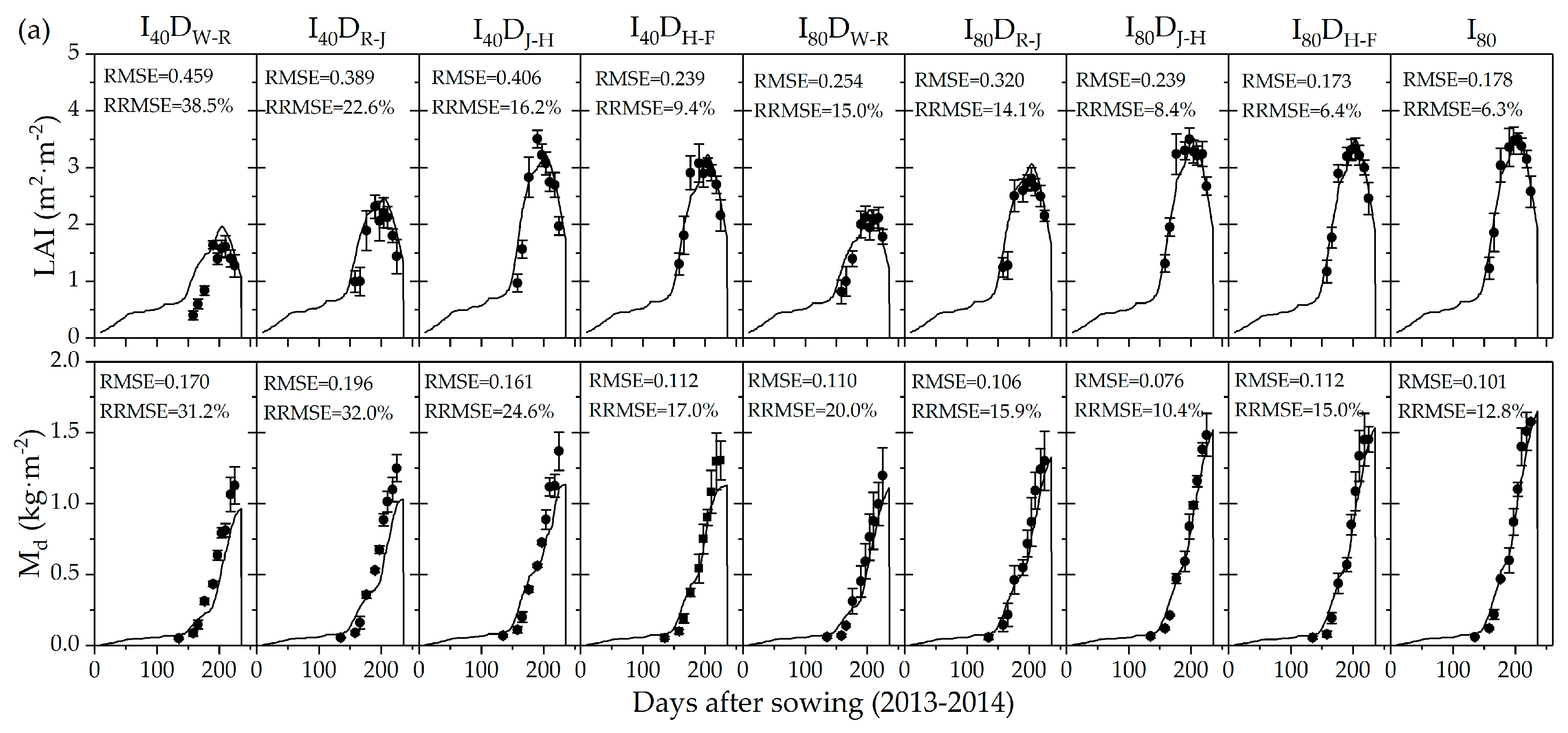
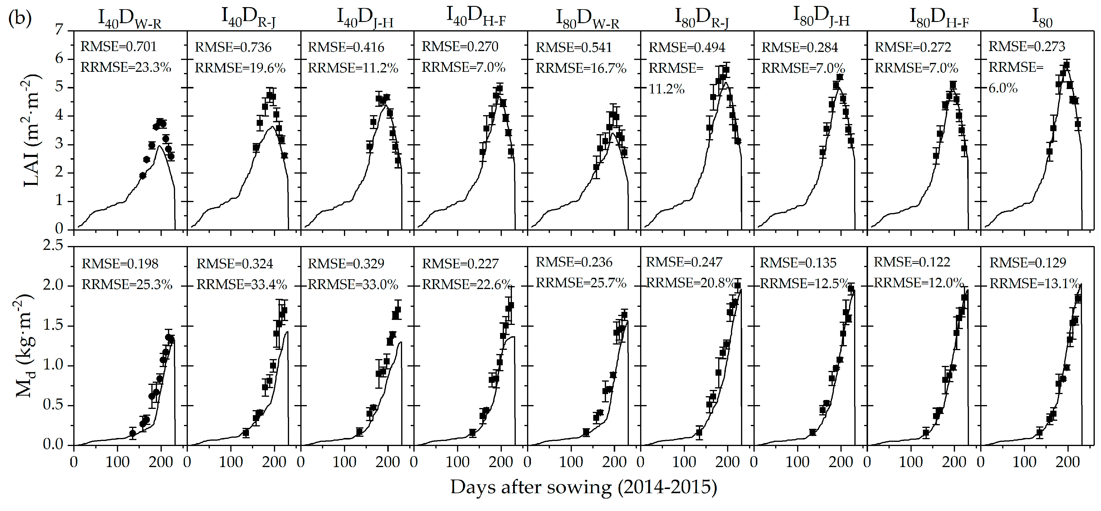
3.2.1. Leaf Area Index

A comparison between the simulated and retrieved LAI for the nine irrigation scenarios through the two growing seasons is shown in Figure 4. The simulated LAI had good agreement with estimated LAI for most of the irrigation scenarios, with a minimum error of 0.173 m²∙m⁻². Results showed that all five irrigation scenarios of 80 mm irrigation amount had a higher accuracy (RMSE: 0.173–0.320, 2013–2014; RMSE: 0.272–0.541, 2014–2015) than those of 40 mm irrigation amount (RMSE: 0.239–0.459, 2013–2014; RMSE: 0.270–0.736, 2014–2015) in both growing seasons. For both irrigation levels (40 mm or 80 mm) in both years, simulation accuracy in the later stages of water deficit scenarios (D_J-H, D_H-F) was better than that of the early stages (D_W-R, D_R-J).The accuracy, assessed using RRMSE as the global simulation accuracy, is considered to be excellent when RRMSE<10%, good when 10%< RRMSE <20%, fair when 20% < RRMSE <30%, and poor if the RRMSE is >30% [50]. Excellent accuracy was achieved in late deficit stages (e.g., I₈₀D_J-H and I₈₀D_H-F), and fair or even poor in I₄₀D_W-R and I₄₀D_R-J. However, the inconsistent results were also presented in scenarios D_W-R and D_R-J, with the overestimation of LAI in 2013–2014 and underestimation in 2014–2015. Therefore, the performance of the model for responding early water deficit and later re-irrigated scenarios were imperfect.

3.2.2. Aboveground Biomass

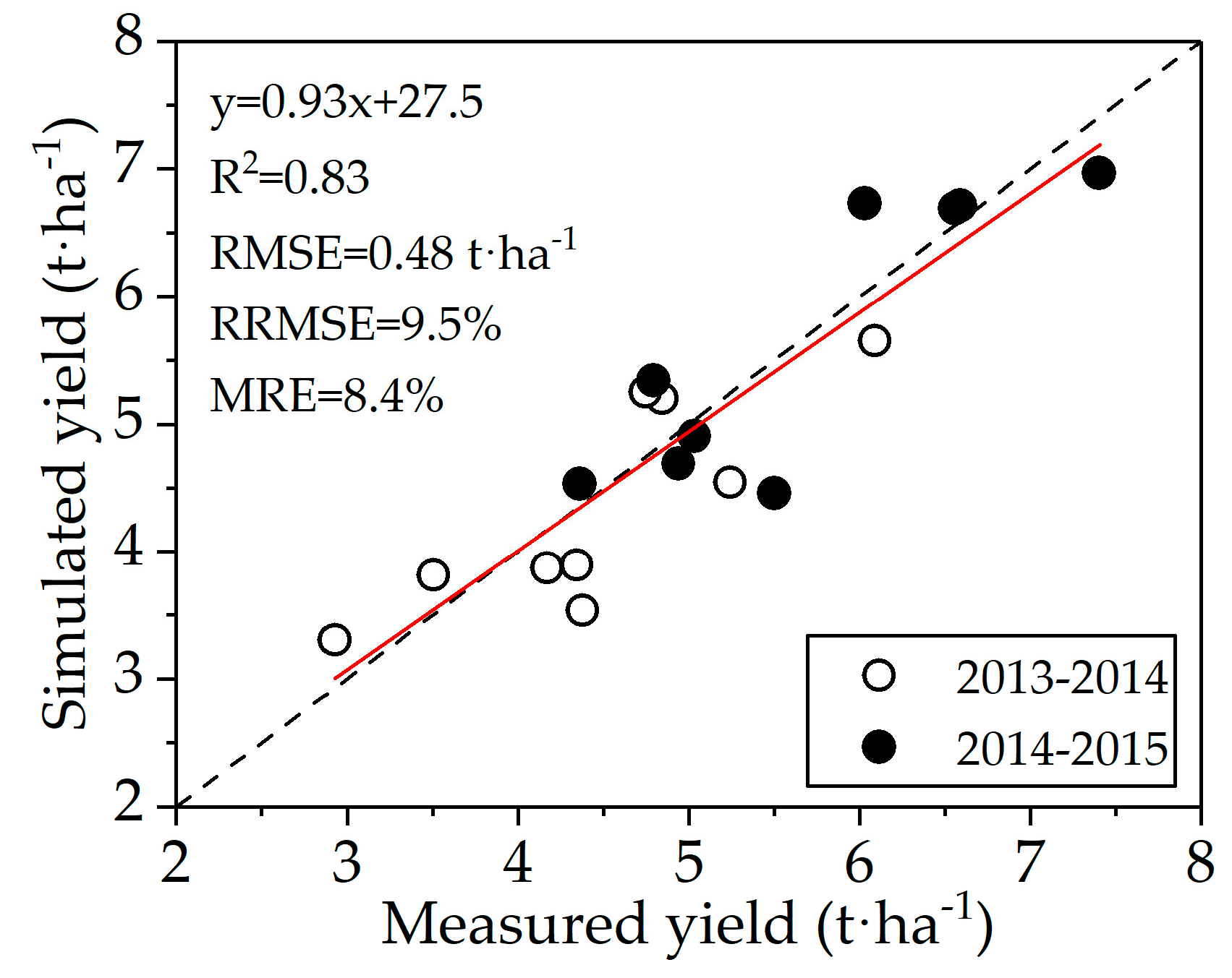
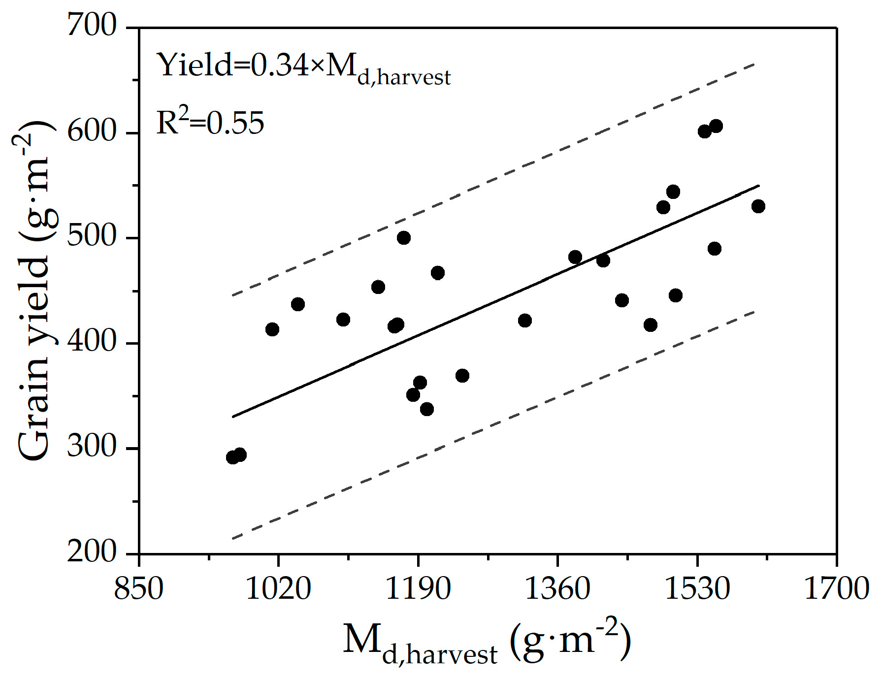
The seasonal dynamics of the simulated dry matter was consistent with in situ measured dry matter in both growing seasons (Figure 4). The performance was similar to that of LAI, with an acceptable agreement in late water deficit stages and relatively large discrepancy in the early stages. Results revealed that simulation accuracy increased with delayed water deficit stage for both seasons. Obvious underestimation were observed for both growing seasons for the treatments of 40 mm irrigation depth (I₄₀D_W-R, I₄₀D_R-J, I₄₀D_J-H and I₄₀D_H-F), with the maximum RRMSE reaching 33%. Large deviation appeared from 180 days after sowing and continuously expended to maximum at the end of stage.

3.2.3. Grain Yield

Winter wheat grain yield was calculated by multiplying the final aboveground plant dry matter a HI. A mean value was used for HI and was derived from a global regression analysis of the field data (Figure 5). The ratio of grain yield to final aboveground ranged was from 0.28 to 0.43 for all irrigation scenarios, and the regression coefficient for all the samples was 0.34. The regression coefficient is within the ranges of HI found in literatures [51,52]. The grain yield simulation of the remaining plots showed a good agreement with in situ measured yield for all irrigation scenarios (R^{2 =} 0.83; RMSE = 0.48 t∙ha⁻¹; RRMSE = 9.5%; MRE = 8.4%) (Figure 6). Grain yield in 2015 was higher than that in 2014 due to comparatively more favorable meteorological conditions and initial soil moisture. As aforementioned, the values of simulated M_d were generally lower than that of measured M_d in field of 40 mm irrigation scenarios, while the results of grain yield were all close to the 1:1 line, suggesting that the actual HI was close to that obtained through regression analysis (0.34).

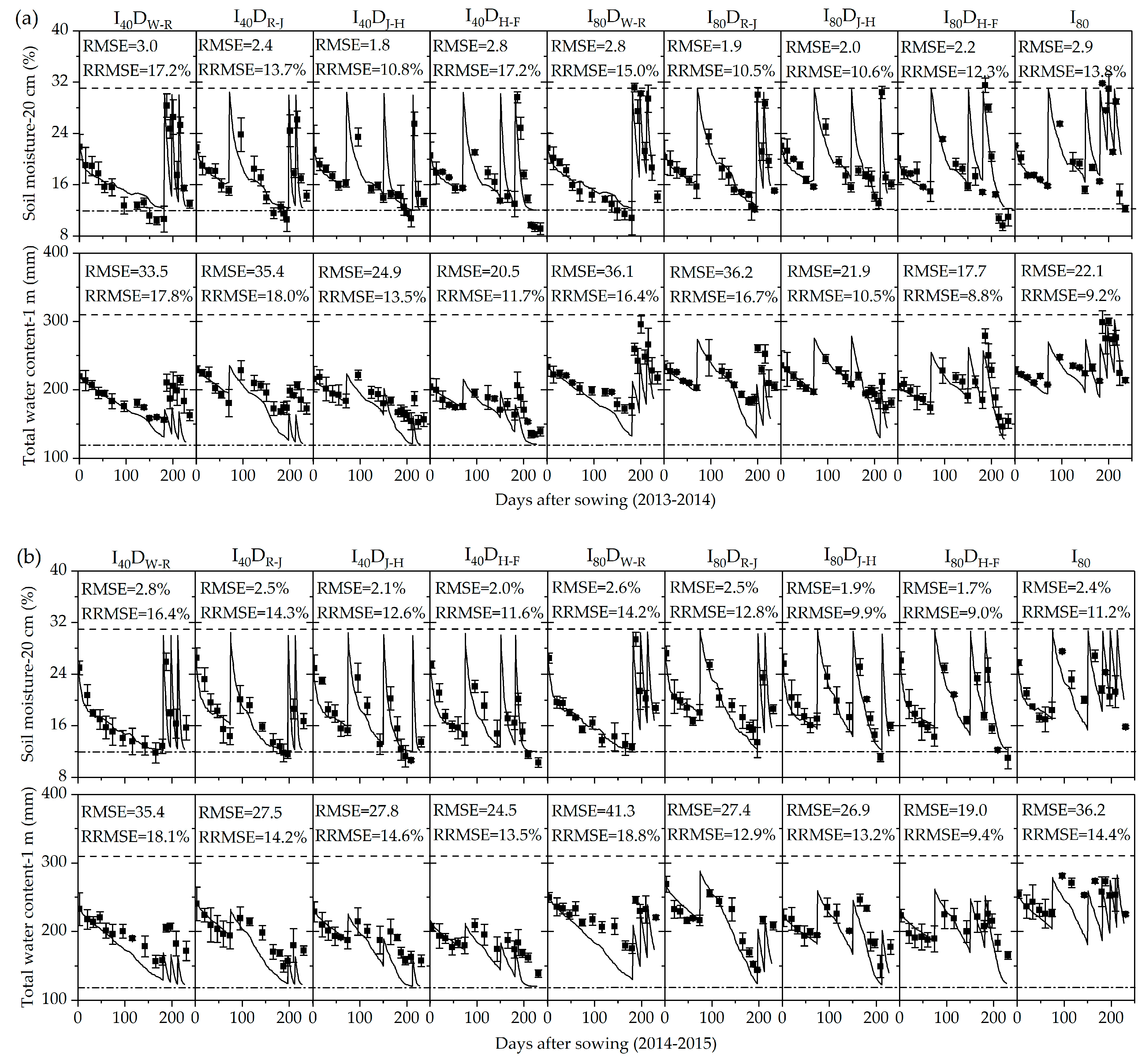
3.2.4. Soil Moisture

Soil moisture simulations for the top 0.2 m and 1 m soil layers were quantitatively evaluated against the in situ measured data (Figure 7). For the top 0.2 m soil layer, dynamics of the simulated soil moisture follow the variation of the measured moisture consistently for all irrigation scenarios in the two growing seasons, with the maximum and minimum RMSE of 3% and 1.8% in 2014 and 2.8% and 1.7% in 2015 respectively. The simulation performance was comparable for 40 mm and 80 mm irrigation levels. Discrepancies of soil moisture simulation mainly exist in long-term water deficit and rapid declining stages after irrigation. The assumption of the water balance model is that, soil moisture cannot exceed field capacity and fall below permanent wilting point.

For the root zone, the SAFYE model could simulate the soil moisture reasonably well in the early stage. However, with increasing root depth (about 100 days after sowing), the difference between the simulated and measured moisture increased (Figure 7). In general, the simulated total soil water content followed the trend of the actual measured values, although a general tendency of underestimation was observed after about 100 days from sowing, when the winter wheat was at the dormancy stage. The rapid decrease in soil moisture storage indicated that soil moisture was consumed to supply crop growth, reflecting the continuous rise of LAI and dry matter (Figure 4). During the later stage (about 200 days after sowing), the difference between simulated and measured soil moisture increased gradually due to the cumulative deviation from the early stages. The relatively higher simulation errors were observed under early water deficit scenarios (e. g., I_40/80D_W-R) than that in other scenarios. This suggests that, although the crop water stress module was optimized using a nonlinear function, variation of soil moisture with crop development cannot be adequately simulated.

3.2.5. Crop Evapotranspiration

Crop evapotranspiration plays an essential role in the soil-plant-atmosphere system. Timely and accurate estimation of evapotranspiration is important for determining crop water demand and regulating irrigation schedules.

Table 3. Statistics of simulated and measured actual evapotranspiration (ETa) for winter wheat in two consecutive growing seasons. The RE represented the relative error.

Irrigation Scenarios	2013–2014			2014–2015
	ETa (mm)			ETa (mm)
	Obs.	Sim.	RE (%)	Obs.	Sim.	RE (%)
I40DW-R	177	218	23.5	181	233	28.6
I40DR-J	177	230	29.6	188	243	29.1
I40DJ-H	179	215	20.0	191	233	21.8
I40DH-F	185	205	10.3	188	217	15.5
I80DW-R	256	297	16.0	263	316	19.8
I80DR-J	268	329	23.1	301	356	18.5
I80DJ-H	294	344	17.0	282	329	16.4
I80DH-F	291	321	10.3	298	349	17.1
I80	414	421	1.5	429	453	5.5

shows the simulation results of the actual evapotranspiration (ETa) during the entire winter wheat growing period. In general, the dynamics of the simulated ETa fits well with the measured ETa (R² = 0.97, RMSE = 43.4 mm, MRE = 17.9%), although with an overestimation.

The simulated ETa was about the same for the two growing seasons for all irrigation scenarios, ranging from 205 to 421 mm in the 2013–2014 growing season and from 217 to 453 mm in the 2014–2015 growing season. The overestimation was more than 10% for most irrigation scenarios except for the sufficient irrigation treatments (I₈₀). The maximum and minimum relative error were 29.1% and 29.1% for I₄₀D_R-J and 1.5% and 5.5% for I₈₀ in both seasons, respectively. The simulation confirmed the previous results that, excessive soil moisture was consumed for maintaining crop growth; from which, the general overestimation of ETa for all scenarios was observed. The results suggest that the model had produced a higher accuracy in estimating crop ETa for mild water stress conditions (total 240 mm irrigation depth) and crop water consumption in later period of water deficit scenarios (D_H-F).

4. Discussion

Increased model complexity does not necessarily increase model robustness [53,54]. The SAFYE model was designed to simulate crop growth and water demand using a series of simple procedures, which are suitable for regional-scale applications or under unknown initial conditions.

Model calibration is an essential process leading to successful model applications. In contrast to most model calibrations using field measured data, this study conducted model calibration through assimilation of remotely sensed crop variables (e.g., LAI, canopy cover and biomass) into a crop model. Remote sensing data provides a means for acquiring spatial-temporal information of crop variables. Crop LAI, the most commonly used indicator in both agronomy and geoscience, was used as state variable assimilated into the SAFYE model in this study to calibrate four main parameters, Pl_a, Pl_b, S_TT, and R_s that control crop growth and senescence processes. These parameters were calibrated based on a typical condition (e.g., sufficient irrigation scenarios (I₈₀)) and remain unchanged and then applied to other scenarios using stress coefficients (e.g., K_s). Different calibration strategies can be found in literature. For instance, Claverie, et al. [38] and Dong, et al. [16] considered that parameters were crop specific for which statistical analysis can be adopted for calibration. Battude, et al. [55] pointed out that calibration needs to be conducted at the field level because variability such as crop species or management practices (e.g., plant seeding date) might be field specific.

The simulated LAI showed good accuracy for sufficient irrigation and moderate deficit irrigation scenarios in both growing seasons (Figure 4), whereas the accuracy was low for severe water deficit scenarios (I₄₀), with greater uncertainty especially at the early stages of water deficit scenarios (D_W-R and D_R-J). The consistent results on biomass simulation in both seasons showed good agreement at 80 mm irrigation level. Obvious underestimations appeared at 40 mm irrigation level, reflecting intense water stress response especially during the later stages. Temperature stress (F_T) and water stress (K_s) are the two main down regulating factors to crop biomass accumulation (Equation (1)). Underestimation of dry matter could be attributed to inadequate modeling of these stress factors.

Figure 8 depicts the seasonal variation of water stress coefficient. Large differences of crop stress were observed between 40 and 80 mm irrigation treatments. Under early deficit scenarios (D_W-R), long-term water stress at 170 days result in a Ks lower than 0.2. The discrepancies increased during the later stages, with frequent stresses under 40 mm scenarios and with almost no stress under 80 mm scenarios. Winter irrigation could delay potential stress period and reduce the level of stress level. Although the nonlinear stress equation was integrated into the model to optimize stress estimation in the water balance module, biomass accumulation of the 40 mm irrigation scenarios at the later stage was impacted by severe water stress, resulting in an underestimation. Throughout the crop growing season, the threshold of water stress changes with varying water demands at different growth stages and are influenced by meteorological conditions as well [56]. This is a promising way to adjust the stress threshold at different phenological phases.

The performance of the SAFYE model was satisfactory for simulating winter wheat growth and productivity in most cases using a series of simple nodules. It has the same challenges as some complex models developed for irrigation scheduling [57] in simulating crop growth under drought conditions. Results from this study confirmed the point suggested by Claverie et al. [38] the original SAFY model, which is not sufficient in most cases of severe water deficits even with the stress functions integrated. Although underestimation of dry aboveground matter happens under some scenarios, the comparison between observed and estimated grain yield showed very good performance (R^{2 =} 0.83; RMSE = 0.48 t∙ha⁻¹; MRE = 8.4%), likely due to the compensation effects of HI (Figure 5 and Figure 6). Theoretically, the harvest index is not just a coefficient that representing efficiency from biomass to grain yield but is built from flowering stage to maturity. The change of HI is a complex process; it could rise or fall depending on severity of the level of stress, the duration and the combined environment of crop production [34]. Taking a complex model of AquaCrop as an example, the HI is divided into reference harvest index (HI₀) for non-stressed condition and an adjustment factor for interpreting the effect of water stress, heat stress, even cold stress. The daily increase of HI is assumed obeying a logistic function. The adjustment factor can be positive (water stress before yield formation) and negative (water stress affecting stomata closure and pollination). Steduto, et al. [58] suggested that HI could decline to as low as 0.2–0.3 when water stress occurred after the flowering stage or mismatched with the production environment. Therefore, several modules and tens of parameters integrated to reveal HI could lead to a significant reduction in the feasibility of the assimilation systems.

In this study, variations of soil moisture and crop water consumption were simulated using the SAFYE model with a non-linear water stress function. The convex function fits the response of winter wheat crop to water stresses nicely. Most of the discrepancies were observed when soil moisture changed suddenly after irrigation because of rapid water infiltration to deeper soil layers (Figure 7). At the root zone, however, large underestimations were observed when simulating total available water content (Figure 7). This underestimation corresponds to a global overestimation of the ETa (Table 3). This finding is in agreement with what has been reported by Duchemin et al. [29], who observed a 20% error in ETa model simulation compared to the measurements by eddy covariance. The overestimation of water demands provide false information to decision maker for more irrigation than actually needed.

5. Conclusions

This study investigated the use of SAFYE model to simulate winter wheat growth and estimate crop water demands through a data assimilation approach.

Crop leaf area index (LAI) could be accurately retrieved from canopy spectral reflectance data using a partial least square regression method (PLSR). The SAFYE model can be well calibrated by assimilating the retrieved LAI for winter wheat growth simulation under different irrigation scenarios. The calibrated model can well capture crop growth (LAI) in most cases, but showed elevated uncertainty in early water deficit scenarios, especially when using half irrigation amount (I₄₀) where crop is subjected to more severe water stress.

The simulation of time-series of aboveground biomass exhibits a consistent trend, showing good performance for mild water stress scenarios. A general overestimation occurs for severe water deficit scenarios (total 120 mm) 180 days after sowing. Despite overestimation for some irrigation scenarios, results of the final simulated grain yield were in good agreement with observation for all irrigation scenarios (R² = 0.83; RMSE = 0.48 t∙ha⁻¹; MRE = 8.4%) for both years. With respect to water consumption, the model had a good adaptability for simulating the dynamics of soil moisture at the top 20 cm layer for all irrigation scenarios. Most simulation errors occurred when soil moisture was below wilting point or at the maturity phenological stage. The general underestimations of the total water content in 1 m soil depth were observed after 100 days when winter wheat began to tiller, suggesting that the water demands for crop growth and productivity were overestimated. Such results were consistent with the comparison in crop actual evapotranspiration (ETa) that estimated ETa were over than in situ measured except for sufficient irrigation scenarios (I₈₀).

This study demonstrates that high potential of the SAFYE model for monitoring crop growth and estimating productivity and water consumption under different irrigation scenarios when with the aid of remote sensing data assimilation. Given the encouraging results, however, further improvements are warranted. For instance, application of the model at field or regional scale can be more complex than at plot scale due to the added variability in soil properties, crop cultivars, planting and irrigation patterns etc. Furthermore, the overestimation in water demands can cast false information in the decision-making process.

References

1. Bai, J.J.; Yu, Y.; Di, L. Comparison between TVDI and CWSI for drought monitoring in the Guanzhong Plain, china. J. Integr Agric. 2017, 16, 389–397. [Google Scholar] [CrossRef]
2. Vanuytrecht, E.; Raes, D.; Steduto, P.; Hsiao, T.C.; Fereres, E.; Heng, L.K.; Garcia Vila, M.; Mejias Moreno, P. Aquacrop: FAO’s crop water productivity and yield response model. Environ. Model. Softw. 2014, 62, 351–360. [Google Scholar] [CrossRef]
3. Chen, F.; Cai, H.; Wang, J.; Ma, H. Estimation of evapotranspiration and crop coefficients of winter wheat and summer maize in Yangling zone. Trans. CSAE. 2006, 22, 191–193. [Google Scholar]
4. Wang, W.; Feng, H. Water requirement and irrigation systems of winter wheat: CROPWAT-DSSAT model solution in Guanzhong district. Chin. J. Eco-Agric. 2012, 20, 795–802. [Google Scholar] [CrossRef]
5. Huang, J.; Gomez-Dans, J.; Huang, H.; Ma, H.; Wu, Q.; Lewis, P.E.; Liang, S.; Chen, Z.; Xue, J.; Wu, Y.; et al. Assimilation of remote sensing into crop growth models: Current status and perspectives. Agric. For. Meteorol. 2019. [Google Scholar] [CrossRef]
6. Ahmed, M.; Akram, M.N.; Asim, M.; Aslam, M.; Hassan, F.U.; Higgins, S.; Stöckle, C.O.; Hoogenboom, G. Calibration and validation of APSIM-wheat and CERES-wheat for spring wheat under rainfed conditions: Models evaluation and application. Comput. Electron. Agric. 2016, 123, 384–401. [Google Scholar] [CrossRef]
7. Lu, C.; Fan, L. Winter wheat yield potentials and yield gaps in the north china plain. Field Crop. Res. 2013, 143, 98–105. [Google Scholar] [CrossRef]
8. Araya, A.; Kisekka, I.; Gowda, P.H.; Prasad, P.V.V. Evaluation of water-limited cropping systems in a semi-arid climate using DSSAT-CSM. Agric. Syst. 2017, 150, 86–98. [Google Scholar] [CrossRef] [Green Version]
9. Gaydon, D.S.; Balwinder, S.; Wang, E.; Poulton, P.L.; Ahmad, B.; Ahmed, F.; Akhter, S.; Ali, I.; Amarasingha, R.; Chaki, A.K.; et al. Evaluation of the APSIM model in cropping systems of Asia. Field Crop. Res. 2017, 204, 52–75. [Google Scholar] [CrossRef]
10. Sansoulet, J.; Pattey, E.; Kröbel, R.; Grant, B.; Smith, W.; Jégo, G.; Desjardins, R.L.; Tremblay, N.; Tremblay, G. Comparing the performance of the STICS, DNDC, and DAYCENT models for predicting n uptake and biomass of spring wheat in eastern Canada. Field Crop. Res. 2014, 156, 135–150. [Google Scholar] [CrossRef]
11. Dorigo, W.A.; Zurita-Milla, R.; de Wit, A.J.W.; Brazile, J.; Singh, R.; Schaepman, M.E. A review on reflective remote sensing and data assimilation techniques for enhanced agroecosystem modeling. Int. J. Appl. Earth Obs. Geoinf. 2007, 9, 165–193. [Google Scholar] [CrossRef]
12. Wu, M.; Scholze, M.; Voßbeck, M.; Kaminski, T.; Hoffmann, G. Simultaneous assimilation of remotely sensed soil moisture and FAPAR for improving terrestrial carbon fluxes at multiple sites using CCDAS. Remote Sens. 2019, 11, 27. [Google Scholar] [CrossRef]
13. Liu, J.; Pattey, E.; Jégo, G. Assessment of vegetation indices for regional crop green LAI estimation from Landsat images over multiple growing seasons. Remote Sens. Environ. 2012, 123, 347–358. [Google Scholar] [CrossRef]
14. Parton, W.J.; Haxeltine, A.; Thornton, P.; Anne, R.; Hartman, M. Ecosystem sensitivity to land-surface models and leaf area index. Glob. Planet. Chang. 1996, 13, 89–98. [Google Scholar] [CrossRef]
15. Maas, S.J. GRAMI: A crop growth model that can use remotely sensed information. ARS-US Dep. Agric. Agric. Res. Serv. (USA) 1992. [Google Scholar]
16. Dong, T.; Liu, J.; Qian, B.; Zhao, T.; Jing, Q.; Geng, X.; Wang, J.; Huffman, T.; Shang, J. Estimating winter wheat biomass by assimilating leaf area index derived from fusion of Landsat-8 and MODIS data. Int. J. Appl. Earth Obs. Geoinf. 2016, 49, 63–74. [Google Scholar] [CrossRef]
17. Casa, R.; Varella, H.; Buis, S.; Guérif, M.; De Solan, B.; Baret, F. Forcing a wheat crop model with LAI data to access agronomic variables: Evaluation of the impact of model and LAI uncertainties and comparison with an empirical approach. Eur. J. Agron. 2012, 37, 1–10. [Google Scholar] [CrossRef]
18. Huang, J.; Tian, L.; Liang, S.; Ma, H.; Becker-Reshef, I.; Huang, Y.; Su, W.; Zhang, X.; Zhu, D.; Wu, W. Improving winter wheat yield estimation by assimilation of the leaf area index from Landsat tm and MODIS data into the WOFOST model. Agric. For. Meteorol. 2015, 204, 106–121. [Google Scholar] [CrossRef]
19. Jégo, G.; Pattey, E.; Liu, J. Using leaf area index, retrieved from optical imagery, in the STICS crop model for predicting yield and biomass of field crops. Field Crop. Res. 2012, 131, 63–74. [Google Scholar] [CrossRef]
20. Huang, J.; Ma, H.; Su, W.; Zhang, X.; Huang, Y.; Fan, J.; Wu, W. Jointly assimilating MODIS LAI and ET products into the swap model for winter wheat yield estimation. IEEE J. Sel. Top. Appl. Earth Obs. Remote Sens. 2015, 8, 4060–4071. [Google Scholar] [CrossRef]
21. Huang, J.; Ma, H.; Tian, L.; Wang, P.; Liu, J. Comparison of remote sensing yield estimation methods for winter wheat based on assimilating time-sequence LAI and ET. Trans. Chin. Soc. Agric. Eng. 2015, 31, 197–203. [Google Scholar]
22. Duchemin, B.; Hadria, R.; Rodriguez, J.C.; Lahrouni, A.; Khabba, S.; Boulet, G.; Mougenot, B.; Maisongrande, P.; Watts, C. Spatialisation of a crop model using phenology derived from remote sensing data. In Proceedings of the 2003 IEEE International Geoscience and Remote Sensing Symposium (IEEE Cat. No.03CH37477), Toulouse, France, 21–25 July 2003; pp. 2200–2202. [Google Scholar] [CrossRef]
23. Thorp, K.R.; Hunsaker, D.J.; French, A.N. Assimilating leaf area index estimates from remote sensing into the simulations of a cropping systems model. Trans. ASABE. 2010, 53, 251–262. [Google Scholar] [CrossRef]
24. Bolten, J.D.; Crow, W.T.; Zhan, X.; Jackson, T.J.; Reynolds, C.A. Evaluating the utility of remotely sensed soil moisture retrievals for operational agricultural drought monitoring. IEEE J. Sel. Top. Appl. Earth Obs. Remote Sens. 2010, 3, 57–66. [Google Scholar] [CrossRef]
25. Duchemin, B.; Maisongrande, P.; Boulet, G.; Benhadj, I. A simple algorithm for yield estimates: Evaluation for semi-arid irrigated winter wheat monitored with green leaf area index. Environ. Model. Softw. 2008, 23, 876–892. [Google Scholar] [CrossRef] [Green Version]
26. Monteith, J. Solar radiation and productivity in tropical ecosystems. J. Appl. Ecol. 1972, 9, 747–766. [Google Scholar] [CrossRef]
27. Verrelst, J.; Camps-Valls, G.; Muñoz-Marí, J.; Rivera, J.P.; Veroustraete, F.; Clevers, J.G.; Moreno, J. Optical remote sensing and the retrieval of terrestrial vegetation bio-geophysical properties—A review. ISPRS J. Photogramm. Remote Sens. 2015, 108, 273–290. [Google Scholar] [CrossRef]
28. Zhang, C.; Liu, J.; Shang, J.; Cai, H. Capability of crop water content for revealing variability of winter wheat grain yield and soil moisture under limited irrigation. Sci. Total Environ. 2018, 631, 677–687. [Google Scholar] [CrossRef]
29. Duchemin, B.; Fieuzal, R.; Rivera, M.; Ezzahar, J.; Jarlan, L.; Rodriguez, J.; Hagolle, O.; Watts, C. Impact of sowing date on yield and water use efficiency of wheat analyzed through spatial modeling and Formosat-2 images. Remote Sens. 2015, 7, 5951–5979. [Google Scholar] [CrossRef]
30. Battude, M.; Al Bitar, A.; Brut, A.; Tallec, T.; Huc, M.; Cros, J.; Weber, J.J.; Lhuissier, L.; Simonneaux, V.; Demarez, V. Modeling water needs and total irrigation depths of maize crop in the south west of France using high spatial and temporal resolution satellite imagery. Agric. Water Manag. 2017, 189, 123–136. [Google Scholar] [CrossRef]
31. Allen, R.G.; Pereira, L.S.; Raes, D.; Smith, M. Crop Evapotranspiration—Guidelines for Computing Crop Water Requirements—FAO Irrigation and Drainage Paper 56; FAO: Rome, Italy, 1998; Volume 300, p. D05109. [Google Scholar]
32. Monsi, M.; Saeki, T. Uber den lichtfaktor in den pflanzengesellschaften und seine bedeutung fur die stoffproduktion. Jpn. J. Bot. 1953, 14, 22–52. [Google Scholar]
33. Brisson, N.; Gary, C.; Justes, E.; Roche, R.; Mary, B.; Ripoche, D.; Zimmer, D.; Sierra, J.; Bertuzzi, P.; Burger, P.; et al. An overview of the crop model STICS. Eur. J. Agron. 2003, 18, 309–332. [Google Scholar] [CrossRef]
34. Steduto, P.; Hsiao, T.C.; Raes, D.; Fereres, E. Aquacrop—The FAO crop model to simulate yield response to water: I. Concepts and underlying principles. Agron. J. 2009, 101, 426–437. [Google Scholar] [CrossRef]
35. Raes, D.; Steduto, P.; Hsiao, T.C.; Fereres, E. Aquacrop—The FAO crop model to simulate yield response to water: II. Main algorithms and software description. Agron. J. 2009, 101, 438–447. [Google Scholar] [CrossRef]
36. Nielsen, D.C.; Miceli-Garcia, J.J.; Lyon, D.J. Canopy cover and leaf area index relationships for wheat, triticale, and corn. Agron. J. 2012, 104, 1569–1573. [Google Scholar] [CrossRef]
37. Duchemin, B.; Hadria, R.; Erraki, S.; Boulet, G.; Maisongrande, P.; Chehbouni, A.; Escadafal, R.; Ezzahar, J.; Hoedjes, J.C.B.; Kharrou, M.H.; et al. Monitoring wheat phenology and irrigation in central morocco: On the use of relationships between evapotranspiration, crops coefficients, leaf area index and remotely-sensed vegetation indices. Agric. Water Manag. 2006, 79, 1–27. [Google Scholar] [CrossRef]
38. Claverie, M.; Demarez, V.; Duchemin, B.; Hagolle, O.; Ducrot, D.; Marais-Sicre, C.; Dejoux, J.F.; Huc, M.; Keravec, P.; Béziat, P.; et al. Maize and sunflower biomass estimation in southwest France using high spatial and temporal resolution remote sensing data. Remote Sens. Environ. 2012, 124, 844–857. [Google Scholar] [CrossRef]
39. Porter, J.R.; Gawith, M. Temperatures and the growth and development of wheat: A review. Eur. J. Agron. 1999, 10, 23–36. [Google Scholar] [CrossRef]
40. Andarzian, B.; Bannayan, M.; Steduto, P.; Mazraeh, H.; Barati, M.E.; Barati, M.A.; Rahnama, A. Validation and testing of the Aquacrop model under full and deficit irrigated wheat production in Iran. Agric. Water Manag. 2011, 100, 1–8. [Google Scholar] [CrossRef]
41. Toumi, J.; Er-Raki, S.; Ezzahar, J.; Khabba, S.; Jarlan, L.; Chehbouni, A. Performance assessment of Aquacrop model for estimating evapotranspiration, soil water content and grain yield of winter wheat in Tensift Al Haouz (morocco): Application to irrigation management. Agric. Water Manag. 2016, 163, 219–235. [Google Scholar] [CrossRef]
42. Pedersen, A.; Zhang, K.; Thorup-Kristensen, K.; Jensen, L.S. Modelling diverse root density dynamics and deep nitrogen uptake—A simple approach. Plant. Soil 2010, 326, 493–510. [Google Scholar] [CrossRef]
43. Gallagher, J.; Biscoe, P. Radiation absorption, growth and yield of cereals. J. Agric. Sci. 1978, 91, 47–60. [Google Scholar] [CrossRef]
44. Calderini, D.F.; Dreccer, M.F.; Slafer, G.A. Consequences of breeding on biomass, radiation interception and radiation-use efficiency in wheat. Field Crop. Res. 1997, 52, 271–281. [Google Scholar] [CrossRef]
45. Latiri-Souki, K.; Nortcliff, S.; Lawlor, D. Nitrogen fertilizer can increase dry matter, grain production and radiation and water use efficiencies for durum wheat under semi-arid conditions. Eur. J. Agron. 1998, 9, 21–34. [Google Scholar] [CrossRef]
46. Duan, Q.Y.; Gupta, V.K.; Sorooshian, S. Shuffled complex evolution approach for effective and efficient global minimization. J. Optim. Theory Appl. 1993, 76, 501–521. [Google Scholar] [CrossRef]
47. Huang, J.; Ma, H.; Sedano, F.; Lewis, P.; Liang, S.; Wu, Q.; Su, W.; Zhang, X.; Zhu, D. Evaluation of regional estimates of winter wheat yield by assimilating three remotely sensed reflectance datasets into the coupled WOFOST–PROSAIL model. Eur. J. Agron. 2019, 102, 1–13. [Google Scholar] [CrossRef]
48. Ma, G.; Huang, J.; Wu, W.; Fan, J.; Zou, J.; Wu, S. Assimilation of MODIS-LAI into the WOFOST model for forecasting regional winter wheat yield. Math. Comput. Model. 2013, 58, 634–643. [Google Scholar] [CrossRef]
49. Silvestro, P.C.; Pignatti, S.; Yang, H.; Yang, G.; Pascucci, S.; Castaldi, F.; Casa, R. Sensitivity analysis of the Aquacrop and SAFYE crop models for the assessment of water limited winter wheat yield in regional scale applications. PLoS ONE 2017, 12, E0187485. [Google Scholar] [CrossRef]
50. Despotovic, M.; Nedic, V.; Despotovic, D.; Cvetanovic, S. Evaluation of empirical models for predicting monthly mean horizontal diffuse solar radiation. Renew. Sustain. Energy Rev. 2016, 56, 246–260. [Google Scholar] [CrossRef]
51. Kang, S.; Zhang, L.; Liang, Y.; Hu, X.; Cai, H.; Gu, B. Effects of limited irrigation on yield and water use efficiency of winter wheat in the loess plateau of china. Agric. Water Manag. 2002, 55, 203–216. [Google Scholar] [CrossRef]
52. Ji, X.; Yu, Y.; Zhang, W.; Yu, W. Spatial-temporal patterns of winter wheat harvest index in china in recent twenty years. Sci Agric. Sin. 2010, 43, 3511–3519. [Google Scholar]
53. Soltani, A.; Sinclair, T.R. A comparison of four wheat models with respect to robustness and transparency: Simulation in a temperate, sub-humid environment. Field Crop. Res. 2015, 175, 37–46. [Google Scholar] [CrossRef]
54. Palosuo, T.; Kersebaum, K.C.; Angulo, C.; Hlavinka, P.; Moriondo, M.; Olesen, J.E.; Patil, R.H.; Ruget, F.; Rumbaur, C.; Takáč, J.; et al. Simulation of winter wheat yield and its variability in different climates of Europe: A comparison of eight crop growth models. Eur. J. Agron. 2011, 35, 103–114. [Google Scholar] [CrossRef] [Green Version]
55. Battude, M.; Al Bitar, A.; Morin, D.; Cros, J.; Huc, M.; Marais Sicre, C.; Le Dantec, V.; Demarez, V. Estimating maize biomass and yield over large areas using high spatial and temporal resolution Sentinel-2 like remote sensing data. Remote Sens. Environ. 2016, 184, 668–681. [Google Scholar] [CrossRef]
56. Hsiao, T.C.; Heng, L.; Steduto, P.; Rojas-Lara, B.; Raes, D.; Fereres, E. Aquacrop—The FAO crop model to simulate yield response to water: III. Parameterization and testing for maize all rights reserved. Agron. J. 2009, 101, 448–459. [Google Scholar] [CrossRef]
57. Iqbal, M.A.; Shen, Y.; Stricevic, R.; Pei, H.; Sun, H.; Amiri, E.; Penas, A.; del Rio, S. Evaluation of the FAO Aquacrop model for winter wheat on the north china plain under deficit irrigation from field experiment to regional yield simulation. Agric. Water Manag. 2014, 135, 61–72. [Google Scholar] [CrossRef]
58. Steduto, P.; Hsiao, T.C.; Fereres, E.; Raes, D. Crop Yield Response to Water; FAO: Roma, Italy, 2012; Volume 1028, p. 99. [Google Scholar]
Figure 1. Location of the study area and land use distribution in Guanzhong Plain, Shaanxi, China. Data source: www.globallandcover.com.
Remotesensing 11 01684 g001
Figure 2. Daily meteorological data, calculated reference evapotranspiration (ET0) and irrigation amount dynamics during two consecutive growing seasons.
Remotesensing 11 01684 g002
Figure 3. Comparison of the in situ measured and retrieved LAI from canopy reflectance using PLSR method all data using in performance validation were from the 2013–2014 growing season (n = 158).
Remotesensing 11 01684 g003
Figure 4. Graphs show the performance of simulated LAI and dry aboveground matter (Md) of 9 irrigation scenarios during the growing seasons of 2013–2015. (a) Results in 2013–2014 growing season; (b) Results in 2014–2015 growing season. The lines, scatters and error bars represent daily-series of simulated LAI/Md, retrieved LAI and in situ Md, and standard error, respectively. (Similarly hereinafter).
Remotesensing 11 01684 g004aRemotesensing 11 01684 g004b
Figure 5. Calculation of harvest index (HI) using harvested Md and grain yield of overall in situ data (including replicates) of the 2014 growing seasons. The solid line corresponds to harvest index and dashed lines are prediction interval estimate at 95%.
Remotesensing 11 01684 g005
Figure 6. Comparison of the measured (x-axis) and simulated grain yield (y-axis) for the nine irrigation scenarios in two growing seasons (2013–2014 and 2014–2015). The regression line is the red solid line and the dashed line is the 1:1 reference line.
Remotesensing 11 01684 g006
Figure 7. Comparison of time-series simulated (lines) and measured (dots) volumetric soil moisture under 9 irrigation scenarios during winter wheat growing season of 2013–2015. (a) Results of the 2013–2014 growing season; (b) Results of the 2014–2015 growing season. The dashed line and dashed dotted line represent field capacity and wilting point, respectively.
Remotesensing 11 01684 g007
Figure 8. Dynamic of water stresses under different irrigation scenarios in two consecutive growing seasons (2013–2015). (a) Results of the 2013–2014 growing season; (b) Results of the 2014–2015 growing season. The arrow represents irrigation periods.
Remotesensing 11 01684 g008