The Precipitation Structure of the Mediterranean Tropical-Like Cyclone Numa: Analysis of GPM Observations and Numerical Weather Prediction Model Simulations

Abstract

This study shows how satellite-based passive and active microwave (MW) sensors can be used in conjunction with high-resolution Numerical Weather Prediction (NWP) simulations to provide insights of the precipitation structure of the tropical-like cyclone (TLC) Numa, which occurred on 15–19 November 2017. The goal of the paper is to characterize and monitor the precipitation at the different stages of its evolution from development to TLC phase, throughout the storm transition over the Mediterranean Sea. Observations by the NASA/JAXA Global Precipitation Measurement Core Observatory (GPM-CO) and by the GPM constellation of MW radiometers are used, in conjunction with the Regional Atmospheric Modeling System (RAMS) simulations. The GPM-CO measurements are used to analyze the passive MW radiometric response to the microphysical structure of the storm, while the comparison between successive MW radiometer overpasses shows the evolution of Numa precipitation structure from its early development stage on the Ionian Sea into its TLC phase, as it persists over southern coast of Italy (Apulia region) for several hours. Measurements evidence stronger convective activity at the development phase compared to the TLC phase, when strengthening or weakening phases in the eye development, and the occurrence of warm rain processes in the areas surrounding the eye, are identified. The weak scattering and polarization signal at and above 89 GHz, the lack of scattering signal at 37 GHz, and the absence of electrical activity in correspondence of the rainbands during the TLC phase, indicate weak convection and the presence of supercooled cloud droplets at high levels. RAMS high-resolution simulations support what inferred from the observations, evidencing Numa TLC characteristics (closed circulation around a warm core, low vertical wind shear, intense surface winds, heavy precipitation), persisting for more than 24 h. Moreover, the implementation of DPR 3D reflectivity field in the RAMS data assimilation system shows a small (but non negligible) impact on the precipitation forecast over the sea up to a few hours after the DPR overpass.

1. Introduction

The Mediterranean Sea is recognized as a climatic hotspot [1], often affected by severe weather events that are becoming more and more frequent in the last decades. Among these events, increasing attention has been recently devoted to the so-called Mediterranean hurricanes (Medicanes) or tropical-like cyclones (TLCs). During the TLC phase, these storms share some features with the well-known tropical cyclones, even if smaller in size. TLCs have a typical diameter of 100–300 km, while the associated surface wind speed can occasionally reach 22–28 ms⁻¹. They are characterized by the presence of a quasi-cloud-free calm eye, strong winds close to the vortex center, spiral-like cloud bands elongated from the center, vertical alignment of pressure minima, weak vertical wind shear, and a warm anomaly [2,3,4,5,6,7,8,9,10,11,12]. These cyclones may last for several days, although the presence of tropical characteristics is generally limited to a few hours.

In the last years many studies tried to investigate the origin of these events and to link their development to specific meteorological conditions, by using both observations and modeling [6,7,13,14]. Several studies have discussed the crucial role of the latent heating and the sea surface fluxes of heat and moisture, in conjunction with other factors such as the low-level baroclinicity, the orography, jet stream, and an upper tropospheric potential vorticity (PV) anomaly, for the occurrence, intensity, and movement of Medicanes [2,6,8,9,10,11,13,14,15,16,17]. The accepted conceptual model for the intensification and maintenance of Medicanes is similar to that of tropical cyclones, i.e., governed by surface energy fluxes within pre-existing organized cyclonic environments. An upper-level cold trough is required to contribute to cool and moisten the low and mid-tropospheric environment, thus increasing the air–sea gradient of saturation moist static energy [18].

Therefore, Medicanes can be described as nonfrontal synoptic-scale cyclones, originating in baroclinic environments, associated with a cold trough (or a cut-off low) extending in the Mediterranean and developing, in the mature stage, a warm core due to the release of latent heat associated with convection developing around the pressure minimum. Carrio et al. [19] analyzing tropicalization process of the 7 November 2014 Mediterranean cyclone, show the importance of the upper-level dynamics to generate a baroclinic environment prone to surface cyclogenesis and in supporting the posterior tropicalization of the system. Some baroclinic cyclones evolve into symmetrical structures during their occlusion phase, with intense latent heat release around their core. The intensity of sea surface heat fluxes, enhanced by the contrast between cold air and a relatively warmer sea surface, is very important for the intensification and maintenance of TLCs. Therefore, differently from tropical latitude hurricanes, cold air aloft is required in order to enhance thermodynamic disequilibrium and trigger the formation of Mediterranean TLCs [20]. Lower and upper level potential vorticity anomalies associated with TLCs have been identified and characterized by Miglietta et al. [11] as dry PV, associated with the intrusion of dry stratospheric air, and wet PV generated by latent heat release due to condensation. Such latent heat release at low levels would extend to upper levels only in case of long lasting Medicanes. Therefore, previous studies (e.g. [2,21,22]) have shown that the vertical extension of the warm core varies from the lower to the upper troposphere and is linked to duration of the TLC phase (as also evidenced by Emanuel [18]).

Medicanes are generally considered as quite rare events. Recently, for the first time, Cavicchia et al. [23], exploiting high-resolution dynamical downscaling of atmospheric fields obtained from the NCEP/NCAR reanalysis, found systematic and homogeneous statistics of Medicanes, over a six-decades period. Their study estimated an average number of about 1.5 Medicanes per year. The advancements in satellite imagery, along with a comprehensive exploitation of all the available observations, have favored the clear identification of such peculiar events.As highlighted by Cioni et al. [10], since extratropical and tropical-like cyclone characteristics can alternate or even coexist in the same cyclonic system, satellite data and numerical modeling can be very useful to identify and characterize the development and mature phases of these systems.

In this study we benefit from the unprecedented availability of microwave (MW) satellite observations in the NASA/JAXA Global Precipitation Measurement (GPM) mission era [24,25] to characterize and monitor the different development phases of a meteorological event, named Numa by the Free University of Berlin’s Meteorological Institute, that occurred in November 2017 in Southern Italy. The GPM international satellite mission was specifically conceived to unify and advance precipitation measurements from research and operational MW sensors for delivering next-generation global precipitation data products. The GPM constellation consists of a variable and continuously updating number of Low Earth Orbit (LEO) satellites equipped with conical and cross-track scanning radiometers. The main satellite of the constellation, the GPM Core Observatory (GPM-CO), a joint effort by NASA and JAXA, carries an advanced combined active/passive sensor package—the GPM Microwave Imager (GMI), acting also as a calibrator for the other MW constellation radiometers, and the Dual-frequency Precipitation Radar (DPR). The GPM-CO is currently considered the reference satellite-borne platform for the quantitative estimation of precipitation and precipitation microphysics characterization from space. The combined active/passive MW sensor measurements are used to derive consistent precipitation estimates from a constellation of satellites carrying MW radiometers provided by a consortium of international partners. The GPM constellation of satellites currently ensures 1-hourly coverage (on average) over the Mediterranean area.

Panegrossi et al. [26] illustrated the potential of the GPM constellation for monitoring heavy precipitation events in the Mediterranean region. In their work, the authors also showed the improved capabilities of the GMI with respect to other radiometers to depict the rainband structure of Medicane Qendresa, which occurred on 7–8 November 2014. The study focused on the use of GPM MW radiometers for surface precipitation monitoring, but no DPR overpasses were available for that case. In another study, Marra et al. [27] carried out an observational analysis of an extremely severe hailstorm, developed over the Mediterranean Sea, and they showed the great capabilities of both GMI and DPR to depict the microphysical structure of the storm and to evidence its unique and rare features compared to global GPM observations. More recently, a preliminary study of GPM capabilities in monitoring the development of Medicane Numa and associated surface precipitation has been carried out by Panegrossi et al. [28].

The goal of the present paper is to illustrate the potential of the GPM-CO and of the GPM constellation to provide unprecedented insight of Medicane Numa, especially during its offshore development, where no ground-based observations are available. In this respect, since Numa is the first Medicane observed by the DPR, to the best of our knowledge, both passive and active MW measurements are used to infer the structure of the precipitation and to identify the main dynamical and microphysical processes responsible for its changes during the transition from the development to the mature stage. Moreover, the present study illustrates the potential of using GPM precipitation products as a tool to verify and improve Numerical Weather Prediction (NWP) model forecast, particularly useful over the sea.

In the first part of this study we describe the evolution of Numa, from its formation to its dissipation, by using a “traditional” approach suitable for Near Real Time (NRT) applications, i.e., based on visible (VIS) observations, environmental conditions provided by the European Centre for Medium-Range Weather Forecasts (ECMWF), and lightning activity associated with the storm, as measured by the LIghtning NETwork (LINET) [29].

In the second part of the paper we analyze in detail the added value of the GPM in characterizing the precipitation structure associated with the storm, also thanks to an overpass of the GPM-CO precipitation radar available during its development phase. MW observations and LINET strokes are used to identify specific features during the different stages of the storm evolution. We also compare the satellite-based precipitation rates and pattern to the ones provided by a ground-based radar and NWP simulations (specifically RAMS-ISAC [30]) for this case. The NWP is also used to support what derived from observations and to highlight the TLC characteristics of Numa. Finally, a sensitivity analysis of the RAMS-ISAC short-term forecast of Numa on the assimilation of DPR observations is also shown.

The paper is organized as follows: Section 2 describes the sensors and products used in this study, while Section 3 briefly reviews the RAMS-ISAC model setup. In Section 4, ECMWF forecast and lightning observations are used to analyze the evolution of Numa. Section 5 is dedicated to the analysis of GPM observations, while Section 6 and Section 7 investigate the performances of RAMS-ISAC model and the impact of DPR assimilation. Section 8 discusses the main results of the paper. Finally some conclusions are drawn in the last Section.

2. Observational Dataset Description

The observational analysis of Numa has been carried out by using both spaceborne and ground-based data.

Two overpasses by the GPM-CO available for Numa are analyzed in this study. The GPM-CO carries the most advanced spaceborne precipitation MW radiometer (GMI) and the first spaceborne dual-frequency precipitation radar (DPR). The GMI is equipped with 13 different channels: 10 GHz, 19 GHz, 37 GHz, 89 GHz, and 166 GHz (in dual polarization V and H), and 23 GHz, 183.31±3 GHz, and 183.31±7 GHz (V polarization only). The DPR allows for a 3D insight of precipitation structure. Simultaneous observations by the DPR and GMI are only available for the overpass during Numa development phase, because of the narrower radar swath size (245 km for Ku-band, and 125 km for Ka-band) compared to GMI (885 km). Measurements by the other GPM constellation radiometers are also considered. At the time of NUMA, ten satellites, equipped with five different radiometers, were available, providing overpasses at 1-h temporal resolution over the Mediterranean area (on average). In the present paper, besides the GMI, the two other conically scanning radiometers in the constellation are considered: the Advanced Microwave Scanning Radiometer 2 (AMSR2) on board JAXA’s GCOM W1 satellite, providing measurements at spatial resolution comparable to GMI (roughly three times higher than the other radiometers) and the Special Sensor Microwave Imager and Sounder (SSMIS) on board the U.S. DMSP satellites F16, F17, F18. The official NASA/JAXA GPM products [31] are used in the study, specifically 1C-R and 1C intercalibrated brightness temperatures (TBs), for GMI and the other radiometers respectively, the 2A-CLIM GPROF product for GMI, AMSR2, and SSMIS [32], and the 2A-DPR product for DPR [33]. Moreover MODIS Corrected Reflectance (true color) images [34] are used to describe the upper-level cloud structure during Numa TLC phase. Optimized Coastal Ocean wind product [35], retrieved from ASCAT scatterometer measurements, is used to analyze the RAMS-ISAC surface wind forecast.

Besides space-based observations, ground-based data are also used in the analysis. In particular, the operational dual-polarization weather radar (hereinafter GR) located in Pettinascura (39.37°N, 16.62°E, ~1700 m asl), Calabria region, Italy, and managed by the Civil Protection Department of Italy, provided measurements during Numa’s mature phase, when it was approaching land. In addition, lightning data from the ground-based low-frequency (VLF/LF, between 1 and 200 KHz) LIghtning NETwork (LINET) are used in this study. The LINET network counts over 550 sensors in several countries around the world, with very good coverage over a wide area in central Europe and central and western Mediterranean (from 10° W to 35° E in longitude and from 30° N to 65° N in latitude). The system measures the time (temporal resolution is about 512 ms), the horizontal and vertical location of VLF sources, their amplitude, and it is also able to discriminate between cloud-to-ground (CG) and intracloud (IC) strokes, and their polarity [29,36]. The 3D discrimination method, based on time of arrival (TOA) difference triangulation technique, is reliable (with a position accuracy of 125 m) when the sensor baseline does not exceed ~ 200 km. Moreover LINET allows for estimation of IC emission height, although at least four sensors are needed for a reliable determination of the IC stroke height [36,37].

3. NWP Model: Configuration of the RAMS-ISAC Model for the Numa Case Study

Numerical experiments are performed using the RAMS-ISAC model. This model is developed at the Institute of Atmospheric Sciences and Climate of the National Research Council starting from the version 6.0 of RAMS (Regional Atmospheric Modeling System [38]), and implements some new features. Among them, the most important are (a) the use of a 3D-Var assimilation scheme, hereafter RAMS-3DVar [39] to assimilate the following observations; wind, temperature, relative humidity vertical profiles, Global Positioning System-Zenith Total Delay (GPS-ZTD), ground-radar reflectivity volumes, and lightning (LINET strokes); (b) implementation of new microphysics schemes [40]; and (c) a diagnostic scheme to simulate electrical activity [41,42].

The grid configuration used in this study consists of one grid at 3 km horizontal resolution, covering the Central Mediterranean Basin. The main parameters of the model grid are shown in

Table 1. Basic parameters of the RAMS-ISAC grid (see Figure 2a for a representation of the domain). NNXP is the number of grid points in the WE direction, NNYP is the number of grid-points in the SN direction, NNZP is the number of vertical levels, DX is the size of the grid spacing in the WE direction, and DY is the grid-spacing in the SN direction. Lx, Ly, and Lz are the domain extensions in the NS, WE, and vertical directions. CENTLON and CENTLAT are the coordinates of the grid center.

NNXP	NNYP	NNZP	Lx (km)	Lx (km)	Lz (m)	DX (km)	DY (km)	CENTLAT (°N)	CENTLON (°E)
631	631	40	1890	1890	~20000	3	3	41.0	12.5

, while the physics set up is shown in

Table 2. List of physical parameterizations used for RAMS-ISAC in this paper.

Physical Parameterization	Selected Scheme
Explicit precipitation parameterization	WSM6 bulk microphysics with six hydrometeors (cloud, rain, graupel, snow, ice, and water vapor) described in Hong and Lim [43], implemented in RAMS-ISAC (Federico [40]).
Exchange between the surface, the biosphere and atmosphere.	LEAF3 [44]. LEAF includes prognostic equations for soil temperature and moisture for multiple layers, vegetation temperature and surface water, and temperature and water vapor mixing ratio of canopy air.
Sub-grid mixing	The turbulent mixing in the horizontal directions is parameterized following Smagorinsky [45], vertical diffusion is parameterized according to the Mellor and Yamada [46] scheme, which employs a prognostic turbulent kinetic energy.
Radiation scheme	Chen-Cotton [47]. The scheme accounts for condensate in the atmosphere.

. No cumulus parameterization scheme is used and precipitation is assumed explicitly resolved at the model resolution.

4. Numa Track and Evolution

Numa has been classified in slightly different ways by many international meteorological organizations. According to NOAA/NESDIS it is a hybrid storm, with both tropical and subtropical characteristics. In the analysis of CIMMS, that traces its origin back to the remnants of Tropical Storm Rina, cyclone Numa acquired subtropical characteristics, making it a relatively rare Medicane. In the EUMETSAT webpage dedicated to NUMA ([48]) the storm is clearly classified as a Medicane.

The storm starts developing on 15 November over the Strait of Sicily and on 16 November, as it moves toward East, it shows hybrid characteristics. Then, during its transition over the Ionian Sea, it reaches its mature phase, and, on 17 November at 12:00 UTC, it hits Apulia Region in Southern Italy, where it persists for 24 h, until 18 November at 12:00 UTC. Here the storm shows typical TLC features, with a quasi-cloud-free calm eye, a warm core, and strong winds close to the vortex center. Then, it moves eastward and, on 19 November, it completely dissipates over Greece. 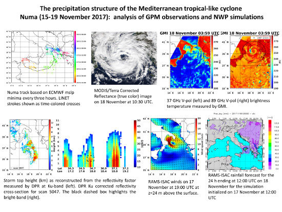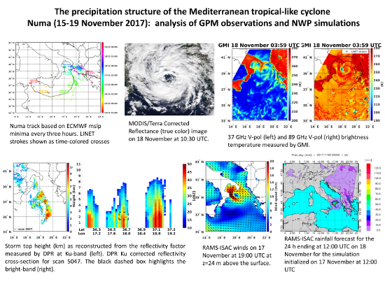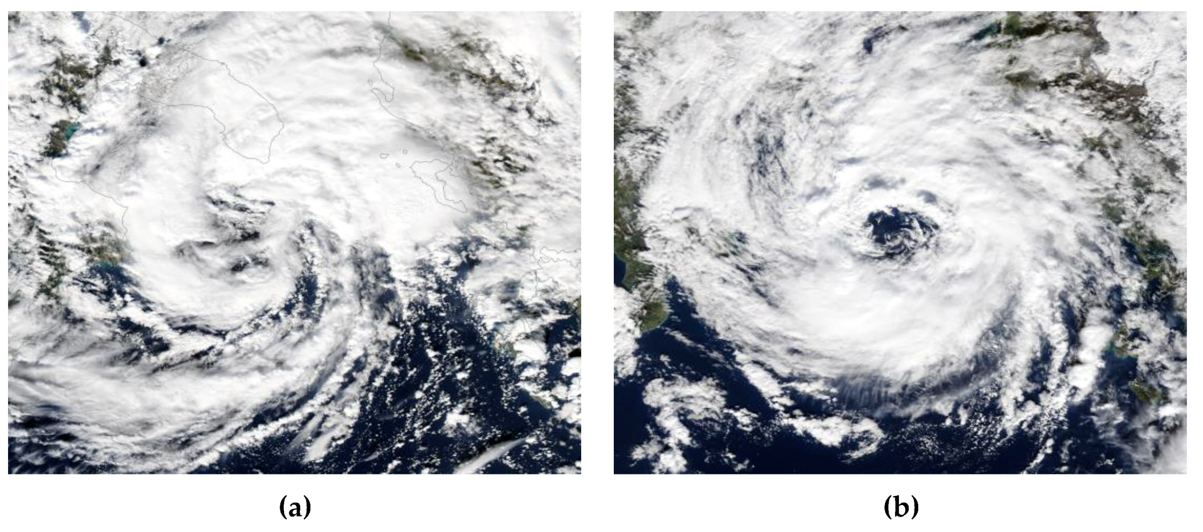Figure 1 shows two MODIS Corrected Reflectance (true color) images capturing Numa as it hits Apulia region and evidences how its upper-level cloud structure changes as subtropical and tropical-like cyclone characteristics alternate. On 17 November at 12:00 UTC MODIS Aqua (Figure 1a) shows a spiral-like cloud band elongated from the center (39.1°N, 18.1°E), with the main rainband in the north hitting the coast of Apulia region, without evidencing an axisymmetric structure or a well identifiable cloud-free eye. On 18 November 2017 at 10:30 UTC, while the storm persists over Southern Apulia region, MODIS Terra (Figure 1b) reveals a well-defined center (39.4°N, 18.7°E) with a cloud-free eye structure, surrounded by a whirl of clouds that appear deeper in the northeastern sector. At both times the storm is characterized by a closed surface wind circulation and a warm core.

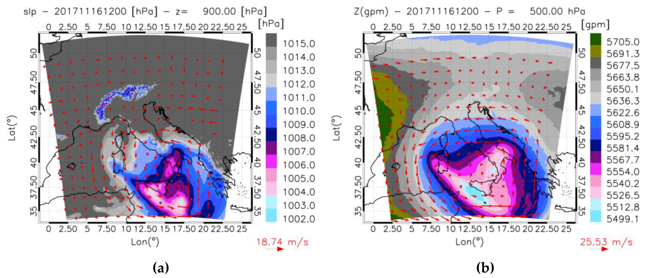
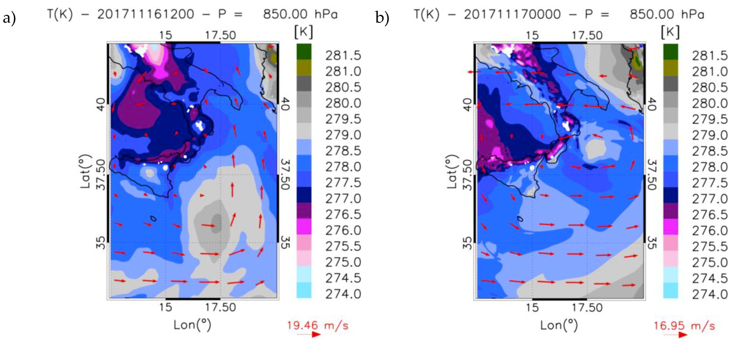
The synoptic environment of Numa both at the surface and 500 hPa is shown by ECMWF operational analyses (Figure 2). On 16 November at 12:00 UTC (Figure 2a,b), a wide low pressure area (minimum 1004 hPa) is present over the Strait of Sicily and over the Ionian Sea, with two distinct minima. The mean sea level pressure (mslp) minimum over the Ionian Sea evolves in Numa, while the minimum over the Strait of Sicily is filled in the following hours. The wind at 900 hPa (red arrows) shows a cyclonic circulation over the Strait of Sicily and Ionian Sea, which is not completely closed around the Numa mslp minimum (Figure 2a). At 500 hPa, the synoptic situation shows a low of geopotential height over Southern Italy with two separate cut-offs. One of them is over the two mslp minima at the surface. Interestingly, the cyclone over the Ionian Sea, evolving in Numa, does not show a warm core surrounded by a close circulation at this stage of development (Figure 3a).

The well-defined mslp minimum, a warm core, as well as the closed cyclonic circulation at 850 hPa, start becoming evident between 16 November 18:00 UTC and 17 November 00:00 UTC (Figure 3b).

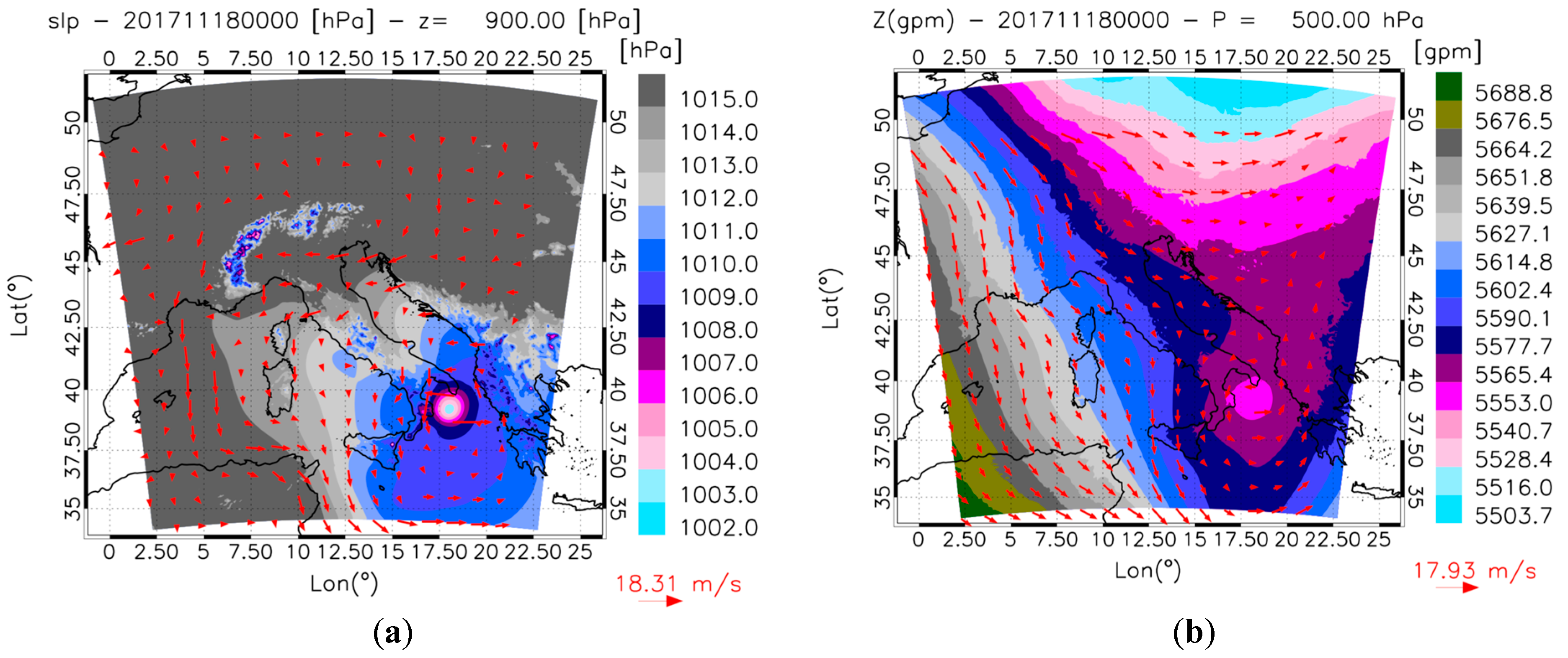
The mslp on 18 November at 00:00 UTC is shown in Figure 4a. The cyclone center is located over the Sea, just offshore the southernmost tip of Apulia region. At 500 hPa (Figure 4b), the geopotential height shows a cut-off and a well-defined cyclonic circulation around its center, which is over the mslp minimum. At this stage of development, Numa clearly shows a warm core at several vertical levels (up to 300 hPa). In particular, at 700 hPa (not shown), the temperature gradient around the Numa center is ~4 °C/120 km.

During the following 12–18 h, the mslp and 500 hPa geopotential height minima were almost stationary in both position and value, causing rainfall and intense winds over Southern Apulia. Thereafter, the storm moved towards Greece while the mslp started to increase.

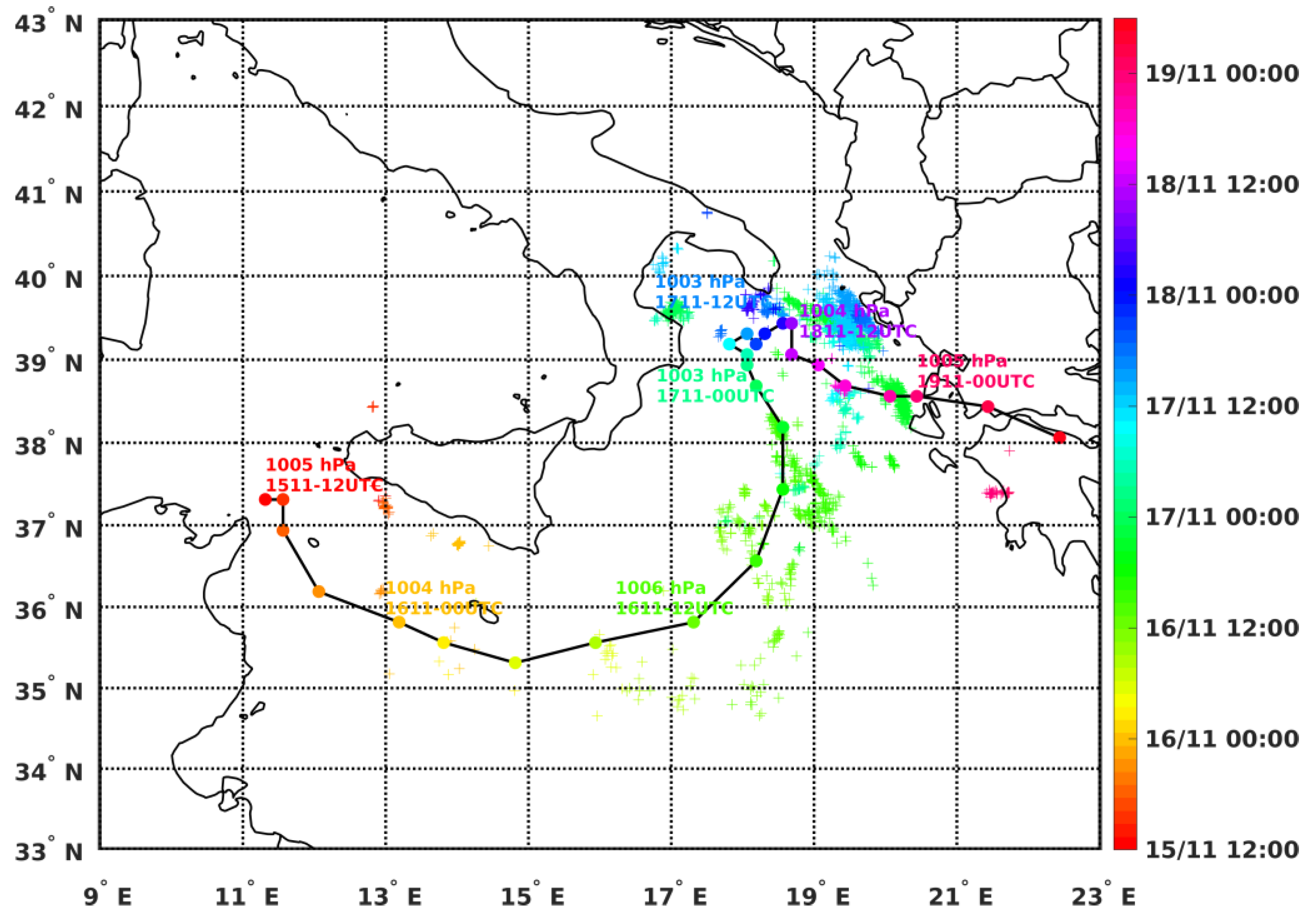
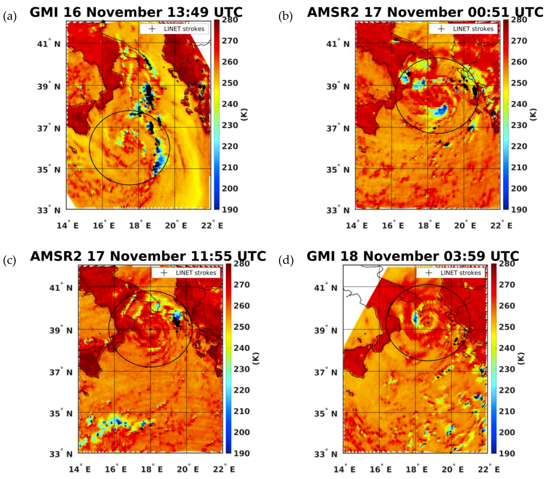
Figure 5 shows the Numa track constructed from the mslp field provided by ECMWF operational analysis/forecast at 0.125°. It illustrates the storm movement traced using the position of the mslp minima every three hours throughout 15 November to 19 November. During its evolution, Numa shows mslp minimum values ranging from 1006 hPa to 1003 hPa, higher than other Medicanes. Figure 5 shows also the lightning activity associated with the storm, as monitored by the LINET network. The total (both CG and IC) strokes detected within 200 km radial distance and within 1 h around the 3-hourly mslp minimum are shown. The persistence of the storm over Southern Apulia region is highlighted by the fact that the same position of mslp minima is found three times for two consecutive 3-hour time intervals between 17 November at 12:00 UTC and 18 November at 12:00 UTC.

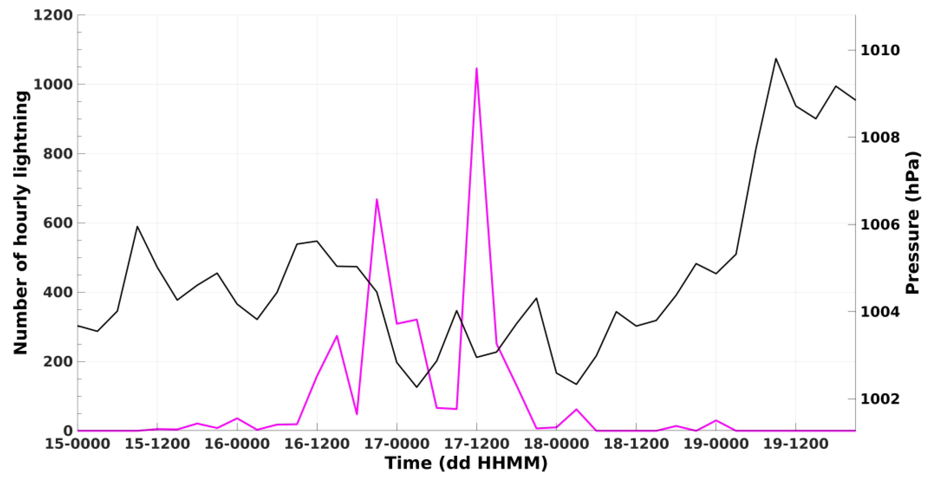
The temporal evolution of the storm in terms of lightning activity and mslp can be seen more in detail in Figure 6, showing the temporal evolution of mslp and the corresponding number of total strokes detected within 200 km radial distance and within 1 h around the location and time of the mslp minima. The figure evidences a more intense lightning activity at the initial stage of the storm when strokes are distributed around the cyclone center. This activity reaches its peak on 17 November at 12:00 UTC after the transition of the storm to the TLC phase. It is worth noting, however, as shown in the next section, that the peak is due to strokes registered in the outer regions of the cyclone, while the lightning activity is absent in the main rainbands in proximity of the cyclone center. As Numa persists over Southern Apulia regions, maintaining its TLC structure, and with the minimum mslp persisting for 24 h over the same area, the lightning activity strongly decreases (Figure 6) because it is confined to the outer regions of the cyclone (at distances > 200 km from the cyclone center). It is worthwhile to note that the LINET detection efficiency is high over the whole domain crossed by the storm throughout its evolution and thus the analysis of lightning activity carried out in this study is reliable.

5. Numa Observations by GPM

Several overpasses of GPM constellation radiometers are available for Numa. Specifically, 53 overpasses are available between 15 November at 12:00 UTC and 19 November at 12:00 UTC, as the storm evolves and moves over the Mediterranean Sea. Fifteen of them capture the storm between 17 November at 12:00 UTC and 18 November at 12:00 UTC, while rainfall persists over the coast of Apulia. It is worthwhile to note that most of these observations occurred during the offshore development of the storm, when ground-based observations were not available.

5.1. AMSR2 and GMI Brightness Temperature Analysis

In Figure 7 and Figure 8, the maps of 37 GHz and 89 GHz TBs for four overpasses by AMSR2 and GMI radiometers over Numa are shown. These two radiometers provide measurements at the highest spatial resolution available in the GPM constellation (~5 km at frequencies > 85 GHz) and are able to depict the precipitation structure with much more detail compared to other MW radiometers [26]. Moreover, the sequence of GMI and AMSR2 measurements and the comparable spatial resolution at each frequency between the two radiometers allow analyzing the evolution of the precipitation at different stages of the storm development.

The 37 GHz channel is particularly suitable for the detection of precipitation because TBs are affected by the combined effect of the emission from the rain layers and the scattering from solid-phase hydrometeors, usually associated with intense updraft (e.g., Panegrossi et al. [49]). Over the sea, in most cases (except in presence of deep convection), precipitation areas appear as regions of high TBs compared to the radiatively cold background surface because the emission by the rain layers dominates the scattering effect at this frequency. Over the land, the emission signal by the surface tends to mask the emission signal by the rain layers. Therefore only heavy precipitation is visible as areas of larger or smaller TB depression. Such depression, which depends on the effect of the scattering on the upwelling radiation, is mostly due to large and dense ice particles found in the convective cores.

In Figure 7, it is evident how the 37 GHz channel, at spatial resolution around 7×12 km² and 8.6×14 km² for AMSR2 and GMI respectively, depicts quite well the location and structure of the rain bands, visible as areas of warmer TBs with respect to the background. The variability of the TB values across the different rainbands originates from the combined contribution of the liquid and frozen hydrometeors within the cloud. Comparing the different panels, it is possible to see that the precipitation structure has changed throughout the storm evolution. The first GPM-CO overpass on 16 November at 13:49 UTC occurs when the storm is at its development stage, more than 200 km off the coast of Sicily and Calabria regions (Figure 7a). At the initial phase the cyclone center is hardly visible, surrounded by a whirling rainband with higher TBs at 37 GHz (up to 260 K) in north/northeastern sector and lower TBs (around 230 K) in the southern sector. The outer rainband extends from the north to the south, on the east side of the cyclone center, while other areas of scattered precipitation extend to the north reaching Southern Italian coastal areas. A wide well-defined eye is visible in both AMSR2 overpasses, on 17 November at 00:51 UTC and at 11:55 UTC, and it becomes narrower and well defined in the GMI overpass on 18 November at 03:59 UTC (Figure 7b–d). The difference of the AMSR2 image at 11:55 UTC (Figure 7c) with respect to the MODIS image shown in Figure 1a is worth noting. AMSR2 shows that the rainfall structure is organized and axisymmetric around the cyclone center, as opposed to the upper level clouds which do not show evidence of a well-defined cloud-free eye. On 17 November, the AMSR2 maps at 37 GHz show that the cyclone center moves from 38.5°N 18.5°E to 39°N 18°E (~70 km) in 12 h, while areas of higher TBs with values around 260 K are found mostly in the northern sector of the storm, over the Ionian Sea. Specifically, at 00:51 UTC an area of high TBs is found in correspondence of the outer rainfall structures in the northern sector of the cyclone, extending to the Calabria region (visible as an area of slight TB depression over land compared to the background), while at 11:55 UTC, this area is part of the main rainband around the cyclone center, hitting the coast of Salento in Southern Apulia region.

The absence of areas of significant TB depression at 37 GHz might be due to one or a combination of the two following factors: (1) the absence of high amounts of large high density ice particles, that significantly scatter the upwelling radiation at 37 GHz; (2) the low spatial resolution of the 37 GHz channels, that cannot distinguish small convective cores. An ambiguity at this frequency comes between the regions of precipitation with no significant contribution of the ice to the scattering (optically thin clouds), and the regions of strong precipitation and significant ice scattering (optically thick clouds). The ambiguity is solved looking at the other channels. For example, maps of TBs at 10 and 19 GHz (not shown), mostly affected by the emission from the rain layers, can be more directly related to rainfall intensity (especially at 10 GHz in Rayleigh regime) with higher values of TBs generally associated with heavier rainfall. However, since they are available at lower spatial resolution (24 × 42 km² and 14 × 22 km² for AMSR2, at 10 GHz and 19 GHz respectively), they do not allow to depict clearly the rainband structure.

The TBs measured by GMI and AMSR2 at 89 GHz (V polarization) are shown in Figure 8, along with the LINET strokes registered within 1 h around the time of the overpass. At this frequency water vapor emission increases the TB background values. In correspondence of the clouds, the upwelling radiation is affected by the emission of cloud liquid water, which tends to further increase the TBs, and by the scattering by the ice hydrometeors (mostly those found in the convective regions) visible as areas of higher or lower TB depression (e.g., [50]). In the development stage, captured by the GMI overpass on 16 November (Figure 8a), most of the clouds in the outer rainbands show significant TB depression compared to the background. The TBs as low as 158 K in the southern portion of the rainband (35.23°N, 19.07°E) suggest the presence of strong convective activity [51,52,53], associated with significant amounts of ice, presumably either heavily rimed ice or high density graupel. On the other hand, in the two AMSR2 images on 17 November (Figure 8b,c), the area surrounding the cyclone center, exhibiting a symmetric rainfall structure at 37 GHz, does not show any scattering signal (a ring of higher TBs in correspondence of the eyewall is evident in Figure 6c), indicating that rainfall mostly originates from warm rain processes. Scattering signal is evident in some regions of the outer rainbands in the AMSR2 overpasses, including the significant TB depression area over the Ionian Sea and over Calabria region at 00:51 UTC, and over the coast of Salento region at 11:55 UTC. The areas of TB depression are closer to the cyclone center as the storm persists in its mature stage (GMI overpass on 18 November – Figure 8d), while the eye becomes smaller and well defined (MODIS image in Figure 1b), clear indications of the intensification of the storm. In this phase, only a small portion of the rainbands on the west side of the cyclone eye shows significant TB depression at 89 GHz. The lack of very low TBs at 89 GHz (minimum 191 K at 39.38°N 17.93°E) compared to typical convective systems (as categorized in [51,52,53]), and the absence of scattering signal at 37 GHz, are a clear indication of a weak convective activity associated with Numa during its TLC stage. Coherently with what observed in Figure 5, Figure 6 and Figure 8, the electrical activity is more intense during the development stage of the Medicane. More specifically, 177 strokes (IC 10 - CG 167) in one hour are detected by LINET for the first overpass, while only 8 strokes (IC 2 - CG 6) occur during the mature stage, within 200 km from the position of the eye. Overall, the number of strokes registered is low compared to typical convective systems observed in the Mediterranean (see also [26] and [27]). Figure 8 shows that the electrical activity is mostly located in correspondence with the areas of lower 89 GHz TBs during the development phase, while it is absent in the cyclone center and in correspondence of the TB minima at 89 GHz during the TLC phase. During this phase, the lightning activity is mostly found in correspondence with the convective clouds at the edge of the cyclone. It is clear that the peak shown in Figure 6, found on 17 November at 15:00 UTC, is associated exclusively with the convection in the outer regions of the storm.

The spatial distribution of the regions of lower TBs at 89 GHz changes throughout the storm evolution, while the rainfall pattern shown at 37 GHz maintains a symmetric structure around the eye (with variable intensity). GMI channels above 89 GHz (not shown), sensitive to the scattering of frozen hydrometeors found in the upper cloud layers in the regions of the outflow, show slight TB depression, mostly in correspondence with 89 GHz rainband pattern, and more evident during the development phase. The lack of scattering signal at higher frequency (> 150 GHz) in correspondence of the cloudy areas of the MODIS VIS image shown in Figure 1, associated with the strong depolarization signal at 89 GHz (not shown), is an indication that the upper cloud layers in the Medicane during its TLC phase may be characterized by the presence of supercooled cloud droplets.

5.2. GPM-CO Precipitation Product Analysis

Panegrossi et al. [28] have carried out a comparison of the precipitation retrieved from the AMSR2 and GMI overpasses shown in the previous section. Here we focus on the precipitation products available from the GPM-CO overpasses.

For the GPM overpass over Numa on 16 November at 13:49 UTC, both GMI and DPR observations are available. The availability of the radar observation allows for a 3D insight of the storm. The reflectivity factor measured by the DPR is a proxy of the storm top height (Figure 9a). It is worth noting that the storm top height could be underestimated, because of the low sensitivity of the DPR (both Ku and Ka band) unable to detect the small ice particles in the upper cloud layers.

At this stage of the storm development, the 3D structure provided by the DPR shows the presence of a quasi-cloud free region around the storm center (as identified by the mslp minimum at the time of the overpass) surrounded by clouds (precipitation) reaching a maximum height of about 6 km. Along the northwest to southeast direction, on the eastern side of the storm center, there is a rainband as high as ~10 km. The limited Ku-band swath width does not allow analysis of the system on the western edge of the storm, but the GMI measurements (Figure 7 and Figure 8) evidence that there are no rainbands developing in that region.

Thanks to the availability of co-located radar and radiometer observations, the DPR Ku measurements can be related to the GMI TB behavior and to the 3D structure of the storm. To this end, we consider the vertical cross-section of the Ku-band reflectivity, corrected from attenuation effects (Z_c), along the across-track DPR Ku/Ka scan 5047 (indicated by the black dashed line in Figure 9a), and shown in Figure 9b.

It is evident the coexistence of convective cores (e.g., 37.1°N, 18.8°E) embedded in stratiform regions (e.g., 36.7°N, 18.0°E) in the rainband. The shallow convection activity can be easily inferred from the high value of Z_c, that is about 50 dBZ up to 4 km. These convective cores seem coincident with the areas of lower TBs at 89 GHz and intense lightning activity, shown in Figure 8a. On the other hand, the presence of stratiform clouds is evidenced by a signature of bright-band (BB) in some portions of the rainbands, i.e., a peak of Ku-band reflectivity factor in the vertical profile due to melting ice particles, more evident in other along-track cross-sections (as shown in Panegrossi et al. [28]). The height of the BB signal is coherent with the freezing level height (~2400 m) inferred from the corresponding ECMWF reanalysis temperature profile.

The precipitation rate estimated by GMI, obtained from the combination of the information provided by all the channels available, is shown in Figure 10a. It can be compared with the precipitation rate estimated from the Ku-band DPR measurements, shown in Figure 10b (the precipitation rate estimate from Ka-band is not shown because of its narrower swath, compared to DPR Ku-band). In the region of the storm seen by both instruments, there is a relatively good agreement between the patterns of precipitation, especially considering the nonuniform beam-filling effect related to the lower spatial resolution of the radiometer (in particular for the low frequency channels < 37GHz) compared to the DPR, the different viewing angle, and the different approaches used for DPR and GMI to retrieve the surface precipitation. DPR shows very small areas of high rainfall rate which appear smoothed out in the GMI retrieval. As a matter of fact, the highest precipitation rate estimated from GMI is found in the southern portion of the main rainband around 35°N, where TBs at 89 GHz show an extended area of minimum values in Figure 8, and it is 19 mm/h, while the maximum DPR estimate is ~80 mm/h in that region.

Comparing the GMI precipitation rate map in Figure 10 with the TBs at 37 GHz (Figure 7a,d), it is evident that lower TBs, found in the development phase compared to the mature phase, are due to the scattering by the ice hydrometeors in the convective cores (shown by DPR cross-section), which tends to mask the emission signal by the rain layers.

For the GMI overpass on 18 November at 03:59 UTC, when Numa hits the coast of Southern Apulia region, the pattern of the precipitation (Figure 11a) follows the pattern of the TBs at 37 GHz (over the sea), with peaks around 14 mm/h in the region of minimum TBs at 89 GHz in the main rainband. DPR observations are not available for this overpass, because the storm is outside the Ku-band swath. However, a portion of the storm at this time lies within the field of view of the C-band Doppler dual polarization ground radar (GR) located in Pettinascura, Calabria region, managed by the Department of Civil Protection of Italy. Unfortunately, for this event only single polarization and Doppler radar volumes at 1 km radial resolution were available.

The GPROF GMI rainfall rate, shown in Figure 11a, is compared with the rainfall rate estimated from the GR observations available at the time of the GMI overpass (Figure 11b). At this time the cyclone eye is 150 km from the radar site, and the radar shows portions of two rainbands, one of them closer to the radar site, which are fully observed by the GMI.

From the visual comparison of GPROF GMI and GR rain rate products shown in Figure 11, we note that the GMI rainfall rate estimate for the western rainband is in very good agreement with the GR rainfall rate estimate, showing values as high as 5 mm/h. However, we note a disagreement in terms of rainfall rate intensity for the eastern rainband (approximately centered at 39.5°N, 18°E), which appears to be more intense in the GPROF GMI products than that shown in the GR map. This discrepancy in the retrieved rain rate intensity could be explained by considering the slanted GR viewing geometry that constrains the GR near-surface bin height (NSBH) to progressively increase with the distance from the radar site. Thus, at longer distance the near-surface rain rate estimation is expected to be of lower quality. Figure 12 shows the GR perspective of the western and eastern rainbands positioned at ~50 km and ~120 km from the radar, with reflectivity factor peaks of the order of 30 dBZ and 20 dBZ, respectively. To compare more in detail GPROF GMI vs. GR, in Figure 12 the GMI TBs are superimposed to GR reflectivity. This comparison confirms that the eastern rainband, with larger TB depression at 166 GHz and 89 GHz (150K and 210 K, respectively), corresponds to the radar raincell having larger vertical extension, but higher NSBH and lower GR rain rate. On the other hand, the western rainband, with smaller 166 GHz and 89 GHz TB depression (210K and 240K, respectively) shows a radar raincell with a smaller vertical extension but with lower NSBH and higher GR rain rate. Path attenuation produced by the western radar raincell could be an additional element to explain the radar rain rate underestimation of the eastern raincell. This is supported by the consistency between the freezing level height (which is expected to be at 2400 m as previously reported) and the core of the western raincell (which extends from 1700 m to 2500 m). In this situation, the core of the western raincell may likely partially attenuate the lower end of the eastern cell thus compromising its near-surface precipitation retrieval.

6. Analysis of RAMS-ISAC Simulations

The forecast of Medicane Numa was characterized by a significant change of the prediction of its position depending on the model initialization time. In an unstable flow regime, such as Numa, the sensitivity of the predicted storm features, for example the position of the cyclone eye, to the initial and boundary conditions is well known [5,13]. Nevertheless, in this section we highlight important aspects related to an operational NWP model setup [13]. Here we analyze the operational RAMS-ISAC forecasts issued on 16 and on 17 November. The first operational forecast uses the Global Forecast System (GFS) analysis/forecast cycle issued at 12:00 UTC on 16 November as initial and boundary conditions, while the second forecast uses the GFS analysis/forecast cycle issued 24 h later at 12:00 UTC on 17 November. GFS initial and dynamic boundary conditions are downloaded at 0.25° horizontal resolution. The boundary conditions are updated every 6 h and the finalization date is +60 h after the initialization time. The sea surface temperature (SST) is interpolated onto the RAMS-ISAC grid from GFS analysis at 0.083° horizontal resolution. SST is constant during the simulation and it is that of the initial time of the simulation (12:00 UTC on 16 and 17 November, depending on the simulation).

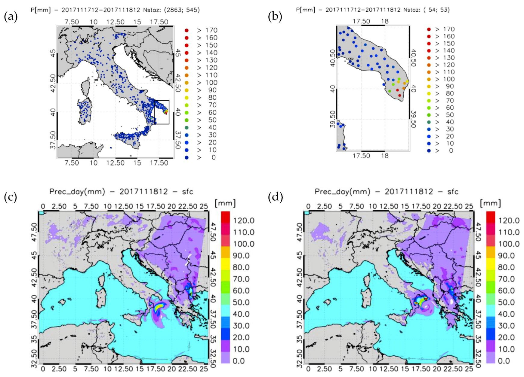
It is important to note that we do not consider the impact of rapidly generated sea waves on the sea surface roughness, which plays an important role for the exchange of energy and momentum between the sea surface and the atmosphere. The sea surface roughness is estimated by the Charnock relation [54], which increases with the square of the friction velocity. So, the sea surface roughness is higher for more intense surface winds. We used rain gauges to independently verify the accuracy of the forecasts. Based on rain gauges, the most abundant precipitation registered over land during the event was in the southern part of the Apulia region (Salento), between 12:00 UTC on 17 November and 12:00 UTC on 18 November. The Italian rain gauge network (Figure 13a,b) recorded 24 h precipitation varying from 64 mm/24h of Corigliano d’Otranto (40.1°N, 18.3°E) to 172 mm/24h of Presicce (39.9°N, 18.3°E), with the second largest precipitation (147 mm/24h) in Ruffano (40.0°N, 18.3°E). It is worth noting that the mean annual (monthly) precipitation in Salento is ~810 mm/year (~125 mm in November) and that the 17–18 November 2017 event was the most intense in terms of 24h cumulated precipitation since 1970 [55].

Figure 13c shows the 24 h precipitation predicted between on 17 November at 12:00 UTC and on 18 November at 12:00 UTC for the simulation starting on 16 November at 12:00 UTC. The amount of 100 mm/24h is predicted over the Ionian Sea, with the maximum found 50 km south of the Apulia coast. Precipitation is predicted also over Calabria (39.7°N, 16.8°E) with maximum amounts of 90 mm/24h. While the forecast shows that Numa could be a potentially dangerous meteorological system because, in addition to the high winds, it brings considerable precipitation, the forecast on 16 November shows small precipitation amounts over Apulia, and northeastern Calabria. The situation is different for the forecast issued on 17 November (Figure 13d); in this forecast, the impact of Numa in Southern Apulia is evident, because RAMS-ISAC shows a maximum of 140 mm/h and 120 mm/24 h in Presicce and Ruffano, respectively, in good agreement with the observations.

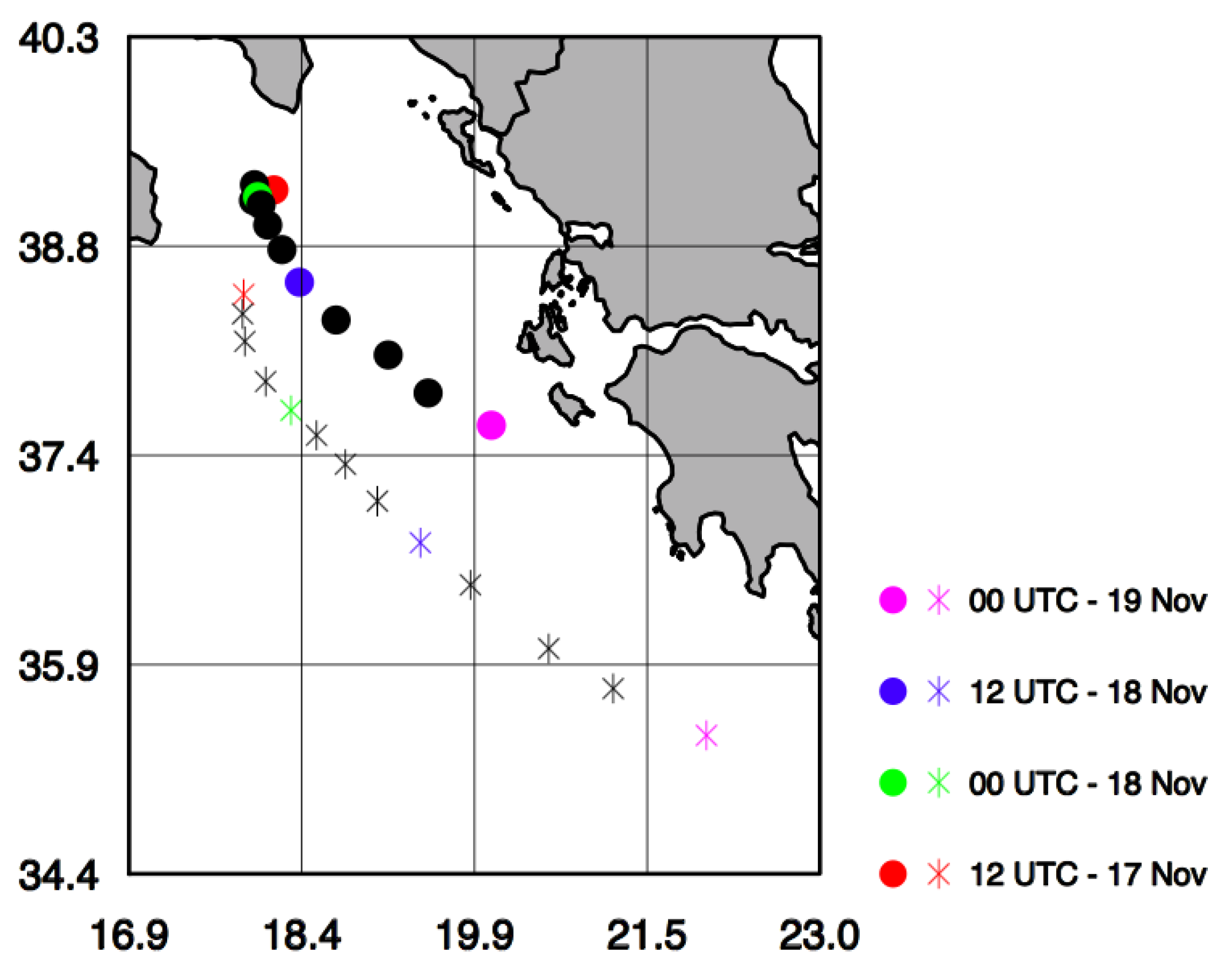
Interestingly, the simulation starting at 12:00 on 16 November was able to forecast the TLC features of Numa, similarly to that on 17 November (see Figures 15 and 16) and, considering the characteristics of the storm (low vertical wind shear, quasi-neutral moist environment, sea level pressure minima, amount of precipitation at the surface, etc.), the two forecasts issued on 16 and 17 November are similar. Nevertheless, an important difference arises comparing the storm tracks of the two simulations (Figure 14). The storm track of the forecast issued on 16 November (R16) is shifted to the south compared with that issued on 17 November (R17). Also, while the R17 storm track is almost stationary for the first 12 h, the R16 center of the storm moves more rapidly towards Greece. The R17 track is in better agreement with that of Figure 5 which, being derived from ECMWF analysis and short-term forecast, can be considered as the reference. The mslp minima have similar values between R16 and R17 and vary from 1003 hPa to 1006 hPa, in good agreement with values in Figure 5.

From the above analysis, it follows that the differences between R16 and R17 are mainly in the tracks followed by the TLCs of the two simulations, showing the important role of initial and boundary conditions for the forecast of this kind of events, similarly to other studies ([5,13] among others). Therefore, the consequences on the precipitation field forecast over the land are significant.

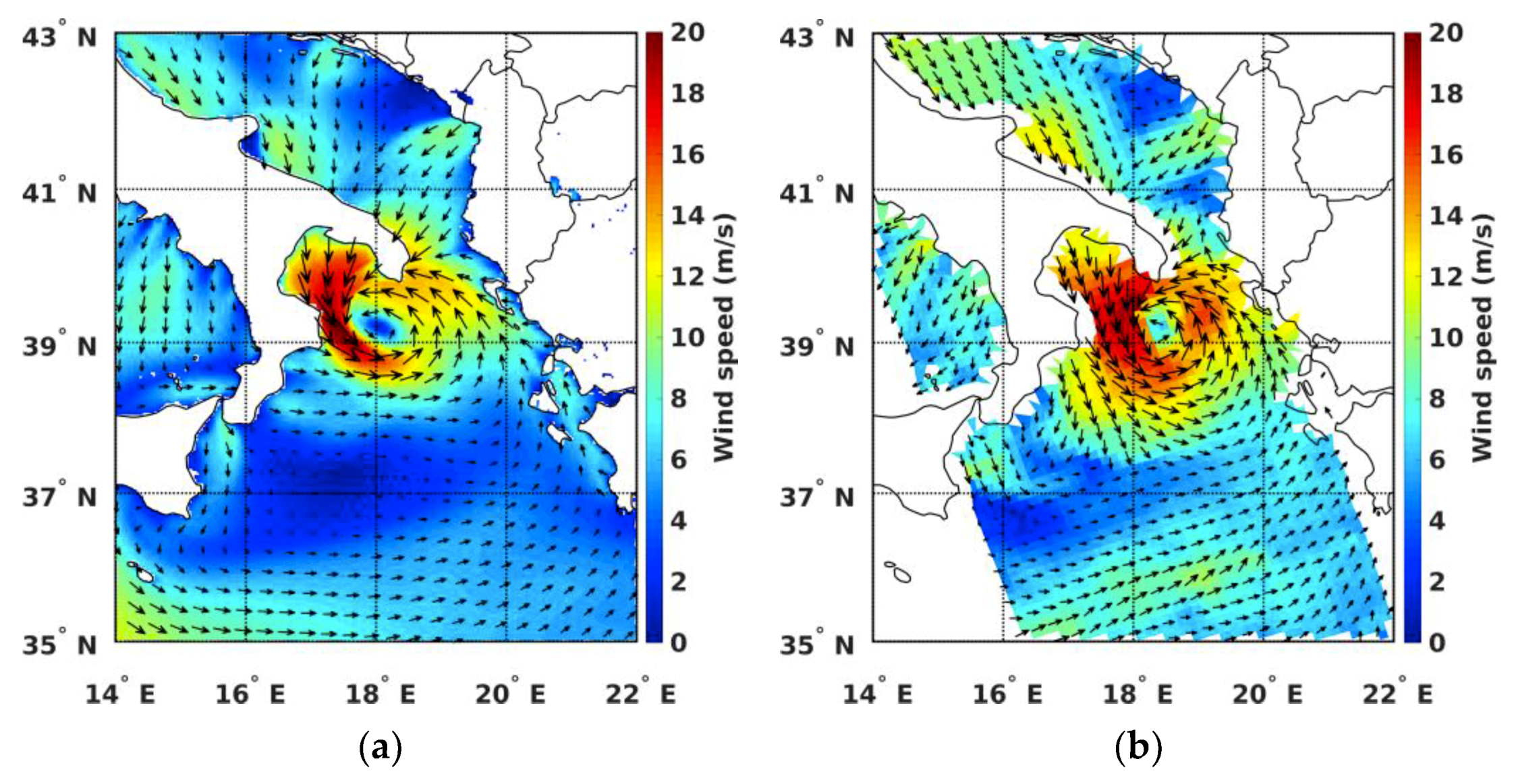
Since the simulation starting on 17 November at 12:00 UTC provides a good rainfall field forecast over Apulia region, in the following the output of this simulation is used to present some characteristics of Numa TLC phase. An important feature of the Medicanes is the surface wind, which can be intense, causing damages and being a threat for the populations. Satellite observations are an important source of data in this context because they can be used to verify the wind field forecast over the sea, where conventional observations are sparse. Figure 15 shows the comparison between RAMS-ISAC forecast on 17 November at 19:00 UTC, and the ASCAT observations at 19:09 UTC on the same day. The model is able to predict several features of the storm, such as the eye position (shifted few kilometers to the southwest of the real position) and the strong wind, up to 20 m/s, on the western side of the eye. The main areas of moderate-intense wind over the Adriatic and Ionian Seas are also well predicted even if the model underestimates observed winds. There are also local scale features that are not forecast by the model, as the local wind patterns south of 37°N and east of 18 °E.

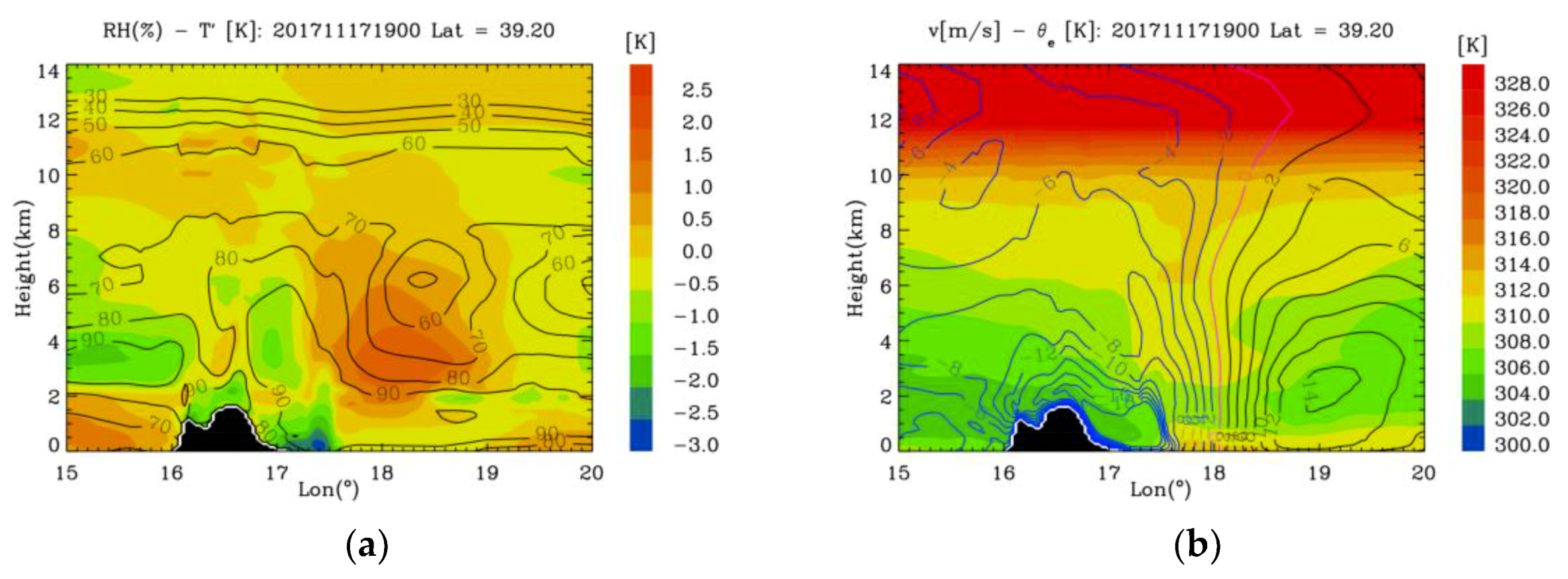
As already stated, Numa shows TLC features at this time of development. To highlight these features, Figure 16a shows the cross-section of relative humidity and temperature anomaly fields along 39.2° N latitude on 17 November at 19:00 UTC. The temperature anomaly is computed with respect to the mean value at each vertical level. The warm core caused by the release of the latent heat of the evolving TLC extends from 1 km to 10 km height (with 1.5 K anomaly between 2 and 5 km height), showing a deep vertical extension of Numa. Relative humidity is lower in the warm core region. It is higher below 2 km height and in the outer regions of the TLC, indicating (a) low-level moisture convergence and (b) moisture redistribution by the convection.

Figure 16b shows the vertical cross-section, at the same latitude of Figure 16a of the equivalent potential temperature and of the meridional wind speed. Typical features of TLC are apparent as the state of nearly-moist neutrality of ascending air parcels, the limited horizontal extension of the TLC, the axisymmetric shape, the windless region in proximity of cyclone center (the TLC calm eye), and the low vertical wind shear up 6 km height [5,7,13].

The results of Figure 16a,b indicate that the so-called Wind Induced Surface Heat Exchange (WHISHE [56,57]) may play an important role in Numa TLC phase maintenance.

7. The Implementation of DPR (Dual Frequency Precipitation Radar) Reflectivity Observation in RAMS-3Dvar

In this section we show the implementation of DPR 3D reflectivity field as an observation in the RAMS-ISAC data assimilation scheme. The RAMS-3DVar assimilation scheme [39] modified to assimilate reflectivity factor observed by ground radars [58] is used for this purpose. The background is given by a short-term forecast of the RAMS-ISAC. More specifically, since the DPR observation is available at 13:49 UTC on 16 November, we use the background at 14:00 UTC neglecting the time difference between the DPR observation and the RAMS-ISAC background. The DPR reflectivity is sampled at seven vertical levels from 2000 m to 8000 m to match the model vertical bins, and is assimilated following Caumont et al. [59]. Hereafter, the simulation with no DPR assimilation is referred to as CTRL, while the simulation with DPR assimilation is referred to as ANL.

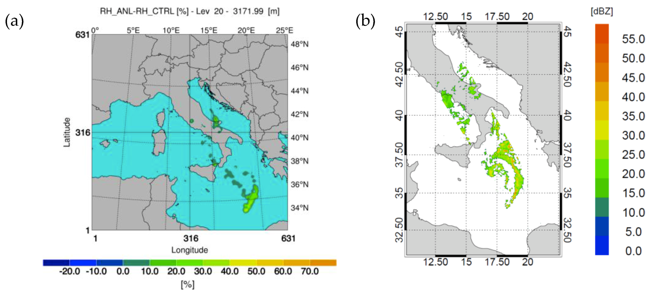
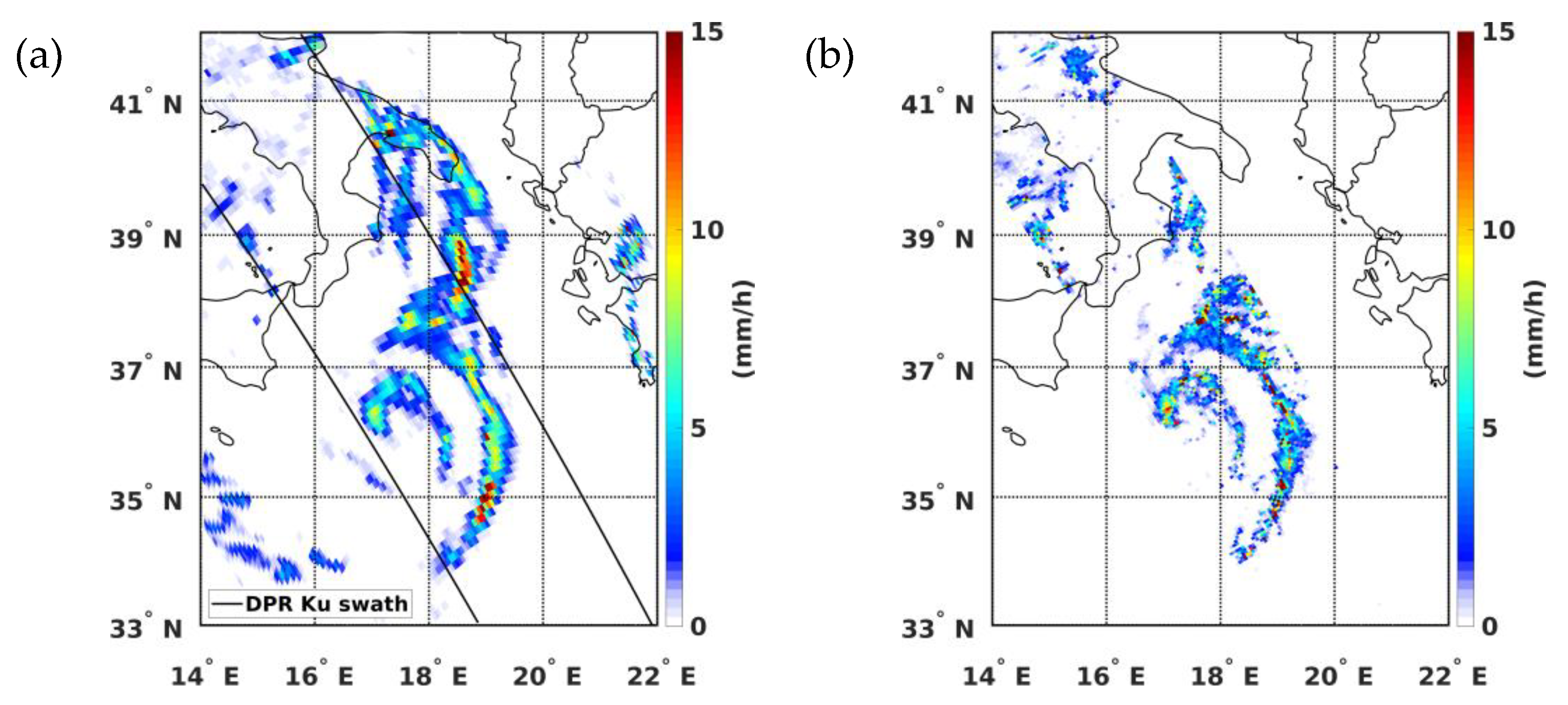
Figure 17a shows the difference between ANL and CTRL forecast of the relative humidity (RH) field at 14:00 UTC, at 3172 m in the terrain following coordinate system used by RAMS-ISAC. There are several areas of the domain where the assimilation increases the relative humidity of the model (RH difference up to 30%). For comparison, Figure 17b shows the DPR reflectivity at 3000 m at 13:49 UTC, quantifying the impact of the DPR reflectivity assimilation on the RH field. The largest impact on the forecast is introduced south of 36°N, in correspondence of the main “comma”-shaped rain band observed by DPR (see Figure 10b). The RH perturbation is significant and, once assimilated into the model, it may determine saturation and precipitation where/when introduced. Other perturbations to the RH field are given in Northeastern Sicily and in Central-Eastern Italy.

As stated above, the DPR data are assimilated at 14:00 UTC on 16 November. As shown in the previous section, the forecast starting on 16 November at 12:00 UTC missed the precipitation over Southern Apulia 24–48 h later (between 17 November at 12:00 UTC and 18 November at 12:00 UTC). The DPR reflectivity assimilation is not able to correct the precipitation forecast in Southern Apulia, likely because the (only) DPR overpass is available 24 h before rainfall hits Southern Apulia. This result is similar to other studies with radar data assimilation (see Hu et al. [60] and Jones et al. [61]), showing that the resilience of the impact of the assimilation is about 6 h.

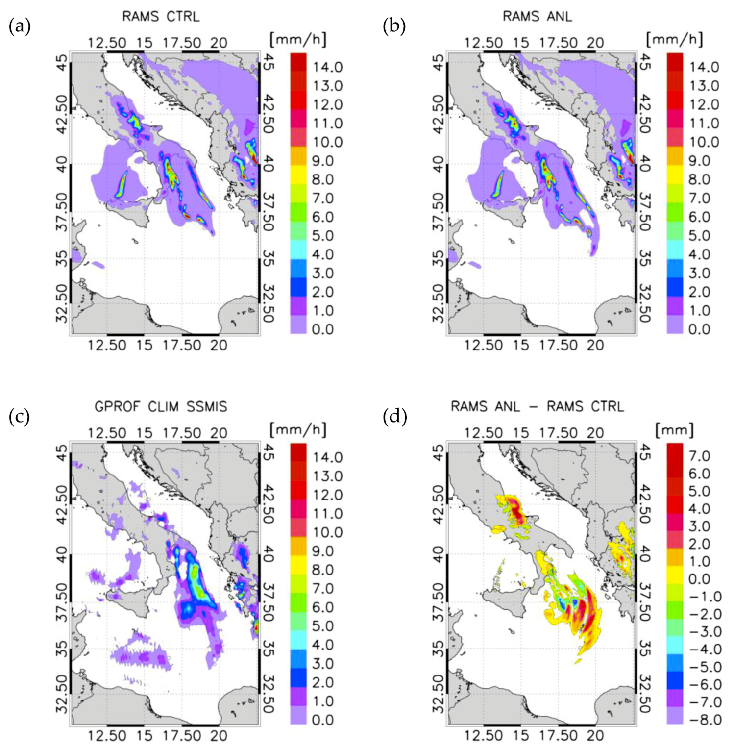
Nevertheless, weak effects of assimilating DPR can be seen in the comparison of the CTRL and ANL precipitation rate at 16:20 UTC (Figure 18), i.e., 2h and 20 minutes after the assimilation time, when an SSMIS overpass is available and captures the storm during its transition over the Ionian Sea. The precipitation rate field is compared to that obtained from the NASA GPROF-CLIM-SSMIS V05 product. The comparison shows important differences between SSMIS precipitation rates and both ANL and CTRL. This difference is caused by both forecast errors, and the low spatial resolution of the GPROF precipitation rate (SSMIS has spatial resolution three times lower than GMI and AMSR2). Nevertheless, the GPROF-CLIM-SSMIS rainfall pattern shows precipitation south of 36°N and west of 18°E, which is not simulated by CTRL forecast.

ANL precipitation, however, extends more to the south compared to CTRL and, in particular, it extends to 35°N latitude and east of 18°E, in better agreement with GPROF-CLIM-SSMIS precipitation pattern. The southward shift of the ANL precipitation is confirmed by the comparison of the CRTL and ANL accumulated precipitation between 14:00 UTC and 18:00 UTC (Figure 18d). In this case differences up to 7 mm/4h are predicted south of 37°N. The southward extension of the precipitation forecast of ANL compared to CTRL is a consequence of DPR data assimilation, as shown in Figure 17a.

As shown above, the assimilation of the DPR reflectivity did not have a significant impact on the simulation of TLC Numa. However, the above results show the possibility to implement DPR reflectivity as an observation in data assimilation systems, leaving the question of its impact on the forecast open.

8. Discussion

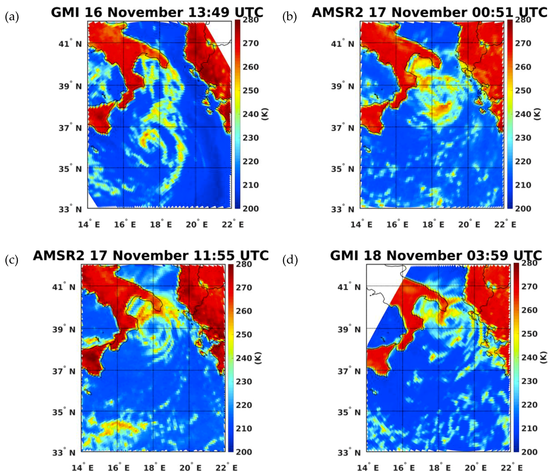
The analysis carried out for Medicane Numa highlights how powerful MW radiometers are in identifying the details of its precipitation structure, not discernible in conventional (VIS or IR) satellite imagery, as it evolves over the Mediterranean Sea. This is particularly evident for AMSR2 and GMI, thanks to their high spatial resolution compared to the other radiometers. The behavior of the measured TBs (at 37 and 89 GHz for example) is a clear indication that the main precipitation formation mechanism in the storm during its TLC stage, and in particular in the rainbands around the eye, is likely slantwise convection characterized by a weak updraft. Ice hydrometeors show different scattering properties from those found in the high convective cores (high TB minimum at 89 GHz, absence of scattering at 37 GHz, and no electrical activity). As the eye becomes more defined and the cyclone strengthens, the main rainband shows signatures of weak convection at 89 GHz (and at higher frequencies), due to scattering by precipitation-size frozen hydrometeors. However, even in this case, the absence of strong vertical motions inhibits the electrical activity. The analysis of GMI TBs and surface rainfall rate at the development phase evidences stronger convection activity. The minimum Polarization Corrected Temperature (PCT) at 89 GHz, computed according to [62], is 160.65 K and 195.35 K, in the development phase and in the mature phase of Numa, respectively. The 30 K difference of the 89 GHz PCT minimum values confirms that the convective activity is much weaker in the mature phase than in the development phase, in agreement with what found in previous studies (e.g. [3]). Comparing these values with TMI climatology of convective systems (e.g., Cecil et al. [51] and Liu and Zipser [52]), it is evident that the convection identified during the mature phase can be characterized as “weak”, whereas during its development phase Numa shows features typical of “strong” convection. The lack of scattering signal at higher frequency (> 150 GHz) in correspondence of the MODIS VIS cloud image during the TLC phase, and the depolarization at 89 GHz, indicate the presence of supercooled cloud droplets. The GMI and AMSR2 TB behavior finds correspondence to what found in other studies about in situ observations in tropical cyclones [63,64,65]. They confirm that tropical oceanic convection is usually not known for the strength of its updraft (exceptions occasionally occur), which is required to loft substantial quantities of rain drops and dense graupel to high altitude. In situ observations evidence, instead, the presence of supercooled cloud droplets at high levels and that the ice, mostly rimed particles and low density graupel, forms in the weak updraft regions and is redistributed throughout the storm by the upper and midlevel outflows.

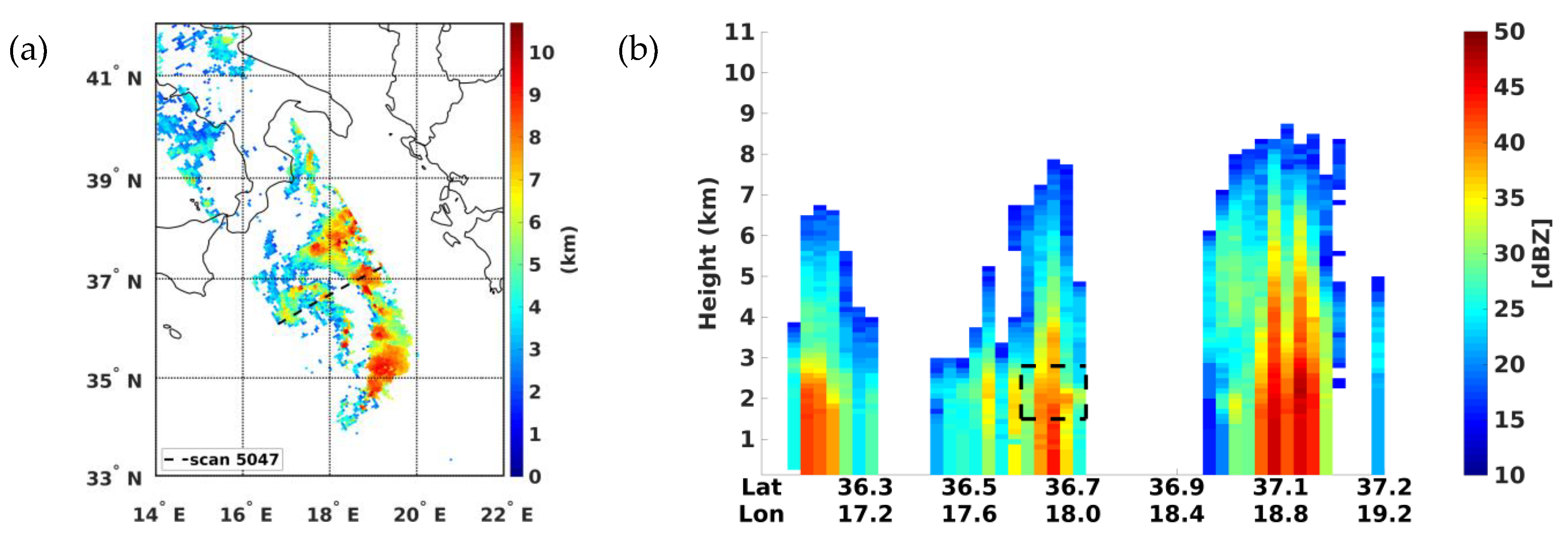
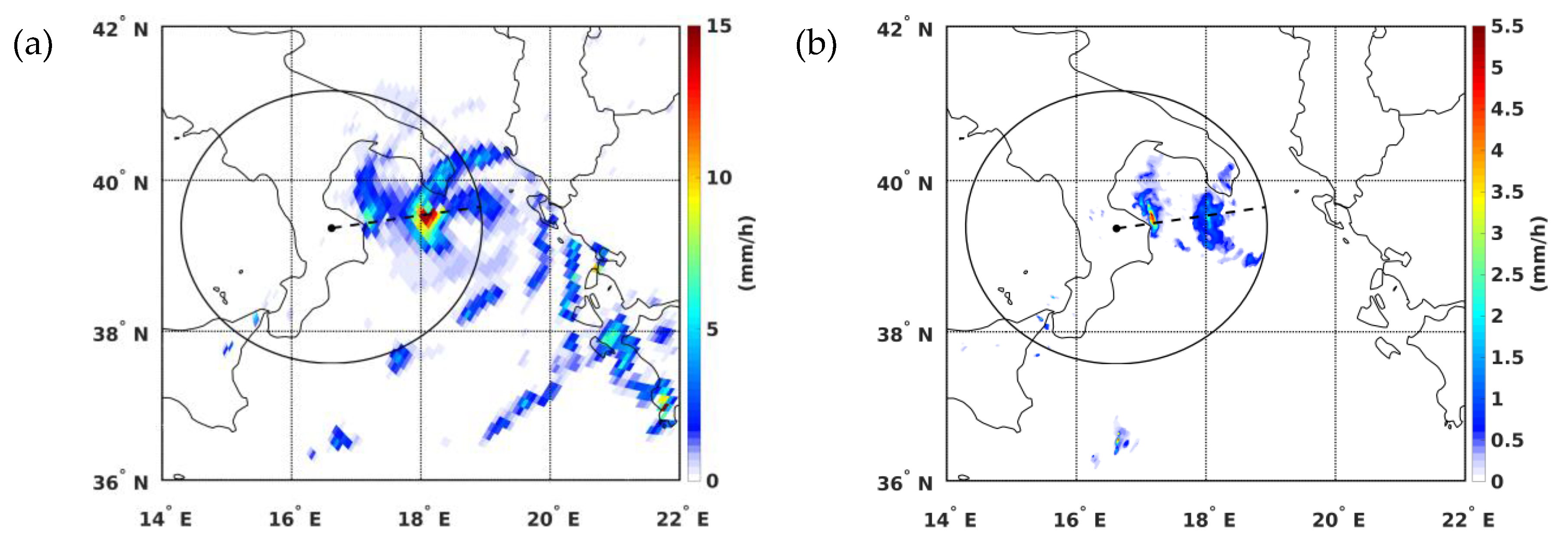
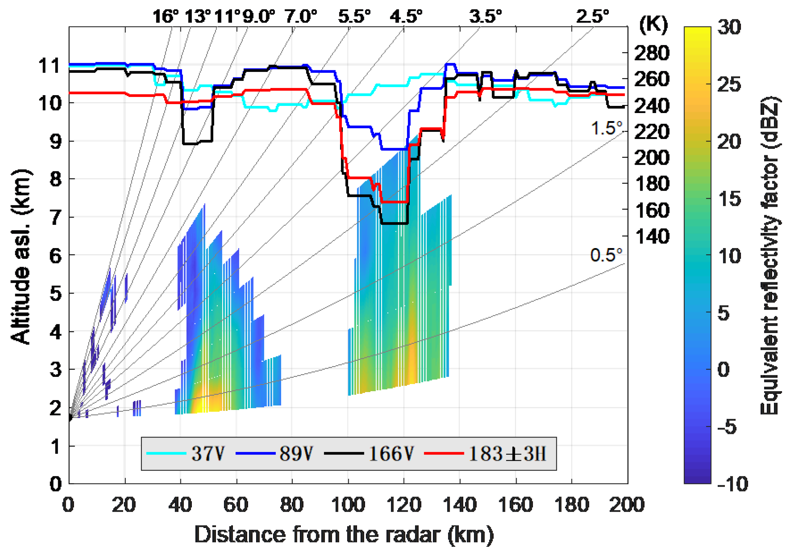
In the development phase, we have analyzed for the first time the 3D structure of this kind of storms, as observed by a spaceborne radar. DPR is particularly valuable because it can provide information on the storm features, from both the microphysical and meteorological perspective, thus supporting what already evidenced by the GMI TB analysis. On the other hand, during the TLC phase, GMI allows highlighting precipitation underestimation by the ground radar of Pettinascura, mainly due to the blind zone caused by its viewing geometry. In fact, the area of Numa, although frequently hit by Medicanes or intense precipitation, is not yet adequately covered by operational weather radars. These results confirm that spaceborne MW observations can provide useful insights about rainfall structure, intensity, and pattern, especially over the sea where no ground-based data are available, and when GR rainfall rate estimates might be affected by large uncertainties (as shown also in Panegrossi et al. [26]).

The investigation of numerical modeling performance has shown that the RAMS-ISAC forecast for this event is sensitive to the initial and boundary conditions. In particular the forecast starting on 16 November at 12:00 UTC was unable to correctly predict the landfall over Apulia, while the forecast starting on 17 November at 12:00 UTC correctly predicted the rainfall amount and landfall over Apulia. The storm track simulated on 16 November is too far south from the real path, and rainfall was forecast mainly over the sea. The simulation starting on 17 November shows a good prediction of the precipitation field and was used to gain insight into the TLC phase of Numa. Wind speeds up to 20 m/s were simulated on 17 November at 19:00 UTC, in good agreement with ASCAT observations. The warm core extended up to 10 km showing a deep vertical extension of Numa, favored by the long-lasting TLC phase [18]. Other TLC characteristics as the small horizontal extension of Numa, the low vertical wind shear, the axisymmetric shape, and the calm eye of the Medicane, were well captured by the model. These results, in agreement with previous model-based studies on Medicanes (e.g. Lagouvardos et al. [2], Miglietta and Rotunno [5], Davolio et al. [13], Picornell et al. [21]), support the passive MW observation analysis, showing that during the TLC phase warm rain processes occur in the area surrounding the eye, while weak convective activity is observed in small portions of the eyewall. We have analyzed how DPR measurements, available over the sea, can be also used in NWP data assimilation. However, because only one overpass of the DPR is available, the impact of the data assimilation on the Numa forecast was limited. Nevertheless, DPR reflectivity data assimilation caused an extension of the rainfall forecast toward the South, in better agreement with NASA GPROF-CLIM-SSMIS V05 product.

9. Conclusions

In this study a Medicane event, named Numa, which occurred in November 2017, has been investigated by using both observations (mainly satellite-based) and numerical modeling. We have stressed how MODIS VIS images, ECMWF forecast and LINET lightning data are very useful for a NRT monitoring of the track of a Medicane like Numa. The main focus of the study, however, is on the added value by the GPM constellation of MW radiometers, that, together with 3D DPR measurements, provides a valuable tool for monitoring and characterizing precipitation features of TLCs, especially during their offshore development, when ground-based observations (rain gauges and radars) cannot be used.

The ability of the different MW frequencies to penetrate the cloud at different heights, and their sensitivity to the horizontal and vertical distribution of liquid and frozen hydrometeors within the cloud, allow not only to observe rainbands and eyewall structure, but also to infer the nature of rainfall formation processes. From the comparison of different MW radiometer overpasses it is possible to identify trends in the TLC and eye development (strengthening or weakening phases), to depict the evolution of precipitation structure and intensity from its development throughout its mature phase, and to localize and characterize the convective activity (as confirmed by ground-based lightning network data). For these reasons, MW radiometers are also a unique tool to verify the ability of cloud resolving models to reproduce the observed structure of the storm. This is particularly effective over the sea where the low frequency channels allow clearly depicting the structure and intensity of the precipitation.

RAMS-ISAC high-resolution simulations support what inferred from the observations, evidencing Numa TLC characteristics (closed circulation around a warm core, low vertical wind shear, intense surface winds, heavy precipitation), persisting for more than 24 h. The first attempt to assimilate the DPR observation in RAMS-ISAC has shown an impact, although weak, on the simulated rainfall rates and amounts. This is because the availability of just one DPR overpass throughout the lifetime of the storm does not allow long-lasting impact on the forecast outcomes.

Standing the actual scarce availability of space radar observation, a future development of this study will include the assimilation of precipitation retrieved by the GPM constellation of MW radiometers.

References

1. Giorgi, F. Climate change hot-spots. Geophys. Res. Lett. 2006, 33. [Google Scholar] [CrossRef]
2. Lagouvardos, K.; Kotroni, V.; Nickovic, S.; Jovic, D.; Kallos, G.; Tremback, C.J. Observations and model simulations of a winter sub-synoptic vortex over the central Mediterranean. Meteorol. Appl. 1999, 6, 371–383. [Google Scholar] [CrossRef]
3. Miglietta, M.M.; Laviola, S.; Malvaldi, A.; Conte, D.; Levizzani, V.; Price, C. Analysis of tropical-like cyclones over the Mediterranean Sea through a combined modeling and satellite approach. Geophys. Res. Lett. 2013, 40, 2400–2405. [Google Scholar] [CrossRef]
4. Miglietta, M.M.; Mastrangelo, D.; Conte, D. Influence of physics parameterization schemes on the simulation of a tropical-like cyclone in the Mediterranean Sea. Atmospheric Res. 2015, 153, 360–375. [Google Scholar] [CrossRef]
5. Miglietta, M.M.; Rotunno, R. Development mechanisms for Mediterranean tropical-like cyclones (medicanes). Q. J. R. Meteorol. Soc. 2019, 145. [Google Scholar] [CrossRef]
6. Pytharoulis, I.; Craig, G.; Ballard, S. The hurricane-like Mediterranean cyclone of January 1995. Meteorl. Appl. 2000, 7, 261–279. [Google Scholar] [CrossRef]
7. Reale, O.; Atlas, R. Tropical Cyclone Like Vortices in the Extratropics: Observational Evidence and Synoptic Analysis. Weather Forecast. 2001, 16, 7–34. [Google Scholar] [CrossRef]
8. Moscatello, A.; Miglietta, M.M.; Rotunno, R. Numerical Analysis of a Mediterranean “Hurricane” over Southeastern Italy. Mon. Weather Rev. 2008, 136, 4373–4397. [Google Scholar] [CrossRef]
9. Tous, M.; Romero, R.; Ramis, C. Surface heat fluxes influence on medicane trajectories and intensification. Atmos. Res. 2013, 123, 400–411. [Google Scholar] [CrossRef]
10. Cioni, G.; Malguzzi, P.; Buzzi, A. Thermal structure and dynamical precursor of a Mediterranean tropical-like cyclone: Thermal Structure and Precursor of a MTLC. Q. J. R. Meteorol. Soc. 2016, 142, 1757–1766. [Google Scholar] [CrossRef]
11. Miglietta, M.M.; Cerrai, D.; Laviola, S.; Cattani, E.; Levizzani, V. Potential vorticity patterns in Mediterranean “hurricanes. ” Geophys. Res. Lett. 2017, 44, 2537–2545. [Google Scholar] [CrossRef]
12. Fita, L.; Romero, R.; Luque, A.; Emanuel, K.; Ramis, C. Analysis of the environments of seven Mediterranean tropical-like storms using an axisymmetric, nonhydrostatic, cloud resolving model. Nat. Hazards Earth Syst. Sci. 2007, 7, 41–56. [Google Scholar] [CrossRef]
13. Davolio, S.; Miglietta, M.M.; Moscatello, A.; Pacifico, F.; Buzzi, A.; Rotunno, R. Numerical forecast and analysis of a tropical-like cyclone in the Ionian Sea. Nat. Hazards Earth Syst. Sci. 2009, 9, 551–562. [Google Scholar] [CrossRef] [Green Version]
14. Miglietta, M.M.; Moscatello, A.; Conte, D.; Mannarini, G.; Lacorata, G.; Rotunno, R. Numerical analysis of a Mediterranean ‘hurricane’ over south-eastern Italy: Sensitivity experiments to sea surface temperature. Atmos. Res. 2011, 101, 412–426. [Google Scholar] [CrossRef]
15. Pytharoulis, I. Analysis of a Mediterranean tropical-like cyclone and its sensitivity to the sea surface temperatures. Atmos. Res. 2018, 208, 167–179. [Google Scholar] [CrossRef]
16. Homar, V.; Romero, R.; Stensrud, D.J.; Ramis, C.; Alonso, S. Numerical diagnosis of a small, quasi-tropical cyclone over the western Mediterranean: Dynamical vs. boundary factors. Q. J. R. Meteorol. Soc. 2003, 129, 1469–1490. [Google Scholar] [CrossRef] [Green Version]
17. Chaboureau, J.-P.; Pantillon, F.; Lambert, D.; Richard, E.; Claud, C. Tropical transition of a Mediterranean storm by jet crossing. Q. J. R. Meteorol. Soc. 2012, 138, 596–611. [Google Scholar] [CrossRef]
18. Emanuel, K. Genesis and maintenance of “Mediterranean hurricanes. ” Adv. Geosci. 2005, 2, 217–220. [Google Scholar] [CrossRef]
19. Carrió, D.S.; Homar, V.; Jansa, A.; Romero, R.; Picornell, M.A. Tropicalization process of the 7 November 2014 Mediterranean cyclone: Numerical sensitivity study. Atmos. Res. 2017, 197, 300–312. [Google Scholar] [CrossRef] [Green Version]
20. Cavicchia, L.; von Storch, H.; Gualdi, S. Mediterranean Tropical-Like Cyclones in Present and Future Climate. J. Clim. 2014, 27, 7493–7501. [Google Scholar] [CrossRef] [Green Version]
21. Picornell, M.A.; Campins, J.; Jansà, A. Detection and thermal description of medicanes from numerical simulation. Nat. Hazards Earth Syst. Sci. 2014, 14, 1059–1070. [Google Scholar] [CrossRef] [Green Version]
22. Ragone, F.; Mariotti, M.; Parodi, A.; von Hardenberg, J.; Pasquero, C. A Climatological Study of Western Mediterranean Medicanes in Numerical Simulations with Explicit and Parameterized Convection. Atmosphere 2018, 9, 397. [Google Scholar] [CrossRef]
23. Cavicchia, L.; von Storch, H.; Gualdi, S. A long-term climatology of medicanes. Clim. Dyn. 2014, 43, 1183–1195. [Google Scholar] [CrossRef]
24. Hou, A.Y.; Kakar, R.K.; Neeck, S.; Azarbarzin, A.A.; Kummerow, C.D.; Kojima, M.; Oki, R.; Nakamura, K.; Iguchi, T. The Global Precipitation Measurement Mission. Bull. Am. Meteorol. Soc. 2014, 95, 701–722. [Google Scholar] [CrossRef]
25. Skofronick-Jackson, G.; Petersen, W.A.; Berg, W.; Kidd, C.; Stocker, E.F.; Kirschbaum, D.B.; Kakar, R.; Braun, S.A.; Huffman, G.J.; Iguchi, T.; et al. The Global Precipitation Measurement (GPM) Mission for Science and Society. Bull. Am. Meteorol. Soc. 2017, 98, 1679–1695. [Google Scholar] [CrossRef]
26. Panegrossi, G.; Casella, D.; Dietrich, S.; Marra, A.C.; Sano, P.; Mugnai, A.; Baldini, L.; Roberto, N.; Adirosi, E.; Cremonini, R.; et al. Use of the GPM Constellation for Monitoring Heavy Precipitation Events Over the Mediterranean Region. IEEE J. Sel. Top. Appl. Earth Obs. Remote Sens. 2016, 9, 2733–2753. [Google Scholar] [CrossRef]
27. Marra, A.C.; Porcù, F.; Baldini, L.; Petracca, M.; Casella, D.; Dietrich, S.; Mugnai, A.; Sanò, P.; Vulpiani, G.; Panegrossi, G. Observational analysis of an exceptionally intense hailstorm over the Mediterranean area: Role of the GPM Core Observatory. Atmos. Res. 2017, 192, 72–90. [Google Scholar] [CrossRef]
28. Panegrossi, G.; Marra, A.C.; Sanò, P.; Baldini, L.; Casella, D.; Porcù, F. Heavy precipitation systems in the Mediterranean area: The role of GPM. In Satellite Precipitation Measurement; Levizzani, V., Kidd, C., Kirschbaum, D.B., Kummerow, C.D., Nakamura, K., Turk, F.J., Eds.; Springer: Dordrecht, The Netherlands, 2019. [Google Scholar]
29. Betz, H.D.; Schmidt, K.; Laroche, P.; Blanchet, P.; Oettinger, W.P.; Defer, E.; Dziewit, Z.; Konarski, J. LINET—An international lightning detection network in Europe. Atmos. Res. 2009, 91, 564–573. [Google Scholar] [CrossRef]
30. Federico, S.; Petracca, M.; Panegrossi, G.; Dietrich, S. Improvement of RAMS precipitation forecast at the short-range through lightning data assimilation. Nat. Hazards Earth Syst. Sci. 2017, 17, 61–76. [Google Scholar] [CrossRef] [Green Version]
31. NASA/JAXA GPM products. Available online: ftp://arthurhou.pps.eosdis.nasa.gov/ (accessed on 15 July 2019).
32. Kummerow, C.D.; Randel, D.L.; Kulie, M.; Wang, N.-Y.; Ferraro, R.; Joseph Munchak, S.; Petkovic, V. The Evolution of the Goddard Profiling Algorithm to a Fully Parametric Scheme. J. Atmos. Ocean. Technol. 2015, 32, 2265–2280. [Google Scholar] [CrossRef]
33. Iguchi, T.; Seto, S.; Meneghini, R.; Yoshida, N.; Awaka, J.; Chandrasekar, V.; Kubota, T. GPM/DPR Level-2. Algorithm Theoretical Basis Document (ATBD). 2017. Available online: https://pps.gsfc.nasa.gov/Documents/ATBD_DPR_201708_whole_1.pdf (accessed on 15 July 2019).
34. MODIS Corrected Reflectance (true color) images. Available online: https://worldview.earthdata.nasa.gov (accessed on 15 July 2019).
35. ASCAT Optimized Coastal Ocean wind product. Available online: https://podaac-tools.jpl.nasa.gov/drive/files/OceanWinds/ascat/preview/L2/ (accessed on 15 July 2019).
36. Betz, H.-D.; Schmidt, K.; Oettinger, P.; Wirz, M. Lightning detection with 3-D discrimination of intracloud and cloud-to-ground discharges. Geophys. Res. Lett. 2004, 31, L11108. [Google Scholar] [CrossRef]
37. Höller, H.; Betz, H.-D.; Schmidt, K.; Calheiros, R.V.; May, P.; Houngninou, E.; Scialom, G. Lightning characteristics observed by a VLF/LF lightning detection network (LINET) in Brazil, Australia, Africa and Germany. Atmos. Chem. Phys. 2009, 9, 7795–7824. [Google Scholar] [CrossRef] [Green Version]
38. Regional Atmospheric Modeling System (RAMS). Available online: www.atmet.com (accessed on 15 July 2019).
39. Federico, S. Implementation of a 3D-Var system for atmospheric profiling data assimilation into the RAMS model: initial results. Atmos. Meas. Tech. 2013, 6, 3563–3576. [Google Scholar] [CrossRef] [Green Version]
40. Federico, S. Implementation of the WSM5 and WSM6 Single Moment Microphysics Scheme into the RAMS Model: Verification for the HyMeX-SOP1. Adv. Meteorol. 2016, 2016, 1–17. [Google Scholar] [CrossRef] [Green Version]
41. Dahl, J.M.L.; Höller, H.; Schumann, U. Modeling the Flash Rate of Thunderstorms. Part II: Implementation. Mon. Weather Rev. 2011, 139, 3112–3124. [Google Scholar] [CrossRef] [Green Version]
42. Federico, S.; Avolio, E.; Petracca, M.; Panegrossi, G.; Sanò, P.; Casella, D.; Dietrich, S. Simulating lightning into the RAMS model: implementation and preliminary results. Nat. Hazards Earth Syst. Sci. 2014, 14, 2933–2950. [Google Scholar] [CrossRef] [Green Version]
43. Hong, S.-Y.J.; Lim, J.-O. The WRF single-moment 6-class microphysics scheme (WSM6). J Korean Meteor. Soc. 2006, 42, 129–151. [Google Scholar]
44. Walko, R.L.; Band, L.E.; Baron, J.; Kittel, T.G.F.; Lammers, R.; Lee, T.J.; Ojima, D.; Pielke, R.A.; Taylor, C.; Tague, C.; et al. Coupled Atmosphere–Biophysics–Hydrology Models for Environmental Modeling. J. Appl. Meteorol. 2000, 39, 931–944. [Google Scholar] [CrossRef]
45. Smagorinsky, J. General circulation experiments with the primitive equations. Mon. Weather Rev. 1963, 91, 99–164. [Google Scholar] [CrossRef]
46. Mellor, G.L.; Yamada, T. Development of a turbulence closure model for geophysical fluid problems. Rev. Geophys. 1982, 20, 851. [Google Scholar] [CrossRef]
47. Chen, C.; Cotton, W.R. A one-dimensional simulation of the stratocumulus-capped mixed layer. Bound. Layer Meteorol. 1983, 25, 289–321. [Google Scholar] [CrossRef]
48. EUMETSAT Numa webpage. Available online: https://www.eumetsat.int/website/home/Images/ImageLibrary/DAT_3746043.html (accessed on 15 July 2019).
49. Panegrossi, G.; Dietrich, S.; Marzano, F.S.; Mugnai, A.; Smith, E.A.; Xiang, X.; Tripoli, G.J.; Wang, P.K.; Poiares Baptista, J.P.V. Use of Cloud Model Microphysics for Passive Microwave-Based Precipitation Retrieval: Significance of Consistency between Model and Measurement Manifolds. J. Atmos. Sci. 1998, 55, 1644–1673. [Google Scholar] [CrossRef]
50. Petty, G.W. Physical retrievals of over-ocean rain rate from multichannel microwave imagery. Part I: Theoretical characteristics of normalized polarization and scattering indices. Meteorol. Atmos. Phys. 1994, 54, 79–99. [Google Scholar] [CrossRef]
51. Cecil, D.J.; Goodman, S.J.; Boccippio, D.J.; Zipser, E.J.; Nesbitt, S.W. Three Years of TRMM Precipitation Features. Part I: Radar, Radiometric, and Lightning Characteristics. Mon. Weather Rev. 2005, 133, 543–566. [Google Scholar] [CrossRef] [Green Version]
52. Liu, C.; Zipser, E.J. Global distribution of convection penetrating the tropical tropopause. J. Geophys. Res. 2005, 110. [Google Scholar] [CrossRef] [Green Version]
53. Zipser, E.J.; Cecil, D.J.; Liu, C.; Nesbitt, S.W.; Yorty, D.P. Where are the most intense thunderstorms on Earth? Bull. Am. Meteorol. Soc. 2006, 87, 1057–1072. [Google Scholar] [CrossRef]
54. Charnock, H. Wind stress on a water surface. Q. J. R. Meteorol. Soc. 1955, 81, 639–640. [Google Scholar] [CrossRef]
55. Protezione Civile Puglia. Centro Funzionale Decentrato. Annali Idrologici – Parte I – Dati storici aggiornati al 2013. Available online: http://www.protezionecivile.puglia.it/centro-funzionale/analisielaborazione-dati/annali-idrologici-parte-i-dati-storici-2 (accessed on 15 July 2019).
56. Emanuel, K.A. An Air-Sea Interaction Theory for Tropical Cyclones. Part I: Steady-State Maintenance. J. Atmos. Sci. 1986, 43, 585–605. [Google Scholar] [CrossRef]
57. Rotunno, R.; Emanuel, K.A. An Air–Sea Interaction Theory for Tropical Cyclones. Part II: Evolutionary Study Using a Nonhydrostatic Axisymmetric Numerical Model. J. Atmos. Sci. 1987, 44, 542–561. [Google Scholar] [CrossRef]
58. Federico, S.; Torcasio, R.C.; Avolio, E.; Caumont, O.; Montopoli, M.; Baldini, L.; Vulpiani, G.; Dietrich, S. The impact of lightning and radar data assimilation on the performance of very short term rainfall forecast for two case studies in Italy. Nat. Hazards Earth Syst. Sci. Discuss. 2018, 1–45. [Google Scholar] [CrossRef]
59. Caumont, O.; Ducrocq, V.; Wattrelot, É.; Jaubert, G.; Pradier-Vabre, S. 1D+3DVar assimilation of radar reflectivity data: a proof of concept. Tellus Dyn. Meteorol. Oceanogr. 2010, 62, 173–187. [Google Scholar] [CrossRef]
60. Hu, M.; Xue, M.; Brewster, K. 3DVAR and Cloud Analysis with WSR-88D Level-II Data for the Prediction of the Fort Worth, Texas, Tornadic Thunderstorms. Part I: Cloud Analysis and Its Impact. Mon. Weather Rev. 2006, 134, 675–698. [Google Scholar] [CrossRef]
61. Jones, T.A.; Otkin, J.A.; Stensrud, D.J.; Knopfmeier, K. Forecast Evaluation of an Observing System Simulation Experiment Assimilating Both Radar and Satellite Data. Mon. Weather Rev. 2014, 142, 107–124. [Google Scholar] [CrossRef] [Green Version]
62. Cecil, D.J.; Chronis, T. Polarization-Corrected Temperatures for 10-, 19-, 37-, and 89-GHz Passive Microwave Frequencies. J. Appl. Meteorol. Climatol. 2018, 57, 2249–2265. [Google Scholar] [CrossRef]
63. Black, R.A. Extra large particle images at 12 km in a hurricane eyewall: Evidence of high-altitude supercooled water? Geophys. Res. Lett. 2003, 30. [Google Scholar] [CrossRef]
64. Black, R.A.; Hallett, J. Observations of the Distribution of Ice in Hurricanes. J. Atmos. Sci. 1986, 43, 802–822. [Google Scholar] [CrossRef] [Green Version]
65. Heymsfield, G.M.; Halverson, J.B.; Simpson, J.; Tian, L.; Bui, T.P. ER-2 Doppler Radar Investigations of the Eyewall of Hurricane Bonnie during the Convection and Moisture Experiment-3. J. Appl. Meteorol. 2001, 40, 1310–1330. [Google Scholar] [CrossRef]
Figure 1. (a) MODIS/Aqua on 17 November at 12:00 UTC; (b) MODIS/Terra on 18 November at 10:30 UTC.
Remotesensing 11 01690 g001
Figure 2. (a) Sea level pressure (hPa) and wind vectors (900 hPa) and (b) geopotential height (m) and wind vectors at 500 hPa on 16 November at 12:00 UTC.
Remotesensing 11 01690 g002
Figure 3. (a) Temperature and wind vectors at 850 hPa at 12:00 UTC on 16 November 2017. (b) As in (a) for 00:00 UTC on 17 November 2017. Only the zoom over the Ionian Sea is shown for clarity.
Remotesensing 11 01690 g003
Figure 4. (a) Sea level pressure (hPa) and wind vectors (900 hPa) and (b) geopotential height (m) and wind vectors at 500 hPa on 18 November at 00:00 UTC.
Remotesensing 11 01690 g004
Figure 5. Numa track based on ECMWF mslp minima every three hours. Locations of both CG and IC strokes detected within 200 km radial distance and within 1 h around the 3-hourly mslp minimum are shown as time-colored crosses. The values of mslp at 00:00 UTC and 12:00 UTC are printed next to their solid circle time-colored markers.
Remotesensing 11 01690 g005
Figure 6. Temporal evolution of hourly total lightning (magenta line) and mslp minimum (black line) as a function of time.
Remotesensing 11 01690 g006
Figure 7. Brightness temperature measured at 37 GHz V-pol channel for four overpasses by GMI and AMSR2 radiometers over Numa. (a) GMI on 16 November at 13:49 UTC, (b) AMSR2 on 17 November at 00:51 UTC, (c) AMSR2 on 17 November at 11:55 UTC, and (d) GMI on 18 November at 03:59 UTC.
Remotesensing 11 01690 g007
Figure 8. Brightness temperature measured at 89 GHz V-pol channel for four overpasses of Numa by GMI and AMSR2 radiometers. (a) GMI on 16 November at 13:49 UTC; (b) AMSR2 on 17 November at 00:51 UTC; (c) AMSR2 on 17 November at 11:55 UTC; (d) GMI on 18 November at 03:59 UTC. The strokes registered by LINET in one hour interval around the time of the overpass, within a 200 km radius circle from the position of the eye (indicated by a black ×), are also shown as black crosses.
Remotesensing 11 01690 g008
Figure 9. (a) Storm top height (km) as reconstructed from the reflectivity factor measured by DPR at Ku-band. The selected 5047 DPR scan is also shown by the black dashed line. (b) Vertical cross-section of DPR Ku corrected reflectivity (Zc) for across-track scan 5047. The black dashed box highlights the bright-band.
Remotesensing 11 01690 g009
Figure 10. GPM CO observation of Numa on 16 November 16 at 13:49 UTC. (a) Precipitation rate (mm h–1), estimated by the NASA GPROF CLIM algorithm from GMI observation. (b) Precipitation rate (mm h-1), estimated from Ku-band DPR observation.
Remotesensing 11 01690 g010
Figure 11. Numa observation on 18 November. (a) Precipitation rate map estimated by the NASA GPROF CLIM algorithm from GMI overpass at 03:59 UTC. (b) Near-surface precipitation rate estimated from the GR scan in Pettinascura at 04:00 UTC using algorithms adopted by the radar rain mosaic product. The circle indicates the radar field-of-view (radius ~200 km), while the black dashed line indicates the 80° azimuth direction.
Remotesensing 11 01690 g011
Figure 12. Vertical cross-section of radar reflectivity observed at 80° azimuth by the GR in Pettinascura on 18 November at 04:00 UTC. GMI TBs at 37 GHz V-pol, 89 GHz V-pol, 166 GHz V-pol and 183.31+3 GHz are superimposed.
Remotesensing 11 01690 g012
Figure 13. (a) Twenty-four hour rainfall (mm) measured by the Italian rain gauge network starting on 17 November at 12:00 UTC. Only rain gauges with rainfall larger than 0.2 mm/2h are shown. The first number inside the parentheses in the title shows the total available rain gauges for the time period, while the second number shows the rain gauges with precipitation larger than 0.2 mm/24h; (b) same as in (a), but with a zoom over Salento region (black box in (a)); (c) rainfall forecast for the 24 h ending at 12:00 UTC on 18 November for the simulation initialized on 16 November at 12:00 UTC; (d) same as (c) but for the simulations initialized on 17 November at 12:00 UTC.
Remotesensing 11 01690 g013
Figure 14. Numa track between 12:00 UTC on 17 November and 00:00 UTC on 19 November simulated by RAMS-ISAC starting at 12:00 UTC on 16 November (asterisks) and at 12:00 UTC on 17 November (filled circle). Specific times are shown in colors. The center of the storm on each time is given by the mslp minimum simulated by RAMS-ISAC.
Remotesensing 11 01690 g014
Figure 15. (a) RAMS-ISAC winds on 17 November at 19:00 UTC at z=24 m above the surface. (b) Winds retrieved from ASCAT onboard MetOpA (orbit 57497) overpass on 17 November at 19:09 UTC. The product optimized for coastal regions is shown here.
Remotesensing 11 01690 g015
Figure 16. (a) Vertical cross-section of temperature anomaly (filled contour) and relative humidity (contours from 30% to 100% every 10%) on 17 November at 19:00 UTC. The cross-section along 39.2 °N latitude is shown between 15°E and 20°E for clarity. (b) As in (a) for the meridional wind velocity (contours from –20 m/s to 14 m/s every 2 m/s; black contours are positive values, blue contours are negative values, magenta contours is 0) and equivalent potential temperature (filled contours).
Remotesensing 11 01690 g016
Figure 17. (a) Relative humidity difference at the level 3171 m in the terrain following coordinate system of the ANL and CTRL on 16 November at 14:00 UTC. (b) DPR reflectivity at 3000 m on 16 November at 13:49 UTC.
Remotesensing 11 01690 g017
Figure 18. (a) Rain rate simulated at 16:20 UTC by the CTRL forecast of RAMS-ISAC; (b) as in (a) for the simulation assimilating DPR reflectivity (ANL); (c) NASA GPROF-CLIM-SSMIS rainfall rate observed on 16 November at 16:20 UTC; and (d) difference between the rainfall accumulated on 16 November between 14:00 UTC and 18:00 UTC by ANL and CTRL.
Remotesensing 11 01690 g018