Hyplant-Derived Sun-Induced Fluorescence—A New Opportunity to Disentangle Complex Vegetation Signals from Diverse Vegetation Types

Abstract

Hyperspectral remote sensing (RS) provides unique possibilities to monitor peatland vegetation traits and their temporal dynamics at a fine spatial scale. Peatlands provide a vital contribution to ecosystem services by their massive carbon storage and wide heterogeneity. However, monitoring, understanding, and disentangling the diverse vegetation traits from a heterogeneous landscape using complex RS signal is challenging, due to its wide biodiversity and distinctive plant species composition. In this work, we aim to demonstrate, for the first time, the large heterogeneity of peatland vegetation traits using well-established vegetation indices (VIs) and Sun-Induced Fluorescence (SIF) for describing the spatial heterogeneity of the signals which may correspond to spatial diversity of biochemical and structural traits. SIF originates from the initial reactions in photosystems and is emitted at wavelengths between 650–780 nm, with the first peak at around 687 nm and the second peak around 760 nm. We used the first HyPlant airborne data set recorded over a heterogeneous peatland area and its surrounding ecosystems (i.e., forest, grassland) in Poland. We deployed a comparative analysis of SIF and VIs obtained from differently managed and natural vegetation ecosystems, as well as from diverse small-scale peatland plant communities. Furthermore, spatial relationships between SIF and VIs from large-scale vegetation ecosystems to small-scale peatland plant communities were examined. Apart from signal variations, we observed a positive correlation between SIF and greenness-sensitive VIs, whereas a negative correlation between SIF and a VI sensitive to photosynthesis was observed for large-scale vegetation ecosystems. In general, higher values of SIF were associated with higher biomass of vascular plants (associated with higher Leaf Area Index (LAI)). SIF signals, especially SIF₇₆₀, were strongly associated with the functional diversity of the peatland vegetation. At the peatland area, higher values of SIF₇₆₀ were associated with plant communities of high perennials, whereas, lower values of SIF₇₆₀ indicated peatland patches dominated by Sphagnum. In general, SIF₇₆₀ reflected the productivity gradient on the fen peatland, from Sphagnum-dominated patches with the lowest SIF and fAPAR values indicating lowest productivity to the Carex-dominated patches with the highest SIF and fAPAR values indicating highest productivity.

1. Introduction

Peatlands contain around one-third of the carbon stored in terrestrial ecosystems and play a crucial role in the global carbon cycle. Therefore, changes in the carbon balance of peatlands may directly impact atmospheric greenhouse gas (GHG) concentrations [1,2,3]. Peatlands provide a vital contribution to ecosystem services, not only by their massive carbon storage but also by their biodiversity and distinctive plant species composition. This determines why peatlands are globally recognized as an important ecosystem [4,5,6,7]. Further, peatlands represent a wide array of wetlands composed of a diverse collection of plant species [8]. The diversity and complexity of peatland vegetation are based on their composition and interaction among vegetation types [7,9]. Due to their many environmental functions (e.g., biodiversity hotspots, sink/source of GHG fluxes), large heterogeneity, and internal diversity, it is often difficult to understand the functionality of peatlands and the physiology and behavior of peatland vegetation at local to global scales [10].

Remote sensing (RS) offers unique possibilities to monitor the status of vegetation, its phenology, and its functioning [7]. Remote and proximal sensing systems can provide a multitude of information, with the main focus to map, monitor, and model the vegetation traits. However, recent advancements in multispectral and hyperspectral remote sensing have not been exploited yet for peatland monitoring [3,11]. Historically, only aerial photography has been employed for the mapping of peatlands. Understanding of ecosystem functioning was not possible due to the limited spectral information contained in the images [12]. Nowadays, a variety of multispectral and hyperspectral sensors are available to map and monitor peatland vegetation [8,10]. Substantial spatial and spectral variations were found in peatland vegetation groups, due to the large heterogeneity and biodiversity of peatlands. This determines these ecosystems as a very complex target for RS approaches compared to other terrestrial ecosystems [8,10,13]. For example, it is difficult to separate the RS signal contribution of peatland vegetation from the underlying peat soils and surface water [14]. The complexity of peatland ecosystems and the large heterogeneity of their surface yields several challenges to understand vegetation functioning and properties through RS-based approaches across scales.

Narrow-band hyperspectral imaging spectrometers are rapidly evolving and provide an opportunity for mapping and modeling of terrestrial vegetation and its functioning that has not yet been exploited for peatlands. Particularly, the measurement of emitted Sun-Induced Fluorescence (SIF) is an emerging research field with growing interest. SIF is considered the most direct measurement of photosynthesis and facilitates the assessment of vegetation functioning [15,16]. Substantial progress has been made to assess the information content of SIF and its relation to plant photosynthesis across scales. Studies by Cogliati et al. [17], Damm et al. [18,19], Guanter et al. [20], Zhang et al. [21], and Joiner et al. [22] has indicate that the measurement of SIF provides new avenues to infer plant photosynthetic activity and advance estimates of gross primary production (GPP) of natural and managed ecosystems. Cogliati et al. [17] did a comparative analysis for continuous and long-term measurements of SIF and reflectance signals from sugar beet, grassland, and lawn carpet canopies using automated field spectroscopy systems. The study focused on continuous and seasonal monitoring of plant growth and activity of agricultural crop, with diverse and specific daily course patterns of different types of canopies. Joiner et al. [22] revealed the seasonal cycle of savannahs, evergreen broadleaf, cropland, and mixed forest photosynthesis based on SIF. Rossini et al. [23] analyzed red and far-red SIF and their ratio for different plant species, including crops, broadleaf species, and needle leaf species. The study suggested that different plant species can be associated with different fluorescence magnitudes, where highest fluorescence emissions were observed in crops, followed by broadleaf and needle leaf species. Zhang et al. [24] investigated ecosystem functioning based on SIF-GPP relationships over the forest, scrubland, grassland, and cropland. Damm et al. [19] assessed multi-year SIF-GPP relationships over a temperate mixed forest, grassland, and a rotating crop ecosystem, and concluded on the need to apply hyperbolic and ecosystem-specific relationships. Migliavacca et al. [25] found that species composition affects SIF via the canopy structure and leaf orientations in grassland. Apart from the studies mentioned above, other studies on SIF were mainly focused on broad- to local-scale analysis of forest, cropland, and grassland ecosystems [18,26,27,28,29,30,31]. Despite this progress in SIF research, studies mainly focused on grassland, cropland, and forest ecosystems—but no studies have employed SIF to understand the functioning of peatland ecosystems.

In recent years, few studies have used classical hyperspectral data analysis to assess the diversity of peatland vegetation. For example, Erudel et al. [8] classified the peatland vegetation based on manual hyperspectral measurements. The study used several vegetation indices (VIs) to understand the biophysical activity of peatland vegetation. Cole et al. [7] observed phenological changes using narrowband VIs over peatlands. Harris et al. [32] did isometric feature and floristic gradient mapping to describe the community structure of peatland vegetation using hyperspectral imagery. Schmidtlein et al. [33] demonstrated the potential of hyperspectral reflectance that provides wide knowledge into spatial ecological patterns of peatland vegetation. Rastogi et al. [34,35] showed the impact of environmental manipulation on peatland surfaces using simple hyperspectral indices. Considering the above research, no studies have considered SIF and VIs and their relationships over the peatland surface.

We hypothesize that a combination of novel SIF measurements and classical VIs will provide new avenues to assess the large heterogeneity of peatland vegetation and its functioning. Since airborne-based approaches offer interesting opportunities to assess vegetation functioning at ecologically relevant scales [36], we employ data acquired with the airborne HyPlant sensor [36]. HyPlant is a high-performance airborne imaging spectrometer for vegetation monitoring, developed by the Forschungszentrum Jülich (Germany) in cooperation with SPECIM Spectral Imaging Ltd. (Finland). HyPlant is the airborne demonstrator of ESA FLEX mission. Data acquisition took place during the SWAMP (Spectrometry of a Wetland and Modelling of Photosynthesis) airborne campaign held on 11 July 2015 in Poland (the first HyPlant campaign taken over heterogeneous peatlands and surrounding ecosystems organized under the FLuorescence Explorer (FLEX) project supported by the European Space Agency (ESA)). Previous studies using HyPlant data have already revealed highly interesting insight into the information content of SIF and the functioning of ecosystems, mainly homogenous ones like croplands, grasslands, and forest areas [16,28,36,37,38]. Rossini et al. [37] measured the red and far-red SIF values with HyPlant over grass carpets treated with herbicides to estimate the rate of photosynthesis (P) and relationships between SIF and P. Wieneke et al. [28] used the HyPlant-based SIF retrievals over sugar beet fields in the Rur river catchment to estimate GPP. Colombo et al. [16] monitored tree stand age based on SIF signals, incorporating HyPlant and LiDAR data together over a managed loblolly pine forest. Whereas, Gerhards et al. [38] aimed to evaluate the capability of hyperspectral RS approaches (including SIF retrieved from HyPlant) for detecting physiological and physical effects caused by chemical agents over a commercial grass farm. The first published maps of HyPlant data by Rascher et al. [36] were limited to observations of croplands and showed a large spatial variability of SIF signals between different crop types.

Our study consequently aims to report on the first SIF maps retrieved close to the telluric oxygen absorption bands around 760 and 687 nm over a peatland ecosystem and its surrounding. Together with the functional trait proxy SIF, classical VIs sensitive to biochemical and structural traits were analyzed for the peatland ecosystem. SIF and VIs were grouped and analyzed for different vegetation types (i.e., forest, grassland, peatland), thereby allowing us for the first time to quantitatively analyze the variability of VIs, SIF, and related traits in these ecosystems. Further, this study also provides novel insight on how SIF and VIs are related to species diversity and functional diversity in a fen peatland.

2. Material and Methods

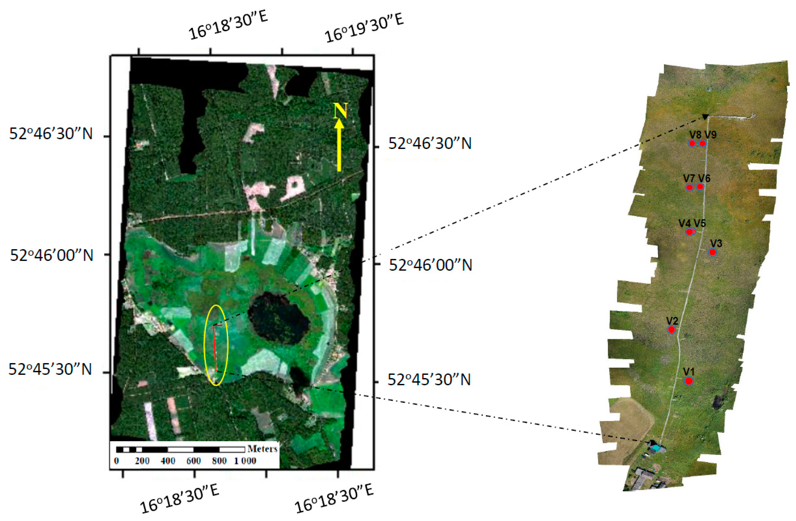
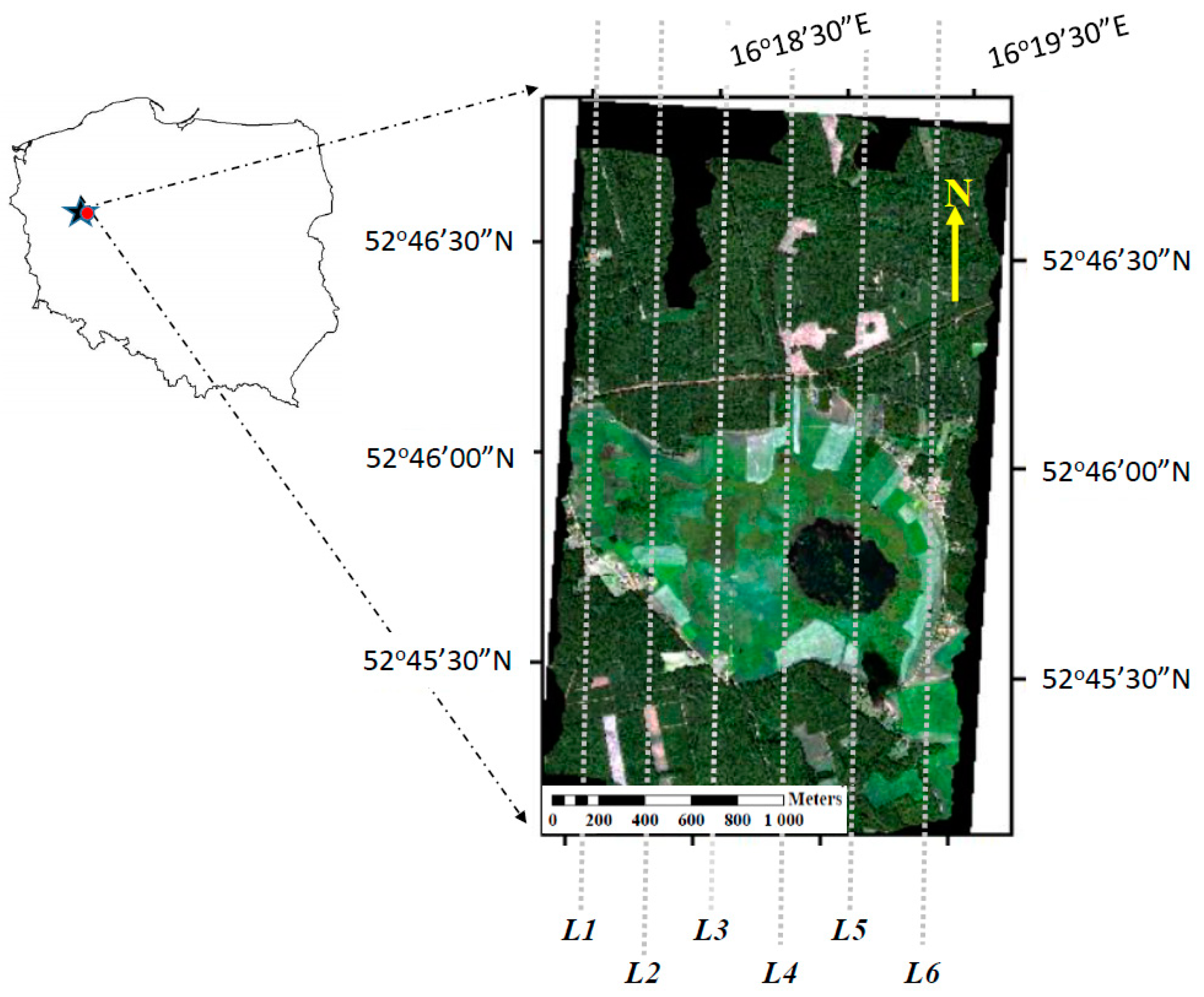
2.1. Site Description

This study was carried out in the Rzecin (POLWET) peatland area (Figure 1) located in western Poland (52°45′N, 16°18′E, 54 m asl). The whole Rzecin peatland, which is considered a poor fen, covers an area of 114 hectares [39]. According to historical and cartographic data, the peatland is a result of lake shallowing, a decelerated but ongoing process [39,40]. At the middle of the peatland, there is a station where measurements of greenhouse gas exchange (CO₂, CH₄, H₂O) have been carried out continuously since 2004 [41,42,43,44,45]. Geomorphologically, this peatland is located in between the dune areas of the Noteć Forest within the drainage basin of the Warta and Noteć rivers. The past 200 years of paleoecology history of the peatland is described in detail in Lamentowicz et al. [46].

The entire Rzecin peatland is extremely valuable from a floral and natural conservation perspective, and is included in the Natura 2000 network protected areas covering Europe’s most valuable and threatened species and habitats (“Torfowisko Rzecińskie” PLH300019 [47]). Different species of brown mosses, Sphagnum, and vascular plants (e.g., Eriophorum angustifolium, Carex lasiocarpa, Carex rostrata, Carex limosa, and Oxycoccus palustris) make this region eco-biologically unique [46,48]. In total, 127 species of vascular plants belonging to 43 families, and 34 taxa of mosses belonging to 10 families, were observed in this peatland area [48]. Among mosses, the most abundant moss species belong to Sphagnaceae and Amblystegiaceae. Twenty-six of the plant species found in Rzecin peatland are considered as rare and endangered at a regional-scale, while 20 species are locally endangered [48]. The annual mean air temperature of the study area is 8.3 °C, while the average annual precipitation sum is 530 mm (for 2004–2014).

2.2. Airborne Hyperspectral Measurements

Six flight lines were acquired between 09:50 to 10:46 and 13:10 to 13:55 on 11 July 2015, with HyPlant flying at an altitude of 690 m, resulting in a spatial resolution of 1 × 1 m per pixel. The measurements were acquired during cloud-free conditions. The HyPlant sensor, composed by the two push-broom sensors, was installed on a Cessna Grand Caravan C208B (a turboprop aircraft) owned and operated by CzechGlobe, Czech Republic. The first broadband dual-channel module (DUAL) was able to capture surface reflected radiance with a spectral resolution of 3 nm in the visible and near-infrared (VIS/NIR) regions, and about 10 nm in the short-wave infrared (SWIR) region, covering the total spectral domain between 370–2500 nm. The second narrow-band spectrometer (FLUO module) provided a high spectral resolution of 0.25 nm (Full Width at Half Maximum, FWHM) and quasi-continuously covered the red and far-red region of the electromagnetic spectrum ranges from 670 to 800 nm. The high-resolution FLUO module covered red and far-red regions of the electromagnetic spectrum, which allowed retrieving SIF close to the two atmospheric oxygen absorption bands O₂A (760 nm, F₇₆₀) and O₂B (687 nm, F₆₈₇).

The radiance images from DUAL and FLUO module were generated through a dedicated pre- and post-processing chain described in Colombo et al. [16] and Wieneke et al. [28]. Atmospheric and topographic corrections were carried out with the ATCOR (Atmospheric & Topographic Correction model, ReSe Applications Schläpfer, Langeggweg, Switzerland) to obtain Top-of-Canopy (TOC) reflectance and radiance values. Afterward, all the images were geo-rectified using CaliGeo toolbox (SPECIM, Oulu, Finland). Technical details about HyPlant, sensor calibration, image pre-processing, and post-processing, as well as sensor validation, are described in Rascher et al. [36].

2.3. Computation of Vegetation Indices

A number of reflectance-based narrowband VIs related to plant physiology, chemical composition, structure and water content were calculated from TOC reflectances obtained from the HyPlant DUAL-channel module (

Table 1. Vegetation indices calculated from HyPlant DUAL data. R in formulas represents the reflectance. Numbers refer to wavelengths in nm.

Vegetation Indices	Proxy	Formula	References
Simple Ratio (SR)	Greenness	$SR=\frac{R_{\langle 795-810\rangle }}{R_{\langle 665-680\rangle }}$	[49]
Normalized Difference Vegetation Index (NDVI)	Greenness	$NDVI=\frac{R_{\langle 795-810\rangle }-R_{\langle 665-680\rangle }}{R_{\langle 795-810\rangle }+R_{\langle 665-680\rangle }}$	[50]
Enhanced Vegetation Index (EVI)	Biomass	$EVI=2.5\left[\frac{R_{\langle 795-810\rangle }-R_{\langle 665-680\rangle }}{R_{\langle 795-810\rangle }+6·R_{\langle 665-680\rangle }-7.5·R_{\langle 475-490\rangle }+1}\right]$	[51]
Photochemical Reflectance Index (PRI)	xanthophyllcycle	$PRI=\frac{R_{\langle 570\pm 2.5\rangle }-R_{\langle 531\pm 2.5\rangle }}{R_{\langle 570\pm 2.5\rangle }+R_{\langle 531\pm 2.5\rangle }}$	[52]

). We mostly focused on greenness-related indices, such as normalized difference vegetation index (NDVI) and simple ratio (SR), as well as those related to biomass (enhanced vegetation index, EVI), photosynthesis, and xanthophyll cycle (photochemical reflectance index, PRI). PRI was calculated using the average of three spectral bands closest to 531 nm and 570 nm, respectively (center wavelength ±1 band), while the other indices were computed with spectral windows corresponding to 9 bands (center wavelength ±4 HyPlant spectral bands). From the TOC reflectance data, selected vegetation indices were calculated according to the equations provided in Table 1.

2.4. Retrieval of Sun-Induced Chlorophyll Fluorescence

The red and far-red fluorescence maps from the HyPlant sensor were computed based on the Spectral Fitting Methods (SFM) described in Cogliati et al. [53]. The retrieval algorithm, originally developed and tested for the FLEX mission, was further adapted for airborne observations. The algorithm used the high spectral resolution imagery detected by the HyPlant FLUO module. The technique relied on the analysis of the radiance spectra in high spectral resolution at the O₂ absorption bands (O₂-A and O₂-B at 760 and 687 nm, respectively), where the fluorescence contribution to the overall canopy emerging radiance was larger. The pre-processing steps consisted of the radiometric and spectral calibration, correction of detector non-linearity and the deconvolution of the instrument point-spread-function (PSF). The latter referred to the imagery processing technique used to remove stray-light (i.e., scattered light inside the spectrometer) caused by the optical elements of the instrument. In particular, the actual instrument PSF was characterized in the laboratory before the airborne survey and an adapted version of the Van-Cittert algorithm was applied. The fluorescence retrieval approach consisted of two main components: i) The atmospheric radiative transfer was computed through MODTRAN5 (MODerate resolution atmospheric TRANsmission) Radiative Transfer (RT) model; while ii) the decoupling of reflected and fluorescence radiances was achieved based on the spectral fitting technique. The atmospheric RT modelling and surface reflectance/fluorescence were coupled according to Verhoef et al. [54]. Basically, the retrieval was carried out at sensor-level, comparing the HyPlant and the forward-modelled radiance spectrum in defined spectral windows. The SFM algorithm was adapted considering the specific technical characteristics of HyPlant, exploiting the full set of spectral bands available around the oxygen absorption features. Specifically, the fluorescence retrieval at the O₂A and O₂B bands was achieved independently, considering two separate spectral windows (a few tens of nanometers wide) centered around the main absorption features. In particular, the SFM module implemented for HyPlant relied on third-order polynomial and pseudo-Voigt functions to approximate reflectance and fluorescence spectral behavior, respectively. As described in [53], the pseudo-Voigt function (i.e., weighted linear combination of a Lorentzian and Gaussian) is a convenient approach to approximate the computationally demanding Voigt function and thus limiting the over-processing time to retrieve fluorescence.

The atmospheric parameters required to run MODTRAN5 simulations were derived from Microtops II sunphotometer (Solar Light Company, Inc. Glenside, PA, USA ) measurements collected simultaneously to the airborne survey. A semi-automated script was developed for facilitating the extraction of sun-photometer measurements collected simultaneously with airborne imagery. Conversely, to most of the other retrieval techniques such as 3FLD [18,55] and iFLD [56], this semi-physically-based algorithm does not require reference surfaces within the image scene to constrain the atmospheric radiative transfer modelling (i.e., bare soil or other non-fluorescence pixels). On the other hand, the accuracy of such a physical approach depended on the overall quality of the atmospheric input parameters.

2.5. Top-of-Canopy Spectral Measurements of Reflectance and Sun-Induced Fluorescence

TOC spectral radiances were collected on 11 July 2015 at midday from 11:00 to 14:20 solar time under clear sky conditions at nine plots (V1–V9) located along the main boardwalk in S-N direction and representing different vegetation—i.e., from Carex and Typha (high biomass of vascular plants) to Sphagnum (low biomass of vascular plants) dominated groups (Figure 2,

Table 2. Detailed description of the validation plots (V1 to V9) with the corresponding coordinates, dominant species, Leaf Area Index (LAI) of vascular plants, and fraction of photosynthetically active radiation absorbed by plant canopy (fAPAR).

Target	Coordinates	Dominant Species	LAI * (m2 m−2)	fAPAR * (−)
V1	52.75933°N 16.30989°E	Carex gracilis	4.8 ± 0.5	0.93 ± 0.03
V2	52.76022°N 16.30969°E	Carex lasiocarpa, Menyanthes trifoliata, Oxycoccus palustris, Equisetum fluviatile, Sphagnum teres	1.7 ± 0.5	0.68 ± 0.19
V3	52.76067°N 16.30986°E	Typha latifolia, Carex rostrata, Lycopus europaeus, Lythrum salicaria, Calliergonella cuspidata, Drepanocladus polycarpos, Sphagnum teres	0.8 ± 0.4	0.18 ± 0.09
V4	52.76086°N 16.30975°E	Carex rostrata, Comarum palustre, Menyanthes trifoliata, Sphagnum angustifolium, Sphagnum teres	1.4 ± 0.4	0.20 ± 0.12
V5	52.76086°N 16.30975°E	Carex rostrata, Comarum palustre, Menyanthes trifoliata, Sphagnum angustifolium, Sphagnum teres	1.4 ± 0.4	0.20 ± 0.12
V6	52.76136°N 16.30969°E	Sphagnum teres, Carex rostrata, Comarum palustre, Drosera rotundifolia	0.9 ± 0.3	0.12 ± 0.07
V7	52.76136°N 16.30969°E	Carex rostrata, Comarum palustre, Sphagnum angustifolium	1.0 ± 0.3	0.16 ± 0.07
V8	52.76178°N 16.30964°E	Sphagnum teres, Carex rostrata, Oxycoccus palustris, Drosera rotundifolia	0.4 ± 0.1	0.06 ± 0.04
V9	52.76178°N 16.30964°E	Sphagnum teres, Carex rostrata, Oxycoccus palustris, Sphagnum angustifolium,	0.4 ± 0.1	0.06 ± 0.04

* LAI measured by means of SunScan system (Delta-T Devices, Cambridge, UK). fAPAR calculated as a ratio between Absorbed Photosynthetically Active Radiation (APAR) and incident Photosynthetically Active Radiation (PAR_i). APAR calculated as a difference between PAR_i and a sum of PAR transmitted trough the canopy and PAR reflected from the canopy. All PAR values measured by SunScan system.

).

The two spectrometers (HR4000, OceanOptics, Largo, FL, USA) covering different wavelength ranges were used to obtain TOC reflectance and SIF. One spectrometer operated in the visible and near-infrared (350–1050 nm) spectral range with a FWHM of 1 nm, suitable for computation of incident irradiance, visible to near-infrared reflectance, and VIs. The other spectrometer covered the 650–840 nm spectral range with a spectral resolution of 0.2 nm (FWHM) and was designed particularly for the estimation of SIF in the oxygen absorption bands O₂-A and O₂-B positioned at 760 nm (F760) and 687 nm (F687). Both spectrometers were housed in a Peltier thermally regulated box (model NT-16, Magapor, Zaragoza, Spain), keeping the internal temperature at 25 °C in order to reduce dark current drift (i.e., changes of the instrument noise level caused by temperature variations) [57]. The spectrometers were spectrally calibrated with known standards (CAL-2000 mercury argon lamp, OceanOptics, Largo, FL, USA), while the radiometric calibration was inferred from cross-calibration measurements performed with a reference calibrated FieldSpec spectrometer (Analytical Spectral Device, Boulder, CO, USA). Bare fiber optics with a field of view (FOV) of 25° were used to measure a white reference calibrated panel (Labsphere Inc., North Sutton, NH, USA) and the vegetated targets. To facilitate these measurements, the fibers were mounted on the tripod. The manual rotation of the mast allowed sequential measurements over the white reference panel and the vegetated targets [for details, see 23]. The targets were measured from nadir at a distance of 100 cm, corresponding to a sampling area of about 40 cm in diameter.

Five measurements over each plot were recorded and then averaged to reduce the noise in the sample. Spectral VIs indicated in Table 1 were calculated from TOC reflectance spectra. The fluorescence was estimated in the red and far-red regions (F₆₈₇ and F₇₆₀) using the spectral fitting methods (SFM) introduced by Meroni and Colombo (2009) [57] and Meroni et al. [58], and optimized by Cogliati et al. [53]. The spectral interval used for F₇₆₀ estimation was set in between 759.00 to 767.76 nm for a total of 439 spectral channels, while the spectral range between 684.00 and 696.00 nm for a total of 200 spectral channels was used for estimating the F₆₈₇.

2.6. Calibration and Rescaling of the HyPlant Fluorescence Maps

The accurate modelling of the atmospheric RT component inside the spectral fitting retrieval scheme is fundamental to achieve accurate and realistic fluorescence maps. In fact, uncertainties in atmospheric modelling rapidly propagate to the final fluorescence products, introducing significant discrepancies between airborne estimates in comparison with ground-based measurements. For this reason, we tested the possibility of re-calibrating the HyPlant fluorescence maps based on ground-based SIF measurements collected simultaneously in nine locations distributed from the edge to the middle of the peatland and representing different vegetation types, from vascular (at the edge of the peatland) to moss (in the middle) dominated groups (see Section 2.3).

Ground-based measured SIF at the plot-scale (Table 2, Figure 2) was compared with HyPlant measured SIF at both 687 nm and 760 nm. Hyplant-derived SIF and VIs values were calculated as an average of nine pixels (3 × 3) centered around each ground plot. Then, we tested a 1:1 linear regression model between SIF values computed from HyPlant and ground-based data and evaluated the strength of the correlation between SIF values for both chlorophyll fluorescence peaks at 687 nm (R² = 0.92) and 760 nm (R² = 0.87). The high correlation provided evidence that HyPlant-derived SIF can be rescaled to obtain more accurate SIF maps in absolute terms. It is important to note that the applied procedure did not change relative SIF spatial patterns across the whole image. This approach also facilitated a needed validation of obtained HyPlant SIF maps.

In order to rescale the SIF data retrieved from HyPlant, we processed each single pixel value of SIF within the whole SIF map based on the equation below:

$$SI{F}_{HyPlant\_corrected}=SI{F}_{HyPlant}·a+b$$

(1)

Due to specific features of the studied area and occurrence of the shallow lake in the middle of the peatland, around 10% of rescaled pixels were still negative. These negative pixels were set to zero for the purpose of getting the final SIF_{HyPlant_corrected} maps expressed in positive scales. The same procedure was applied to SIF maps derived at 687 and 760 nm.

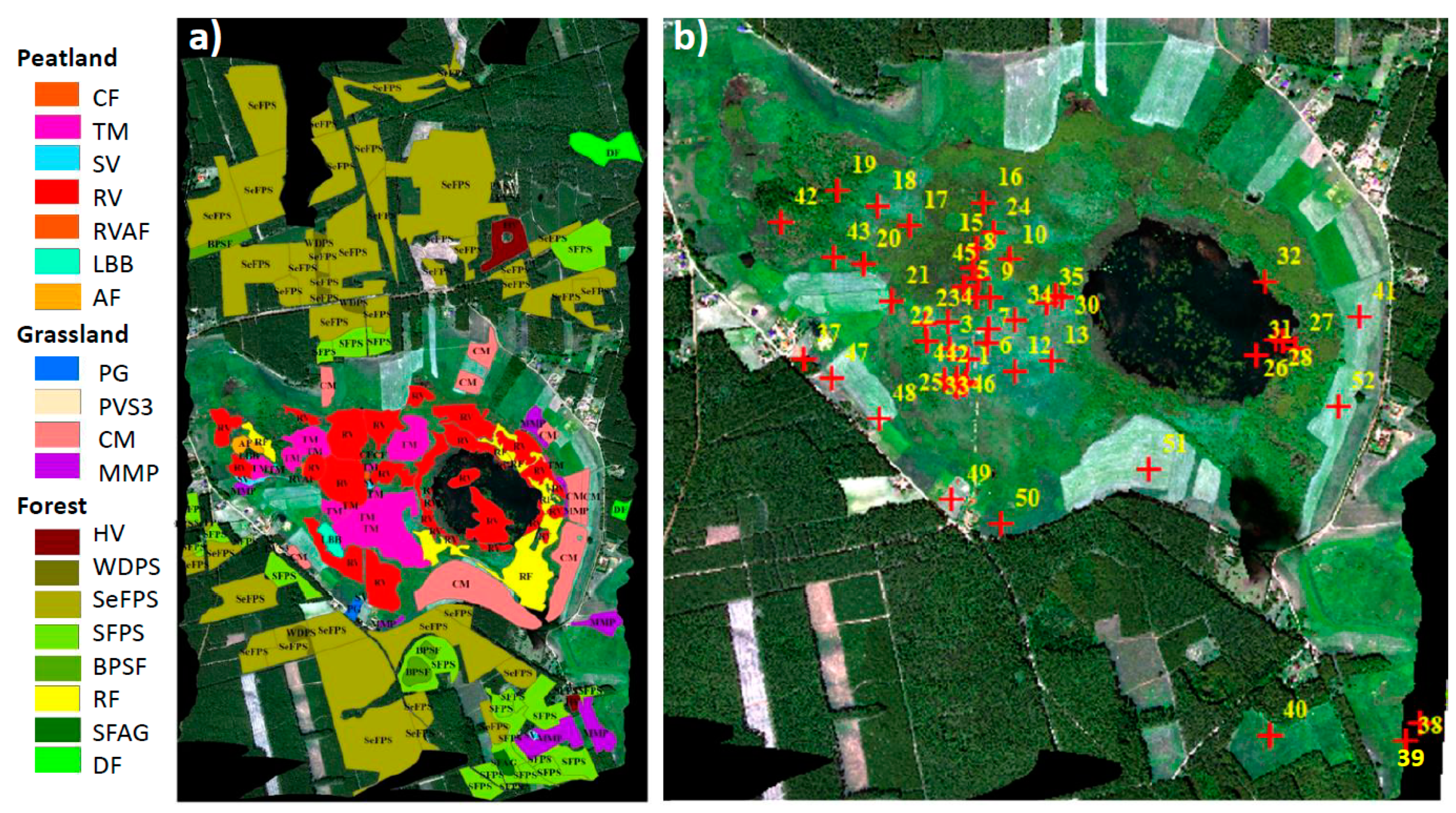
2.7. Identification of Vegetation Groups and Peatland Plant Communities

Regions of interest (ROIs) were defined to facilitate analyzing obtained spectral vegetation products and SIF signals for diverse vegetation groups representing peatland, forest, and grassland ecosystems, as well as peatland plant communities found in and around the peatland area. ROIs calculation was performed using ENVI 5.3 (Exelis VIS, Boulder, CO, USA) and ArcGIS 10.4 (Esri, Redlands, CA, USA). Selection of ROIs was based on the detailed vegetation survey. Vegetation surveys counted the dominant vegetation species and other plant species in the Rzecin peatland between 2014–2017. Areas without any vegetation survey background were not analyzed in the study.

Two different approaches were applied to assess RS information from the area of interest. In the first approach, the big area (forest, peatland, and grassland) of vegetation plant community in Rzecin (Poland) was considered. In the second approach, the small areas described as plots inside the heterogeneous peatland were considered.

For the first approach, we defined 158 ROIs with different shapes and sizes that were distributed over the whole site and covered with HyPlant. These 158 ROIs were subsequently categorized into 19 vegetation groups, considering three major ecosystem types: (i) Forest, (ii) grassland, and (iii) peatland. The spatial distribution and detailed names of the 19 vegetation groups are shown in Figure 3a.

For the second approach (i.e., the assessment of VIs and SIF for highly complex plant community patches inside the peatland area), we chose 52 individual plots. For these plots, a detailed botanical survey was done after the SWAMP campaign in the years of 2015–2017. The plots were selected by botanists to ensure that the most important plant communities of this peatland were covered. Each plot had an area of 25 square meters (5 m × 5 m). Vegetation cover (%) was recorded for the plots and later transformed according to the Van der Maarel scale [59] to categorize the most dominant species for that particular plot (1 = 0.5%, 2 = 0.5–1.5%, 3 = 1.5–3%, 4 = 3–5%, 5 = 5–12.5%, 6 = 12.5–25%, 7 = 25–50%, 8 = 50–75% and 9 = 75–100%). The plant communities were identified for each location according to the Braun-Blanquet method [60]. To reduce redundancy of a single plant community among the 52 locations, we integrated them into 20 unique plant communities, categorized into three major groups: (i) Meadows (ME), (ii) peatland rush (PR), and (iii) fen vegetation (FE). It must be noted that the lake area located inside the peatland was not considered in this study, and corresponding VIs and SIF values were masked and considered as non-value. Also, the floating vegetation and macrophytes over the lake area (plots 26–28, 31–32) were excluded from the analysis. Besides, there were two plots (38–39) located outside the image boundary. Hence the total number of plots used for the analysis of VIs and SIF was reduced to 46. A detailed description of the 52 individual plant communities with their associated locational IDs in Figure 3b is given in Table S1 (Supplementary Materials).

Legend a): (i) Forest vegetation groups: Herbaceous vegetation of forest clearings (HV); wooded dunes with Pinus sylvestris (WDPS); semi-natural forests with Pinus sylvestris (SeFPS); secondary forest communities with Pinus sylvestris (SFPS); Betula pendula–secondary forest communities (BPFS); riparian forests (RF); secondary forest communities with Alnus glutinosa (SFAG); deciduous forest (DF); (ii) Grassland vegetation groups: post-agriculture land (PG); pioneer vegetation of sandy and shallow soils (PVS3); mowed meadows and mesic pastures (CM); meadows and mesic pastures (MMP); (iii) Peatland vegetation groups: Calcareous fens (CF); transition mires (TM); sedge vegetation (SV); rush vegetation (RV); rush vegetation/alkaline fens (RVAF); low birch bush (LBB); alder forest (AF).

Legend b): (i) Meadows plant communities (ME): Agrostis capillaris-Hieracium pilosell (AP): 41; Mowed grassland (MG): 49, 51, 52; Semi mowed grassland (SMG): 48,50; Corniculario-Corynephoretum (CC): 37,47; Stellario palustris-Deschampsietum caespitosae (SPDC): 40; (ii) Peatland Rush communities (PR): Cladietum marisci (CM): 24; Phragmitetum communis (PC): 5,10,17,32; Caricetum lasiocarpae (CL): 1, 2, 11, 19, 25, 44, 46; Thelypterido-Phragmitetum (TP): 8; Typhetum latifoliae (TL): 30,43; (iii) Fen Vegetation communities (FE): Caricetum diandrae (CD): 21; Caricetum limosae (CLi): 14; Caricetum paniculatae (CP): 29,45; Caricion lasiocarpae (CLa): 13; Communities with dominated Sphagnum teres (CST): 16; Menyantho-Sphagnetum teretis (MST): 4; Sphagno apiculati-Caricetum rostrata (SACR): 3, 6, 7, 12, 15, 20, 22, 35; Sphagno recurvi-Eriophoretum angustifolii (SREA): 9, 18, 23, 34, 36; Sphagno-Caricetum rostrata (SCR): 42; Sphagnum teres (ST): 33.

2.8. Statistical Analysis

Extracted statistical values from the ROIs calculations over vegetation groups and peatland plant communities were used for statistical analysis. We employed bar plots, incorporating spatial variability through standard deviation (SD). Pearson’s correlation analysis was used to test the significance of the relationships between SIFs and VIs. Analyses were conducted for two different sets of data corresponding to small-scale plant communities identified for certain locations on the peatland and for big patches of areas covered with the same type of vegetation.

In order to determine if there are significant differences in relationships between SIFs and VIs, the two-sample t-test approach was applied. The differences between analyzed relationships were considered to be significant if the p-value obtained from the test was lower than 0.05. Statistical analysis was performed in non-commercial R studio (R Studio, Inc, Boston, MA, USA).

3. Results

3.1. Interpretation of VIs and SIF for Different Vegetation Groups

From the TOC reflectance data of HyPlant DUAL, we calculated several VIs maps as presented in Figure 4. The SR (Figure 4a) and NDVI (Figure 4b), which act as a proxy for vegetation greenness content, showed wide range of values between 0 to 56 and 0 to 0.96, respectively, over the study area [49,50] (Figure 4a,b). Grasslands and deciduous forest covers showed the highest values of SR and NDVI. Sparsely vegetated areas like post-agricultural land, pioneer vegetation of sandy and shallow soils, as well as herbaceous vegetation of forest clearings, showed significantly smaller values in both of the indices mentioned above.

EVI acts as a proxy of vegetation biomass, and also helps in the minimization of background signal and the atmospheric impact [51]. The derived EVI map (Figure 4c) showed comparatively higher values inside the peatland area due to the high density and biomass of the vegetation, whereas the smallest EVI values were recorded in forested areas surrounding the peatland. EVI ranged from 0 to 2.25, and the highest values of EVI were observed in extensive grassland areas located nearby the peatland. Xanthophyll cycle indicator PRI [52] was observed between a −0.43 to 0.30 range over the study area (Figure 4d). Higher values of PRI were observed from the peatland, whereas outer forest areas showed lower PRI values.

The maps provided in Figure 4e,f show the first SIF maps from a fen peatland. Maps of SIF₇₆₀ and SIF₆₈₇ from the Rzecin peatland represent novel and complementary information on the plant structure-function relationship. SIF₇₆₀ and SIF₆₈₇ for the heterogeneous peatland and its surroundings ranged between 0 to 3.21 mW·m⁻²·sr⁻¹ nm⁻¹ and 0 to 2.93 mW·m⁻²·sr⁻¹ nm⁻¹, respectively. Highest SIF emissions in both oxygen absorption bands (O₂A and O₂B) were obtained from grassland areas and deciduous forests, whereas non-fluorescent or very low-fluorescent targets like mowed grasslands, post-agricultural land, and herbaceous vegetation of forest clearings showed SIF values close to 0. A mixture of SIF signals was observed from both inside and outside of the peatland area.

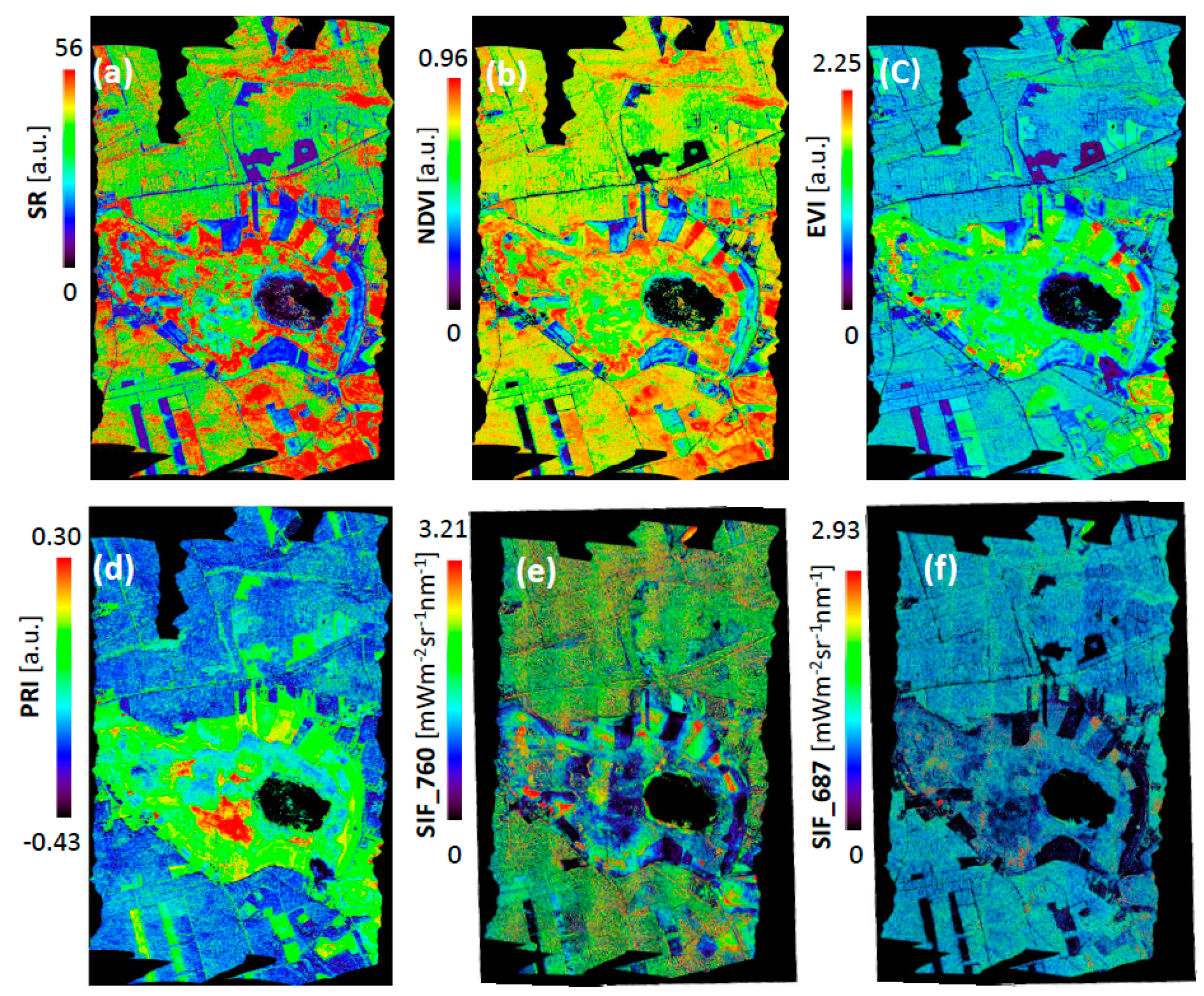
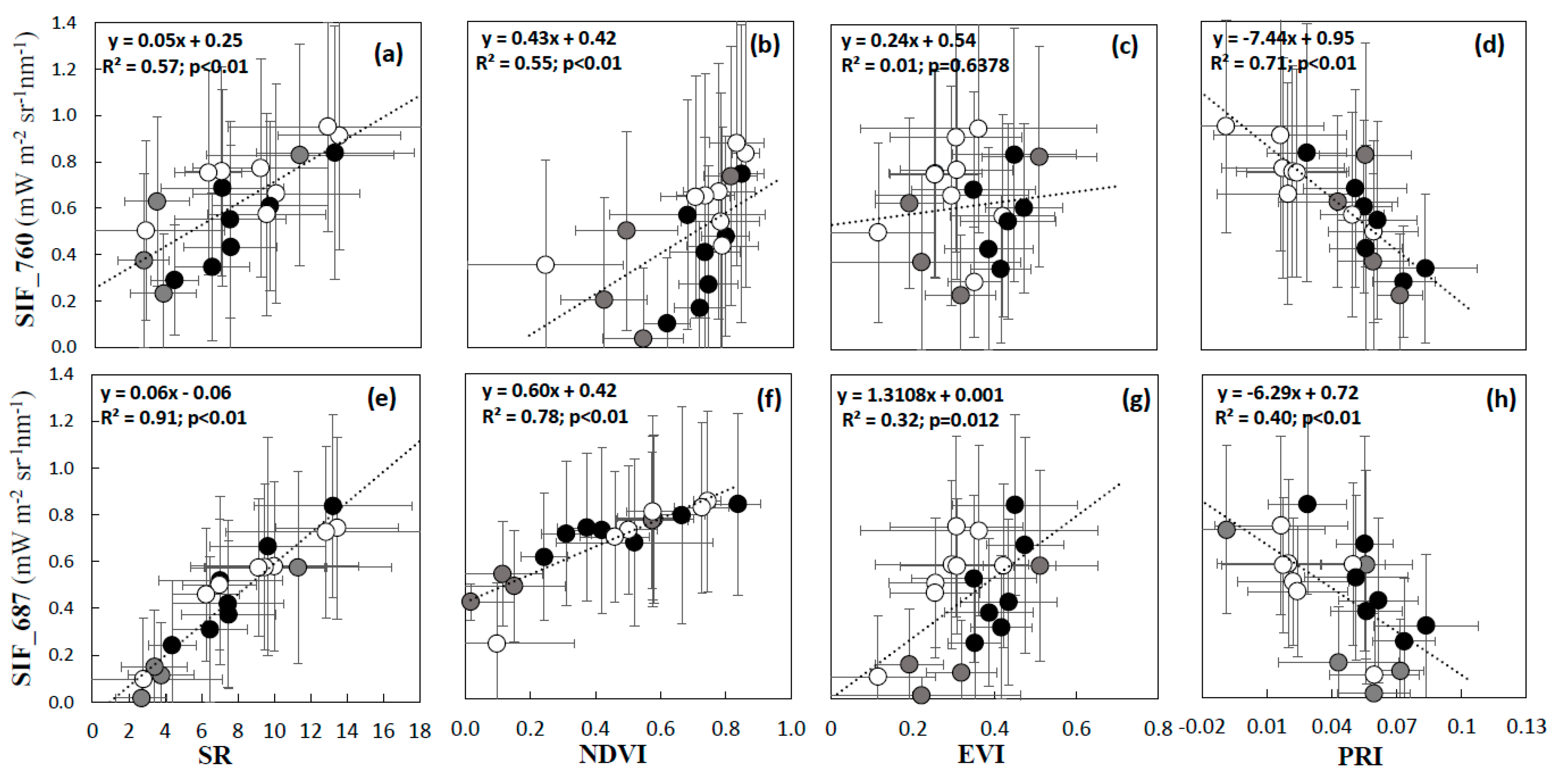
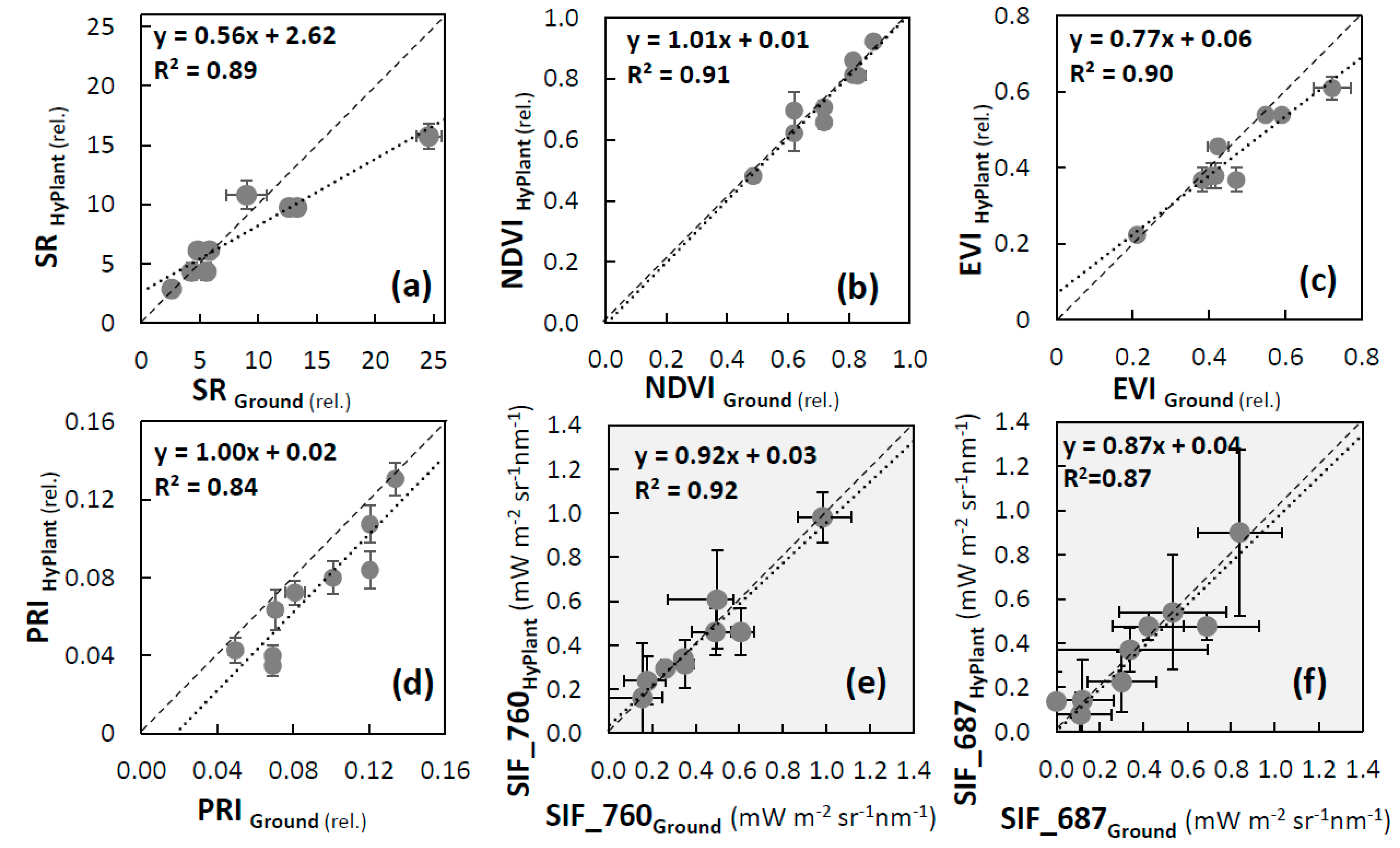
3.2. Validation of VIs and SIF Maps from HyPlant

The validation of airborne derived VIs and SIF was based on the comparison of HyPlant-derived VIs and SIF from DUAL and FLUO modules with simultaneously taken ground-based observations. HyPlant-derived vegetation products showed generally good agreement with the ground-based measurements (Figure 5a–d), with R² values of 0.89, 0.91, 0.90, 0.84 for SR, NDVI, EVI, and PRI, respectively. However, HyPlant-derived SR and EVI values were underestimated at the upper value range (i.e., above 6.0 and 0.4 for SR and EVI, respectively) and overestimated in the lower one. Large agreement between airborne and ground observation was found for NDVI, whereas PRI values were slightly underestimated in the whole range of the index values.

The HyPlant FLUO module derived TOC SIF values showed a strong correlation with ground-based measurements (Figure 5e,f). SIF showed a strong correlation in the red and far-red regions observed by the R² of 0.92 and 0.87 for SIF₇₆₀ and SIF₆₈₇, respectively. Higher values of SIF₇₆₀ and SIF₆₈₇ were observed for the Carex gracilis- and Carex lasiocarpa-dominated parts of the peatland (points V1–V2) at the outer zones, and then SIF signals become weaker towards the middle of the peatland and decreased with decreasing biomass of vascular plants, as indicated by lower Leaf Area Index (LAI) (see Figure 6 and Table 2). The lowest SIF values were observed at the Sphagnum-dominated parts of the peatland (V8–V9) where the LAI of vascular plants was the lowest (Table 2).

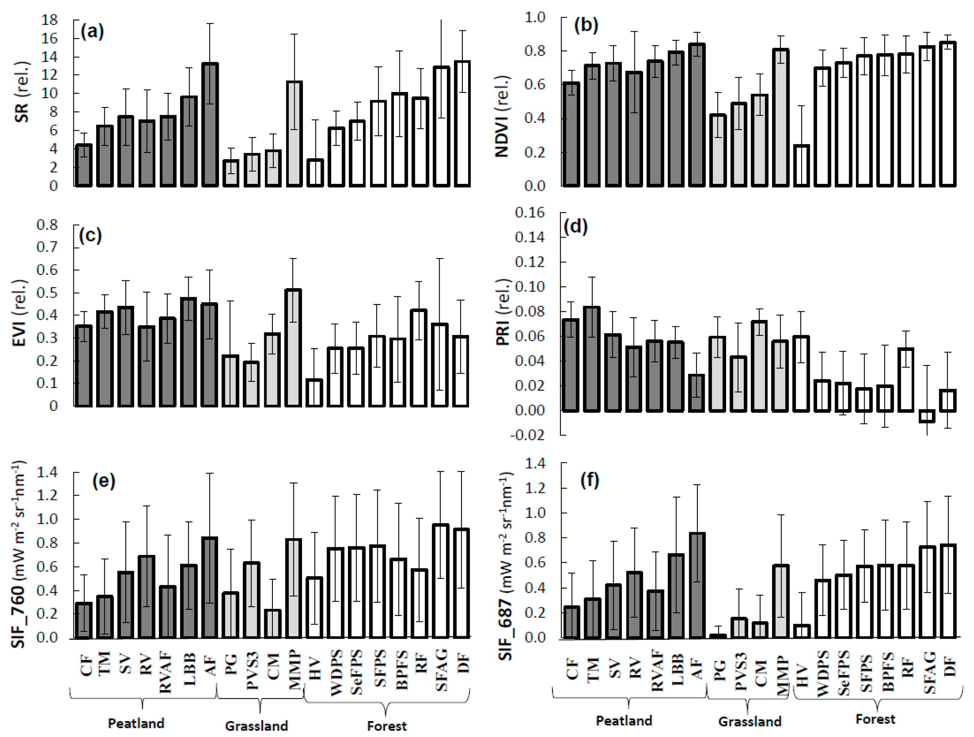
3.3. Analysis of VIs and SIF at Vegetation Group Level (for Peatland, Grassland, and Forest Ecosystems)

We explored vegetation information representing different plant traits (i.e., VIs and SIF) (Figure 7) considering peatland, grassland, and forest ecosystems. The dynamics of signals within particular vegetation groups were assessed to gain insight into biophysical, biochemical, and structural differences across vegetation types representing different ecosystems. The highest values of greenness-sensitive indices (i.e., SR, NDVI) were obtained for low birch bush (LBB) and alder forest (AF) due to their green leaves and dense canopies during the time of SWAMP campaign. Calcareous fens (CF) and transition mires (TM) showed the lowest values for greenness indices across peatland groups of vegetation since, due to the dominance of Sphagnum spp., their surface became whitish at the time of the campaign. Within the grassland group, the highest values of greenness indices were obtained for meadows and mesic pastures (MMP). Mowed meadows and mesic pastures (CM), in contrast, showed low values for greenness indices, possibly due to the low vegetation coverage in that area during the campaign time. Young deciduous forest (DF) and secondary forest communities with Alnus glutinosa (SFAG) were characterized by the highest greenness index values, whereas herbaceous vegetation of forest clearings (HV) showed the lowest values among the forest group.

A contrasting picture is obvious for the PRI: The highest PRI values were found for TM and CF, whereas PRI was lowest for AF within the peatland group. CM and HV showed the highest PRI signals, whereas MMP, SFAG, and young DF showed the lowest PRI signals within the grassland and forest groups, respectively.

Simultaneously, the highest to the lowest EVI signals were found for LBB, AF, and rush vegetation (RV), respectively, within the peatland group. Highest to lowest EVI are shown for MMP to CM, respectively, within the grassland group and riparian forests (RF), SFAG to the HV in the forest group, respectively.

The highest SIF₆₈₇ and SIF₇₆₀ values were found over LBB and AF within the peatland vegetation group; for MMP within the grassland group; and for SFAG and young DF (which is in agreement with Colombo et al. [16]) within the forest group. The lowest SIF signals in both O₂ absorption bands were recorded for CF and TM within the peatland group, for CM within the grassland group, and for HV within the forest group.

Positive relationships have been found for both SIF₆₈₇ and SIF₇₆₀ with both greenness indices SR and NDVI (Figure 8). At the same time, a negative relationship was observed between SIF and PRI. Relationships between SIF₇₆₀ and SIF₆₈₇ with NDVI, SR, and PRI were found to be statistically significant (p < 0.01) at the vegetation group level (Figure 8). However, a weak relationship was found between SIF₇₆₀ and EVI, although the correlation between SIF₆₈₇ and EVI was significant with p = 0.012.

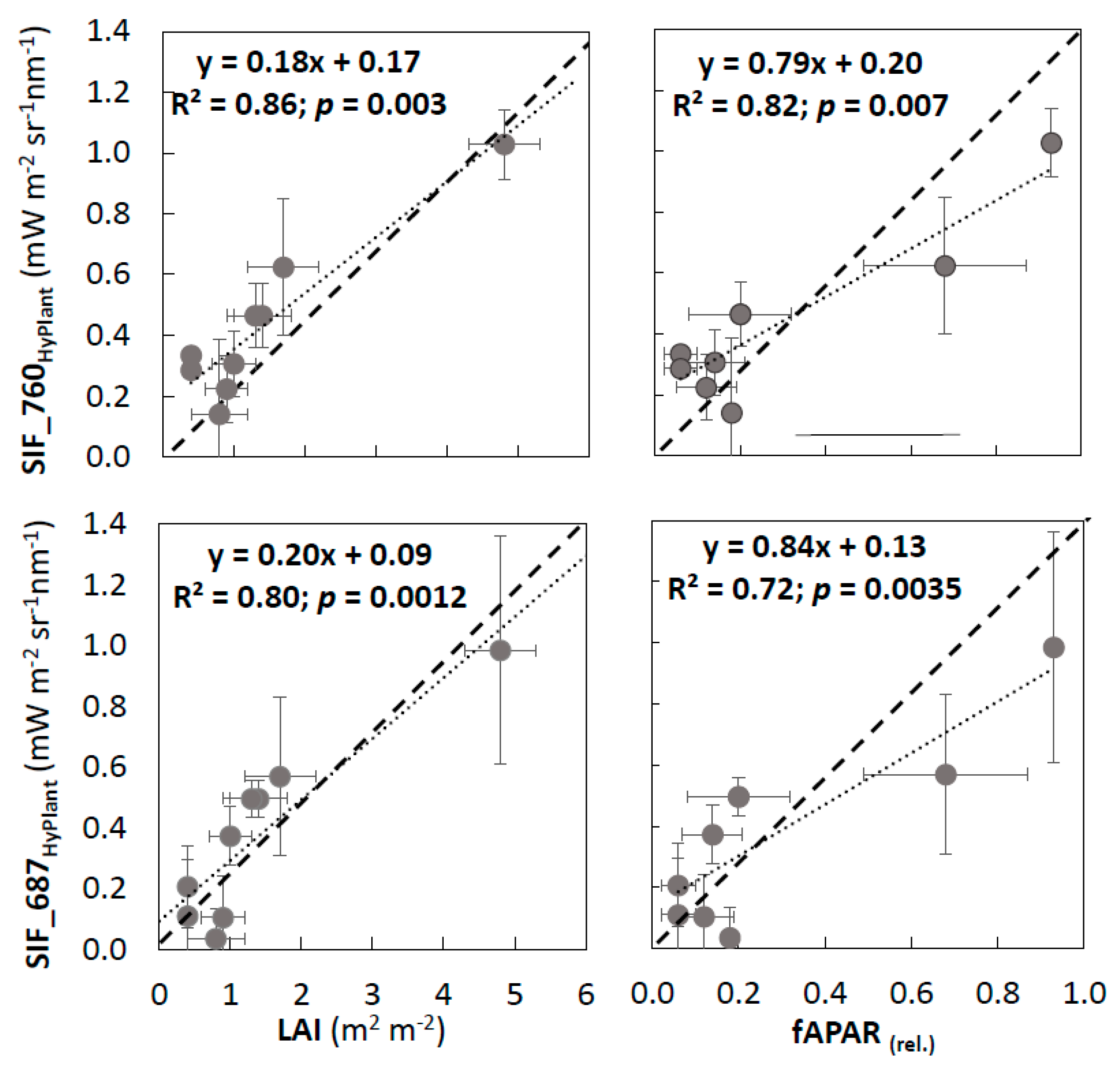
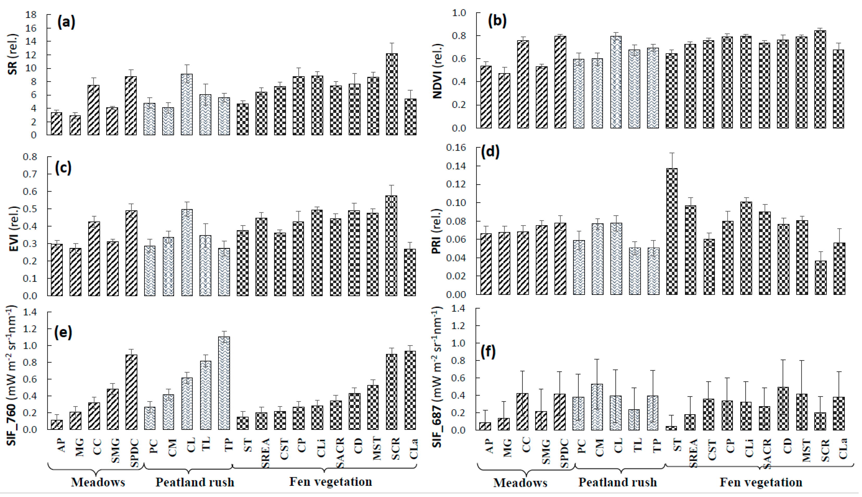
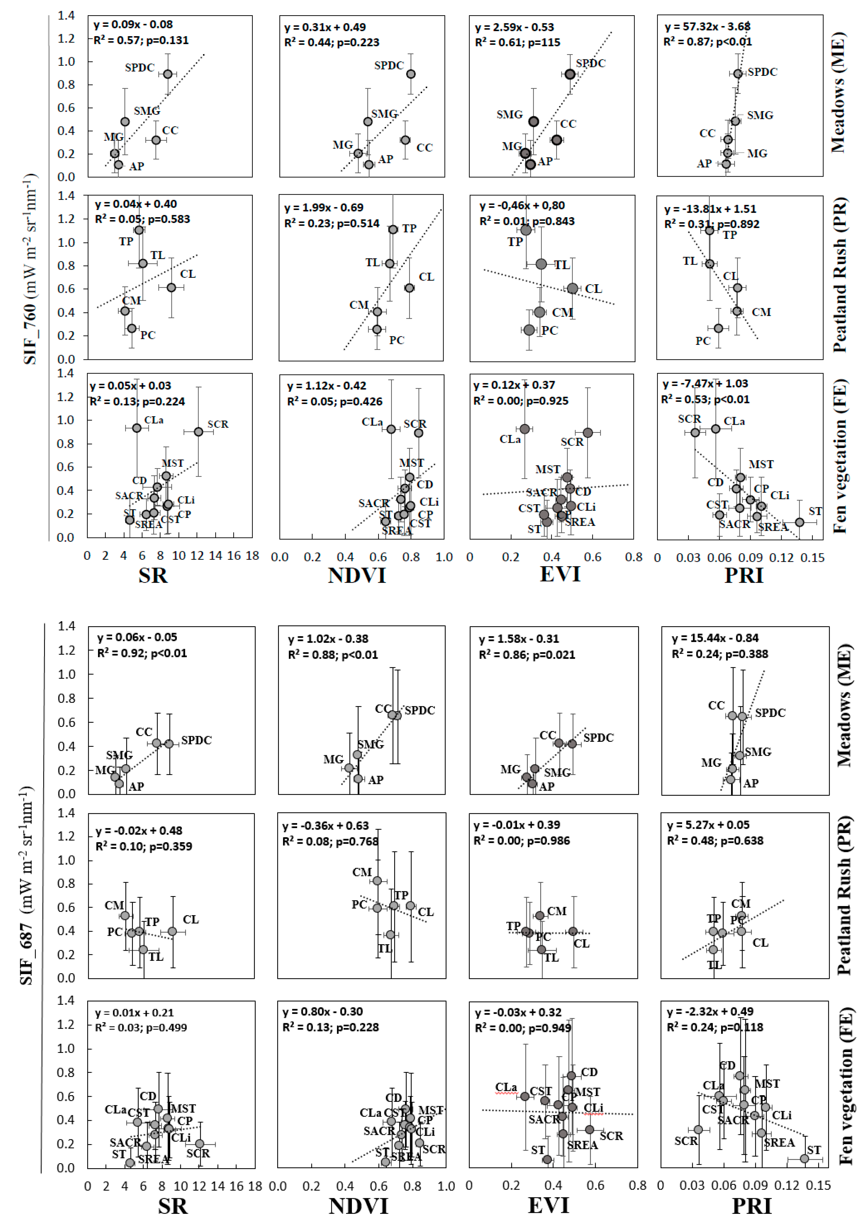
3.4. Performance of VIs and SIF Signals at the Peatland Plant Community Level

A wide range of VIs and SIF signals was observed for different peatland plant communities (see Figure 9), mainly due to their huge heterogeneity in terms of species richness, composition, dominance, structure of canopies, and functional variability. Due to this heterogeneity, the whole peatland plant community was categorized into three groups: i) Meadows (ME), ii) peatland rush vegetation (PR), and iii) fen vegetation (FE). ME represents the grasslands, whereas PR refers to several flowering peatland plants, and FE refers to the peatland mires. A detailed description of plant communities within the identified plant categories is provided in Table S1 (supplementary material). Among these three categories, ME were considered as spatially homogeneous patches of vegetation, whereas PR and FE vegetation groups reflect the heterogeneous nature of peatlands typically composed of many different species. According to the spatial coverage of our peatland site, PR and FE vegetation groups occupied the largest area of the peatland (90%) in contrast to meadows (10%) located at the edge of the peatland.

Figure 9 shows that within different peatland plant categories (ME, PR, and FE), each plant community was very individual and was characterized by unique values of VIs and SIF. The plant communities—like CC and SPDC from the ME category, CL from PR, and SCR from the FE category—showed the highest values of SR and NDVI. Whereas, MG and AP from the ME category, and CM and PC from the PR category, showed the lowest values of SR and NDVI. Similarly, ST and CLa within the FE category also showed the lowest values of SR and NDVI. The highest EVI was observed for SPDC, CL, and SCR in the ME, PR, and FE categories, respectively. Whereas, MG, TP, and CLa showed the lowest EVI in the ME, PR, and FE categories, respectively. In the ME category, all five plant communities were found to have almost similar PRI values. Whereas, CM and CL were found to have the highest PRI values under the PR category. Within the whole analyzed peatland plant communities, the highest PRI values were found for ST, and the lowest PRI values were observed for TL and TP within the PR community and SCR within the FE community.

All the plant communities within each group of vegetation (ME, PR, and FE) were sorted according to SIF₇₆₀ for clear visualization of the data in Figure 9. SPDC, TP, and CLa were recorded with the highest SIF₇₆₀, whereas AP, PC, and ST were recorded with the lowest SIF₇₆₀ in the ME, PR, and FE categories, respectively. The highest and the lowest SIF₆₈₇ signals in the ME category were observed for SPDC, CC, and AP, respectively. CM and CD were observed to have the highest SIF₆₈₇ values, whereas TL and ST the lowest within PR and FE categories, respectively.

To understand relationships between SIF and VIs at the narrower plant community-scale, from homogeneous meadows to heterogeneous rush and peatland vegetation, we assessed the 1:1 linear correlation between selected VIs and SIF within each vegetation category (Figure 10). In the ME category, relationships between SR, NDVI, EVI, and PRI with SIF₇₆₀ and SIF₆₈₇ were positive with R² ranging from 0.57 to 0.92 for SR, from 0.44 to 0.88 for NDVI, from 0.61 to 0.86 for EVI, and from 0.24 to 0.87 for PRI. Besides for PRI-SIF₆₈₇, SR-SIF₇₆₀, NDVI-SIF₇₆₀, and EVI-SIF₇₆₀, the rest of the investigated relationships were significant at p < 0.05. No such clear trends and strong relationships between VIs and SIF were found for heterogeneous vegetation groups of PR and FE. For both the PR and FE categories, relationships between SIF₇₆₀ and greenness indices (i.e., SR and NDVI) were also positive, but the R² ranged between 0.05 and 0.23 for SR and NDVI and was not statistically significant. Surprisingly, the same relationships of greenness indices with SIF₆₈₇ were negative for PR (although non-significant). The relationship between EVI and SIF₇₆₀ was weak and insignificant with R² = 0.01, p < 0.834 for the PR category and R² = 0.00, p < 0.925 for the FE category. Similarly, the relationship between EVI and SIF₆₈₇ was also very poor and insignificant for both the PR and FE categories.

In contrast to ME, the relationships between PRI and SIF₇₆₀ was negative for the PR and FE categories with R² from 0.31 to 0.53 for PR and FE, respectively; whereas, the relationships of PRI with SIF₆₈₇ were positive and insignificant for the PR (with R² = 0.48, p < 0.64), as well as negative and insignificant for the FE (with R² = 0.24, p < 0.12), vegetation categories.

4. Discussion

4.1. Reliability of SIF Retrievals and Vegetation Information

For the first time, SIF was retrieved in validated physical units along with various plant traits over a complex and heterogeneous peatland and its surroundings. Ground-based validation of airborne products indicated a good accuracy of retrieved vegetation information (Figure 5). Around 10% of the pixels expressed in negative SIF values (these pixels mostly represented the lake area and roads) were excluded from analyses, so they did not impact our results. Similar to Wieneke et al. [28], we observed higher noise in retrieved SIF maps compared to the VIs maps. Apparent noise effects, however, did not impact our analysis and interpretation. The highest variability (wide variability in signals observed in the map) of SIF₇₆₀ and SIF₆₈₇ was found for young deciduous forest, grassland, and alder forest areas in the studied vegetation sites, which is in agreement with Colombo et al. [16] (for forest), as well as Rossini et al. [37] and Gerhards et. al. [38] (for grasslands). Mowed grassland and cleaned forest areas showed the lowest SIF₇₆₀ and SIF₆₈₇ signals due to the low amount of photosynthetically-active plant tissue. For heterogeneous landscapes like peatlands, ground-based measurements are essential to assess the quality of RS derived information (as described by Calleja et al. [61]). That is why we put substantial efforts into the acquisition of ground-based SIF and reflectance data close to the acquisition time of the airborne sensor.

4.2. Sensitivity Analysis of Vegetation Groups

Observed vegetation information (i.e., SIF and trait-sensitive VIs) showed a large heterogeneity in and around the peatland area (Figure 4 and Figure 7). VIs and SIF maps from the pine forest, grassland, and peatland sites showed a clear structural-functional relationship [36]. A visual comparison of obtained maps indicated that greenness indices, non-greenness indices, and SIF represented different patterns for different vegetation groups. Inside the peatland area, alder forest, and low birch bush were characterized by rich green biomass during July, as represented by high values of greenness-sensitive indices. NDVI values of deciduous forest, meadows, mesic pastures, and alder forest showed saturation at values around 0.8, which is in agreement with Rascher et al. [36]. Some of the less-vegetated areas (e.g., herbaceous vegetation of forest clearing zones and mowed grasslands) showed less green vegetation coverage during the campaign time. Peatland calcareous fens were characterized with less dense vegetation [62] and showed the lowest greenness index values. The EVI, sensitive to canopy structure [28] and vegetation biomass [51], performed best for the regions where the green biomass was high, like alder forest, meadows and mesic pastures, riparian forests, and secondary forest communities with Alnus glutinosa. Although not shown, EVI was significantly correlated with greenness indices at both vegetation group and plant species composition levels, which was in agreement with Rocha et al. [63]. Furthermore, it was observed that the regions with the high greenness index values, like the deciduous forest, secondary forest communities with Alnus glutinosa, meadows and mesic pastures, Alder forest, and low birch bush, were characterized by low PRI values. PRI is an indicator of the xanthophyll cycle activity, and it increases with a decrease in SIF signals, as shown by different studies [64,65,66]. A negative relationship between SIF and PRI was also confirmed by our data. PRI denotes that the vegetation groups such as mowed meadows and mesic pastures, post-agriculture land, and forest clearings with high PRI values may have a higher rate of xanthophyll cycle activity, and vice-versa conditions applied to vegetation groups with low PRI. Sometimes encroachment, grazing/burning, and alleviation are the main stressors to the plants [67], which might be the reason behind high PRI signals at the post-agriculture land, mowed meadows, and mesic pastures, as well as herbaceous vegetation of forest clearing zones. PRI is also known to negatively correlate with the ratio of carotenoids to chlorophyll pigment concentrations [68], which may also explain the lower PRI in these areas.

The HyPlant sensor offered a unique opportunity to track not only far-red O₂A band signals, but also to capture narrower red O₂B band signals [37]. In our study, we reported both SIF bands at 760 nm and 687 nm from peatland vegetation groups and plant communities. However, the study by Verrelst et al. [69] showed that red fluorescence—rather than far-red—to be more sensitive to describe plant physiological process and canopy net photosynthesis. Apart from this study, only a few recent studies such as Wieneke et al. [28], Rossini et al. [37], Cheng et al. [66], Goulas et al. [70], Joiner et al. [71], Louis et al. [72], and Middleton et al. [73] exploited both the red and far-red SIF signals, mainly for agriculture or forest areas; therefore, future investigations are necessary for different landscapes [16]. To the best of our knowledge, we are the first to explore both SIF signals for heterogeneous peatland ecosystems. In our study, the SIF signals varied from 0 to 3.21 and to 2.93 for SIF₇₆₀ and SIF₆₈₇, respectively, where SIF₇₆₀ appeared to be more sensitive than SIF₆₈₇ over the whole study area. According to Damm et al. [18,19], SIF₇₆₀ is sensitive towards structural and functional properties of photosynthetic light conversion in canopies. We can further assume that SIF₇₆₀ may originate from the deeper layer of the canopies. This was because of foliage which was having a high transmission in that particular spectral region, as also previously reported by Rascher et al. [36]. For the peatland vegetation, we found clear and significant (p < 0.007) relationship between SIF₇₆₀ and SIF₆₈₇ and fAPAR (Figure 6). Therefore, the results confirm that SIF can be considered as an excellent indicator of the amount of light absorbed by chlorophyll and used in photosynthesis (e.g., [36,37,74,75]) for a heterogeneous ecosystem like peatland.

High fluorescence values of the deciduous forest, secondary forest communities with Alnus glutinosa, meadows and mesic pastures, as well as alder forest, suggest that SIF reflects more than just greenness of the canopies. From the ground observation of vegetation during the time of the campaign, we confirmed that the deciduous trees were in their young stage, which was also shown by RS observation. Our finding was in agreement with Colombo et al. [16], where he showed a strong relationship between high SIF values and young age deciduous trees. In agreement with our study, Rossini et al. [37] have also observed a high SIF emission from densely covered grasslands. In our study, alder forest and low birch bush located inside the peatland area, as well as grasslands located at the edge of the peatland, were covered by the dense green canopies and were observed to be a source of high emission of both SIF₇₆₀ and SIF₆₈₇ signals during the campaign. However, low vegetative covers were observed to show a weak SIF signal, as well as low values of greenness indices.

The result also showed a significant positive relationship between two SIF bands with greenness indices. Different studies have demonstrated that reflectance-based VIs like NDVI have successively improved our understanding about global ecosystems by providing estimates of potential photosynthesis from greenness estimates [76,77,78]. Sometimes, NDVI is used to track the development of vegetation phenology, whereas SIF is considered to be a prime parameter to estimate GPP (e.g., [25,79]). Considering that we found significant relationships between SIF and NDVI at the vegetation group level, and positive relationships between SIFs and fAPAR (Figure 6), we can hypothesize that canopies with higher values of SIF and greenness VIs were more photosynthetically active during the campaign. Therefore, we can farther assume that SIF retrieved from Hyplant may reflect the spatial variability of GPP for these ecosystems (although not confirmed by measurements). The reflectance-based indices such as NDVI and SR are insufficient for the purpose of estimating the photosynthetic process, whereas SIF can be highly correlated with photosynthesis [80]. A study by Yang et al. [30] showed that at the initial stage, SIF₇₆₀ increases with chlorophyll content, whereas SIF₇₆₀ saturates at with high chlorophyll content due to the saturation of light absorption by chlorophyll molecules with the high chlorophyll content [30,81]. Our results showed that SIF₆₈₇, which is less sensitive to photosynthesis but does not easily get saturated, correlated highly with greenness indices, but also with EVI and PRI. These relationships were, however, weaker for SIF₇₆₀.

Some other reasons behind the good agreement between SIF and VIs for large vegetation patches may be: (1) Less quantity of mixed pixels, (2) the absence of mixed signals in dominant vegetation groups, and (3) less influence of microclimatic and local environmental stress factors. Another important reason can be related to the large dimension of the canopies and the changes in sunlight and shadow areas within the FOV, which plays a major role during the daytime and ultimately influences the signal of fluorescence emission (as described in Cogliati et al. [17]).

4.3. Sensitivity Analysis of Peatland Plant Communities

The results from Figure 9 have demonstrated the dynamics of VIs and SIF signals from heterogeneous peatland plant communities. The outputs were explored by the potential capability of the high-resolution HyPlant images to showcase the extracted VIs and SIF signals from small-scale homogeneous to heterogeneous peatland plant communities. No such studies to date have used the HyPlant hyperspectral imaging spectroscopy system to understand the dynamics of heterogeneous peatland plant community signals of VIs and fluorescence in both red and far-red regions. In a dynamic ecosystem like peatland, the spectral signatures of plants species, which represent the biodiversity of the peatland as well as the biophysical properties of vegetation cover, are very dynamic by nature [8]. Due to the frequent change of the environmental conditions, peatland plant species are continuously facing challenges for their survival, which ultimately impact their biophysical conditions and can be observed by the deviation in spectral reflectance [81]. This variation is not surprising, as the green leaves in the very short term (minutes, hours, days) remain green, but the photosynthesis decreases under stress condition [82]. Such kind of very dynamic situation may impact SIF-VIs relationships, particularly for peatland vegetation. Even the magnitude of the frequently changing rate of photosynthesis due to certain local stress factors—such as extreme temperature, direct sunlight, a temporary shortage of water, or nutrient content—may hamper the SIF-VIs agreement [83]. In the peatland ecosystem, water table depth plays a crucial role in the plants and determines the species composition of the peatland [81]. A slight drop or lift in water table may impact the vegetation functionality drastically and may also influence the SIF and VIs.

SPDC and CC in the ME category were perennial grasses with long canopy distribution, which are highly dependent on the soil moisture content [84,85]. In July 2015, these plant communities were in their full phase of growth, which was reflected by the higher values of greenness indices (SR, NDVI) and EVI. Also, values of SIF₆₈₇ were the highest for these communities, although SIF₇₆₀ was nearly three times higher for SPDC than for CC plant communities. At the same time, MG was suffering from low vegetation coverage during the campaign time, which explains the low value of greenness indices and both SIFs. Similarly, CL in the PR category and SCR in the FE category were tall and dense vegetation, represented by the highest values of greenness indices and one of the highest values of SIF₇₆₀. We observed the plant communities like SPDC in the ME category, CL in the peatland rush vegetation category, and SCR in the FE category all had higher EVI signals due to their high green biomass content. No such variation of PRI signals was observed in the ME category. ST in the FE category was observed with a very high PRI and the lowest SIF signals.

A clear gradient was observed in SIF₇₆₀ within the plant communities under different vegetation categories. For the vascular plant communities, high biomass could be the reason for higher SIF₇₆₀ signal. An increase in the biomass of vascular plants is known to accelerate the rates of photosynthesis [86]. In the homogeneous meadows category, poor AP to rich SPDC was observed with the lowest to highest SIF₇₆₀ emissions. For heterogeneous rush vegetation, coverage and dominance of some vascular plant species might be the main reason for the lowest to highest SIF₇₆₀ signal emission. Less covered and diverse PC emitted lower SIF₇₆₀, while highly dense and more species-rich TP emitted higher SIF₇₆₀. In the FE category, an abundance of vascular plant species might be a cause for the lowest to highest SIF₇₆₀ emission, too. The lowest SIF₇₆₀ signal originated from ST, characterized with very low abundance and biomass of vascular plants. Whereas, CLa, characterized by a higher abundance of vascular plants, provided high SIF signals. We did not observe any trend of similarity between SIF₆₈₇ and SIF₇₆₀ signals from different plant communities. Firstly, this might be due to less sensitivity for re-absorption of red-fluorescence at microscale plant community level [28]. Secondly, the probability of a mixture of signals from heterogeneous surfaces may also be a reason for lower sensitivity at a lower spatial scale [87].

In this study, we also showed the relationships between SIF and VIs for homogeneous and heterogeneous categories of peatland vegetation (fen, peatland rush, and meadows). From Figure 10, it is clear that for homogeneous meadows the relationships between SIF and VIs were positive and comparable to those determined based on a larger spatial scale of vegetation groups identified for different ecosystems. No such relation was observed, or they were just very poor and non-significant, for heterogeneous rush and peat vegetation communities. The impact of different vegetation species on such relationships may be strongly related to the type of peatland, such as the homogeneous or heterogeneous nature of the peatland [3]. The uniqueness of our study was that the Rzecin peatland consisted of both kind of surfaces, which were located in different parts of the peatland area. The homogeneous meadows were located in the periphery of the peatland, whereas heterogeneous rush and peatland vegetation was the most dominating vegetation group located inside of the peatland. Studies have shown that differences among vegetation types or the character of the peatland are influential enough to affect the vegetation relationship with spectral data (e.g., [3]). Thus, the chances of mixed pixel (in terms of the mixture of signals) obtained from peatland plant communities is higher in heterogeneous patches than a homogeneous ones. Small et al. [87] showed that mixed pixels might influence statistical classification methods because most algorithms are based on the assumption of spectral homogeneity at pixel-scale within a particular class of land cover. Thus, we can assume that due to the spectral homogeneity of meadows, the emitted SIF signals were not much disturbed, whereas in heterogonous fen and peatland rush vegetation groups the SIF signals were influenced by mixing, which ultimately impacted the correlation of VIs and SIF.

Our results indicate that SIF values did not increase with an increase in species diversity and species richness within the plant communities identified on the peatland. Higher values of SIF₇₆₀ were associated with a higher biomass of vascular plants with higher LAI (Figure 6). On the other hand, SIF₆₈₇ was less sensitive to changes in species richness and biomass of vascular plants. We can state, that SIF, especially SIF₇₆₀, was strongly associated with the functional diversity of peatland vegetation. Therefore, it was possible to identify the plant communities of high perennials, showing higher values of SIF₇₆₀ (associated with LAI > 5.0 m²·m⁻²). Whereas, lower values of SIF₇₆₀ indicated peatland patches dominated by Sphagnum spp., which are known to have lower productivity and lower coverage and LAI (<0.8 m²·m⁻²) of vascular plants (Table 2, Figure 6). In general, we can state that SIF reflects very well the productivity gradient on the fen peatland, from Sphagnum-dominated patches with the lowest SIF and the lowest fAPAR and productivity to the Carex-dominated patches with the highest SIF and higher fAPAR and productivity [74,75,88]. This specific feature of SIF can be potentially used in practice to monitor the peatland overgrowing processes caused by the succession of unfavorable reeds or other rush species due to ongoing degradation processes of the peatland.

5. Conclusions

Our results are the first experimental evidence of the possibility of retrieving both red (SIF₆₈₇) and far-red (SIF₇₆₀) chlorophyll fluorescence signals over heterogeneous ecosystems, such as peatlands. The reliability and capacity of a novel airborne HyPlant sensor were also demonstrated in this paper, which successfully captures complex vegetation signals from extremely heterogeneous peatlands. The results are valid for some specific conditions, and the status of the peatland is dependent on the hydrometeorological and climatological conditions related to the summer conditions. Hence, the findings cannot be extrapolated and may not be valid out of the season, when the status of the peatland, the greenness of the surface, and biomass of plants are different.

Although all the results of this study depend on one-day airborne measurement, the results have illustrated a promising method to understand the dynamic degree of relationships between SIF and VIs at different hierarchical scales using HyPlant, the airborne demonstrator of ESA FLEX mission. We conclude on the importance of hyperspectral RS information representing a diverse set of vegetation traits—including biochemical, structural, and functional traits—to comprehensively assess the complex ecosystems, such as peatlands, and to capture the wide diversity of different vegetation groups and peatland plant communities.

In such a complex ecosystem like peatlands, we suggest quantifying and analyzing red and far-red fluorescence peaks to improve our understanding and facilitate predictions of functional dynamics in larger vegetation groups and small plant community levels, which are determined by complex interplays between functional and structural regulations [89,90,91,92].

Comprehensive measurements of SIF, fAPAR, LAI, and VIs help in the advance estimations of photosynthesis activity, biochemical and structural traits, and facilitate assessments of the wide functional diversity of vegetation groups and plant communities occurring in such ecosystems. Since SIF is considered as a prime indicator of photosynthetic activity and is clearly correlated with fAPAR and LAI, we can assume that diversity in SIF maps reflects the diversity in their photosynthetic activity, which may correspond to photosynthesising biomass of vascular plants. Our results successfully support this claim for the first time in heterogeneous surfaces like peatlands. This may further enrich our knowledge on a local, regional, and global understanding of the photosynthetic activity of natural ecosystems.

References

1. Gorham, E. Northern peatlands: Role in the carbon cycle and probable responses to climatic warming. Ecol. Appl. 1991, 1, 182–195. [Google Scholar] [CrossRef] [PubMed]
2. Limpens, J.; Berendse, F.; Blodau, C.; Canadell, J.G.; Freeman, C.; Holden, J.; Roulet, N.; Rydin, H.; Schaepman-Strub, G. Peatlands and the carbon cycle: From local processes to global implications-a synthesis. Biogeosciences 2008, 5, 1475–1491. [Google Scholar] [CrossRef]
3. Lees, K.J.; Quaife, T.; Artz, R.R.E.; Khomik, M.; Clark, J.M. Potential for using remote sensing to estimate carbon fluxes across northern peatlands—A review. Sci. Total Environ. 2018, 615, 857–874. [Google Scholar] [CrossRef]
4. Holden, J.; Shotbolt, L.; Bonn, A.; Burt, T.P.; Chapman, P.J.; Dougill, A.J.; Fraser, E.D.G.; Hubacek, K.; Irvine, B.; Kirkby, M.J.; et al. Environmental change in moorland landscapes. Earth-Sci. Rev. 2007, 82, 75–100. [Google Scholar] [CrossRef]
5. Bonn, A.; Allott, T.; Hubacek, K.; Stewart, J.; Allott, T. Drivers of change in upland environments: Concepts, threats and opportunities. In Drivers of Environmental Change in Uplands; Bonn, A., Allott, T., Hubacek, K., Stewart, J., Eds.; Routledge: Abingdon, UK, 2009; pp. 1–10. [Google Scholar]
6. Van der Wal, R. Mountains, moorlands and heaths. In The UK National Ecosystem Assessment Technical Report; UNEP-WCMC: Cambridge, UK, 2011; Chapter 5. [Google Scholar]
7. Cole, B.; McMorrow, J.; Evans, M. Spectral monitoring of moorland plant phenology to identify a temporal window for hyperspectral remote sensing of peatland. ISPRS J. Photogramm. Remote Sens. 2014, 90, 49–58. [Google Scholar] [CrossRef]
8. Erudel, T.; Fabre, S.; Houet, T.; Mazier, F.; Briottet, X. Criteria Comparison for Classifying Peatland Vegetation Types Using In Situ Hyperspectral Measurements. Remote Sens. 2017, 9, 748. [Google Scholar] [CrossRef]
9. Mehner, H.; Cutler, M.; Fairbairn, D.; Thompson, G. Remote sensing of upland vegetation: The potential of high spatial resolution satellite sensors. Glob. Ecol. Biogeogr. 2004, 13, 359–369. [Google Scholar] [CrossRef]
10. Adam, E.; Mutanga, O.; Rugege, D. Multispectral and hyperspectral remote sensing for identification and mapping of wetland vegetation: A review. Wetl. Ecol. Manag. 2010, 18, 281–296. [Google Scholar] [CrossRef]
11. Yu, Z.C. Northern peatland carbon stocks and dynamics: A review. Biogeosciences 2012, 9, 4071–4085. [Google Scholar] [CrossRef]
12. Seher, J.S.; Tueller, P.T. Color aerial photos for marshland. Photogramm. Eng. 1973, 9. [Google Scholar]
13. Schmidt, K.S.; Skidmore, A.K. Spectral discrimination of vegetation types in a coastal wetland. Remote Sens. Environ. 2003, 85, 92–108. [Google Scholar] [CrossRef]
14. Guyot, G. Optical properties of vegetation canopies. In Applications of remote sensing in agriculture; Steven, M.D., Clark, J.A, Eds.; Butterworths: Kent, UK, 1990; pp. 19–43. [Google Scholar]
15. Drusch, M.; Moreno, J.; Del Bello, U.; Franco, R.; Goulas, Y.; Huth, A.; Kraft, S.; Middleton, E.M.; Miglietta, F.; Mohammed, G.; et al. The FLuorescence EXplorer Mission Concept—ESA’s Earth Explorer 8. IEEE Trans. Geosci. Remote Sens. 2017, 55, 1273–1284. [Google Scholar] [CrossRef]
16. Colombo, R.; Celesti, M.; Bianchi, R.; Campbell, P.K.; Cogliati, S.; Cook, B.D.; Corp, L.A.; Damm, A.; Domec, J.C.; Guanter, L.; et al. Variability of sun-induced chlorophyll fluorescence according to stand age-related processes in a managed loblolly pine forest. Glob. Chang. Biol. 2018, 24, 2980–2996. [Google Scholar] [CrossRef] [PubMed] [Green Version]
17. Cogliati, S.; Rossini, M.; Julitta, T.; Meroni, M.; Schickling, A.; Burkart, A.; Pinto, F.; Rascher, U.; Colombo, R. Continuous and long-term measurements of reflectance and sun-induced chlorophyll fluorescence by using novel automated field spectroscopy systems. Remote Sens. Environ. 2015, 164, 270–281. [Google Scholar] [CrossRef]
18. Damm, A.; Elbers, J.A.N.; Erler, A.; Gioli, B.; Hamdi, K.; Hutjes, R.; Kosvancova, M.; Meroni, M.; Miglietta, F.; Moersch, A.; et al. Remote sensing of sun-induced fluorescence to improve modeling of diurnal courses of gross primary production (GPP). Glob. Chang. Biol. 2010, 16, 171–186. [Google Scholar] [CrossRef]
19. Damm, A.; Guanter, L.; Paul-Limoges, E.; van der Tol, C.; Hueni, A.; Buchmann, N.; Eugster, W.; Ammann, C.; Schaepman, M.E. Far-red sun-induced chlorophyll fluorescence shows ecosystem-specific relationships to gross primary production: An assessment based on observational and modeling approaches. Remote Sens. Environ. 2015, 166, 91–105. [Google Scholar] [CrossRef]
20. Guanter, L.; Zhang, Y.; Jung, M.; Joiner, J.; Voigt, M.; Berry, J.A.; Frankenberg, C.; Huete, A.R.; Zarco-Tejada, P.; Lee, J.E.; et al. Global and time-resolved monitoring of crop photosynthesis with chlorophyll fluorescence. Proc. Natl. Acad. Sci. USA 2014, 111, E1327–E1333. [Google Scholar] [CrossRef] [PubMed] [Green Version]
21. Zhang, Y.; Joiner, J.; Alemohammad, S.H.; Zhou, S.; Gentine, P. A global spatially contiguous solar-induced fluorescence (CSIF) dataset using neural networks. Biogeosciences 2018, 15, 5779–5800. [Google Scholar] [CrossRef] [Green Version]
22. Joiner, J.; Yoshida, Y.; Vasilkov, A.P.; Schaefer, K.; Jung, M.; Guanter, L.; Zhang, Y.; Garrity, S.; Middleton, E.M.; Huemmrich, K.F.; et al. The seasonal cycle of satellite chlorophyll fluorescence observations and its relationship to vegetation phenology and ecosystem atmosphere carbon exchange. Remote Sens. Environ. 2014, 152, 375–391. [Google Scholar] [CrossRef] [Green Version]
23. Rossini, M.; Meroni, M.; Celesti, M.; Cogliati, S.; Julitta, T.; Panigada, C.; Rascher, U.; van der Tol, C.; Colombo, R. Analysis of red and far-red sun-induced chlorophyll fluorescence and their ratio in different canopies based on observed and modeled data. Remote Sens. 2016, 8, 412. [Google Scholar] [CrossRef]
24. Zhang, Y.; Guanter, L.; Berry, J.A.; van der Tol, C.; Yang, X.; Tang, J.; Zhang, F. Model-based analysis of the relationship between sun-induced chlorophyll fluorescence and gross primary production for remote sensing applications. Remote Sens. Environ. 2016, 187, 145–155. [Google Scholar] [CrossRef] [Green Version]
25. Migliavacca, M.; Perez-Priego, O.; Rossini, M.; El-Madany, T.S.; Moreno, G.; van der Tol, C.; Rascher, U.; Berninger, A.; Bessenbacher, V.; Burkart, A.; et al. Plant functional traits and canopy structure control the relationship between photosynthetic CO 2 uptake and far-red sun-induced fluorescence in a Mediterranean grassland under different nutrient availability. New Phytol. 2017, 214, 1078–1091. [Google Scholar] [CrossRef] [PubMed]
26. Parazoo, N.C.; Bowman, K.; Fisher, J.B.; Frankenberg, C.; Jones, D.B.; Cescatti, A.; Pérez-Priego, Ó.; Wohlfahrt, G.; Montagnani, L. Terrestrial gross primary production inferred from satellite fluorescence and vegetation models. Glob. Chang. Biol. 2014, 20, 3103–3121. [Google Scholar] [CrossRef] [PubMed]
27. Yoshida, Y.; Joiner, J.; Tucker, C.; Berry, J.; Lee, J.E.; Walker, G.; Reichle, R.; Koster, R.; Lyapustin, A.; Wang, Y. The 2010 Russian drought impact on satellite measurements of solar-induced chlorophyll fluorescence: Insights from modeling and comparisons with parameters derived from satellite reflectances. Remote Sens. Environ. 2015, 166, 163–177. [Google Scholar] [CrossRef]
28. Wieneke, S.; Ahrends, H.; Damm, A.; Pinto, F.; Stadler, A.; Rossini, M.; Rascher, U. Airborne based spectroscopy of red and far-red sun-induced chlorophyll fluorescence: Implications for improved estimates of gross primary productivity. Remote Sens. Environ. 2016, 184, 654–667. [Google Scholar] [CrossRef] [Green Version]
29. Springer, K.R.; Wang, R.; Gamon, J.A. Parallel seasonal patterns of photosynthesis, fluorescence, and reflectance indices in boreal trees. Remote Sens. 2017, 9, 691. [Google Scholar] [CrossRef]
30. Yang, H.; Yang, X.; Zhang, Y.; Heskel, M.A.; Lu, X.; Munger, J.W.; Sun, S.; Tang, J. Chlorophyll fluorescence tracks seasonal variations of photosynthesis from leaf to canopy in a temperate forest. Glob. Chang. Biol. 2017, 23, 2874–2886. [Google Scholar] [CrossRef] [PubMed]
31. Paul-Limoges, E.; Damm, A.; Hueni, A.; Liebisch, F.; Eugster, W.; Schaepman, M.E.; Buchmann, N. Effect of environmental conditions on sun-induced fluorescence in a mixed forest and a cropland. Remote Sens. Environ. 2018, 219, 310–323. [Google Scholar] [CrossRef]
32. Harris, A.; Charnock, R.; Lucas, R.M. Hyperspectral remote sensing of peatland floristic gradients. Remote Sens. Environ. 2015, 162, 99–111. [Google Scholar] [CrossRef] [Green Version]
33. Schmidtlein, S.; Feilhauer, H.; Bruelheide, H. Mapping plant strategy types using remote sensing. J. Veg. Sci. 2012, 23, 395–405. [Google Scholar] [CrossRef]
34. Rastogi, A.; Bandopadhyay, S.; Stróżecki, M.; Juszczak, R. Monitoring the Impact of Environmental Manipulation on Peatland Surface by Simple Remote Sensing Indices. In ITM Web of Conferences; EDP Sciences: Les Ulis, France, 2018; Volume 23, p. 00030. [Google Scholar]
35. Rastogi, A.; Stróżecki, M.; Kalaji, H.M.; Łuców, D.; Lamentowicz, M.; Juszczak, R. Impact of warming and reduced precipitation on photosynthetic and remote sensing properties of peatland vegetation. Environ. Exp. Bot. 2019, 160, 71–80. [Google Scholar] [CrossRef]
36. Rascher, U.; Alonso, L.; Burkart, A.; Cilia, C.; Cogliati, S.; Colombo, R.; Damm, A.; Drusch, M.; Guanter, L.; Hanus, J.; et al. Sun-induced fluorescence—A new probe of photosynthesis: First maps from the imaging spectrometer HyPlant. Glob. Chang. Biol. 2015. [Google Scholar] [CrossRef]
37. Rossini, M.; Nedbal, L.; Guanter, L.; Ač, A.; Alonso, L.; Burkart, A.; Cogliati, S.; Colombo, R.; Damm, A.; Drusch, M.; et al. Red and far-red sun-induced chlorophyll fluorescence as a measure of plant photosynthesis. Geophys. Res. Lett. 2015, 42, 1632–1639. [Google Scholar] [CrossRef]
38. Gerhards, M.; Schlerf, M.; Rascher, U.; Udelhoven, T.; Juszczak, R.; Alberti, G.; Miglietta, F.; Inoue, Y. Analysis of Airborne Optical and Thermal Imagery for Detection of Water Stress Symptoms. Remote Sens. 2018, 10, 1139. [Google Scholar] [CrossRef]
39. Milecka, K.; Kowalewski, G.; Fiałkiewicz-Kozieł, B.; Gałka, M.; Lamentowicz, M.; Chojnicki, B.H.; Goslar, T.; Barabach, J. Hydrological changes in the Rzecin peatland (Puszcza Notecka, Poland) induced by anthropogenic factors: Implications for mire development and carbon sequestration. Holocene 2017, 27, 651–664. [Google Scholar] [CrossRef]
40. Barabach, J. The history of Lake Rzecin and its surroundings drawn on maps as a background to palaeoecological reconstruction. Limnol. Rev. 2012, 12, 103–114. [Google Scholar] [CrossRef] [Green Version]
41. Chojnicki, B.H.; Michalak, M.; Acosta, M.; Juszczak, R.; Augustin, J.; Drösler, M.; Olejnik, J. Measurements of carbon dioxide fluxes by the method of the Rzecin wetland ecosystem, Poland. Pol. J. Environ. Stud. 2010, 19, 283–291. [Google Scholar]
42. Juszczak, R.; Acosta, M.; Olejnik, J. Comparison of Daytime and Night time Ecosystem Respiration Measured by the Closed Chamber Technique on a Temperate Mire in Poland. Pol. J. Environ. Stud. 2012, 21, 643–658. [Google Scholar]
43. Juszczak, R.; Augustin, J. Exchange of the greenhouse gases methane and nitrous oxide at a temperate pristine fen mire in Central Europe. Wetlands 2013, 33, 895–907. [Google Scholar] [CrossRef]
44. Juszczak, R.; Humphreys, E.; Acosta, M.; Michalak-Galczewska, M.; Kayzer, D.; Olejnik, J. Ecosystem respiration in a heterogeneous temperate peatland and its sensitivity to peat temperature and water Table depth. Plant Soil 2013, 366, 505–520. [Google Scholar] [CrossRef]
45. Kowalska, N.; Chojnicki, B.H.; Rinne, J.; Haapanala, S.; Siedlecki, P.; Urbaniak, M.; Juszczak, R.; Olejnik, J. Measurements of methane emission from a temperate wetland by the eddy covariance method. Int. Agrophys. 2013, 27, 283–289. [Google Scholar] [CrossRef]
46. Lamentowicz, M.; Muller, M.; Gałka, M.; Barabach, J.; Milecka, K.; Goslar, T.; Binkowski, M. Reconstructing human impact on peatland development during the past 200 years in CE Europe through biotic proxies and X-ray tomography. Quat. Int. 2015, 357, 282–294. [Google Scholar] [CrossRef]
47. Natura 2000. Available online: http://natura2000.gdos.gov.pl/ (accessed on 9 July 2019).
48. Wojterska, M.; Stachnowicz, W.; Melosik, I. Flora i rośslinność torfowiska nad jeziorem Rzecińskim koło Wronek. In Szata roślinna Wielkopolski i Pojezierza Południowopomorskiego; Wojterska, M., Ed.; Przewodnik do sesji terenowych 52 zjazdu Polskiego Towarzystwa Botanicznego; Bogucki Wydawnictwo Naukowe: Poznań, Poland, 2001; pp. 211–219. [Google Scholar]
49. Asrar, G.Q.; Fuchs, M.; Kanemasu, E.T.; Hatfield, J.L. Estimating Absorbed Photosynthetic Radiation and Leaf Area Index from Spectral Reflectance in Wheat 1. Agron. J. 1984, 76, 300–306. [Google Scholar] [CrossRef]
50. Rouse, J.W.J.; Haas, R.H.; Schell, J.A.; Deering, D.W. Monitoring Vegetation Systems in the Great Plains with ERTS; Third ERTS Symposium; NASA SP-351; NASA: Greenbelt, MD, USA, 1973; pp. 309–317. [Google Scholar]
51. Huete, A.R.; Didan, K.; Miura, T.; Rodriguez, E.P.; Gao, X.; Ferreira, L.G. Overview of the radiometric and biophysical performance of the MODIS vegetation indices. Remote Sens. Environ. 2002, 83, 195–213. [Google Scholar] [CrossRef]
52. Gamon, J.; Serrano, L.; Surfus, J.S. The photochemical reflectance index: An optical indicator of nutrient levels. Oecology 1997, 112, 492–501. [Google Scholar] [CrossRef] [PubMed]
53. Cogliati, S.; Verhoef, W.; Kraft, S.; Sabater, N.; Alonso, L.; Vicent, J.; Moreno, J.; Drusch, M.; Colombo, R. Retrieval of sun-induced fluorescence using advanced spectral fitting methods. Remote Sens. Environ. 2015, 169, 344–357. [Google Scholar] [CrossRef]
54. Verhoef, W.; van der Tol, C.; Middleton, E.M. Hyperspectral radiative transfer modeling to explore the combined retrieval of biophysical parameters and canopy fluorescence from FLEX–Sentinel-3 tandem mission multi-sensor data. Remote Sens. Environ. 2018, 204, 942–963. [Google Scholar] [CrossRef]
55. Maier, S.W.; Günther, K.P.; Stellmes, M. Sun-induced fluorescence: A new tool for precision farming. In Digital Imaging and Spectral Techniques: Applications to Precision Agriculture and Crop Physiology; McDonald, M., Schepers, J., Tartly, L., Van Toai, T., Major, D., Eds.; ASA Special Publication: Madison, WI, USA, 2003; Volume 66, pp. 209–222. [Google Scholar]
56. Alonso, L.; Gómez-Chova, L.; Vila-Francés, J.; Amorós-López, J.; Guanter, L.; Calpe, J.; Moreno, J. Improved Fraunhofer Line Discrimination method for vegetation fluorescence quantification. IEEE Geosci. Remote Sens. Lett. 2008, 5, 620–624. [Google Scholar] [CrossRef]
57. Meroni, M.; Colombo, R. 3S: A novel program for field spectroscopy. Comput. Geosci. 2009, 35, 1491–1496. [Google Scholar] [CrossRef]
58. Meroni, M.; Barducci, A.; Cogliati, S.; Castagnoli, F.; Rossini, M.; Busetto, L.; Migliavacca, M.; Cremonese, E.; Galvagno, M.; Colombo, R.; et al. The hyperspectral irradiometer, a new instrument for long-term and unattended field spectroscopy measurements. Rev. Sci. Instrum. 2011, 82, 043106. [Google Scholar] [CrossRef]
59. Van der Maarel, E.; Sykes, M.T. Small-scale plant species turnover in a limestone grassland: The carousel model and some comments on the niche concept. J. Veg. Sci. 1993, 4, 179–188. [Google Scholar] [CrossRef]
60. Westhoff, V.; Van Der Maarel, E. The braun-blanquet approach. In Classification of Plant Communities; Springer: Dordrecht, The Netherlands, 1978; pp. 287–399. [Google Scholar]
61. Calleja, J.F.; Hellmann, C.; Mendiguren, G.; Punalekar, S.; Peón, J.; MacArthur, A.; Alonso, L. Relating hyperspectral airborne data to ground measurements in a complex and discontinuous canopy. Acta Geophys. 2015, 63, 1499–1515. [Google Scholar] [CrossRef]
62. Boyer, M.L.H.; Wheeler, B.D. Vegetation patterns in spring-fed calcareous fens: Calcite precipitation and constraints on fertility. J. Ecol. 1989, 77, 597–609. [Google Scholar] [CrossRef]
63. Rocha, A.; Shaver, G.R. Advantages of a two band EVI calculated from solar and photosynthetically active radiation fluxes. Agric. For. Meteorol. 2009, 149, 1560–1563. [Google Scholar] [CrossRef]
64. Meroni, M.; Rossini, M.; Picchi, V.; Panigada, C.; Cogliati, S.; Nali, C.; Colombo, R. Assessing steady-state fluorescence and PRI from hyperspectral proximal sensing as early indicators of plant stress: The case of ozone exposure. Sensors 2008, 8, 1740–1754. [Google Scholar] [CrossRef] [PubMed]
65. Alonso, L.; Van Wittenberghe, S.; Amorós-López, J.; Vila-Francés, J.; Gómez-Chova, L.; Moreno, J. Diurnal cycle relationships between passive fluorescence, PRI and NPQ of vegetation in a controlled stress experiment. Remote Sens. 2017, 9, 770. [Google Scholar] [CrossRef]
66. Cheng, Y.B.; Middleton, E.; Zhang, Q.; Huemmrich, K.; Campbell, P.; Cook, B.; Kustas, W.; Daughtry, C. Integrating solar induced fluorescence and the photochemical reflectance index for estimating gross primary production in a cornfield. Remote Sens. 2013, 5, 6857–6879. [Google Scholar] [CrossRef]
67. Ratajczak, Z.; Nippert, J.B.; Collins, S.L. Woody encroachment decreases diversity across North American grasslands and savannas. Ecology 2012, 93, 697–703. [Google Scholar] [CrossRef]
68. Filella, I.; Porcar-Castell, A.; Munné-Bosch, S.; Bäck, J.; Garbulsky, M.F.; Peñuelas, J. PRI assessment of long-term changes in carotenoids/chlorophyll ratio and short-term changes in de-epoxidation state of the xanthophyll cycle. Int. J. Remote Sens. 2009, 30, 4443–4455. [Google Scholar] [CrossRef]
69. Verrelst, J.; van der Tol, C.; Magnani, F.; Sabater, N.; Rivera, J.P.; Mohammed, G.; Moreno, J. Evaluating the predictive power of sun-induced chlorophyll fluorescence to estimate net photosynthesis of vegetation canopies: A SCOPE modeling study. Remote Sens. Environ. 2016, 176, 139–151. [Google Scholar] [CrossRef]
70. Goulas, Y.; Fournier, A.; Daumard, F.; Champagne, S.; Ounis, A.; Marloie, O.; Moya, I. Gross primary production of a wheat canopy relates stronger to far red than to red solar-induced chlorophyll fluorescence. Remote Sens. 2017, 9, 97. [Google Scholar] [CrossRef]
71. Joiner, J.; Yoshida, Y.; Guanter, L.; Middleton, E.M. New methods for retrieval of chlorophyll red fluorescence from hyper-spectral satellite instruments: Simulations and application to GOME-2 and SCIAMACHY. Atmos. Meas. Tech. 2016, 9, 3939. [Google Scholar] [CrossRef]
72. Louis, J.; Ounis, A.; Ducruet, J.M.; Evain, S.; Laurila, T.; Thum, T.; Aurela, M.; Wingsle, G.; Alonso, L.; Pedros, R.; et al. Remote sensing of sunlight-induced chlorophyll fluorescence and reflectance of scots pine in the boreal forest during spring recovery. Remote Sens. Environ. 2005, 96, 37–48. [Google Scholar] [CrossRef]
73. Middleton, E.M.; Cheng, Y.B.; Campbell, P.E.; Huemmrich, K.F.; Corp, L.A.; Bernardes, S.; Russ, A.L. Multi-angle hyperspectral observations with SIF and PRI to detect plant stress & GPP in a cornfield. In Proceedings of the 9th EARSeL SIG Workshop on Imaging Spectroscopy, Luxembourg, 14–16 April 2015; p. 10. [Google Scholar]
74. Berry, J.A.; Frankenberg, C.; Wennberg, P. New Methods for Measurements of Photosynthesis from Space; California Institute of Technology: Pasadena, CA, USA, 2013. [Google Scholar]
75. Guanter, L.; Frankenberg, C.; Dudhia, A.; Lewis, P.E.; Gómez-Dans, J.; Kuze, A.; Suto, H.; Grainger, R.G. Retrieval and global assessment of terrestrial chlorophyll fluorescence from GOSAT space measurements. Remote Sens. Environ. 2012, 121, 236–251. [Google Scholar] [CrossRef]
76. Turner, D.P.; Urbanski, S.; Bremer, D.; Wofsy, S.C.; Meyers, T.; Gower, S.T.; Gregory, M. A cross-biome comparison of daily light use efficiency for gross primary production. Glob. Chang. Biol. 2003, 9, 383–395. [Google Scholar] [CrossRef]
77. Running, S.W.; Nemani, R.R.; Heinsch, F.A.; Zhao, M.; Reeves, M.; Hashimoto, H. A continuous satellite-derived measure of global terrestrial primary production. BioScience 2004, 54, 547–560. [Google Scholar] [CrossRef]
78. Zhang, Y.; Guanter, L.; Berry, J.A.; Joiner, J.; van der Tol, C.; Huete, A.; Gitelson, A.; Voigt, M.; Köhler, P. Estimation of vegetation photosynthetic capacity from space-based measurements of chlorophyll fluorescence for terrestrial biosphere models. Glob. Chang. Biol. 2014, 20, 3727–3742. [Google Scholar] [CrossRef] [PubMed] [Green Version]
79. Wang, S.; Zhang, L.; Huang, C.; Qiao, N. An NDVI-Based Vegetation Phenology Is Improved to be More Consistent with Photosynthesis Dynamics through Applying a Light Use Efficiency Model over Boreal High-Latitude Forests. Remote Sens. 2017, 9, 695. [Google Scholar] [CrossRef]
80. Porcar-Castell, A.; Tyystjärvi, E.; Atherton, J.; Van der Tol, C.; Flexas, J.; Pfündel, E.E.; Moreno, J.; Frankenberg, C.; Berry, J.A. Linking chlorophyll a fluorescence to photosynthesis for remote sensing applications: Mechanisms and challenges. J. Exp. Bot. 2014, 65, 4065–4095. [Google Scholar] [CrossRef] [PubMed]
81. Daryadel, E.; Talaei, F. Analytical study on threats to wetland ecosystems and their solutions in the Framework of the Ramsar Convention. World Acad. Sci. Eng. Technol. 2014, 8, 2091–2101. [Google Scholar]
82. Grace, J.; Nichol, C.; Disney, M.; Lewis, P.; Quaife, T.; Bowyer, P. Can we measure terrestrial photosynthesis from space directly, using spectral reflectance and fluorescence? Glob. Chang. Biol. 2007, 13, 1484–1497. [Google Scholar] [CrossRef]
83. Couwenberg, J.; Thiele, A.; Tanneberger, F.; Augustin, J.; Barisch, S.; Dubovnik, D.; Liashchynskaya, N.; Michaelis, D.; Minke, M.; Skuratovich, A.; et al. Assessing greenhouse gas emissions from peatlands using vegetation as a proxy. Hydrobiologia 2011, 674, 67–89. [Google Scholar] [CrossRef]
84. Leyer, I. Effects of dykes on plant species composition in a large lowland river floodplain. River Res. Appl. 2004, 20, 813–827. [Google Scholar] [CrossRef]
85. Juśkiewicz-Swaczyna, B. The psammophilous grassland community Corniculario aculeatae-Corynephoretum canescentis in the Masurian Lake District (NE Poland). Tuexenia 2009, 29, 391–408. [Google Scholar]
86. Walker, T.N.; Garnett, M.H.; Ward, S.E.; Oakley, S.; Bardgett, R.D.; Ostle, N.J. Vascular plants promote ancient peatland carbon loss with climate warming. Glob. Chang. Biol. 2016, 22, 1880–1889. [Google Scholar] [CrossRef] [PubMed] [Green Version]
87. Small, C. High spatial resolution spectral mixture analysis of urban reflectance. Remote Sens. Environ. 2003, 88, 170–186. [Google Scholar] [CrossRef]
88. Frankenberg, C.; Butz, A.; Toon, G.C. Disentangling chlorophyll fluorescence from atmospheric scattering effects in O2 A-band spectra of reflected sun-light. Geophys. Res. Lett. 2011, 38. [Google Scholar] [CrossRef]
89. Thoren, D.; Thoren, P.; Schmidhalter, U. Influence of ambient light and temperature on laser-induced chlorophyll fluorescence measurements. Eur. J. Agron. 2010, 32, 169–176. [Google Scholar] [CrossRef]
90. Bandopadhyay, S.; Rastogi, A.; Juszczak, R.; Rademske, P.; Schickling, A.; Cogliati, S.; Julitta, T.; Arthur, A.M.; Hueni, A.; Tomelleri, E.; et al. Examination of Sun-induced Fluorescence (SIF) Signal on Heterogeneous Ecosystem Platforms using ‘HyPlant’. EGU General Assembly 2018. Geophys. Res. Abstr. 2018, 20, 13790-1. [Google Scholar]
91. Daumard, F.; Champagne, S.; Fournier, A.; Goulas, Y.; Ounis, A.; Hanocq, J.F.; Moya, I. A field platform for continuous measurement of canopy fluorescence. IEEE Trans. Geosci. Remote Sens. 2010, 48, 3358–3368. [Google Scholar] [CrossRef]
92. Fournier, A.; Daumard, F.; Champagne, S.; Ounis, A.; Goulas, Y.; Moya, I. Effect of canopy structure on sun-induced chlorophyll fluorescence. ISPRS J. Photogramm. Remote Sens. 2012, 68, 112–120. [Google Scholar] [CrossRef]
Figure 1. Location of the Rzecin peatland experimental site in the Wielkopolska region, Poland. An RGB composite map was obtained by combining reflectance bands at 156 nm, 105 nm, and 51 nm for the red, green, and blue bands, respectively—including flight lines of the HyPlant over the site during the Spectrometry of a Wetland and Modelling of Photosynthesis (SWAMP) campaign on 11 July 2015.
Remotesensing 11 01691 g001
Figure 2. Location of the ground validation plots (V1–V9) at the Rzecin peatland area during the SWAMP campaign on 11 July 2015. The plots were located on both sides of the boardwalk shown in the UAV (Unmanned Aerial Vehicle) map.
Remotesensing 11 01691 g002
Figure 3. Boundaries of 158 ROIs identified within the HyPlant image and categorized into 19 unique vegetation groups (a); and location of 52 plots inside the peatland and its boundaries, categorized into 20 unique plant communities (b). Detailed characteristics of the plant communities within the 52 plots are presented in Table S1 (supplementary table).
Remotesensing 11 01691 g003
Figure 4. Airborne maps of the different vegetation indices from the experimental site, derived from DUAL module (370–2500 nm) of the HyPlant with a spatial resolution of 1 m × 1 m per pixel. The data was recorded on 11 July 2015, and was acquired during the afternoon overpasses of HyPlant. (a) Simple Ratio (SR), (b) Normalized Difference Vegetation Index (NDVI), (c) Enhanced Vegetation Index (EVI), (d) Photochemical Reflectance Index (PRI), (e) SIF map for O2A (760 nm), and (f) SIF map for O2B (687 nm). The associated range of each of the vegetation indices and SIF maps is represented in color stretch on the left.
Remotesensing 11 01691 g004
Figure 5. Validation of airborne HyPlant-derived VIs and SIF with ground observations on corresponding plots; (a) SR, (b) NDVI, (c) EVI, (d) PRI, (e) SIF at 760 nm, and (f) SIF at 687 nm. Error bars represent the spatial variability of the index values within the selected plots during HyPlant overpasses. Note: HyPlant SIF values were retrieved from the rescaled data (for details see Section 2.6.
Remotesensing 11 01691 g005
Figure 6. Relationship between HyPlant-derived SIF and LAI and fAPAR at the ground validation plots. Note: HyPlant SIF values were retrieved from the rescaled data (for details see Section 2.6).
Remotesensing 11 01691 g006
Figure 7. Bar diagram presenting the average values of the observed VIs and SIF derived from HyPlant data; (a) SR, (b) NDVI, (c) EVI, (d) PRI, (e) SIF760, and (f) SIF687. The names of the individual vegetation groups are written at the bottom of the bars and correspond to the abbreviations provided for Figure 3a. The dark grey group of bars represents the peatland ecosystem; light grey bars represent different kinds of grasslands (including the post-agricultural land, pioneer vegetation of sandy and shallow soil); and white grey bars stand for different kinds of forests. Error bars represent standard deviation.
Remotesensing 11 01691 g007
Figure 8. Correlation analysis of SIF at 760 nm (Figure 8a–d) and at 687 nm (Figure 8e–h) with selected remotely sensed VIs (SR, NDVI, and PRI) at the vegetation group level. Error bars represent standard deviation. Here, black dots denote peatland, light grey dots denote grasslands, and white represents forest vegetation groups.
Remotesensing 11 01691 g008
Figure 9. Bar diagram presenting the average values of the observed vegetation indices and SIF derived from HyPlant data; (a) SR, (b) NDVI, (c) EVI, (d) PRI, (e) SIF760, and (f) SIF687. The codes corresponding to the names of the individual plant communities are written at the bottom of the bars and correspond to the abbreviations provided with Figure 3b. Detailed description of these plant communities is provided in Table S1 (Supplementary Material). The first group of bars represents meadows (ME), the second group of bars represents peatland rush (PR) vegetation communities, and the third group of bars stands for the fen (FE) vegetation communities. Error bars represent standard deviation.
Remotesensing 11 01691 g009
Figure 10. Correlation analysis of SIF at 760 nm and at 687 nm with selected remotely-sensed vegetation indices (SR, NDVI, EVI, and PRI) at vegetation community level restricted to peatland area. Plant communities were grouped in three categories comprised of meadows (ME), peatland rush vegetation (PR), and fen vegetation (FE), and were presented separately for each group. Codes names correspond to those provided with Figure 3. Error bars represent standard deviation.
Remotesensing 11 01691 g010