Oil Spill Segmentation in Ship-Borne Radar Images with an Improved Active Contour Model


1
Navigation College, Dalian Maritime University, Dalian 116026, China
2
Civil Aviation College, Shenyang Aerospace University, Shenyang 110136, China
3
Laboratory Department, Liaoning Hydrogeology and Engineering Geology Reconnaissance Institute, Dalian 110032, China
*
Author to whom correspondence should be addressed.
Remote Sens. 2019, 11(14), 1698; https://0-doi-org.brum.beds.ac.uk/10.3390/rs11141698
Submission received: 26 May 2019
/
Revised: 12 July 2019
/
Accepted: 16 July 2019
/
Published: 18 July 2019
(This article belongs to the Special Issue Remote Sensing for Maritime Safety and Security)
Abstract
:Oil spills cause serious damage to marine ecosystems and environments. The application of ship-borne radars to monitor oil spill emergencies and rescue operations has shown promise, but has not been well-studied. This paper presents an improved Active Contour Model (ACM) for oil film detection in ship-borne radar images using pixel area threshold parameters. After applying a pre-processing scheme with a Laplace operator, an Otsu threshold, and mean and median filtering, the shape and area of the oil film can be calculated rapidly. Compared with other ACMs, the improved Local Binary Fitting (LBF) model is robust and has a fast calculation speed for uniform ship-borne radar sea clutter images. The proposed method achieves better results and higher operation efficiency than other automatic and semi-automatic methods for oil film detection in ship-borne radar images. Furthermore, it provides a scientific basis to assess pollution scope and estimate the necessary cleaning materials during oil spills.
1. Introduction
Oil spills and the resulting pollution are major marine environmental disasters [1,2,3] which cause great harm to coastal ecosystems and economies [4,5,6,7,8]. Remote sensors have become the primary means for detecting marine oil spills. In terms of radar tools, satellite-borne and airborne synthetic aperture radars (SAR) have been widely used for offshore oil spill monitoring. The use of satellite-borne radar detection technology has become widespread [9,10,11,12], as it can detect offshore oil films over large areas [13,14]. The shortcoming of satellite-borne remote sensing is that it cannot monitor spills in real-time. With the rapid development of unmanned aerial vehicles (UAV), airborne radar detection technology has progressed quickly [15,16,17]. However, UAVs require favorable weather.
Ship-borne radars can provide a significant contribution to real-time observations during the clean-up period. In addition, it can withstand severe weather during missions. Using ship-borne radar images to detect oil spills in real-time is still in its infancy, but the ability to detect oil spills from their backscatter-intensity images has been demonstrated, under appropriate sea conditions [18,19]. Some related commercial monitoring products have been developed, such as Miros, SeaDarQ, FURUNO, and SHIRA [20,21,22,23]. However, due to corporate confidentiality policies, these products’ technologies have not been publicly disclosed.
After the “7-16” oil spill incident in Dalian, China, some ship-borne radar oil spill detection methods were openly published. Zhu et al. [24] proposed a grey adjustment algorithm after adjusting the entire grey distribution of a radar image, which extracted oil films using a threshold method. Their method was efficient, but the grey adjustment algorithm must be improved to use for a variety of images. Liu et al. [25] and Xu et al. [26] used a manual threshold to choose the oil spill monitoring range in an image before oil film recognition. For a small threshold, the monitoring range is extremely small, but, for a large threshold, their method can fail. Xu et al. [27] proposed a Grey Intensity Correcting Matrix (GICM) to smooth ship-borne images for the local adaptive threshold method of oil spill detection. The GICM model is herein used to correct the grey intensity of the denoised image. Existing satellite-borne and airborne radar methods also promote the development of ship-borne radar methods.
Active contour models (ACMs), which have been widely used in remote sensing image segmentation due to their ability to accurately locate object outlines, have seldom been used for oil spill detection in ship-borne radar images. ACMs can be divided into parametric and geometric ACMs, based on different contour expression forms [28,29]. The Snake model is a parametric ACM [30] which pre-sets a parameterized energy curve controlled by internal and external forces to a target contour. The internal force represents the force of the curve itself, which controls bending and stretching. The external force is determined by image characteristics and attracts the contour to move toward the desired target. Much research has been aimed at improving the Snake model by designing new external forces. For example, Xu and Prince [31,32] proposed the Gradient Vector Flow (GVF) Snake model as a milestone parameter ACM. In the GVF model, a new static external force (gradient vector flow) is introduced into the model. The capture region of the model is expanded using the diffusion equation and the gradient external force is extended far from the target boundary, which resolves sensitivities to the initial contour. However, the GVF method has trouble segmenting long and narrow concave boundaries, and the topological curve change issue has still not been resolved. These drawbacks can be solved through geometric ACMs, which are the focus of this study.
The theoretical bases of geometric ACM are curve evolution and level set theories. The general idea is that a plane closed curve is implicitly expressed as the zero-level set of a high-dimensional curved surface function. By minimizing the energy function, the evolution equation of the curve is transformed into the partial differential equation of the high-dimensional surface-level set function. Subsequently, iterative evolutions are carried out to make the zero-level set move to the target contour [28]. The Geodesic Active Contours (GAC) model is a landmark geometric ACM based on edge information [33]. When the image boundary is not obvious or weak, the GAC model segmentation effects are not ideal. However, region-based ACMs solve this problem. The CV model [34] is a classic region-based ACM based on Mumford–Shah optimal segmentation [35], which is regarded as a first-generation mainstream geometric ACM. However, the CV model cannot effectively segment inhomogeneous regions and requires a lot of computational time [36]. To solve this problem, the Local Binary Fitting (LBF) model (second-generation mainstream geometric ACM) was created. In the LBF model, a Gaussian kernel function is introduced to extract local grey information [37]. The target contour in the uneven grey image can then be obtained from the level set evolution. Furthermore, re-initialization of the level set function is not required for the iterations.
Some scholars have improved the LBF model using various new algorithms. Wang et al. [38] proposed a Local and Global Intensity Fitting (LGIF) model, which adds the energy terms of the CV and LBF models together. The LGIF model has achieved positive results in medical image processing. The Local Gaussian Distribution Fitting (LGDF) model modifies the local region fitting function of the LBF model using a Gaussian distribution [39]. Based on the LGDF model, Thieu et al. [40] proposed the Local and Global Fuzzy Gaussian Distribution (LGFGD), which incorporates local and global information into a fuzzy energy function. The LGFGD model has proven useful in medical image segmentation. Zhang et al. [41] improved the operational efficiency of the LBF model by proposing the Local Image Fitting (LIF) energy model, another widely accepted technique.
In this study, we propose an improved LBF model for oil film detection in ship-borne radar images using pixel area threshold parameters. The oil film area is calculated based on image resolution. Compared to two other ACMs, the proposed model exhibits strong robustness and fast calculation speeds for uniform ship-borne radar sea clutter images. Our method produces better results than some automatic and semi-automatic oil film recognition techniques.
The remainder of this paper is organized as follows. Section 2 presents the oil spill imaging mechanism of ship-borne radar; Section 3 details four classical ACMs; Section 4 introduces the materials and methods; and Section 5 details the experimental results and discusses the limitations of ship-borne radar oil spill monitoring technology, related parameter choices, and the advantages of our proposed method, while Section 6 provides a brief conclusion.
2. Ship-Borne Radar Oil Spill Imaging
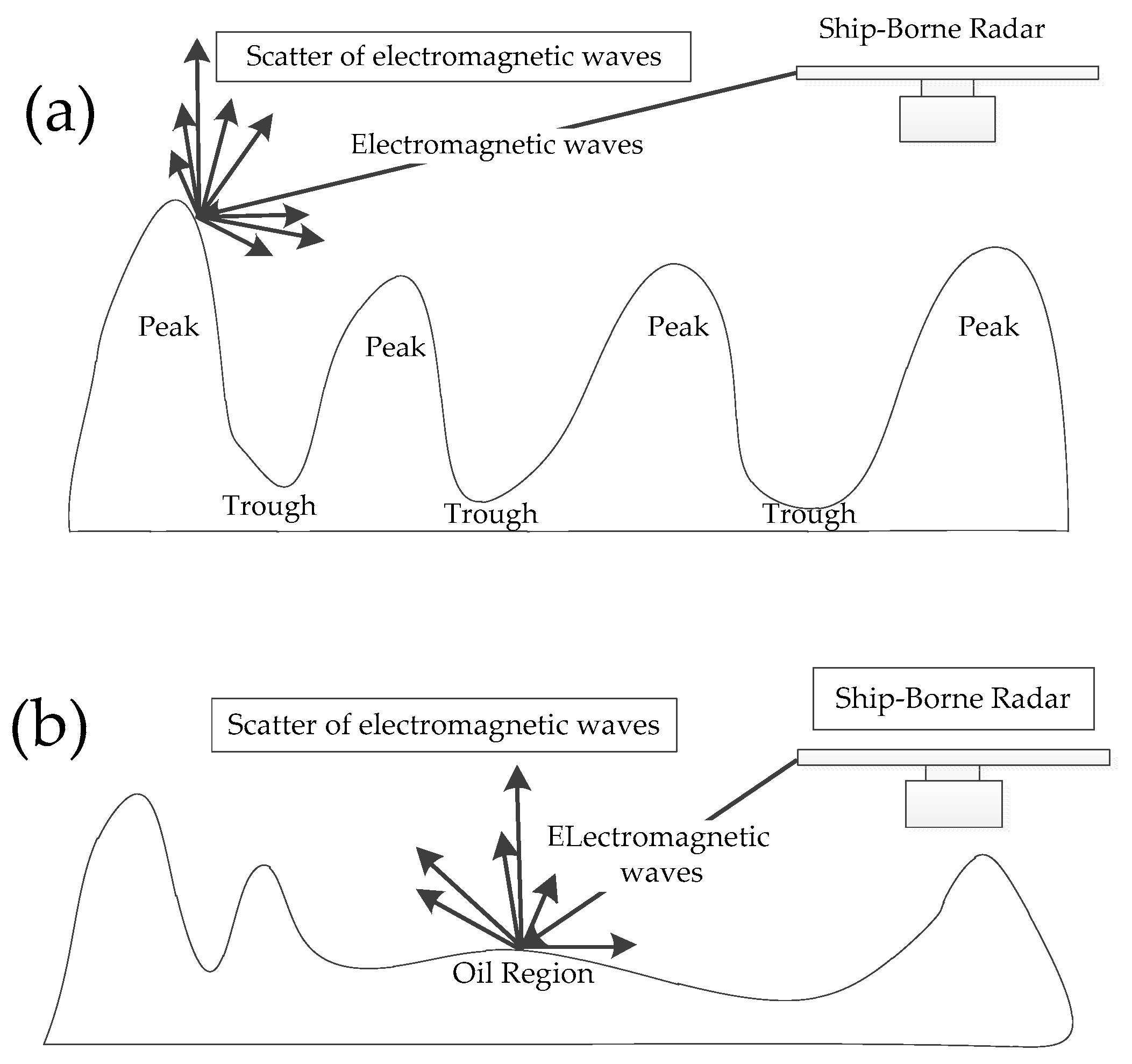
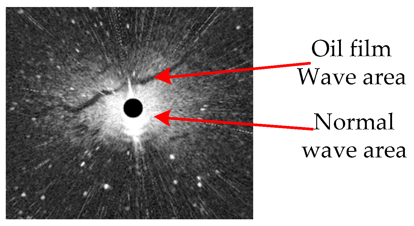
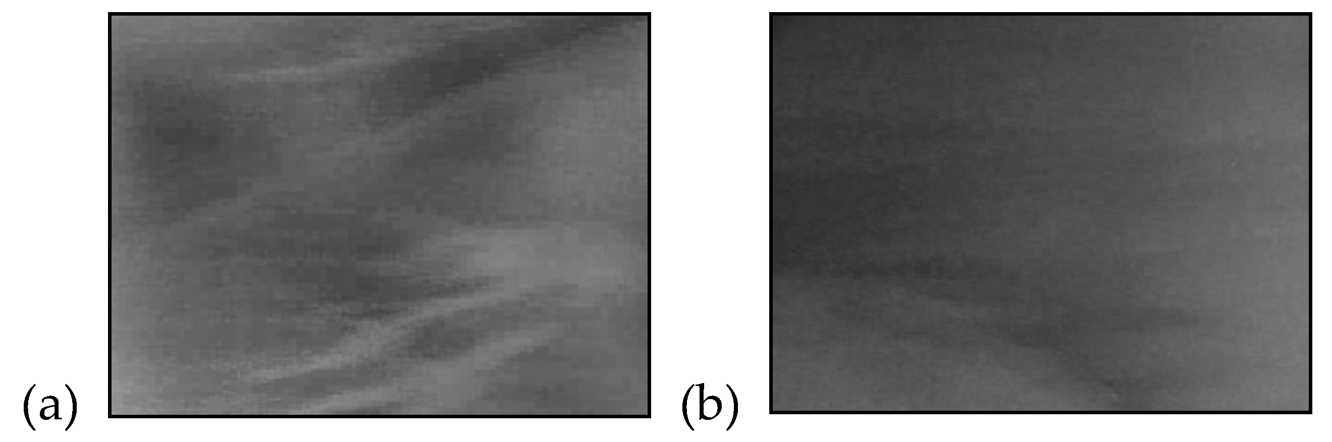
Ship-borne radar oil spill detection is based on the characteristics of sea clutter formed by Bragg scattering [42]. Sea waves are formed by integrated factors, such as gravitational waves, capillary waves, and wind force, which make the sea surface rough. Figure 1a shows a ship-borne radar transmitting electromagnetic waves onto the sea surface and receiving backscattered beams. However, the dampening effect of the oil spill on the cm-scale waves reduces the radar backscatter beams (Figure 1b), weakening the signal in the oil film region more than the area around it (Figure 2) [43]. It is worth mentioning that, when the sea surface is extremely calm, the wave echo grey intensity in a ship-borne radar image is too low for the detection of oil films. When the wind speed is very high, the oil undergoes mixing with seawater. This significantly reduces the ability of the oil film to suppress sea surface roughness, which makes it difficult to distinguish an oil spill from wave information in images in such conditions [42].
3. Classical ACMs
3.1. C-V Model
Chan and Vese [33] proposed a new active contour which represents an image as a piecewise constant function. A grey image I(x): Ω→R is divided into two regions, the target Rin and the background Rout, starting with a pre-set contour C represented by the following energy:
where Cin and Cout are constants that approximate the image intensities of Rin and Rout, respectively.
The two-term energies in (1) can be represented by a level set formulation, such that the energy minimization problem can be converted to solving a level set evolution equation. One major advantage of the CV model is its insensitivity to initialization. If the image intensities in either Rin or Rout are not homogeneous, Cin and Cout will not accurately fit the image intensities. As a result, the CV model cannot handle images with intensity inhomogeneities [36].
3.2. LBF Model
Li et al. [37] proposed a new region-based ACM with a variable level set formulation that is more applicable to grey intensity inhomogeneous images. The LBF energy is defined as:
where λ1 and λ2 are as previously defined. Differing from C1 and C2 in the CV model, f1(x) and f2(x) are spatially varying fitting functions. Furthermore, I(y) is the pixel intensity in a window around y, while K is a kernel function with the localization property the K(u) decreases and approaches zero as |u| increases. A Gaussian kernel was chosen as K(x) with a standard deviation of σ in the ACM:
Due to the localization property of K(u), the contribution of I(y) to the LBF energy decreases to zero as y moves away from the centre point x. This property helps the model to handle images with intensity inhomogeneities.
3.3. LGIF Model
The LGIF model combines the advantages of the CV and LBF models. The energy function of the LGIF model is:
where ϕ is the level set function, v and μ are positive constants, θ is a constant, and 0 ≤ θ ≤ 1. The parameter value θ should be very small for images with intensity inhomogeneities. P is a penalty function of its deviation from a signed distance:
and L is a length penalty term of the zero level set:
Finally, the Heaviside function H is approximated with a smooth function Hk:
where k is a positive constant.
The values of εLBF and εcv complement each other in the contour evolution. When the contour is near object boundaries, εLBF is dominant. When the contour is far away from the boundaries, εcv is dominant while εLBF is close to zero [38]. The LGIF model further improves the global segmentation effects that occur with objects in images containing intensity inhomogeneities.
3.4. LIF Model
The LIF model formulation is defined as:
where m1 and m2 are:
and Wk(x) is a rectangular window function, such as a truncated Gaussian or constant window. A truncated Gaussian window Kσ(x) with standard deviation σ and size 4k + 1 by 4k + 1 was chosen, where k is the greatest integer smaller than σ.
Zhang et al. [41] proposed a LIF energy function that minimizes the difference between the fitted image and the original image:
εLIF was minimized by the calculus of variations and the steepest descent method:
where δε is the regularized Dirac function is defined as
4. Materials and Methods
4.1. Data
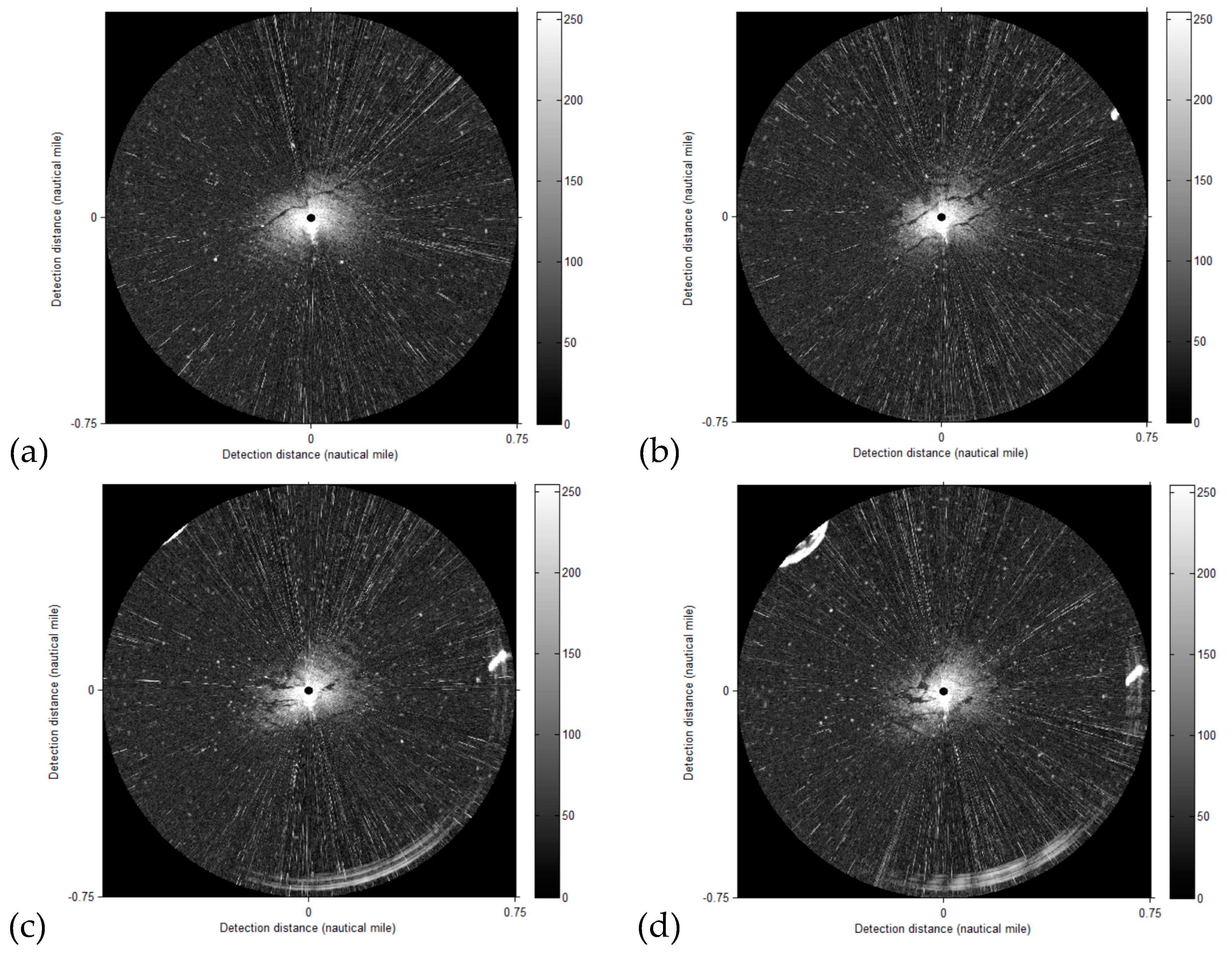
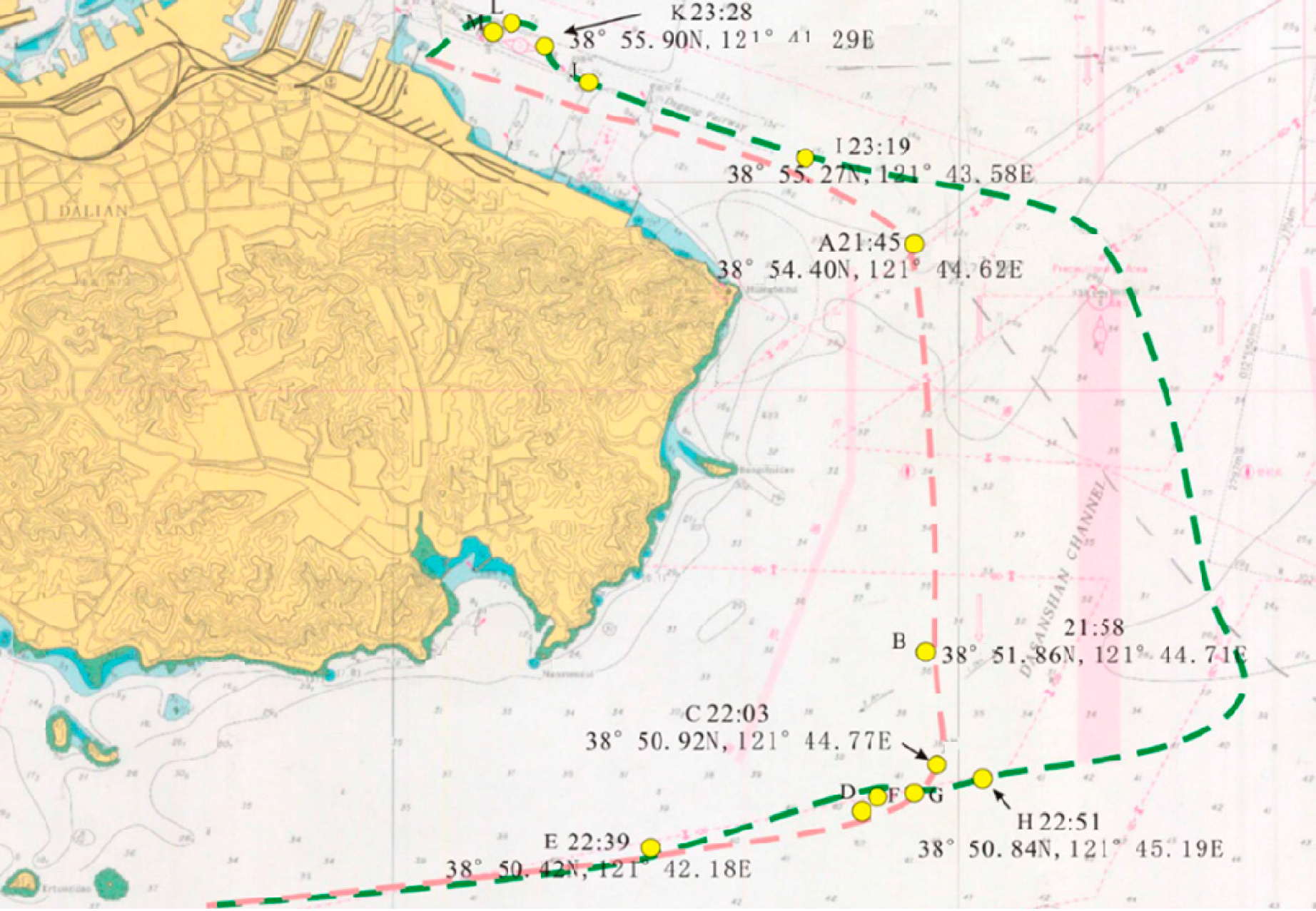
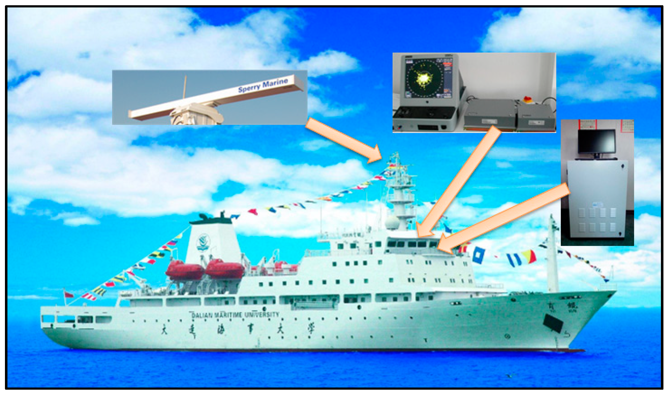
The experimental data were 68 primary radar images (Figure 3) containing oil films, acquired during the clean-up mission (Figure 4) on 21 July 2010 after the Dalian “7-16” oil spill accident. The data acquisition radius was 0.75 nautical miles (NM), the image size was 1024 × 1024, and the data acquisition cycle was 2 seconds. The platform of the ship-borne radar was the teach-training ship Yukun of Dalian Maritime University (Figure 5). The data acquisition card was SPx-200 of Sperry Marine B.V. Radar. Parameters are listed in Table 1.
4.2. Image Pre-Processing
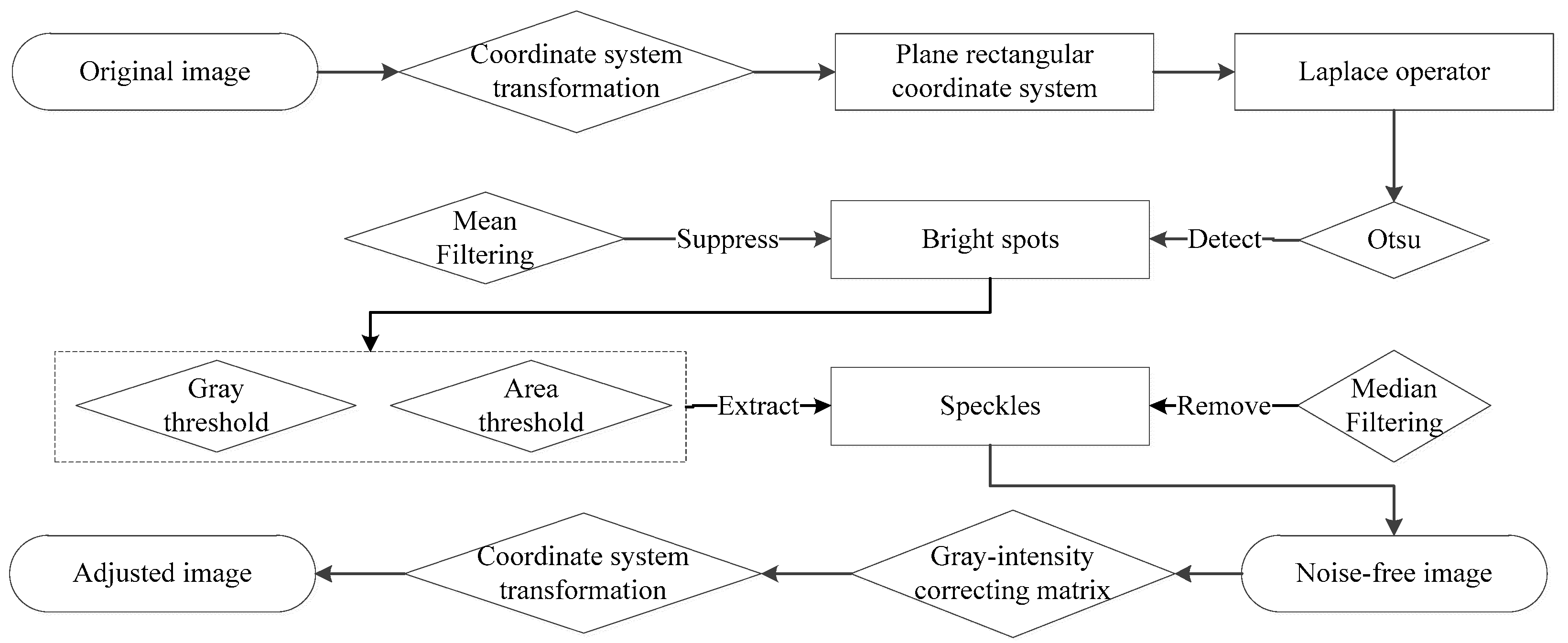
Original images captured from ship-borne radar always contain co-channel interference, bright spots, and speckles. It was, therefore, necessary to smooth the noise, in order to reduce inhomogeneities. A ship-borne radar image is transformed into a polar co-ordinate system after being generated in a plane rectangular co-ordinate system. Therefore, we suggested restoring the image to the plane rectangular co-ordinate system for pre-processing. A Laplace operator was used to enhance co-channel interference and pixel brightness, while the Otsu threshold method [46] was selected to extract pixels to be processed. Subsequently, the grey values of adjacent non-noisy pixels were used for smoothing. Grey and area thresholds were used to extract speckles, which were removed by the median filter. Next, GICM was used to correct the radar image. A pre-processing flow diagram is shown in Figure 6.
4.2.1. Smoothing of Co-Channel Interference and Bright Spots
A Laplace operator is a second-order differential operator in n-D Euclidean space. For a 2D function f(x, y), a Laplace operator is expressed as:
where its window filter is:
A different form of the Laplace operator is used here to highlight the pixels to be processed:
where its window filter is:
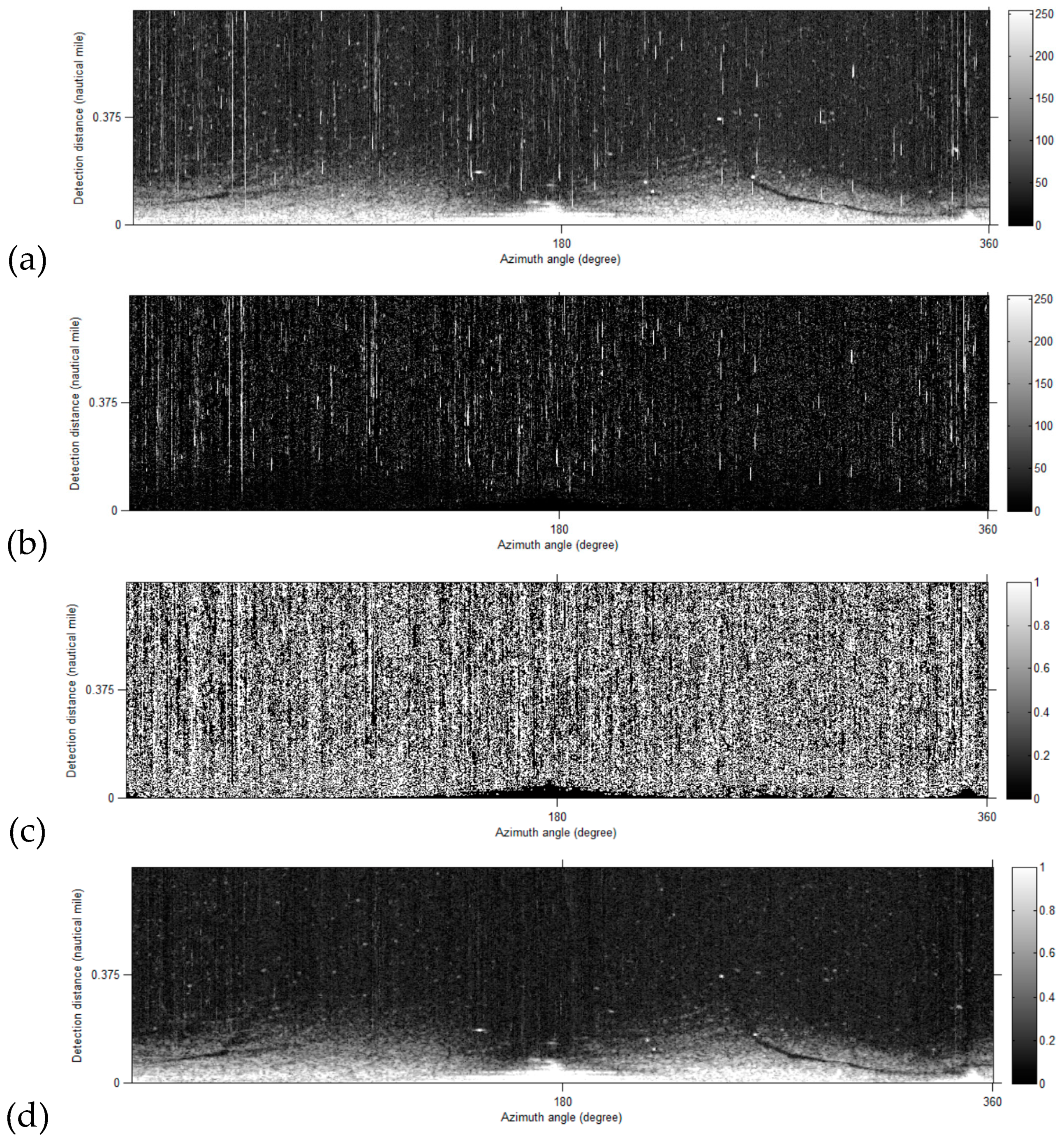
After the noises were segmented by the Otsu threshold, mean filtering was used to remove them (Figure 7). Two adjacent non-noisy points along the x-axis in the plane rectangular co-ordinate system are computed as:
where m and n are the distances between the nearest non-noisy points on the left and right, respectively.
4.2.2. Suppression of Other Noise
Speckles or objects other than waves were considered as noise, defined by:
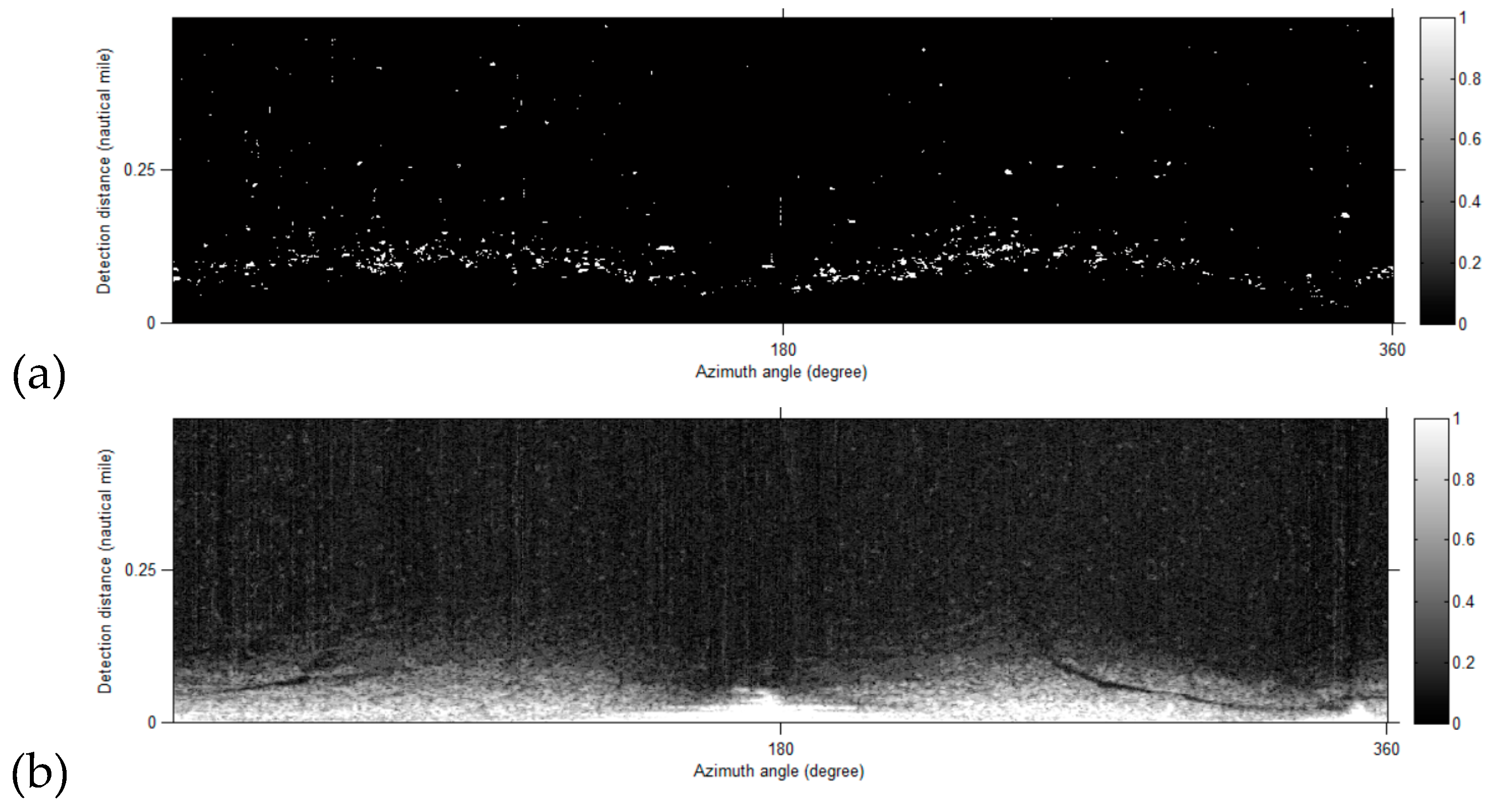
where Tgrey is the grey threshold, Count(x) is the number of continuous pixels with a grey value greater than Tgrey, and Tarea is the numeric threshold of continuous pixels. Median filtering with a window greater than twice Tarea was used to suppress N(x), as shown in Figure 8.
4.2.3. Image Rectification
The electromagnetic wave echo decreased with increasing distance in the original images. Thus, the GICM (Figure 9) was proposed to rectify the images (Figure 10). The column vector C1 was obtained by averaging the rows of sample M1. The rows of M2 were then filled with the values given in the rows of C1. Thus, the image was transformed to a polar co-ordinate system (Figure 11).
4.3. Proposed Method
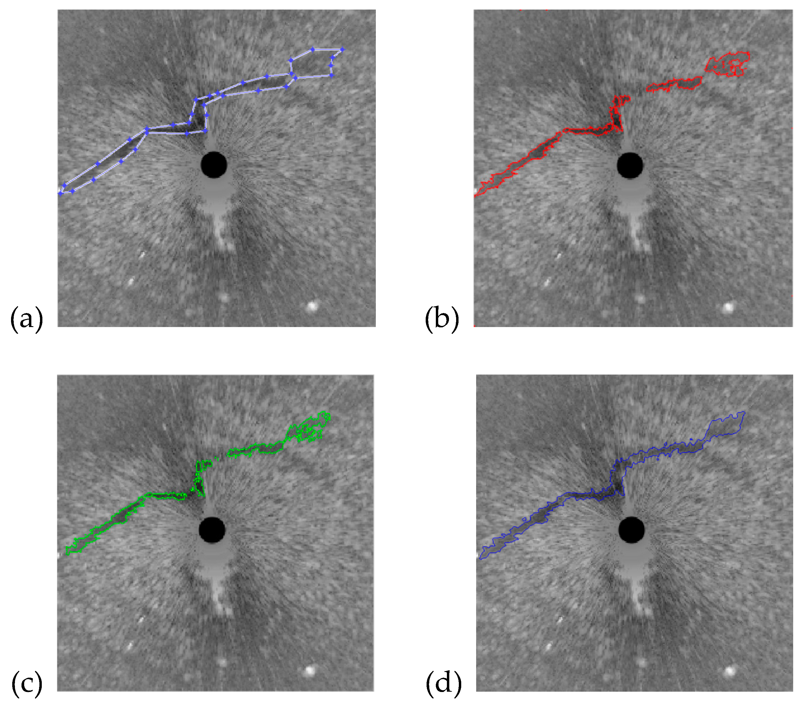
A ship-borne radar image (Figure 12a) containing islands is used to explain our proposed improved active contour model. As the intensity of a ship-borne radar is very inhomogeneous, ACM recognition results have small error targets, as shown in Figure 12. We call the number of pixels of a target (non-discrete region) in the image a continuous pixel area. In order to remove false positive targets and speckles to optimize the preliminary recognition results, we propose a continuous pixel area threshold parameter D(x) to improve ACMs:
where rin and rout belong to the regions inside and outside the counter, respectively; A is the area of continuous pixels; and Tin and Tout are the area thresholds of rin and rout, respectively. The implementation of the process is shown in Figure 13.
As the range and size of the image are known, the actual area A(x) of each pixel can be obtained, meaning that the area Aresult of the target can be calculated by:
Setting Tout and Tin is key; if Tin was set to ‘30′, the suspected small oil film of 220.8 m2 would be removed from the 1024 × 1024 ship-borne radar images, with a range of 0.75 NM.
5. Results and Discussion
5.1. Results
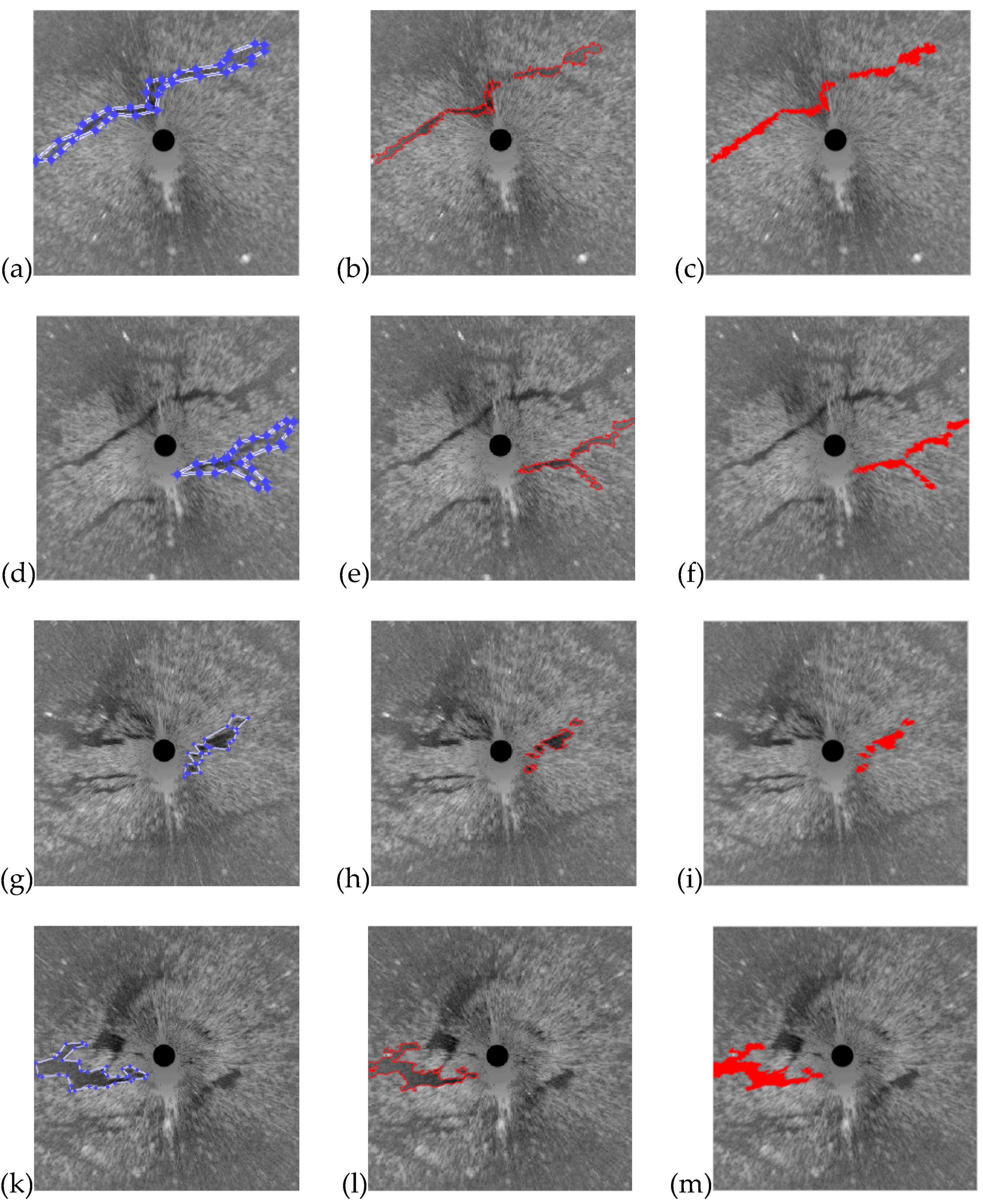
The image pre-processing methods of Section 4.2 were used to deal with the experimental images, as shown in Figure 12. The pre-processed data were analysed by both the original and improved LBF models, as shown in Figure 14, where i = 10, λ1 = 1, λ2 = 2, σ = 3, Tin = 20, and Tout = 20. According to the range and size of the data, the identified oil film area could be computed, as shown in Table 2. After pre-processing, the original oil film profile could be obtained by directly using LBF model, but contained speckles, as can be seen in Figure 15b,e,h,l. The proposed method could obtain a more accurate oil film area, as shown in Figure 15c,f,i,m.
5.2. Verification
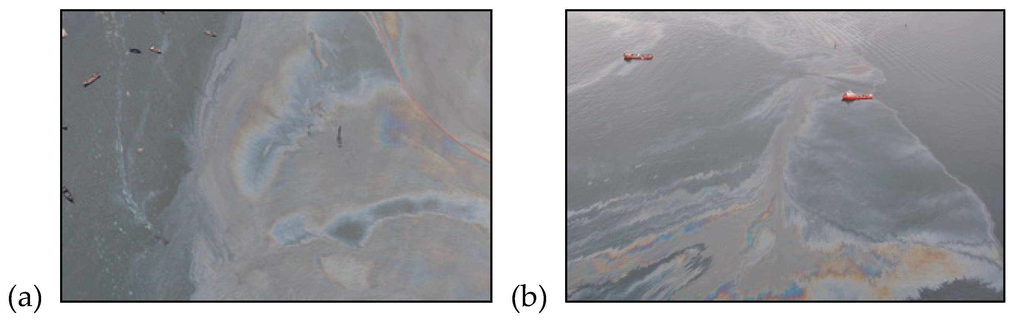
In practice, there are many look-alikes similar to oil spills, such as biogenic films, low-wind areas, or rain cells, which can generate relatively dark areas in ship-borne radar images. In daytime cases, the distinction between oil spills and look-alikes is based on visible light or optical data [42]. In visible light images obtained from an airborne camera (Figure 16), many oil films can be monitored during daytime hours. However, the experimental data were acquired at night. The verification data (Figure 17) were derived from the ship-borne thermal infrared detector. At night, oil films have somewhat lower grey values than water in thermal infrared images [42]. Oil film information can also be extracted from thermal infrared images captured around the ship where oil slicks were found in ship-borne radar images.
5.3. Limitations of Ship-Borne Radar Oil Spill Monitoring Technology
Compared to satellite-borne and airborne techniques, ship-borne remote sensors can be easily operated, have high resolution, and are not affected by poor weather conditions, making them very effective in monitoring oil spill emergencies. Other advantages of ship-borne radar include its ability to monitor oil spills over large distances, wide range, and low modification costs. However, despite its promise, there are still some limitations to the use of ship-borne radar oil spill monitoring technology.
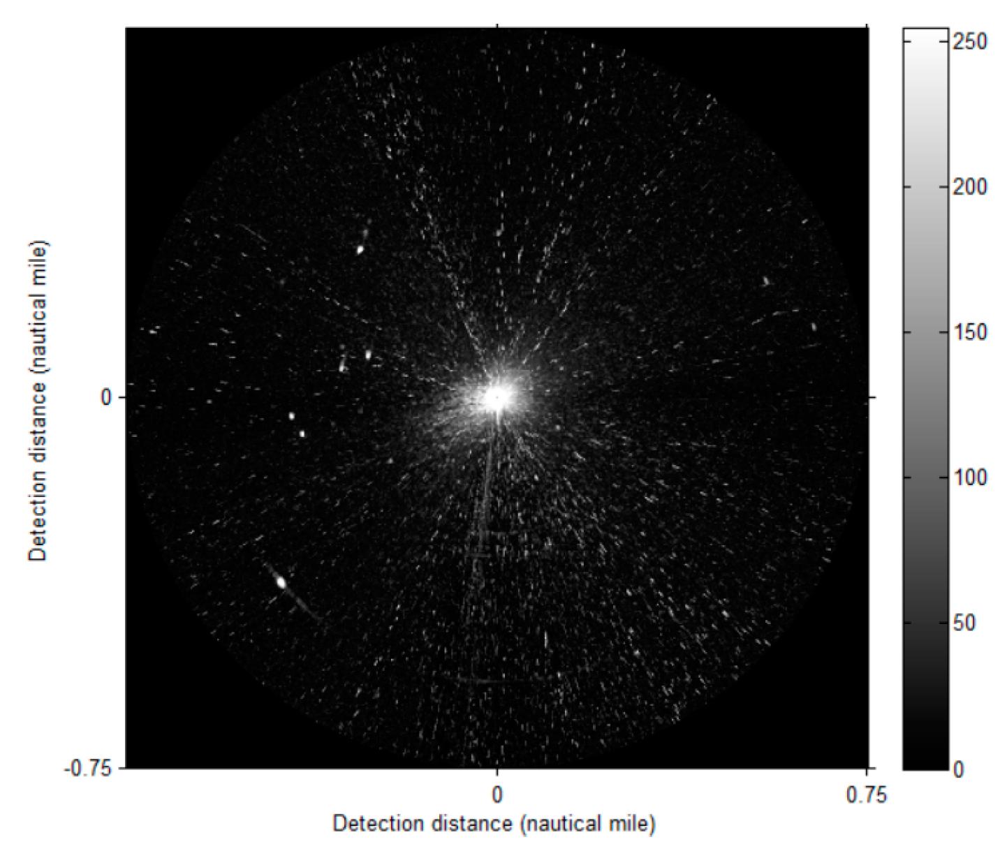
First, ship-borne radar monitoring technology is highly dependent on sea conditions. When waves are too strong, the ship cannot launch out to clean up the pollution. When the sea surface is too calm, the radar cannot retrieve a wide range of wave echoes, as shown in Figure 18; then, it is difficult to recognize oil films in such a sea clutter image.
Second, image resolution directly affects result accuracy. In the experimental data, the actual area represented by each pixel was 7.36 m2. If a pixel is identified as oil film, the entire 7.36 m2 sea surface is identified as covered by oil film. Improving recognition accuracy requires upgrading the remote sensing sensors, as well as further breakthroughs in image generation technology.
5.4. Comparison with Other ACMS
The LBF, LGIF, and LIF models were applied to Figure 15a and shown in Figure 19. To do this, we set i = 5, λ1 = 1, λ2 = 2, and σ = 2; the contrasting terms are shown in Table 3. The LBF and LGIF models only fit the oil films near the initial contour, but the LIF model continuously calculated outward. Although the LIF model had the fastest speed and largest segmentation area, it was not effective in target recognition outside the initial contour. In addition, the LBF model conformed better to the visual interpretation results than the LGIF model did. Furthermore, the LBF model exhibited a faster calculation speed than the LGIF model. Therefore, the LBF model is more suitable as a basic ACM for ship-borne radar image segmentation.
5.5. Parameter Choices
After increasing i with the pre-set contour of Figure 15k, the segmentation effect was not improved, as shown in Figure 20a–c. This indicates that, as i rises, to a certain extent, the evolution of the level set is not obvious, with only a slight adjustment. Furthermore, the LBF model limits the target contour evolution to a small local area, according to the pre-set contour. A larger scale parameter σ of the Gaussian kernel would make the LBF model more robust to an inhomogeneous image [36]. By setting σ = 3, as in Figure 20d–f, the effect of contour recognition greatly improved. However, enlarging σ will increase the calculation time, as shown in Table 4. Therefore, we recommend setting σ = 3 for oil film detection.
After adjusting the value of λ2 to 1, as in Figure 20g–i, the level set evolved dramatically. After identifying the target near the initial contour, the LBF model could quickly compute outward. This indicates that λ2 was a major parameter constraining the contour evolution region. We suggest setting λ1 = 1, λ2 = 2, σ = 3, and i = 10.
5.6. Applicability of Whole Oil Films
In Figure 15c, our method achieved good recognition results for strip discrete oil films. The next experiment is to handle irregular discrete oil films. By setting λ1 = 1, λ2 = 1, σ = 5, and i = 10, the three ACMs could achieve the global segmentation results shown in Figure 21. As the corrected image was still very uneven, the ACMs created many wrong segmentation results after global segmentation. The LBF model had a better segmentation effect, but also a large number of suspected targets. Therefore, perfect smoothing remains a large challenge prior to oil film analysis of the whole image.
5.7. Comparison with Other Methods
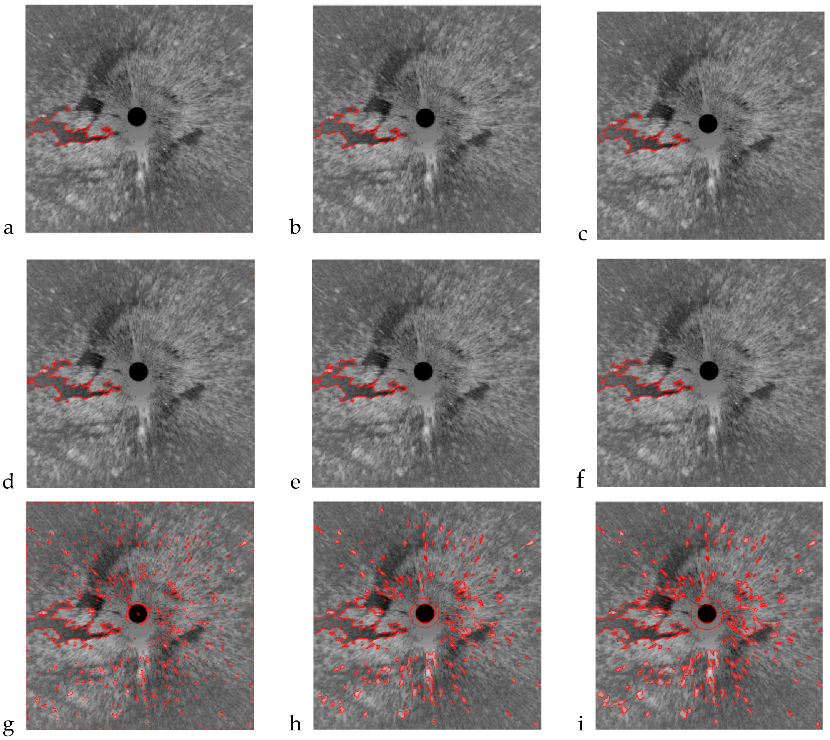
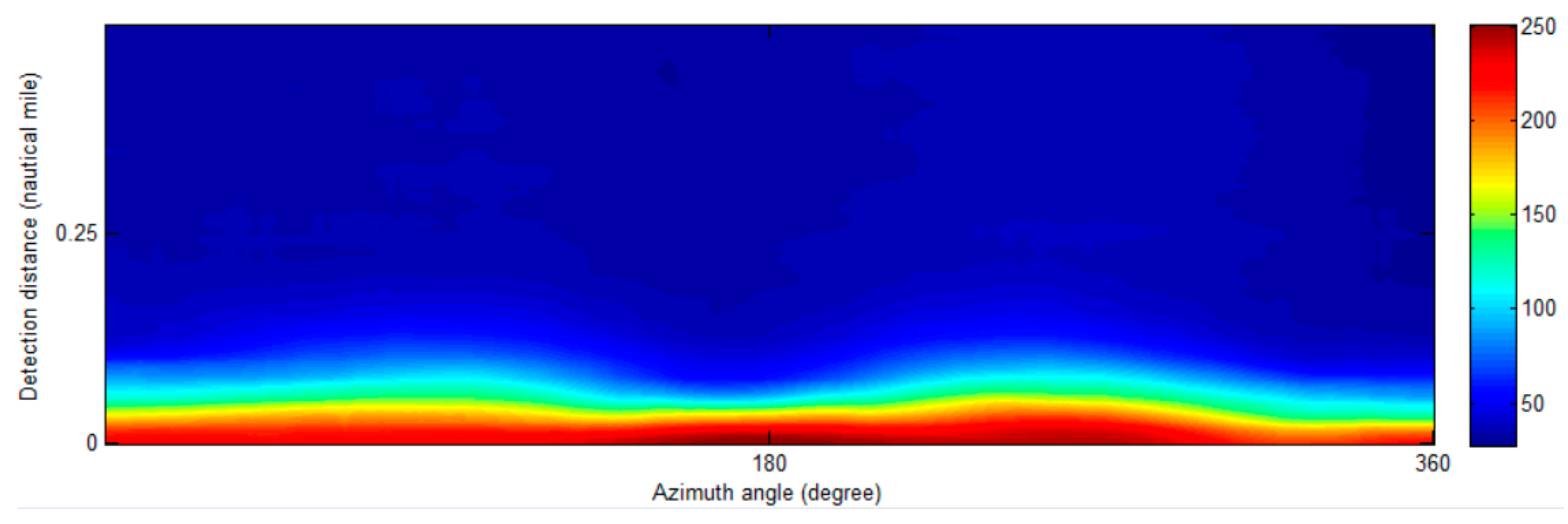
Zhu et al. [24], Liu et al. [25], and Xu et al. [26] proposed different identification methods for oil films in ship-borne radar images. We compared our method with their approaches in Figure 22. After adjustment, the grey threshold of Figure 22a was 110. After choosing the appropriate threshold to intercept the effective wave area in Figure 23 (the segment values were 58 and 100 for Figure 22b,c, respectively), Liu’s [23] method uses a local window and Otsu threshold to detect oil films (Figure 22b). Xu’s method [24] uses a grey threshold of 100 and area threshold of 250 (Figure 22c). The parameters of our method were λ1 = 1, λ2 = 2, σ = 3, and i = 10. A comparison of the computation time and pixel area is shown in Table 5.
Figure 22a–c applied the global segmentation method, causing some erroneous results. Our method started with an initial contour around the oil films, in order to lock the approximate segmentation region. The results are more in line with the visual interpretation. Through pre-processing, the co-ordinate system transformation was realized and the final colour image synthesis took less time using our method. In other methods, the oil films were distinguished in Cartesian co-ordinates, and the co-ordinate system was transformed after the colour image was synthesized. Furthermore, the methods of Liu [25] and Xu [26] created a decision matrix for the effective wave area, which took more time. Therefore, our method is more efficient for data analysis.
6. Conclusions
In this paper, we propose a pre-processing method to eliminate co-channel interference and speckles in original ship-borne radar images. It can provide a good pre-processing scheme for wave information inversion from ship-borne radar images. An improved LBF model using a pixel area threshold parameter is proposed for oil film detection. Compared to other ACMs, the improved LBF model is robust and exhibits a fast calculation speed for uniform ship-borne radar images. Our method can extract the distribution range and the area of an oil film and provide a technical basis for emergency clean-up and damage assessment of oil spill accidents. In addition, our method can provide data samples for deep learning methods for oil film recognition in ship-borne radar images.
Author Contributions
J.X. conceived, design and performed the experiments; H.W. and C.C. collected data and helped perform the analysis with constructive discussions and revised the manuscript; P.L., Y.Z. and B.L. contributed to revisions and approved the final version.
Acknowledgments
This research was funded by the National Natural Science Foundation of China [grant number 51709031], the Fundamental Research Funds for the Central Universities [grant number 3132019138] and the Innovation Support Project of Dalian [grant number 2018RQ22].
Conflicts of Interest
The authors declare no conflict of interest.
References
- Migliaccio, M.; Gambardella, A.; Tranfaglia, M. SAR Polarimetry to Observe Oil Spills. IEEE Trans. Geosci. Remote Sens. 2007, 45, 506–511. [Google Scholar] [CrossRef]
- Nunziata, F.; Macedo de, C.R.; Buono, A.; Velotto, D.; Migliaccio, M. On the analysis of a time series of X–band TerraSAR–X SAR imagery over oil seepages. Int. J. Remote Sens. 2019, 40, 3623–3646. [Google Scholar] [CrossRef]
- Yang, J.; Jin, S.; Xiao, X.; Jin, C.; Xia, C.; Lia, X.; Wang, S. Local Climate Zone Ventilation and Urban Land Surface Temperatures: Towards a Performance-based and Wind-sensitive Planning Proposal in Megacities. Sustain. Cities Soc. 2019, 47, 1–11. [Google Scholar] [CrossRef]
- Yang, J.; Wang, C.; Xiao, X.; Jin, C.; Xia, J.; Li, X. Spatial differentiation of urban wind and thermal environment in different grid sizes. Urban Clim. 2019, 28, 100458. [Google Scholar] [CrossRef]
- Tzannatos, E.; Xirouchakis, A. Techno-economic assessment of hull-mounted sonar for oil-spill risk Control. J. Navig. 2013, 66, 625–636. [Google Scholar] [CrossRef]
- Hsu, W.; Lian, S.; Huang, S. Risk assessment of operational safety for oil tankers—A revised risk matrix. J. Navig. 2017, 70, 775–788. [Google Scholar] [CrossRef]
- Gambardella, A.; Giacinto, G.; Migliaccio, M.; Montali, A. One-class classification for oil spill detection. Pattern Anal. Appl. 2010, 13, 349–366. [Google Scholar] [CrossRef]
- Yang, J.; Guan, Y.; Xia, J.; Jin, C.; Li, X. Spatiotemporal variations in greenspace ecosystem service value at urban fringes: A case study on Ganjingzi District in Dalian, China. Sci. Total Environ. 2018, 639, 1453–1461. [Google Scholar] [CrossRef]
- Carvalho, G.; Minnett, P.; Miranda, F.D.; Landau, L.; Paes, E. Exploratory data analysis of Synthetic Aperture Radar (SAR) measurements to distinguish the sea surface expressions of naturally-occurring oil seeps from human-related oil spills in Campeche Bay (Gulf of Mexico). Int. J. Geo Inf. 2017, 6, 379. [Google Scholar] [CrossRef]
- Cao, Y.; Xu, L.; Clausi, D. Exploring the potential of active learning for automatic identification of marine oil spills using 10-Year (2004–2013) RADASAT data. Remote Sens. 2017, 9, 1041. [Google Scholar] [CrossRef]
- Chen, G.; Li, Y.; Sun, G.; Zhang, Y. Application of deep networks to oil spill detection using polarimetric Synthetic Aperture Radar images. Appl. Sci. 2017, 7, 968. [Google Scholar] [CrossRef]
- Guo, H.; Wu, D.; An, J. Discrimination of oil slicks and lookalikes in polarimetric SAR images using CNN. Sensors 2017, 17, 1837. [Google Scholar] [CrossRef] [PubMed]
- Song, D.; Ding, Y.; Li, X.; Zhang, B.; Xu, M. Ocean oil spill classification with RADARSAT-2 SAR based on an Optimized Wavelet Neural Network. Remote Sens. 2017, 9, 799. [Google Scholar] [CrossRef]
- Lupidi, A.; Staglianò, D.; Martorella, M.; Berizzi, F. Fast detection of oil spills and ships using SAR images. Remote Sens. 2017, 9, 230. [Google Scholar] [CrossRef]
- Angelliaume, S.; Ceamanos, X.; Viallefontrobinet, F.; Baqué, R.; Déliot, P. Hyperspectral and radar airborne imagery over controlled release of oil at sea. Sensors 2017, 17, 428. [Google Scholar] [CrossRef] [PubMed]
- Jones, C.E.; Holt, B. Experimental L-band airborne SAR for oil spill response at sea and in coastal waters. Sensors 2018, 18, 641. [Google Scholar] [CrossRef]
- Gallego, A.J.; Gil, P.; Pertusa, A.; Fisher, R.B. Segmentation of oil spills on side-looking airborne radar imagery with autoencoders. Sensors 2018, 18, 797. [Google Scholar] [CrossRef]
- Tennyson, E.J. Shipboard navigational radar as an oil spill tracking tool-a preliminary assessment. In Proceedings of the OCEANS 1988, Baltimore, MD, USA, 31 October–2 November 1988; pp. 857–859. [Google Scholar] [CrossRef]
- Atanassov, V.; Mladenov, L.; Rangelov, R.; Savchenko, A. Observation of oil slicks on the sea surface by using marine navigation radar. In Proceedings of the IGARSS 1991, Espoo, Finland, 3–6 June 1991; pp. 1323–1326. [Google Scholar] [CrossRef]
- Gangeskar, R. Automatic oil-spill detection by marine X-band radars. Sea Technol. 2004, 45, 40–45. [Google Scholar] [CrossRef]
- Chu, X.L.; Ming, X.U.; Wang, F.; Wang, J. Analysis of the wave information extracted by X-band radar. Period. Ocean Univ. China 2011, 41, 110–113. [Google Scholar]
- Nost, E.; Egset, C.N. Oil spill detection system—Results from field trials. In Proceedings of the OCEANS 2006, Boston, MA, USA, 18–21 September 2006. [Google Scholar] [CrossRef]
- Egset, C.N.; Nost, E. Oil spill detection system based on marine X-band radar. Sea Technol. 2007, 48, 41–45. [Google Scholar]
- Zhu, X.; Li, Y.; Feng, H.; Liu, B.; Xu, J. Oil spill detection method using X-band marine radar imagery. J. Appl. Remote Sens. 2015, 9, 095985. [Google Scholar] [CrossRef]
- Liu, P.; Li, Y.; Xu, J.; Zhu, X. Adaptive enhancement of X-band marine radar imagery to detect oil spill segments. Sensors 2017, 17, 2349. [Google Scholar] [CrossRef]
- Xu, J.; Liu, P.; Wang, H.; Lian, J.; Li, B. Marine radar oil spill monitoring technology based on Dual-threshold and C–V level set methods. Indian Soc. Remote Sens. 2018, 46, 1949–1961. [Google Scholar] [CrossRef]
- Xu, J.; Cui, C.; Feng, H.Y.; You, D.M.; Wang, H.X.; Li, B. Marine Radar Oil-Spill Monitoring through Local Adaptive Thresholding. Environ. Forensics 2019, 20, 196–209. [Google Scholar] [CrossRef]
- Zhang, X.; Xiong, B.; Dong, G.; Kuang, G. Ship segmentation in SAR images by improved nonlocal active contour model. Sensors 2018, 18, 4220. [Google Scholar] [CrossRef] [PubMed]
- Liu, J.; Wen, X.; Meng, Q.; Xu, H.; Yuan, L. Synthetic aperture radar image segmentation with reaction diffusion level set evolution equation in an active contour model. Remote Sens. 2018, 10, 906. [Google Scholar] [CrossRef]
- Kass, M.; Witkin, A.; Terzopoulos, D. Snakes: Active contour models. Int. J. Comput. Vis. 1988, 1, 321–331. [Google Scholar] [CrossRef]
- Xu, C.; Prince, J.L. Snakes, shapes, and gradient vector flow. IEEE Trans. Image Process. 1998, 7, 359–369. [Google Scholar] [CrossRef]
- Xu, C.; Prince, J.L. Generalized gradient vector flow external forces for active contours. Signal Process. 1998, 71, 131–139. [Google Scholar] [CrossRef] [Green Version]
- Caselles, V.; Kimmel, R.; Sapiro, G. Geodesic active contours. Int. J. Comput. Vis. 1997, 22, 61–79. [Google Scholar] [CrossRef]
- Chan, T.F.; Vese, L.A. Active contours without edges. IEEE Trans. Image Process. 2001, 10, 266–277. [Google Scholar] [CrossRef] [PubMed] [Green Version]
- Mumford, D.; Shah, J. Optimal approximation by piecewise smooth function and associated variational problems. Commun. Pure Appl. Math. 1989, 42, 577–685. [Google Scholar] [CrossRef]
- Vese, L.A.; Chan, T.F. A multiphase level set framework for image segmentation using the Mumford and Shah model. Int. J. Comput. Vis. 2002, 50, 271–293. [Google Scholar] [CrossRef]
- Li, C.M.; Kao, C.Y.; Gore, J.C.; Ding, Z. Minimization of regionscalable fitting energy for image segmentation. IEEE Trans. Image Process. 2008, 17, 1940–1949. [Google Scholar] [CrossRef] [PubMed]
- Wang, L.; Li, C.; Sun, Q.; Xia, D.; Kao, C. Active contours driven by local and global intensity fitting energy with application to brain MR image segmentation. Comput. Med. Imaging Graph. 2009, 33, 520–531. [Google Scholar] [CrossRef]
- Wang, L.; He, L.; Mishra, A.; Li, C. Active contours driven by local Gaussian distribution fitting energy. Signal Process 2009, 89, 2435–2447. [Google Scholar] [CrossRef]
- Thieu, Q.; Luong, M.; Rocchisani, J.; Sirakov, N.M.; Viennet, E. Efficient segmentation with the convex local-global fuzzy Gaussian distribution active contour for medical applications. Ann. Math. Artif. Intell. 2015, 75, 249–266. [Google Scholar] [CrossRef]
- Zhang, K.H.; Song, H.H.; Zhang, L. Active contours driven by local image fitting energy. Pattern Recognit. 2010, 43, 1199–1206. [Google Scholar] [CrossRef]
- Fingas, M.; Brown, C.E. A review of oil spill remote sensing. Sensors 2018, 18, 91. [Google Scholar] [CrossRef]
- Brekke, C.; Solberg, A.H.S. Oil spill detection by satellite remote sensing. Remote Sens. Environ. 2005, 95, 1–13. [Google Scholar] [CrossRef]
- Ji, Z.X.; Xia, Y.; Sun, Q.S.; Gao, G.; Chen, Q. Active contours driven by local likelihood image fitting energy for image segmentation. Inf. Sci. 2015, 301, 285–304. [Google Scholar] [CrossRef]
- Sun, L.; Meng, X.; Xu, J.; Tian, Y. An Image Segmentation Method Using an Active Contour Model Based on Improved SPF and LIF. Appl. Sci. 2018, 8, 2576. [Google Scholar] [CrossRef]
- Otsu, N. A threshold selection method from gray-level histograms. IEEE Trans. Syst. Man Cybern. 1979, 9, 62–66. [Google Scholar] [CrossRef]
Figure 1.
Ship-borne radar oil spill detection mechanism. Radar electromagnetic wave echo-creation principles are shown for (a) a normal sea surface and (b) an oil-film area.
Figure 1.
Ship-borne radar oil spill detection mechanism. Radar electromagnetic wave echo-creation principles are shown for (a) a normal sea surface and (b) an oil-film area.

Figure 2.
Comparison between normal and oil film wave regions.

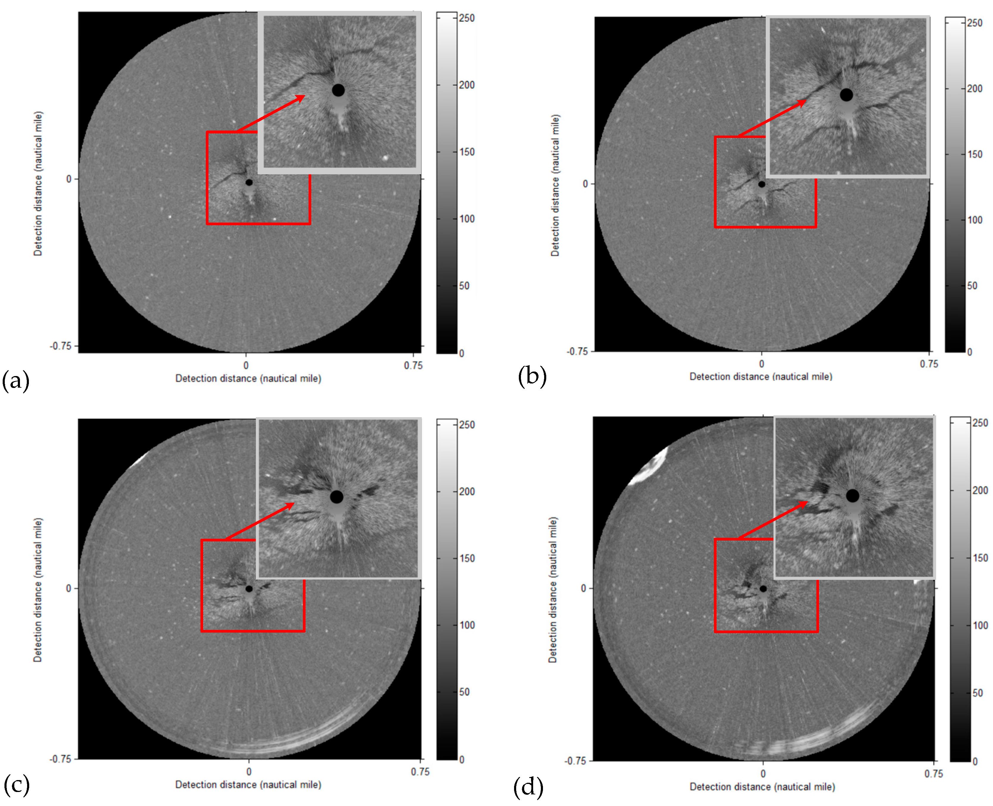
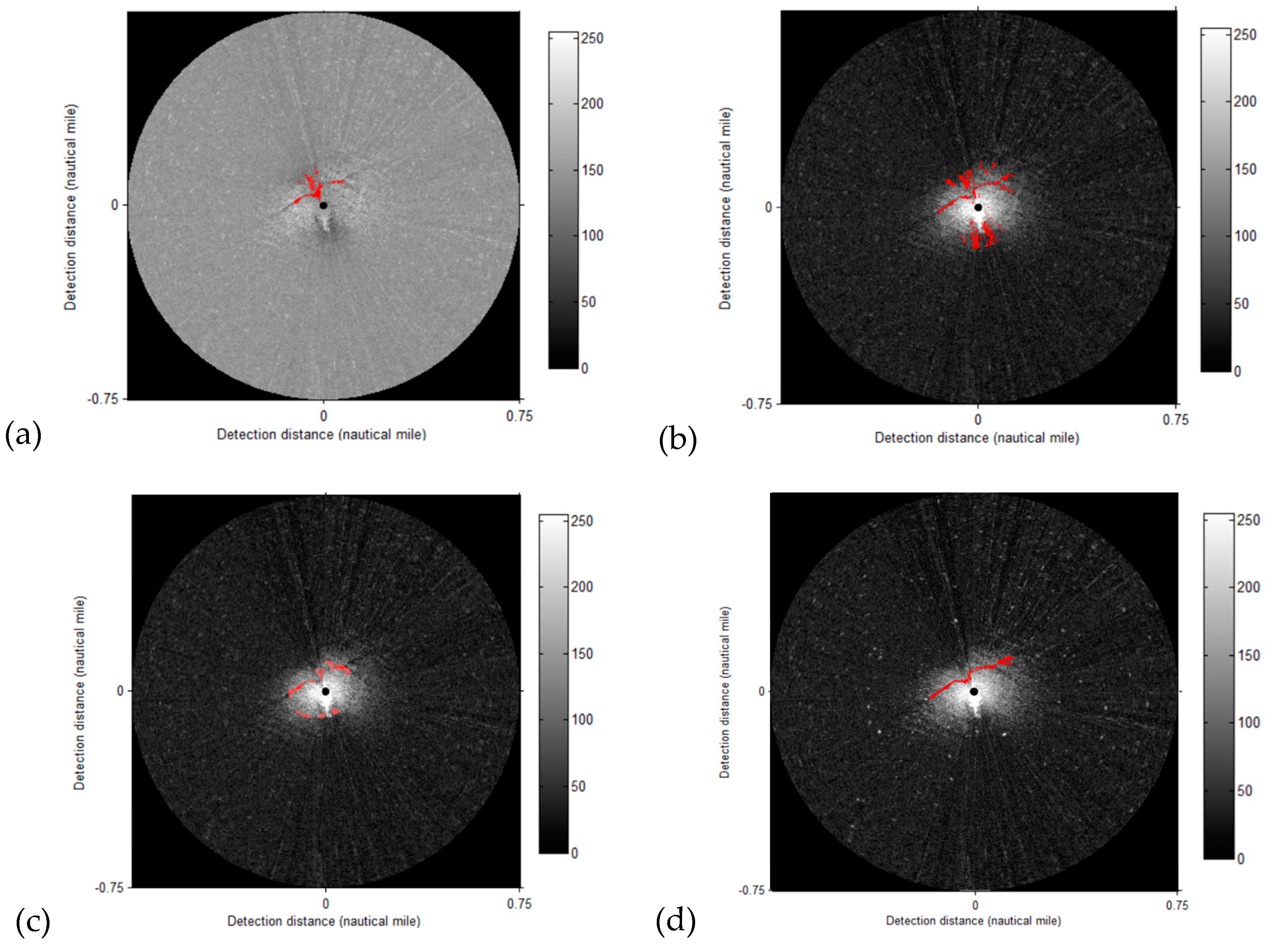
Figure 3.
Primary experimental images of 68 oil spill radar images during the cleanup of the Dalian “7-16” oil spill accident. (a–d) were collected at 23:19:11, 23:19:43, 23:20:57, and 23:21:09, respectively.
Figure 3.
Primary experimental images of 68 oil spill radar images during the cleanup of the Dalian “7-16” oil spill accident. (a–d) were collected at 23:19:11, 23:19:43, 23:20:57, and 23:21:09, respectively.

Figure 4.
Overview of the oil spill cleanup mission. The red and green lines are the departure and return routes, respectively.
Figure 4.
Overview of the oil spill cleanup mission. The red and green lines are the departure and return routes, respectively.

Figure 5.
Installation of the ship-borne radar oil spill data acquisition system onboard the Yukun [26].
Figure 5.
Installation of the ship-borne radar oil spill data acquisition system onboard the Yukun [26].

Figure 6.
Flow diagram for image pre-processing.

Figure 7.
Smoothing of Figure 3a. (a) The original image in a plane rectangular co-ordinate system; (b) convolution with a Laplace operator; (c) application of the Otsu method; (d) smoothing result.
Figure 7.
Smoothing of Figure 3a. (a) The original image in a plane rectangular co-ordinate system; (b) convolution with a Laplace operator; (c) application of the Otsu method; (d) smoothing result.

Figure 8.
Noise reduction of Figure 7d: (a) Noise extraction; and (b) median filtering. Tgrey = 100, Tarea = 200, and the median filtering window is 21 × 21.
Figure 8.
Noise reduction of Figure 7d: (a) Noise extraction; and (b) median filtering. Tgrey = 100, Tarea = 200, and the median filtering window is 21 × 21.

Figure 9.
Diagram of the Grey Intensity Correcting Matrix (GICM) model. Every grey value is calculated using the mean value of each respective row.
Figure 9.
Diagram of the Grey Intensity Correcting Matrix (GICM) model. Every grey value is calculated using the mean value of each respective row.

Figure 10.
Image rectification of Figure 8b. (a) GICM; and (b) rectification result.
Figure 10.
Image rectification of Figure 8b. (a) GICM; and (b) rectification result.

Figure 11.
Data pre-processing result of Figure 3a.
Figure 11.
Data pre-processing result of Figure 3a.

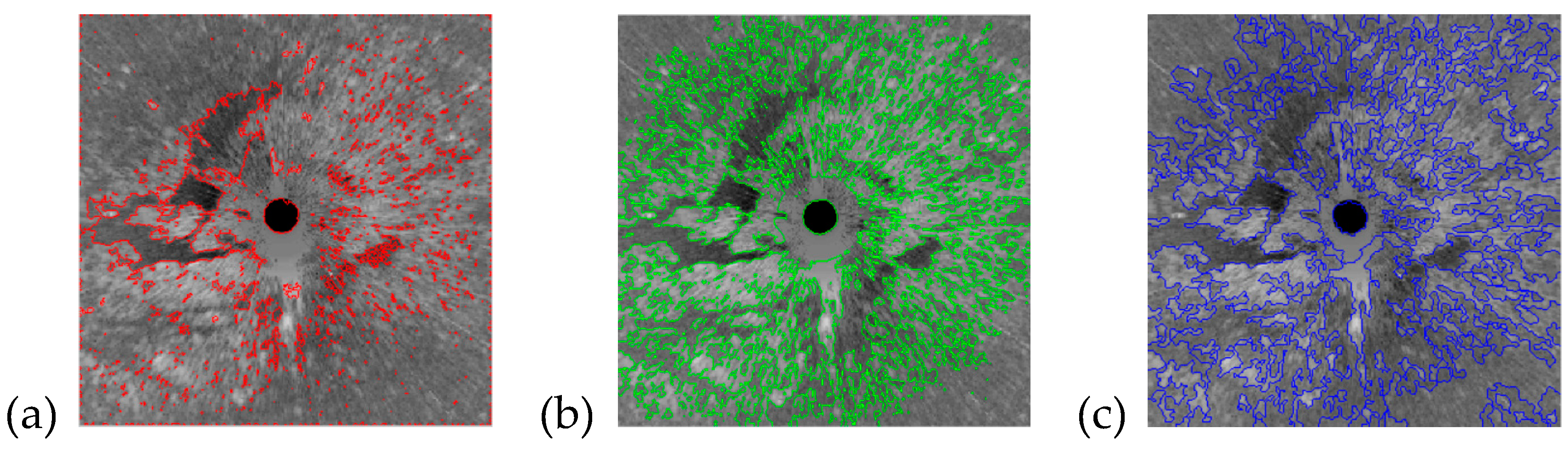
Figure 12.
Coastline segmentation results of a ship-borne radar image (collected at 08:59:20, 12 August 2015). (a) Initial contour; and (b–d) results from the LBF, LGIF, and LIF models, respectively. Parameters: λ1 = 1, λ2 = 2, σ = 5, and i (number of iterations) = 5.
Figure 12.
Coastline segmentation results of a ship-borne radar image (collected at 08:59:20, 12 August 2015). (a) Initial contour; and (b–d) results from the LBF, LGIF, and LIF models, respectively. Parameters: λ1 = 1, λ2 = 2, σ = 5, and i (number of iterations) = 5.

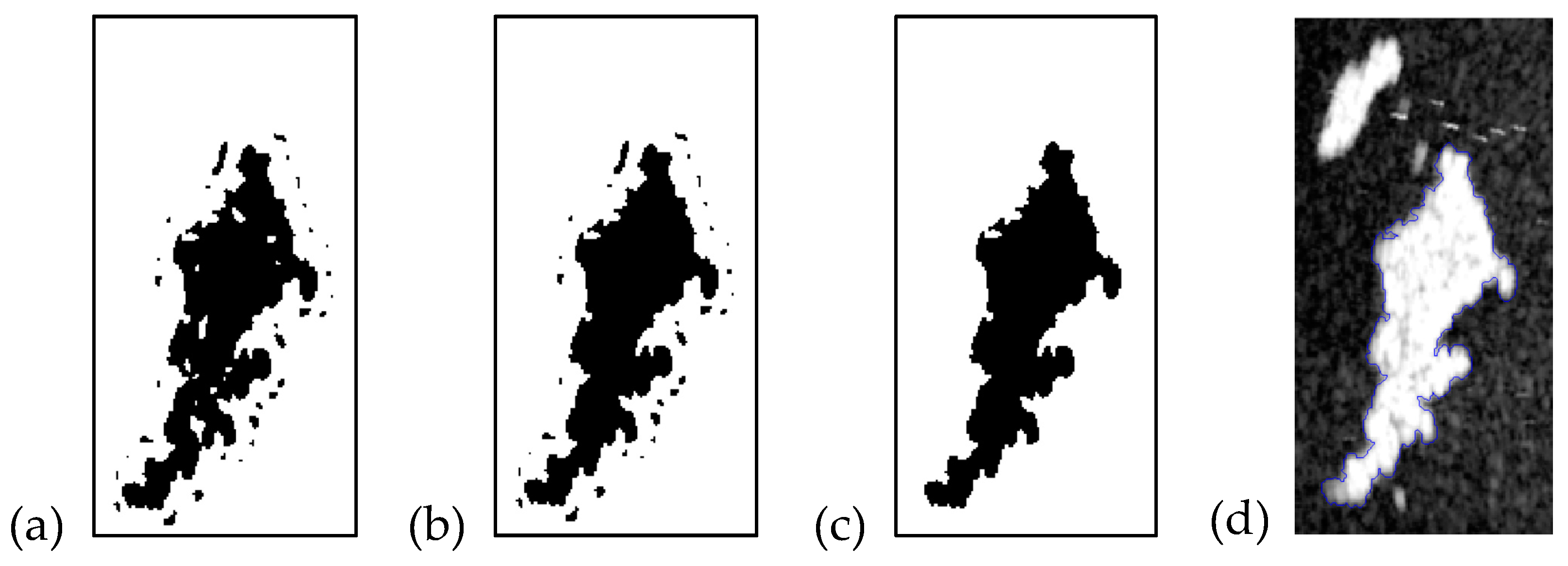
Figure 13.
Pixel area threshold method applied to Figure 12d. (a) Initial recognition result; (b) deleted interference outside the contour Tout = 50; (c) deleted interference outside the contour Tin = 30; and (d) the final contour.
Figure 13.
Pixel area threshold method applied to Figure 12d. (a) Initial recognition result; (b) deleted interference outside the contour Tout = 50; (c) deleted interference outside the contour Tin = 30; and (d) the final contour.

Figure 14.
Data samples of pre-processed images. (a–d) Pre-processed images of Figure 3.
Figure 14.
Data samples of pre-processed images. (a–d) Pre-processed images of Figure 3.

Figure 15.
Local Binary Fitting (LBF) model results: (a), (d), (g), and (k) are the pre-set contours; (b), (e), (h), and (l) show the LBF model results; and (c), (f), (i), and (m) are the final results of our model.
Figure 15.
Local Binary Fitting (LBF) model results: (a), (d), (g), and (k) are the pre-set contours; (b), (e), (h), and (l) show the LBF model results; and (c), (f), (i), and (m) are the final results of our model.

Figure 16.
Oil-spill clean-up scene images. Both (a) and (b) were obtained on 21 July 2010.

Figure 17.
Verification of thermal infrared images. The dark areas in (a,b) are oil films.

Figure 18.
Sea clutter image of calm sea surface.

Figure 19.
Results of various ACMs. (a) Pre-set contour; (b–d) LBF, Local and Global Intensity Fitting (LGIF), and Local Image Fitting (LIF) model results, respectively.
Figure 19.
Results of various ACMs. (a) Pre-set contour; (b–d) LBF, Local and Global Intensity Fitting (LGIF), and Local Image Fitting (LIF) model results, respectively.

Figure 20.
Additional LBF model results. (a–c) are the results with parameter values of λ1 = 1, λ2 = 2, σ = 2, and i = 5, 10, 20; (d–f) are the results with parameter values of λ1 = 1, λ2 = 2, σ = 3, and i = 5, 10, 20; and (g–i) are the results with parameter values of λ1 = 1, λ2 = 1, σ = 2, and i = 5, 10, 20.

Figure 21.
Additional results of various ACMs: (a–c) LBF, LGIF, and LIF model results, respectively.
Figure 21.
Additional results of various ACMs: (a–c) LBF, LGIF, and LIF model results, respectively.

Figure 22.
Comparison of segmentation results with different methods: (a–d) Results from the methods proposed by Zhu et al. [24], Liu et al. [25], Xu et al. [26], and our method, respectively.

Figure 23.
Decision matrix for effective wave area.


Table 1.
Parameters of the ship-borne radar.
| Parameter | Value |
|---|---|
| Band | X-band |
| Detection distance | 0.5/0.75/1.5/3/6/12/24 NMs |
| Range resolution | 3.75 m |
| Antenna type | Waveguide split antenna |
| Polarization mode | Horizontal |
| Horizontal detection angle | 360° |
| Rotation speed | 28–45 revolutions/min |
| Length of antenna | 8 ft |
| Pulse recurrence frequency | 3000 Hz/1800 Hz/785 Hz |
| Pulse width | 50 n/250 ns/750 ns |
Table 2.
The area of identified oil-films.
| Figure ID | Pixel Area of Oil-Films | Area of Oil-Films (m2) |
|---|---|---|
| Figure 12c | 1413 | 10,399.7 |
| Figure 12f | 883 | 6498.9 |
| Figure 12i | 418 | 3076.5 |
| Figure 12m | 1420 | 10,451.2 |
Table 3.
Contrasting terms of different Active Contour Models (ACMs).
| ACMs | LBF | LGIF | LIF | |
|---|---|---|---|---|
| Contrasting Term | ||||
| Execution time (s) | 0.547 | 0.750 | 0.072 | |
| Area of segmentation (number of pixels) | 1369 | 1225 | 1721 | |
Table 4.
Computing time (s) of LBF model with varying σ.
| i | 5 | 10 | 20 | |
|---|---|---|---|---|
| σ | ||||
| 2 | 0.425 | 0.769 | 1.367 | |
| 5 | 0.478 | 0.866 | 1.55 | |
| 10 | 0.744 | 1.252 | 2.515 | |
© 2019 by the authors. Licensee MDPI, Basel, Switzerland. This article is an open access article distributed under the terms and conditions of the Creative Commons Attribution (CC BY) license (http://creativecommons.org/licenses/by/4.0/).
Share and Cite
MDPI and ACS Style
Xu, J.; Wang, H.; Cui, C.; Liu, P.; Zhao, Y.; Li, B. Oil Spill Segmentation in Ship-Borne Radar Images with an Improved Active Contour Model. Remote Sens. 2019, 11, 1698. https://0-doi-org.brum.beds.ac.uk/10.3390/rs11141698
AMA Style
Xu J, Wang H, Cui C, Liu P, Zhao Y, Li B. Oil Spill Segmentation in Ship-Borne Radar Images with an Improved Active Contour Model. Remote Sensing. 2019; 11(14):1698. https://0-doi-org.brum.beds.ac.uk/10.3390/rs11141698
Chicago/Turabian StyleXu, Jin, Haixia Wang, Can Cui, Peng Liu, Yang Zhao, and Bo Li. 2019. "Oil Spill Segmentation in Ship-Borne Radar Images with an Improved Active Contour Model" Remote Sensing 11, no. 14: 1698. https://0-doi-org.brum.beds.ac.uk/10.3390/rs11141698
Note that from the first issue of 2016, this journal uses article numbers instead of page numbers. See further details here.