Land Surface Temperature Derivation under All Sky Conditions through Integrating AMSR-E/AMSR-2 and MODIS/GOES Observations

Abstract

Land surface temperature (LST) is an important input to the Atmosphere–Land Exchange Inverse (ALEXI) model to derive the Evaporative Stress Index (ESI) for drought monitoring. Currently, LST inputs to the ALEXI model come from the Geostationary Operational Environmental Satellite (GOES) and Moderate Resolution Imaging Spectroradiometer (MODIS) products, but clouds affect them. While passive microwave (e.g., AMSR-E and AMSR-2) sensors can penetrate non-rainy clouds and observe the Earth’s surface, but usually with a coarse spatial resolution, how to utilize multiple instruments’ advantages is an important methodology in remote sensing. In this study, we developed a new five-channel algorithm to derive LST from the microwave AMSR-E and AMSR-2 measurements and calibrate to the MODIS and GOES LST products. A machine learning method is implemented to further improve its performance. The MODIS and GOES LST products still show better performance than the AMSR-E and AMSR-2 LSTs when evaluated against the ground observations. Therefore, microwave LSTs are only used to fill the gaps due to clouds in the MODIS and GOES LST products. A gap filling method is further applied to fill the remaining gaps in the merged LSTs and downscale to the same spatial resolution as the MODIS and GOES products. With the daily integrated LST at the same spatial resolution as the MODIS and GOES products and available under nearly all sky conditions, the drought index, like the ESI, can be updated on daily basis. The initial implementation results demonstrate that the daily drought map can catch the fast changes of drought conditions and capture the signals of flash drought, and make flash drought monitoring become possible. It is expected that a drought map that is available on daily basis will benefit future drought monitoring.

1. Introduction

Land surface temperature (LST) plays a critical role in the interaction between the Earth land surface and the atmosphere by controlling the surface upwelling radiation and affecting surface energy (sensible heat and latent heat flux) exchange with the atmosphere. Thus, LST, as a key parameter for the Earth’s surface energy balance and exchange, is significant in researching the fields of climatology, hydrology, meteorology, and ecology [1,2]. LST has been widely used for environmental modeling [1,2,3], urban heat island studies [4,5,6,7], soil moisture estimate [8,9,10], derivation of evapotranspiration (ET) [11,12,13,14], and drought monitoring [15,16].

Deriving accurate satellite-based LSTs has long been an interesting and challenging research area in thermal remote sensing [17]. Significant efforts have been made throughout the past decades to derive LST from space and aircraft optical sensors, such as polar orbit sensors, like the Advanced Very-High-Resolution Radiometer (AVHRR) [18], the Moderate Resolution Imaging Spectroradiometer (MODIS) [19,20,21], and the Visible Infrared Imaging Radiometer Suite (VIIRS) [22]; and, geostationary satellites, like the Geostationary Operational Environmental Satellite (GOES) [23,24,25,26]. Optical instruments can provide good quality LST products under clear sky conditions. However, clouds affect optical sensors, like AVHRR, MODIS, VIIRS, and GOES. Meanwhile, microwave emission can penetrate non-precipitating clouds.

Passive microwave (MW) observations have been used to estimate LST since 1990 [27,28,29,30,31,32,33,34,35]. Njoku and Li [31] developed an LST algorithm while using the Advanced Microwave Scanning Radiometer (AMSR) multi-channels at 6.6, 10.7, and 18.7 GHz. Mao et al. [36,37] established a regression model between the brightness temperature (BT) of the AMSR-E bands at 18.7, 23.8, 36.5, and 89 GHz and MODIS LST products due to the difficulty of obtaining the matched ground truth for the large scale pixel (e.g., 25 km × 25 km for AMSR-E) of passive microwave data at the satellite pass. They found that the 89GHz vertical polarization is the best single band to calibrate MODIS LST, and the average bias error is about 2–3 °C in relative to the MODIS LST products. Holmes et al. [32] found that the channel with the highest correlation to LST is the 36.5 GHz, because it suffers a weaker atmospheric effect than the 89 GHz channel and weaker penetration depth effect than the lower frequency channels.

LST is a fast-response variable and thus provides proxy information at relatively high spatial resolution for the rapid changes in land surface soil moisture and crop stress conditions. Therefore, LST is an important input for the Atmosphere-Land Exchange Inverse (ALEXI) model [3], which has been used for drought monitoring and it shows promising results. The Evaporative Stress Index (ESI) that was derived from the ALEXI model describes temporal anomalies in evapotranspiration (ET), highlighting areas with abnormal states of water use across the land surface. Here, ET is retrieved via energy balance while using remotely sensed LST as the time-change signals. The LST data input into the ALEXI is obtained from the GOES. The GOES-based retrievals of LST are currently implemented with a gap-filling algorithm to estimate ET at spatial resolutions of about 4 km. The ALEXI uses LST at the morning and midmorning (1 to 1.5 h after sunrise and before local noon) as its driving input, because this is the signature in the diurnal surface temperature wave that is most closely correlated with soil moisture content [13]. Recently, it was found that the difference of MODIS daytime and nighttime LST difference (ΔT_MODIS) has a very good relationship with the GOES LST difference (ΔT_GOES) between two times at 1 to 1.5 h after sunrise and before local noon. Therefore, MODIS LST can also be implemented into the ALEX model to estimate ET at MODIS spatial resolution of 1 km.

Currently, weekly composite GOES LST is used for the input to the ALEX model, therefore, the ESI, as well as the US Drought Monitor (USDM) to remove cloud contamination and obtain a clear LST map, providing weekly drought monitoring. Recently, “flash” drought concept appears. Flash drought frequently occurred in the central and eastern United States [17]. The 2012 drought over the Northern American had the worst surface condition since the 1930s Dust Bowl [38]. The drought started in 2011, extended rapidly in 2012 (especially in June and July according to the USDM classifications), and then continued in 2013. This event was pervasive in the central regions of the United States due to the absence of rainfall in the growing season. The rapid soil moisture loss led this event as “flash drought” [39]. The flash drought event was a result of natural weather variations, with little warnings found from the traditional drought metrics or climate model simulations, unlike the common drought that is caused by external forcing like SST anomalies [40]. The flash drought event suggests that the current drought monitoring should enhance its temporal resolution, and thus daily LST data is desired.

The ALEXI requires clear-sky conditions during the time interval for obtaining the LST data and satisfying the model assumptions of the linear sensible heat rise during the morning boundary layer growth phase [14]. MODIS and GOES can provide high quality LST products under clear-sky conditions [19,20,21,23,24,25,26]. However, more than 60% of the areas in the MODIS LST products are contaminated by weather effects, especially cloud cover [41]. On the other hand, microwave sensors, such as the polar orbiting satellite sensor AMSR-EOS (AMSR-E), onboard the same Aqua satellite as the MODIS), can penetrate non-rainy clouds. The AMSR-E stopped rotating on 4 October 2011. Fortunately, a similar instrument AMSR-2 on JAXA’s GCOM-W1 spacecraft was launched on 18 May 2012, and it is currently operating. Both the AMSR-E and AMSR-2 can provide LST twice a day (the Equator crossing time 1:30 pm and 1:30 am) under all weather conditions. How to utilize the multiple instruments’ advantages is an important approach in remote sensing. Kou et al. [42] proposed blending MODIS and AMSR-E LST data by using the Bayesian Maximum Entropy (BME) method.

The main goal of this study is to develop new models for LST derivation under all sky conditions by integrating MW and optical data. We need to calibrate AMSR-E to MODIS LST and establish models between brightness temperature of AMSR-E to meet the demands of applications in the ALEXI model, and the LST from MODIS for the historical data and to calibrate AMSR-2 to GOES LST and build equations between AMSR-2 BT and GOES LST for the current data. In this study, we will conduct more intensive and comprehensive investigation for the TIR-MW LST retrieval methods and how it can be used to enhance the temporal resolution for flash drought monitoring.

2. Data and Methods

2.1. Data Used

A comprehensive data set is collected and processed in this study for deriving satellite LSTs and evaluating the data against the in situ observations. A detailed description is given in the following subsections.

2.1.1. Satellite Data

The Advanced Microwave Scanning Radiometer for the Earth Observing System (AMSR-E) is a dual-polarized passive microwave radiometer onboard Aqua that operates at the frequencies of 6.9 GHz, 10.7 GHz, 18.7 GHz, 23.8 GHz, 36.5 GHz, and 89.0 GHz [43]. The spatial resolution of the AMSR-E is higher than the previous spaceborne passive microwave radiometers in operation (from approximately 60 km at 6.9 GHz to 5 km at 89.0 GHz, with the low frequencies being obtained at 25-km resolution based on oversampling) [44].

The AMSR-2 that was on board the GCOM-W1 satellite was launched in May 2012. Similar to AMSR-E, AMSR-2 also measures the microwave emission from the Earth surface and atmosphere. AMSR-2 has seven frequencies with both vertical and horizontal polarizations when compared to AMSR-E—with an additional frequency at 7.3 GHz. AMSR-2 has approximately 62 × 35, 62 × 35, 42 × 24, 22 × 14, 19 × 11,12 × 7, and 5 × 3 km spatial resolution at 6.9 GHz, 7.3GHz, 10.65 GHz, 18.7 GHz, 23.8 GHz, 36.5 GHz, and 89.0 GHz, respectively. The low frequencies can be resampled into a 10 km resolution (Japan Aerospace Exploration Agency, 2013). The same as the AMSR-E sensor, it can acquire a set of daytime and nighttime MW data twice a day (the Equator crossing time is 1:30 p.m. for ascending pass and 1:30 a.m. for descending pass).

• The MODIS daily Aqua LST product (MYD11C1) in version 5.1, with a spatial resolution of 5 km is used in this study. Only good quality LST data with an accuracy of less than 1 K is selected.
• The MODIS land covers Climate Modeling Grid (CMG) product in version 5.1 (Short Name: MCD12C1) provides the dominant land cover types at a spatial resolution of 0.05°.
• The MODIS L3 monthly emissivity product [21], at a 0.05° resolution in version 5.1 [45], is used to estimate the broadband emissivity in this study, because it is found that daily emissivity data have many missing values, whereas the weekly data include some abnormal values.
• The Normalized Difference Vegetation Index (NDVI) data that were used in the microwave algorithm development is extracted from the MODIS 16-days NDVI composite (short name: MYD13C1), with a resolution of 0.05° [46]. The daily NDVI data used in the downscaling process were derived from the MODIS/Aqua surface reflectance product at 0.05° grid (short name: MYD09CMG) [47]. The gaps in the daily NDVI data are filled with the previously available data.
• The Geostationary Operational Environmental Satellite (GOES) monitors the weather conditions in the Unites States (U.S.). The GOES LST data used in this study, which is available at half-hour temporal resolution and 4 km spatial resolution, are derived from the GOES-13 imager observations at 3.9 µm and 11 µm channels while using the algorithms that Sun and Pinker [24] and Sun et al. [26] developed.
• The digital elevation model (DEM) data are derived from the National Elevation Dataset (NED) data [48] at a resolution of 100 m.

2.1.2. In-Situ Data

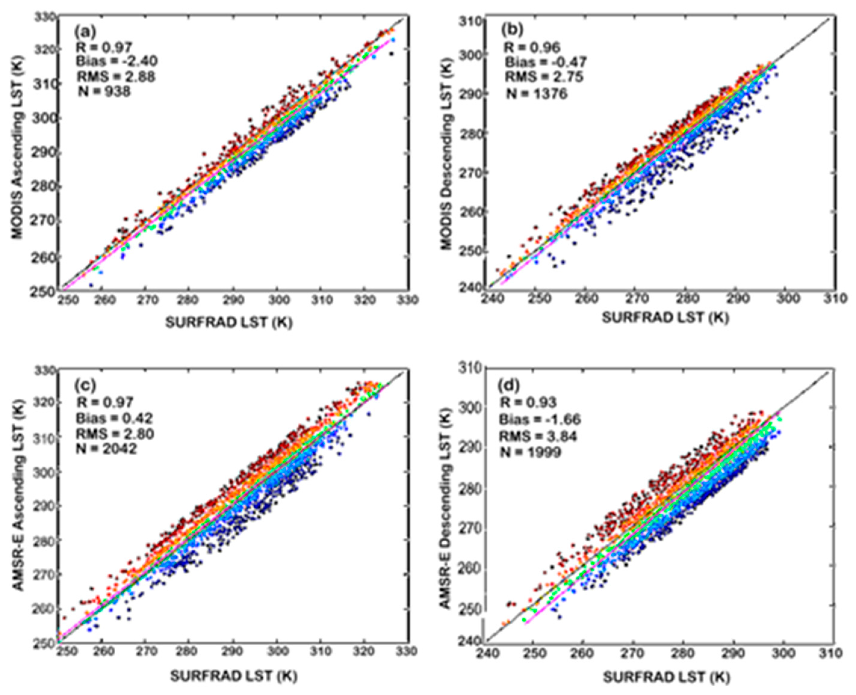
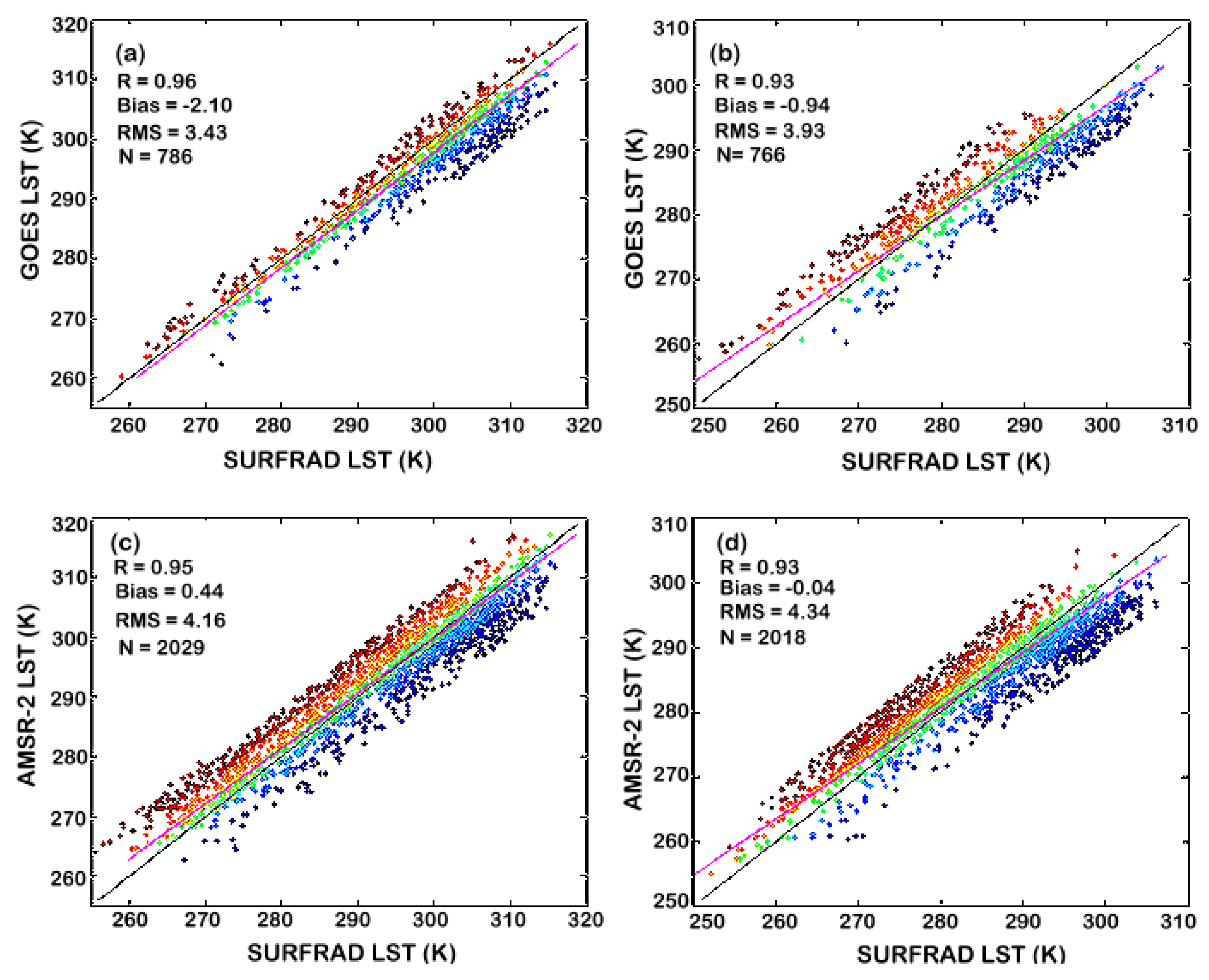
In-situ LST ground measurements are matched with the retrieved LSTs at the same time over the same location in order to validate satellite-derived LST data. The Surface Radiation Budget Network (SURFRAD) observations, which measure the surface long-wave radiation and they are an indirect measurement of LST, and are used to evaluate the LSTs that were derived from this study. A detailed description of the SURFRAD network and associated instrumentation can be found in [49].

Table 1. Surface Radiation Budget Network (SURFRAD) sites for algorithm validation.

Site No.	Site Location	Lat (N)/Lon(W)	Surface Type *
1	Bondville, IL	40.05/88.37	Crop Land
2	Fort Peck, MT	48.31/105.10	Close Shrubland
3	Goodwin Creek, MS	34.25/89.87	Deciduous Forest
4	Table Mountain, CO	40.13/105.24	Crop Land
5	Sioux Falls, SD	43.73/96.62	Grass Land
6	Pennsylvania State University, PA	40.72/77.93	Mixed Forest

* IGBP surface types.

provides brief information regarding the six SURFRAD stations that were used in this study.

The surface long-wave radiation (upwelling and downwelling radiative fluxes) data available from the SURFRAD can be converted to surface skin temperature by the following equation:

$$T_s={\left[\frac{F^{\uparrow }-\left(1-{\epsilon }_b\right)F^{\downarrow }}{{\epsilon }_b\sigma }\right]}^{\frac{1}{4}}$$

(1)

where F^↑ is the surface upwelling longwave radiation, F^↓ is the surface downwelling longwave radiation, ε_b is the surface broadband emissivity, and σ is the Stefan–Boltzmann constant.

The broadband emissivity (ε_b) in Equation (1) can be estimated from the MODIS spectral emissivity while using narrowband to broadband conversion method [50], as follows:

$${\epsilon }_b=0.2122{\epsilon }_{29}+0.3859{\epsilon }_{31}+0.4029{\epsilon }_{32}$$

(2)

where ε₂₉, ε₃₁, and ε₃₂ are the spectral emissivity of MODIS bands 29, 31, and 32, respectively.

2.2. Methods

2.2.1. Physical Basis for Remote Sensing of LST from Passive Microwave

The physical basis for LST retrieval from passive microwave observations is based on the radiative transfer theory. The radiance that was received at remote sensor level includes the radiance that was emitted by the Earth surface and the atmospheric effects. The radiative transfer equation for passive microwave remote sensing of LST can be expressed, as follows [36,37]:

$$B_f\left(T_f\right)={\tau }_f\left(\theta \right){\epsilon }_f{B}_f\left(LST\right)+{\tau }_f\left(\theta \right)(1-{\epsilon }_f)B_f\left({T^{\downarrow }}_a\right)+B_f({T^{\uparrow }}_a)$$

(3)

where T_a^↓ is the downward atmospheric brightness temperature, and T_a^↑ is the upward atmospheric brightness temperature, T_f is the brightness temperature of frequency f, τ_f is the atmospheric transmittance in frequency f at viewing direction θ (zenith angle from nadir), and ε_f is the ground emissivity. B_f (LST) is the ground radiance, and B_f(T_a^↓) and B_f(T_a^↑) are the downwelling and upwelling path radiances, respectively.

Fily et al. [51] found an empirical linear relationship for emissivity between vertical and horizontal polarizations: ε_V = aε_H + b, where ε_V/H stands for surface emissivity at vertical/horizontal polarization, respectively, and a and b are the linear regression coefficients. Therefore, LST can be derived:

$$LST=\left[T_{b_v}-a{T}_{b_H}-\left(1-b-a\right){\tau }_f\left(\theta \right){T^{\downarrow }}_a-\left(1-a\right){T^{\uparrow }}_a\right]/[b{\tau }_f\left(\theta \right)]$$

(4)

where T_b is for brightness temperature and subscripts V and H represent vertical and horizontal polarization, respectively. Several algorithms were selected here for comparison in order to develop good LST algorithms for passive microwave sensors AMSR-E and AMSR-2.

2.2.2. Algorithms for Retrieving LST from Passive Microwave Data

In this study, we proposed a new five-channel algorithm to derive LST from microwave observations (LST_m) by utilizing the AMSR-2 five channels at 6.9, 18.7, 23.8, 36.5, and 89 GHz in both the vertical and horizontal polarizations. The new proposed five-channel algorithm is also compared with the two previously published microwave LST algorithms:

The Single-Channel Algorithm with the 36.5 V GHz

The 36.5 GHz is considered to be the most appropriate MW channel for temperature retrieval [32], but is often invalid in wet seasons due to the scattering effect of rain droplets [52].

LST_m = β₁ + β₂T_36.5V

(5)

where β₁ and β₂ are regression coefficients.

The Four-Channel Algorithm

Mao et al. [36,37] thought: (1) T_36.5V is the primary channel to retrieve LST; (2) The brightness temperature difference at the 36.5 GHz and 23.8 GHz channels in vertical polarization (T_36.5V–T_23.8V) is utilized to attenuate the influence of atmospheric water vapor; (3) T_36.5V–T_18.7H can compensate for the influence of surface water, and, (4) T_89V can decrease the average influence of atmosphere. They used the following equation:

LST_m = B₀ + B₁ T_36.5V + B₂ (T_36.5V–T_23.8V) + B₃ (T_36.5V–T_18.7H) + B₄ T_89V

(6)

where T refers to brightness temperature, the subscripts refer to frequencies in GHz at different bands, B₀, B₁…B₄ are the regression coefficients.

A Proposed New Five-Channel Algorithm

In this study, we utilize five channels at 6.9, 18.7, 23.8, 36.5, and 89 GHz in both the vertical and horizontal polarizations, and microwave data is calibrated to optical data. Since the time for the two types of sensors may be different, the time of microwave sensor UTC is especially added to count the time difference between the two sensors.

LST_m = C₀ + C₁ (T_6.9V–c₁T_6.9H) + C₂ (T_36.5V–c₂T_36.5H) + C₃ (T_23.8V–c₃T_23.8H) + C₄ (T_18.7V–c₄T_18.7H) + C₅ (T_89V–c₅T_89H) + C₆ UTC

(7)

where T refers to brightness temperature, the subscripts refer to frequencies in GHz at different bands, UTC is the UTC time of the microwave sensor, and C₀, C₁…C₆, c₁…c₅ are the regression coefficients.

2.3. Regression Tree Algorithm

Chen et al. [41] stratified the regression models, according to the intervals of Microwave Polarization Difference Index (MPDI). Sun et al. [26] introduced the regression tree (RT) methods to stratify the regression models for LST retrieval, because the RT [53] method offers a robust tool for handling nonlinear relationships within complex data sets. The RT was adopted to develop an operational LST algorithm that uses a set of independent parameters (in this case, at-sensor brightness temperatures; satellite and solar zenith angles; and, surface emissivity) to recursively split a dependent variable (in this case, LST) into different subsets that minimize the errors [26].

An alternative approach to nonlinear regression is to sub-divide the space into smaller regions to which simple models can be fitted, unlike traditional linear regression, which is a global model where there is a single predictive formula holding over the entire data-space unless the manual separation of different sub-divisions is performed. Regression trees use the tree to represent the recursive partition. Each of the terminal nodes or leaves of the tree represents a cell of the partition to which a simple model is attached; the simple model only applies to that cell.

As a data mining tool, the Regression Tree (RT) can provide a flexible and robust analytical method for identifying the relationships between complex environmental data [35]. The regression tree presents a clear, logical model that can be easily understood. The RT program constructs an unconventional type of tree structure, with the tree leaves containing linear regression models. The RT techniques can help us to automatically identify threshold values and rules. It is possible to discern the conditions that lead to a relationship within computer-determined subsets of the data by applying rule induction techniques. RT techniques, such as the M5P, are a powerful tool for generating rule-based models that balance the need for accurate prediction [54].

The implementation of the regression tree algorithm is performed, as follows. Two samples of matched satellite pixel-truth are taken from the data sets. One sample is used for training the regression tree, and the other sample is used for testing. In this way, the over fitting problem should be avoided. The regression tree output yields an LST regression model that is based on training pixels present in each node. The predicted LST values can be determined by applying these linear models for each node.

2.4. Gap Filling and Downscaling Method

In this study, we do not fill the missing values based on previous days since LST is a fast changing variable. Instead, we assume that each gap pixel relies on its neighbours horizontally, vertically and diagonally. Thus, the value of the gap pixel can be interpolated by its neighbours, from up and down, from left and right. Some TIR LSTs can be available inside the MW passing gaps, and they can partially fill the gaps, and also help to reduce the errors of the interpolation.

However, such a regular gap-filling method cannot catch the observations when there is a big gap, as shown in Figure 1d. Accordingly, we propose a gap-filling method based on the Geographically Weighted Regression (GWR). In addition to the gap filling function, the coarse spatial resolution of the microwave observation, such as 25 km for the AMSR-E and 10 km for the AMSR-2, can also be downscaled to the same spatial resolution of the thermal LST products, like 5km for MODIS LST and 4 km for GOES LST. The traditional GWR algorithm has been used to interpolate the regression coefficients and the residual term [55]. This process requires two auxiliary data: NDVI and elevation. The daily NDVI data is derived from the MODIS/Aqua surface reflectance product at 0.05° grid (short name: MYD09CMG) [30]. The elevation data is obtained from the National Elevation Dataset (NED) data [48], at a resolution of 100 m, and resampled to 5 km via bi-cubic interpolation, as well as 25 km.

The specific procedures are as follows:

(1)

Aggregate NDVI and DEM to microwave resolution (25 km for AMSR-E and 10 km for AMSR-2). Here, we take the AMSR-E and MODIS as an example, NDVI^5km and DEM^5km denote the auxiliary variables at the MODIS pixel resolution, whereas NDVI^25km and DEM^25km represent the aggregated auxiliary variables at the AMSR-E pixel resolution.

(2)

Establish the non-stationary relationship between the AMSR-E 25 km LST with the same spatial resolution auxiliary data:

LST^25km = a₀^25km(x,y) + a₁^25km(x,y) NDVI^25km + a₂^25km(x,y) DEM^25km + ε^25km

(8)

Equation (8) shows the non-stationary relationship that is to be built at coarse microwave resolution between the microwave LST (MLST) (here is for AMSR-E) and the aggregated thermal LST (here is for MODIS) with the auxiliary data.

(3)

Estimate the regression coefficients a₀(x,y), a₁(x,y), a₂(x,y), and the error term ε via Gaussian distance weighting at the coarse microwave resolution.

(4)

Apply the regular gap-filling algorithm to both MODIS LST and AMSR-E LST, so that the first gap-free observations can be obtained.

(5)

The bi-cubic interpolation is used to interpolate the regression coefficients and the residual at coarse microwave resolution to MODIS 5km resolution a₀^5km (x,y), a₁^5km(x,y), a₂^5km(x,y), and error term ε^5km.

(6)

The final downscaled LST at 5 km resolution can be calculated while using the auxiliary variables (NDVI and DEM) at 5 km resolution in conjunction with the regression coefficients and the residual term at 5 km m resolution:

LST^5km = a₀^5km(x,y) + a₁^5km(x,y) NDVI^5km + a₂^5km(x,y) DEM^5km + ε^5km

(9)

Equation (9) shows how microwave LST can be downscaled to the same resolution of thermal LST (e.g., 5 km for MODIS in this study) that were based on the GWR.

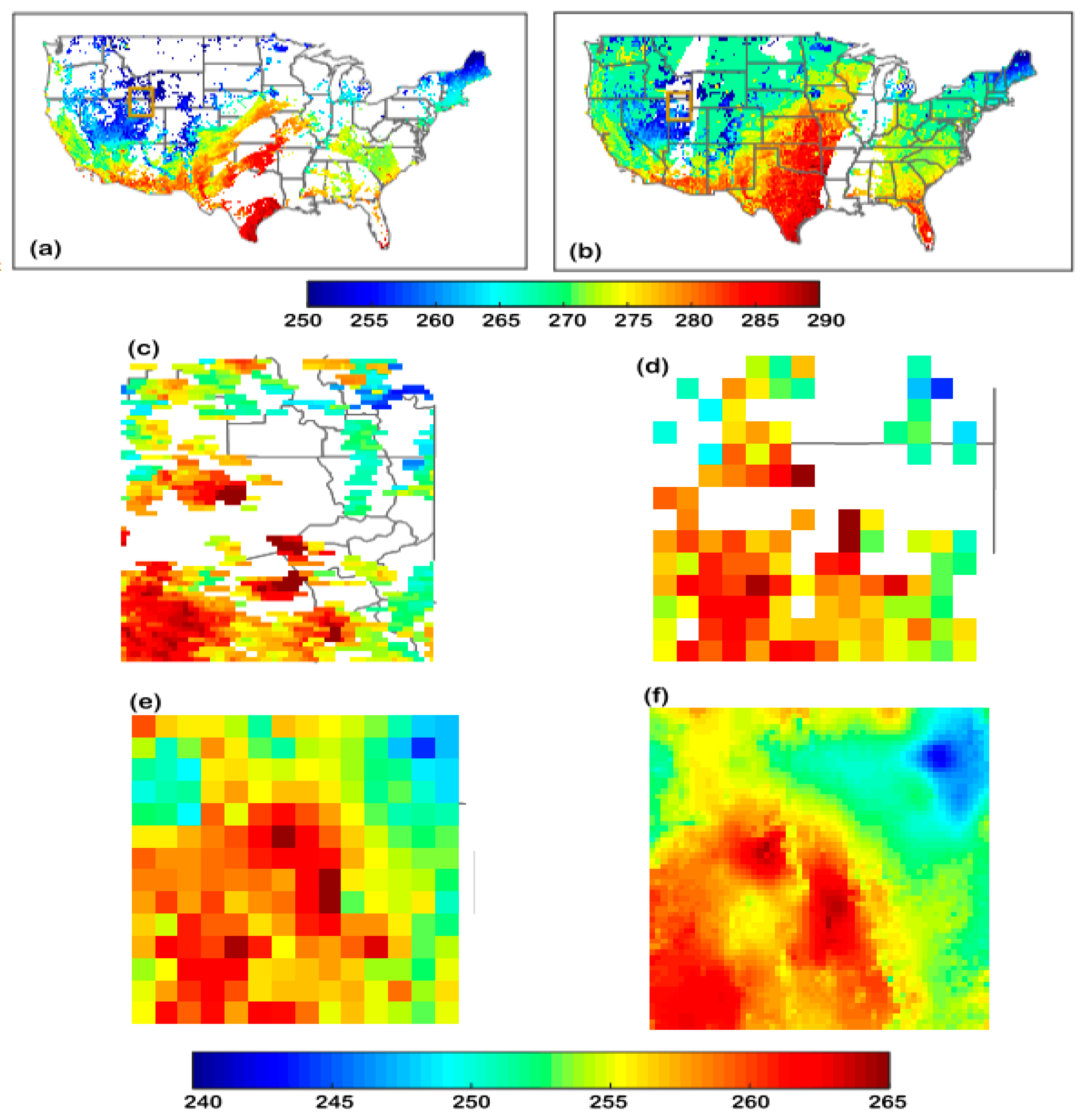
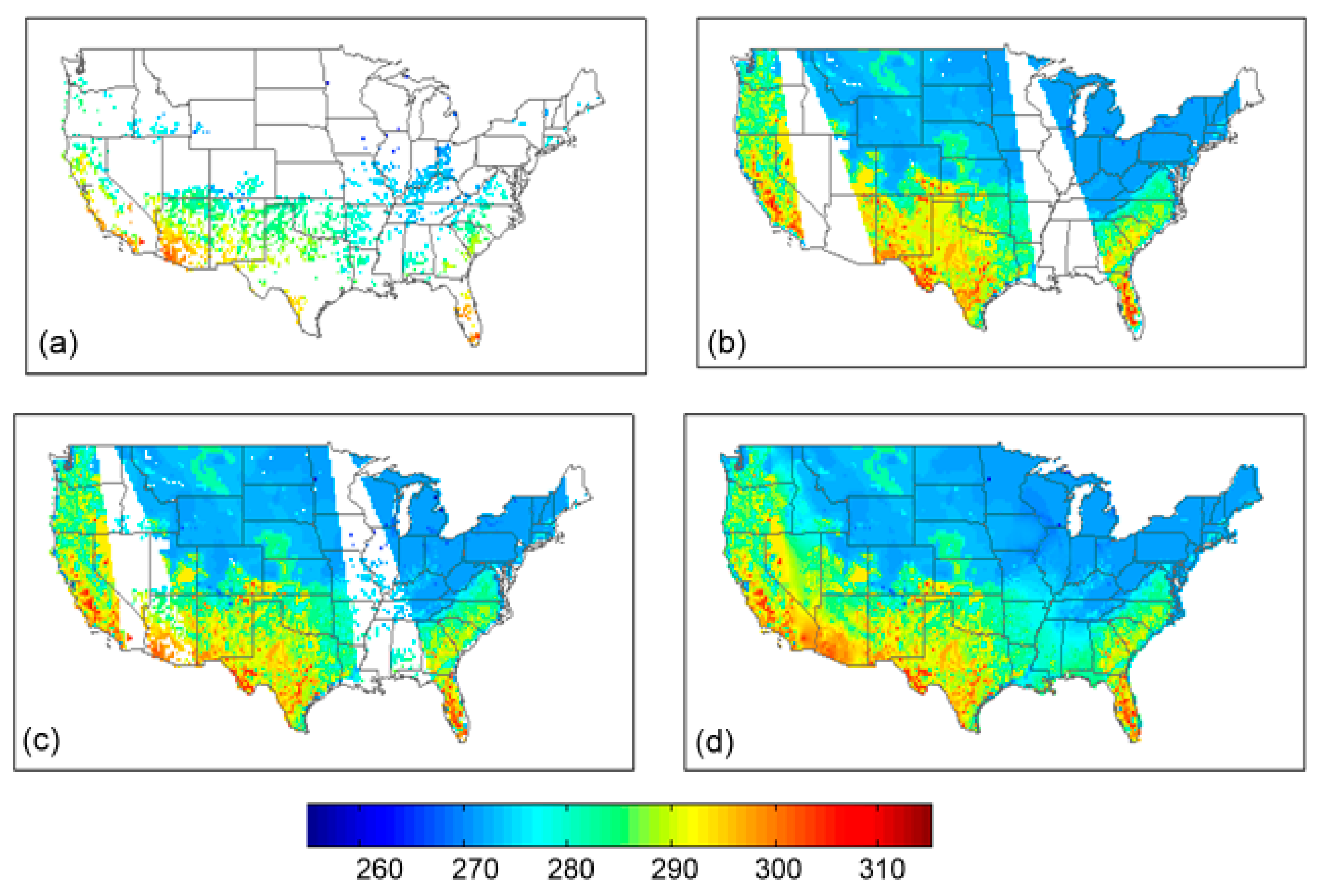
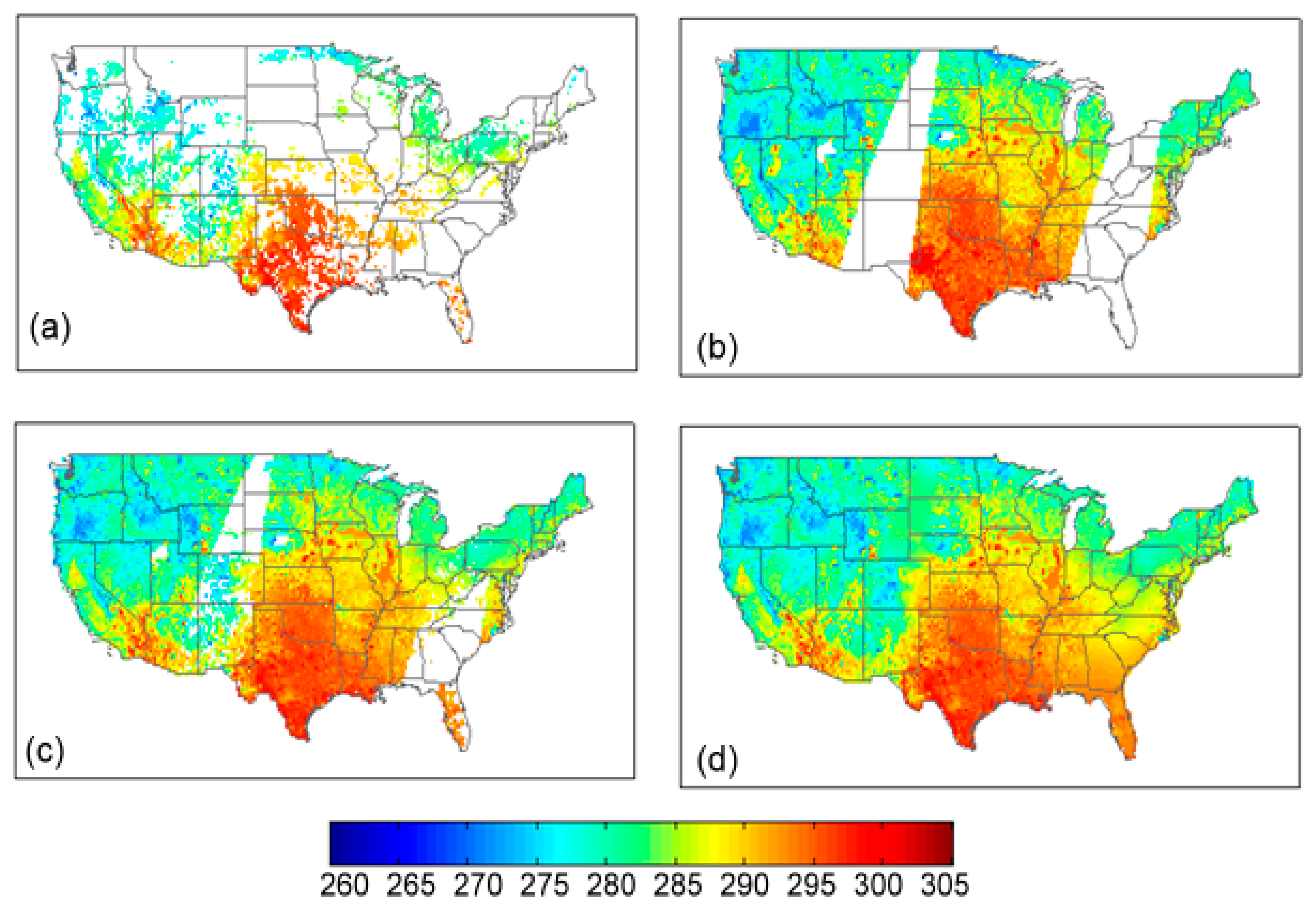
Figure 1 demonstrates an example for the gap filling and downscaling method. Figure 1a shows the original MODIS LST, Figure 1b is the merged LST that are based on MODIS and AMSR-E. We selected a zoom region to demonstrate the effects of the gap filling and downscaling method, as shown in Figure 1a,b; Figure 1e shows the result using the regular gap-filling algorithms, and the error is quite large within the big gaps. Figure 1f is the result after applying the GWR-based gap-filling algorithm.

The GWR-based interpolation (Figure 1f) outperforms the regular gap filling method (Figure 1e). In addition to gap filling, the GWR based method can simultaneously downscale the merged LST at coarse spatial resolution (25 km here) to the same spatial resolution of the thermal LST product (5 km here). This process is time consuming. The more MODIS observations can be available inside the MW gaps; the more accurate LST can be obtained.

3. Results

3.1. Results from the Calibrations

3.1.1. Results from the AMSR-E to MODIS Calibration

The MODIS LST data were aggregated to 25 km, the same resolution as the AMSR-E. Only high quality LST data with standard deviation less than 1 K are used for training the coefficients in Equations (1)–(6).

The above algorithms were then applied to the real AMSR-E observations. The LST retrieved from the AMSR-E are compared with the MODIS LST product. Correlation coefficients, the mean absolute errors (MAE), and Root Mean Square (RMS) error in relative to MODIS LST products are used to evaluate the retrieval results of the models.

Implementation of the Single-Channel Algorithm

Table 2. LST derived from AMSR-E Ascending data with the single-channel algorithm in relative to MODIS LST in daytime.

Seasons	Correlation Coefficient	MAE (K)	RMS (K)	Sample Number
Spring	0.89	4.73	5.99	215,184
Summer	0.70	4.56	6.44	348,823
Fall	0.67	4.45	6.54	341,448
Winter	0.83	4.22	5.42	168,043

and

Table 3. LST derived from AMSR-E Descending data with the single-channel algorithm in relative to MODIS LST in nighttime.

Seasons	Correlation Coefficient	MAE (K)	RMS (K)	Sample Number
Spring	0.82	5.03	6.28	139,793
Summer	0.75	3.56	5.34	255,269
Fall	0.61	3.89	5.23	253,139
Winter	0.74	4.51	6.01	105,963

list the implementation results for the single-channel algorithm. From Table 2, regarding the daytime results with the AMSR-E ascending data, we can see the average mean absolute errors (MAE) are about 4.5 K with the single frequency (band). The MAEs during nighttime are about 4 K and show a little bit better than those during the day time. This may be because the influence of the soil water and atmosphere during night time is less than that during the daytime. The results using only one frequency (band) indicate a root mean square error of about 6 K and average absolute error of about 4.5 K, which may be too big to meet our application requirements.

Implementation of the Four-Channel Algorithm

The four-channel algorithm that Mao et al. proposed [20,21] is also implemented to the real AMSR-E data and compared with the MODIS LST product. As shown in

Table 4. LST derived from the AMSR-E ascending data with the four-channel algorithm. [20] vs. MODIS LST product.

Seasons	Correlation Coefficient	MAE (K)	RMS (K)	Sample Number
Spring	0.90	3.21	4.12	215,184
Summer	0.88	3.35	4.32	348,823
Fall	0.90	2.89	3.87	341,448
Winter	0.93	2.43	3.02	168,043

and

Table 5. LST derived from the AMSR-E descending data with the four-channel algorithm [36] vs. MODIS LST product.

Seasons	Correlation Coefficient	MAE (K)	RMS Error (K)	Sample Number
Spring	0.89	2.21	3.27	139,793
Summer	0.92	2.03	2.40	255,269
Fall	0.93	1.85	2.34	253,139
Winter	0.87	2.43	3.27	105,963

, the results are similar to those from Mao et al. [20,21]. The mean absolute error (MAE) is about 2–3 K and the RMS error is about 3–4 K during daytime and the MAE is about 2 K, and RMS error is about 2.5 K during night time in relative to the MODIS LST product.

Implementation of the Proposed Five-Channel Algorithm

As shown in

Table 6. LST derived from the AMSR-E ascending data with the proposed new five-channel algorithm, compared with the MODIS LST product during daytime.

Seasons	Methods	Correlation Coefficient	MAE (K)	RMS (K)	Sample Number
Spring	L	0.92	2.95	3.95	215,184
	RT	0.99	0.16	0.83
Summer	L	0.90	3.32	4.38	348,823
	RT	0.99	0.70	0.84
Fall	L	0.91	2.92	3.98	341,448
	RT	0.99	0.70	0.78
Winter	L	0.95	2.25	2.99	168,043
	RT	0.99	0.63	0.46

and

Table 7. LST derived from the AMSR-E descending data with the proposed new five-channel algorithm, as compared with the MODIS LST product during nighttime.

Seasons	Methods	Correlation Coefficient	MAE (K)	RMS (K)	Sample Number
Spring	L	0.89	2.25	3.02	139,793
	RT	0.99	0.33	0.43
Summer	L	0.91	1.88	2.55	255,269
	RT	0.99	0.41	0.52
Fall	L	0.94	1.83	2.44	253,139
	RT	0.99	0.46	0.57
Winter	L	0.88	2.52	3.35	105,963
	RT	0.99	0.39	0.64

, the five-channel algorithm, as represented by Equation (7) by using the 6.9, 18.7, 23.8, 36.5, and 89 GHz in both vertical and horizontal polarizations, show some improvements to four-channel algorithm (Table 4 and Table 5), especially during autumn season during daytime, but no improvements during night time.

If we use regression tree (RT) method, the algorithm can be significantly improved. The mean errors or accuracies can be reduced from about 2–3 K with linear regression (L) to less than 1 K with the RT and RMS errors can be reduced from 3–4 K with linear regression (L) to less than 1 K with the RT and the correlations can be increased to 0.99 from about 0.90 with linear regression (L).

3.1.2. Results from the AMSR-2 to GOES Calibration

The five-channel algorithm is also applied to real AMSR-2 data and compared with the GOES LST products [10]. During daytime (

Table 8. LST derived from the AMSR-2 Ascending data with five-channel algorithm, as compared with the GOES LST at 1.5 h before noon.

Seasons	Methods	Correlation Coefficient	Mean Absolute Error (K)	Root Mean Squared Error (K)	Total Number of Instances
Spring	L	0.93	2.96	3.83	382,965
	RT	0.985	1.18	1.64
Summer	L	0.91	3.22	4.14	757,026
	RT	0.981	1.21	1.70
Fall	L	0.92	2.88	3.70	897,344
	RT	0.990	1.048	1.44
Winter	L	0.92	2.54	3.29	203,571
	RT	0.990	0.912	1.27

), the mean absolute errors are about 2–3 K with the linear regression (L) method, 1–1.5 K with the regression tree (RT) method, and the RMS errors are about 3–4 K from the linear regression and about 1.5 K from the RT method, and the correlation coefficients are about 0.9–0.95 from linear regression and about 0.98 from the RT method. During nighttime (

Table 9. LST derived from the AMSR-2 descending data with five-channel algorithm, as compared with the GOES LST at 1.5 h after sunrise.

Seasons	Methods	Correlation Coefficient	Mean Absolute Error (K)	Root Mean Squared Error (K)	Total Number of Instances
Spring	L	0.84	2.63	3.38	159,725
	RT	0.982	0.881	1.25
Summer	L	0.84	2.33	3.07	550,810
	RT	0.977	0.815	1.17
Fall	L	0.87	2.18	2.87	613,528
	RT	0.986	0.841	1.16
Winter	L	0.82	2.83	3.86	195,493
	RT	0.982	0.902	1.29

), the mean accuracies are about 2.5 K and RMS errors are about 3 K from the linear regression, and the MAEs are reduced to about 1 K, and RMS errors are reduced to about 1–1.5 K from the RT method.

The rules and regression models obtained from the RT machine learning or training for the proposed new five-channel algorithm with the auxiliary data are applied to the real AMSR-E and AMSR-2 observations since the RT method shows significant improvement over the traditional linear regression method.

3.2. Results from the Validation against Ground Observations

Examples for the evaluation results against the SURFRAD ground observations are also presented in Figure 2 for MODIS and AMSR-E for the year of 2008 and Figure 3 for GOES and AMSR-2 for the year of 2015. For the MODIS LST product, the mean bias is −2.40 K during daytime and −0.47 K during nighttime, the RMS errors are 2.88 K during daytime and 2.75 K during nighttime, and the correlation coefficient (R) is 0.97 during daytime (ascending pass) and 0.96 during nighttime (descending pass). For LST that were derived from the AMSR-E data, the bias is 0.42 K during daytime and −1.66 K during nighttime; the RMS error is 2.80 K during daytime and 3.84 K during nighttime, and the correlation is about 0.97 for the ascending and 0.93 for the descending data.

For the GOES LST product, the bias is −2.10 K, the RMS is 3.43 K, and correlation is 0.96 for the time at 1.5 h before the noon, and the bias is −0.94 K, the RMS is 3.93 K, and the correlation is 0.93 for the time at 1.5 h after the sunrise. For LSTs that were derived from the AMSR-2 observations, the bias is 0.44 K, the RMS error is 4.16 K, and correlation is 0.95 for the ascending data; the bias is −0.04 K, the RMS error is 4.34 K, and the correlation is 0.93 for the descending data. We can see, in general, LST from thermal IR measurements, such as MODIS and GOES, have higher correlations and they are still better than those from microwave sensors, such as AMSR-E and AMSR-2. Therefore, for clear sky conditions, we still use thermal IR data, only under cloudy conditions, we use microwave data.

3.3. Results from the Implementation to the Real Observations

Figure 2 and Figure 3 shows the validations of LSTs that are derived from the real microwave observations against the ground observations and compared with the MODIS and GOES LST products. Here, we show some examples for the spatial distributions of the implementations to the real observations.

Figure 4 and Figure 5 demonstrate examples of MODIS LST product (a), LST derived from the AMSR-E observation (b), the merged AMSR-E LST and MODIS LST, in which the LSTs are obtained from MODIS product under clear conditions, while under cloudy conditions, LST are derived from the AMSR-E measurements (c); MODIS LSTs can help to fill some pass gaps in the AMSR-E observations, there are still some gaps left, so we applied the GWR-based gap filling method to fill the gaps, as shown in (d). We can see there may be a lot of areas without data in the MODIS LST products on daily basis, while microwave, like the AMSR-E, can fill the gaps due to clouds, and give a more complete picture.

Figure 6 and Figure 7 demonstrate the GOES LST product at the original 4 km resolution (a), the AMSR-2 LST at 10 km resolution derived from the proposed new five channel algorithm with the RT implementation (b), the merged GOES and AMSR-2 LST at 10 km resolution, where there is some cloud contamination in GOES LST; the integrated GOES and AMSR-2 LST with the GWR based algorithm being applied to fill the gaps and also downscale to the same 4 km resolution as the GOES LST product (d).

As demonstrated in Figure 4, Figure 5, Figure 6 and Figure 7a, there are a lot of gaps or missing values due to clouds in the daily MODIS or GOES LST. Only a multi-day composite can get a clear LST map, so the current ESI are updated weekly. Microwave observations can be used to fill the gaps due to clouds in the thermal IR LST, since microwave sensor can penetrate clouds and observe the Earth surface. The microwave observations are firstly calibrated to thermal IR (MODIS and GOES, here) LST, merged with the IR observations to fill the gaps due to clouds in the IR LST, and then downscaled to the same spatial resolution as the IR LST. With the integrated IR and MW LSTs, spatial continuously distributed LST can be obtained on a daily basis, as shown in Figure 4, Figure 5, Figure 6 and Figure 7d.

With the daily integrated IR and MW LST, a drought index, like the ESI, can be updated on daily basis without gaps due to clouds. Figure 8 demonstrates an example. When compared with the current ESI, which is updated weekly, and the USDM map, which provides weekly drought monitoring, in general, the daily drought maps agree with the USDM drought classifications, and meanwhile can catch the flash changes of drought conditions.

4. Discussion

Optical instruments, like MODIS and GOES, can provide high quality LST products under clear sky conditions [18,19,20,21,22,23,24,25,26], however more than 60% of the areas in the MODIS LST products are contaminated by weather effects, especially cloud cover [41]. Passive microwave (e.g., AMSR-E and AMSR-2) can penetrate non-rainy clouds, but usually with more coarse spatial resolution than optical sensors. How to utilize multiple instruments’ advantages is an important approach in remote sensing.

Currently, the ESI, as well as the widely used USDM drought map, provides weekly drought monitoring. While, recently, “flash” drought events frequently occurred in the central and eastern United States, and suggest that the current weekly drought monitoring should enhance its temporal resolution, thus daily LST is desired. In this study, a new five-channel algorithm is proposed to derive LST from the microwave AMSR-E and AMSR-2 observations by calibrating to the thermal MODIS and GOES LST products. A GWR-based method is further applied to fill the remaining gaps and to downscale to the same spatial resolution as the thermal LST products. Nevertheless, the results will mostly come from the interpolation if there are not enough valid thermal and/or MW observations in the merged LST data, thus the accuracy shall be limited. For this kind of situation, a new super resolution technique is adopted for further improvement, and the details will be described in another paper [56]. With this new technology, further improvements can help to fill the methodological and data gaps. Nevertheless, the downscaling processes may be time consuming.

With the method proposed here, drought indices using LST as an input can be updated daily without gaps. In general, the daily drought map agrees with the current ESI and the USDM drought classifications, and meanwhile it can catch the fast changes of drought conditions and thus capture the early signals of flash drought. The drought index that was derived with the integrated LST shall be comprehensively compared with other methods, like the vegetation temperature condition index (VTCI) [15,16], the current ESI [3], etc. However, it is out of the scope of this study. The main goal of this study is to develop new methods for daily LST derivation under all sky conditions by integrating MW and thermal LST data. It is expected that daily LSTs that were obtained in this way with continuous spatial distribution can help soil moisture, surface sensible and latent heat fluxes, ET, and drought index, like the ESI, estimation on daily basis under nearly all sky conditions and benefit future drought monitoring, and improve the urban heat island and environmental modeling studies. The spatial continuous daily LST can also help in the calibration and evaluation where there is no ground truth data to calibrate and compare.

More validations or evaluations to the integrated IR and MW LST will be conducted, and extensive tests regarding its implementation to the ALEXI model shall be performed. The integrated LST shall be implemented for future operational use if the results are promising and robust.

5. Summary

As clouds obscure thermal infrared LST observations, the microwave sensor can penetrate most non-rainy clouds and observe the Earth surface. How to utilize the advantages of multi-sensor observations to overcome each other’s shortcoming is still challenging in remote sensing. In this study, a new five-channel algorithm is proposed to derive LST from the microwave AMSR-E and AMSR-2 observations by calibrating to the thermal MODIS and GOES LST products. The proposed new five-channel algorithm is compared with the previously published single channel algorithm and four-channel algorithm, and it shows some improvements. Moreover, a supervised machine learning technique, the regression tree (RT), was introduced to determine the stratification of the regression coefficients under different conditions. The accuracies from the training with the RT were compared with those using the traditional regression method. It was found that the RT method further outperforms the traditional linear regression method.

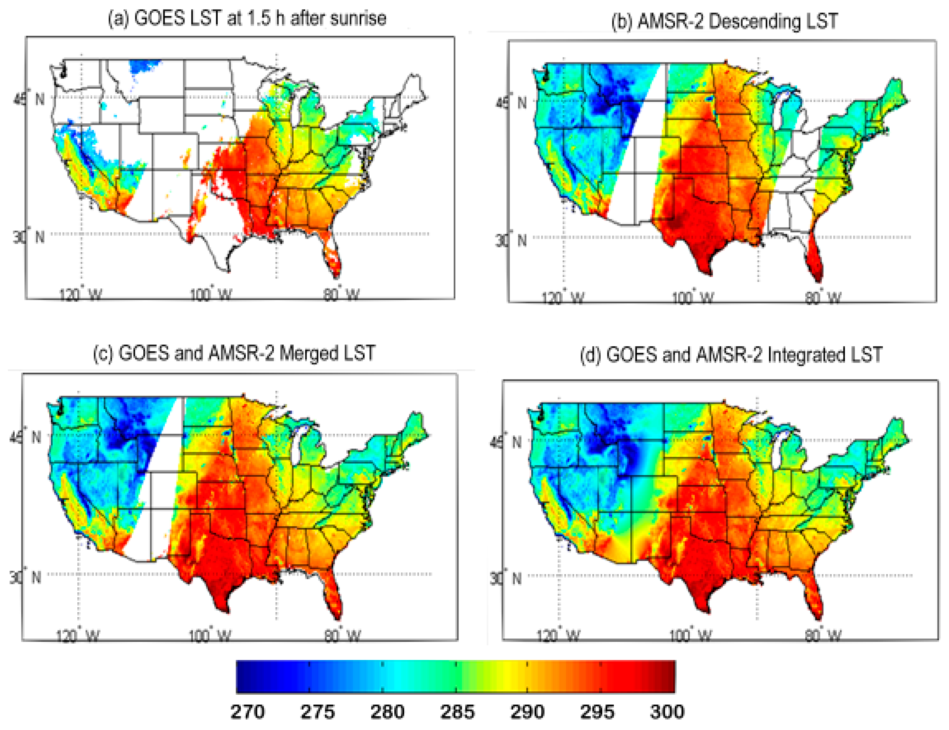
The results indicate that, in general, LST from the thermal IR measurements, such as the MODIS and GOES, have better performance than those from microwave sensors, such as the AMSR-E and AMSR-2. Therefore, thermal IR data are still used for clear sky conditions, and microwave data are only utilized to fill the gaps due to clouds in the thermal data. The thermal LST products can help to fill some pass gaps of the microwave sensors in the merged LST data, but some gaps are still left. A GWR-based method is further applied to fill the remaining gaps and to also downscale to the same spatial resolution as the thermal LST products. In this way, with the newly proposed methodology, daily clear LST can be obtained at the same spatial resolution as the thermal LST products.

Currently, the ESI is updated weekly because thermal infrared LST products are affected by clouds, and only multi-day composite can get a clear LST map. Recently, the frequent “flash” drought events that occurred in the central and eastern U.S. suggest that the current weekly drought monitoring should enhance its temporal resolution, thus daily LST data is desired. In this study, microwave observations are utilized to fill the gaps due to clouds in the thermal IR LST to generate daily LST map without gaps. Microwave observations are firstly calibrated to thermal IR (MODIS and GOES here) LST with the new developed five-channel algorithm, and then merged with the IR observations. The GWR method is applied to further downscale the merged LST to the same spatial resolution as the IR LST. With the integrated IR and MW LST obtained in this way, a drought index, like the ESI, can be updated daily and make flash drought monitoring become possible.

References

1. Kustas, W.; Anderson, M. Advances in thermal infrared remote sensing for land surface modeling. Agric. For. Meteorol. 2009, 149, 2071–2081. [Google Scholar] [CrossRef]
2. Anderson, M.C.; Norman, J.M.; Kustas, W.P.; Houborg, R.; Starks, P.J.; Agam, N. A thermal-based remote sensing technique for routine mapping of land-surface carbon, water and energy fluxes from field to regional scales. Remote Sens. Environ. 2008, 112, 4227–4241. [Google Scholar] [CrossRef]
3. Anderson, M.C.; Norman, J.M.; Diak, G.R.; Kustas, W.P.; Mecikalski, J.R. A two-source time-integrated model for estimating surface fluxes using thermal infrared remote sensing. Remote Sens. Environ. 1997, 60, 195–216. [Google Scholar] [CrossRef]
4. Voogt, J.A.; Oke, T.R. Thermal remote sensing of urban climates. Remote Sens. Environ. 2003, 86, 370–384. [Google Scholar] [CrossRef]
5. Estoque, R.C.; Murayama, Y. Monitoring surface urban heat island formation in a tropical mountain city using Landsat data (1987–2015). ISPRS J. Photogram. Remote Sens. 2017, 133, 18–29. [Google Scholar] [CrossRef]
6. Stathopoulou, M.; Cartalis, C. Downscaling AVHRR land surface temperatures for improved surface urban heat island intensity estimation. Remote Sens. Environ. 2009, 113, 2592–2605. [Google Scholar] [CrossRef]
7. Hu, L.Q.; Brunsell, N.A. The impact of temporal aggregation of land surface temperature data for surface urban heat island (SUHI) monitoring. Remote Sens. Environ. 2013, 134, 162–174. [Google Scholar] [CrossRef]
8. Leng, P.; Song, X.; Li, Z.L.; Ma, J.; Zhou, F.; Li, S. Bare surface soil moisture retrieval from the synergistic use of optical and thermal infrared data. Int. J. Remote Sens. 2014, 35, 988–1003. [Google Scholar] [CrossRef]
9. Carlson, T. An overview of the ‘triangle method’ for estimating surface evapotranspiration and soil moisture from satellite imagery. Sensors 2007, 7, 1612–1629. [Google Scholar] [CrossRef]
10. Chauhan, N.S.; Miller, S.; Ardanuy, P. Spaceborne soil moisture estimation at high resolution: A microwave-optical/IR synergistic approach. Int. J. Remote Sens 2003, 24, 4599–4622. [Google Scholar] [CrossRef]
11. Lu, J.; Tang, R.; Tang, H.; Li, Z.L. Derivation of daily evaporative fraction based on temporal variations in surface temperature, air temperature, and net radiation. Remote Sens. 2013, 5, 5369–5396. [Google Scholar] [CrossRef]
12. Anderson, M.C.; Kustas, W.P.; Alfieri, J.G.; Gao, F.; Hain, C.; Prueger, J.H.; Evett, S.; Colaizzi, P.; Howell, T.; Chavez, J.L. Mapping daily evapotranspiration at Landsat spatial scales during the BEAREX’08 field campaign. Adv. Water Resour. 2012, 50, 162–177. [Google Scholar] [CrossRef]
13. Anderson, M.C.; Norman, J.M.; Mecikalski, J.R.; Otkin, J.A.; Kustas, W.P. A climatological study of evapotranspiration and moisture stress across the continental United States based on thermal remote sensing: 2. Surface moisture climatology. J. Geophys. Res. Atmos. 2007, 112, D11. [Google Scholar] [CrossRef]
14. Anderson, M.C.; Norman, J.M.; Mecikalski, J.R.; Otkin, J.A.; Kustas, W.P. A climatological study of evapotranspiration and moisture stress across the continental United States based on thermal remote sensing: 1. Model formulation. J. Geophys. Res. Atmos. 2007, 112, D10. [Google Scholar] [CrossRef]
15. Wang, P.X.; Li, X.W.; Gong, J.Y.; Song, C. Vegetation temperature condition index and its application for drought monitoring. In Proceedings of the IEEE International Geoscience and Remote Sensing Symposium 2001, Sydney, Australia, 9–13 July 2001; pp. 141–143. [Google Scholar]
16. Wan, Z.M.; Wang, P.X.; Li, X.W. Using MODIS land surface temperature and normalized difference vegetation index products for monitoring drought in the southern Great Plains, USA. Int. J. Remote Sens. 2004, 25, 61–72. [Google Scholar] [CrossRef]
17. Lorenz, D.J.; Otkin, J.A.; Svoboda, M.; Hain, C.R.; Anderson, M.C.; Zhong, Y. Predicting the US Drought Monitor (USDM) using precipitation, soil moisture, and evapotranspiration anomalies, part II: Intraseasonal drought intensification forecasts. J. Hydrometeorol. 2017, 18, 1963–1982. [Google Scholar] [CrossRef]
18. Pinheiro, A.C.T.; Mahoney, R.; Privette, J.L.; Tucker, C.J. Development of a daily long term record of NOAA-14 AVHRR land surface temperature over Africa. Remote Sens. Environ. 2006, 103, 153–164. [Google Scholar] [CrossRef]
19. Wan, Z.; Dozier, J. Land-surface temperature measurement from space: Physical principles and inverse modeling. IEEE Trans. Geosci. Remote Sens. 1989, 27, 268–278. [Google Scholar]
20. Wan, Z.; Dozier, J. A generalized split-window algorithm for retrieving land-surface temperature from space. IEEE Trans. Geosci. Remote Sens. 1996, 34, 892–905. [Google Scholar] [Green Version]
21. Wan, Z.; Li, Z. A physics-based algorithm for retrieving land-surface emissivity and temperature from EOS/MODIS data. IEEE Trans. Geosci. Remote Sens. 1997, 35, 980–996. [Google Scholar]
22. Li, H.; Sun, D.; Yu, Y.; Wang, H.; Liu, Y.; Liu, Q.; Du, Y.; Wang, H.; Cao, B. Evaluation of the VIIRS and MODIS LST products in an arid area of Northwest China. Remote Sens. Environ. 2015, 142, 111–121. [Google Scholar] [CrossRef]
23. Sun, D.; Pinker, R.T. Estimation of land surface temperature from a Geostationary Operational Environmental Satellite (GOES-8). J. Geophys. Res. 2003, 108, D11. [Google Scholar] [CrossRef]
24. Sun, D.; Pinker, R.T.; Basara, J.B. Land surface temperature estimation from the next generation of Geostationary Operational Environmental Satellites: GOES M-Q. J. Appl. Meteorol. Climatol. 2004, 43, 363–372. [Google Scholar] [CrossRef]
25. Sun, D.; Yu, Y.; Yang, H.; Liu, Q.; Shi, J. Inter-comparison of land surface temperature retrieved from GOES-East, GOES-West, and MODIS. Int. J. Digit. Earth 2013, 8, 476–494. [Google Scholar] [CrossRef]
26. Sun, D.; Yu, Y.; Fang, L.; Liu, Y. Toward an operational land surface temperature algorithm for GOES. J. Appl. Meteorol. Climatol. 2013, 52, 1974–1986. [Google Scholar] [CrossRef]
27. McFarland, M.J.; Miller, R.L.; Neale, C.M.U. Land surface temperature derived from the SSM/I passive microwave brightness temperatures. IEEE Trans. Geosci. Remote Sens. 1990, 28, 839–845. [Google Scholar] [CrossRef]
28. Davis, D.; Chen, Z.; Nwang, H.N.; Tsang, L.; Njoku, E. Solving inverse problems by Bayesian iterative inversion of a forward model with applications to parameter mapping using SMMR remote sensing data. IEEE Trans. Geosci. Remote Sens. 1995, 33, 1182–1193. [Google Scholar] [CrossRef]
29. Njoku, E.G. Surface Temperature Estimation over Land Using Satellite Microwave Radiometry; JPL Technical Report Server; Jet Propulsion Laboratory: Pasadena, CA, USA, 1993; pp. 1–28.
30. Basist, A.; Grody, N.C.; Peterson, T.C.; Williams, C.N. Using the special sensor microwave/imager to monitor land surface temperatures, wetness, and snow cover. J. Appl. Meteorol. 1998, 37, 888–911. [Google Scholar] [CrossRef]
31. Njoku, E.G.; Li, L. Retrieval of land surface parameters using passive microwave measurements at 6 to 18 GHz. IEEE Trans. Geosci. Remote Sens. 1999, 37, 79–93. [Google Scholar] [CrossRef]
32. Holmes, T.R.H.; de Jeu, R.A.M.; Owe, M.; Dolman, A.J. Land surface temperature from Ka band (37 GHz) passive microwave observations. J. Geophys. Res. 2009, 114. [Google Scholar] [CrossRef] [Green Version]
33. André, C.; Ottlé, C.; Royer, A.; Maignan, F. Land surface temperature retrieval over circumpolar Arctic using SSM/I–SSMIS and MODIS data. Remote Sens. Environ. 2015, 162, 1–10. [Google Scholar] [CrossRef]
34. Prigent, C.; Jimenez, C.; Aires, F. Toward “all weather,” long record, and real-time land surface temperature retrievals from microwave satellite observations. J. Geophys. Res. Atmos. 2016, 121, 5699–5717. [Google Scholar] [CrossRef]
35. Ermida, S.L.; DaCamara, C.C.; Trigo, I.F.; Pires, A.C.; Ghent, D.; Remedios, J. Modelling directional effects on remotely sensed land surface temperature. Remote Sens. Environ. 2017, 190, 56–69. [Google Scholar] [CrossRef] [Green Version]
36. Mao, K.B.; Shi, J.C.; Li, Z.L. A physics-based statistical algorithm for retrieving land surface temperature from AMSR-E passive microwave data. Sci. China Ser. D Earth Sci. 2007, 50, 1115–1120. [Google Scholar] [CrossRef]
37. Mao, K.; Shi, J.; Tang, H.; Guo, Y.; Qiu, Y. A neural-network technique for retrieving land surface temperature from AMSR-E passive microwave data. In Proceedings of the IEEE International Geoscience and Remote Sensing Symposium 2007, Barcelona, Spain, 23–27 July 2007; pp. 4422–4425. [Google Scholar]
38. Grigg, N.S. The 2011–2012 drought in the United States: New lessons from a record event. Int. J. Water Resour. Dev. 2014, 30, 183–199. [Google Scholar] [CrossRef]
39. Otkin, J.A.; Anderson, M.C.; Hain, C.; Svoboda, M.; Johnson, D.; Mueller, R.; Brown, J. Assessing the evolution of soil moisture and vegetation conditions during the 2012 United States flash drought. Agric. For. Meteorol. 2016, 218, 230–242. [Google Scholar] [CrossRef]
40. Hoerling, M.; Eischeid, J.; Kumar, A.; Leung, R.; Mariotti, A.; Mo, K.; Seager, R. Causes and predictability of the 2012 great plains drought. Bul. Am. Meteorol. Soc. 2014, 95, 269–282. [Google Scholar] [CrossRef]
41. Chen, S.S.; Chen, X.Z.; Chen, W.Q. A simple retrieval method of land surface temperature from AMSR-E passive microwave data—A case study over Southern China during the strong snow disaster of 2008. Int. J. Appl. Earth Obs. Geoinf. 2011, 13, 140–151. [Google Scholar] [CrossRef]
42. Kou, X.; Jiang, L.; Bo, Y.; Yan, S.; Chai, L. Estimation of land surface temperature through blending MODIS and AMSR-E data with the Bayesian maximum entropy method. Remote Sens. 2016, 8, 105. [Google Scholar] [CrossRef]
43. Kawanishi, T.; Sezai, T.; Ito, Y.; Imaoka, K.; Takeshima, T.; Ishido, Y.; Shibata, A.; Miura, M.; Inahata, H.; Spencer, R.W. The advanced microwave scanning radiometer for the earth observing system (AMSR-E), NASDA’s contribution to the EOS for global energy and water cycle studies. IEEE Trans. Geosci. Remote Sens. 2003, 41, 184–194. [Google Scholar] [CrossRef]
44. McCabe, M.F.; Wood, E.F.; Gao, H. Initial soil moisture retrievals from AMSR-E: Large scale comparisons with SMEX02 field observations and rainfall patterns over Iowa. Geophys. Res. Lett. 2005, 32, L06403. [Google Scholar] [CrossRef]
45. Hulley, G.C.; Hook, S.J. Inter-comparison of versions 4, 4.1 and 5 of the MODIS land surface temperature and emissivity products and validation with laboratory measurements of sand samples from the Namib desert, Namibia. Remote Sens. Environ. 2009, 133, 1313–1318. [Google Scholar] [CrossRef]
46. Huete, A.; Justice, C.; van Leeuwen, W. MODIS Vegetation Index (MOD13). 1999. Available online: https://modis.gsfc.nasa.gov/data/atbd/atbd_mod13.pdf (accessed on 1 July 2019).
47. Vermote, E.; Justice, C.O.; Bréon, F.M. Towards a generalized approach for correction of the BRDF effect in MODIS directional reflectances. IEEE Trans. Geosci. Remote Sens. 2009, 47, 898–908. [Google Scholar] [CrossRef]
48. Gesch, D.; Wilson, R. Development of a seamless multisource topographic bathymetric elevation model of Tampa Bay. Mar. Technol. Soc. J. 2002, 35, 58–64. [Google Scholar] [CrossRef]
49. Augustine, J.A.; DeLuisi, J.J.; Long, C.N. SURFRAD—A national surface radiation budget network for atmospheric research. Bull. Am. Meteorol. Soc. 2000, 81, 2341–2357. [Google Scholar] [CrossRef]
50. Jin, M.; Liang, S. Improving land surface emissivity parameter of land surface model in GCM. J. Clim. 2006, 19, 2867–2881. [Google Scholar] [CrossRef]
51. Fily, M.; Royer, A.; Goïta, K.; Prigent, C. A simple retrieval method for land surface temperature and afraction of water surface determination from satellite microwave brightness temperatures in sub-arctic areas. Remote Sens. Environ. 2003, 85, 328–338. [Google Scholar] [CrossRef]
52. Gao, H.; Fu, R.; Dickinson, R.E.; NegrónJuárez, R.I. A practical method for retrieving land surface temperature from AMSR-E over the Amazon forest. IEEE Trans. Geosci. Remote Sens. 2008, 46, 193–199. [Google Scholar] [CrossRef]
53. Quinlan, R.J. Learning with Continuous Classes. In Proceedings of the 5th Australian Joint Conference on Artificial Intelligence, Hobart, Tasmania, 16–18 November 1992; pp. 343–348. [Google Scholar]
54. De’ath, G.; Fabriciusm, K.E. Classification and regression trees: A powerful yet simple technique for ecological data analysis. Ecology 2000, 81, 3178–3192. [Google Scholar] [CrossRef]
55. Duan, S.B.; Li, Z.L. Spatial downscaling of MODIS land surface temperatures using geographically weighted regression: A case study in northern China. IEEE Trans. Geosci. Remote Sens. 2016, 54, 6458–6469. [Google Scholar] [CrossRef]
56. Li, Y.; Sun, D.; Zhan, X.; Houser, P.; Yang, C. Mapping high resolution land surface temperature with the super resolution reconstruction method. In preparation and to be submitted to Remote Sens.
Figure 1. (a) Cloud free MODIS LST, (b) the merged MODIS and AMSR-E LST, (c) the original MODIS LST in the zoomed area (inside the gold square of Figure 1a), (d) the original merged LST in the zoomed region (inside the gold square of Figure 1b), (e) the merged LST with the regular gap-filling method, and (f) the integrated LST with the GWR-based filling algorithm applied to fill the gaps and also downscale to the same resolution of the MODIS LST, during nighttime on 15 December 2008.
Remotesensing 11 01704 g001
Figure 2. Scatter plots of MODIS ascending (a) and descending (b), and AMSR-E ascending (c) and descending (d) LST against the SURFRAD observations. The RMS is the Root Mean Square (RMS) error, and R represents Pearson correlation coefficient, N stands for sample number. The black diagonal refers to 1:1 line and the pink line is the least square fit line.
Remotesensing 11 01704 g002
Figure 3. Scatter plots of GOES LST products at 1.5 h before noon (a) and 1.5 h after sunrise (b), and the retrieved AMSR-2 ascending (c) and descending (d) LST vs. the SURFRAD observations in 2015. The RMS and R are the same as in Figure 2. The black diagonal refers to 1:1 line, the pink line is the least square fit line.
Remotesensing 11 01704 g003
Figure 4. (a) Cloud free MODIS LST at 5 km resolution, (b) the derived AMSR-E LST at 25 km resolution, (c) the merged MODIS and AMSR-E LST at 25 km resolution, and (d) the integrated LST from MODIS and AMSR-E with the GWR-based method applied to fill the gaps and also downscale to the same 5 km resolution as the MODIS LST, during daytime on 5 December 2008.
Remotesensing 11 01704 g004
Figure 5. (a) Cloud free MODIS LST at 5 km resolution, (b) the AMSR-E LST at 25 km resolution, (c) the merged MODIS and AMSR-E LST at 25 km resolution, and (d) the integrated LST from MODIS and AMSR-E with the GWR-based method applied to fill the gaps and also downscale to the same 5 km resolution as the MODIS LST, during nighttime on 2 June 2008.
Remotesensing 11 01704 g005
Figure 6. (a) Cloud free GOES LST with 4 km resolution at 1.5 h before noon, (b) the AMSR-2 ascending LST at 10 km resolution, (c) the merged GOES and AMSR-2 LST at 10 km resolution, and (d) the integrated GOES and AMSR-2 LST with the GWR-based method applied to fill the gaps and also downscale to the same 4 km resolution as the GOES LST, on 19 July 2013.
Remotesensing 11 01704 g006
Figure 7. (a) Cloud free GOES LST with 4 km resolution at 1.5 h after sunrise, (b) the AMSR-2 descending LST at 10 km resolution, (c) the merged GOES and AMSR-2 LST at 10 km resolution, and (d) the integrated LST from GOES and AMSR-2 with the GWR-based method applied to fill the gaps and also downscale to the same 4 km resolution as the GOES LST, on 27 September 2013.
Remotesensing 11 01704 g007
Figure 8. An example of daily proxy ESI with the integrated MODIS and AMSR-E LST input (the first column), as compared with the current ESI (the second column), and the weekly US Drought Monitor (USDM) drought map (the third column).
Remotesensing 11 01704 g008