Affine-Function Transformation-Based Object Matching for Vehicle Detection from Unmanned Aerial Vehicle Imagery

Abstract

Vehicle detection from remote sensing images plays a significant role in transportation related applications. However, the scale variations, orientation variations, illumination variations, and partial occlusions of vehicles, as well as the image qualities, bring great challenges for accurate vehicle detection. In this paper, we present an affine-function transformation-based object matching framework for vehicle detection from unmanned aerial vehicle (UAV) images. First, meaningful and non-redundant patches are generated through a superpixel segmentation strategy. Then, the affine-function transformation-based object matching framework is applied to a vehicle template and each of the patches for vehicle existence estimation. Finally, vehicles are detected and located after matching cost thresholding, vehicle location estimation, and multiple response elimination. Quantitative evaluations on two UAV image datasets show that the proposed method achieves an average completeness, correctness, quality, and F1-measure of 0.909, 0.969, 0.883, and 0.938, respectively. Comparative studies also demonstrate that the proposed method achieves compatible performance with the Faster R-CNN and outperforms the other eight existing methods in accurately detecting vehicles of various conditions.

1. Introduction

Periodically and effectively monitoring traffic conditions is greatly important for transportation management department to conduct traffic controls and make road plans. Accurate traffic monitoring can help to avoid potential traffic disasters and alleviate traffic congestions. Traditionally, traffic monitoring is basically performed through on-site surveillances of traffic police or using traffic cameras installed along roads. To monitor the traffic condition over a large area, the monitoring data from different observation sites should be collected manually or digitally and further merged to carry out post analysis. Therefore, such means are labor-intensive and inefficient to some extent. With the advent and rapid advance of remote sensing techniques, the acquisition of high-resolution and rich-detail remote sensing images can be easily and quickly accomplished using satellite sensors and unmanned aerial vehicles (UAV). Satellite images have a large perspective and can cover an extensive area of interest, as well as collecting a series of data over a long period of time [1]. Comparatively, benefiting from high portability, low-cost platform, and flying flexibility, UAV systems can quickly reach the surveillance area and capture images with different levels of details [2]. Thus, due to the advantages of high convenience, low cost, and abundant information, remote sensing sensors and their resultant images have been applied to various traffic-related applications. Consequently, extensive studies have also been conducted for information extraction and interpretation from remote sensing images, such as road segmentation [3,4], road feature extraction [5,6], vehicle detection [7,8], and traffic monitoring [9,10].

Among the wide range of traffic-related applications, vehicle detection plays a significant role in intelligent transportation and has attracted increasing attention in recent years. The vehicle detection results can be used for controlling traffic flows, planning road networks, estimating parking situations, tracking specific targets, and analyzing economic levels of cities and living standards of citizens. Consequently, a great effort has been paid for vehicle detection using remote sensing images and a great number of achievements have been made in the literature. The existing approaches for vehicle detection from remote sensing images can be simply categorized into implicit model-based methods [11,12] and explicit model-based methods [13,14]. Implicit model-based methods typically characterize intensity or texture features in the vicinity of individual pixels or pixel clusters. The detection of vehicles is performed by evaluating the features surrounding the target region. In contrast, explicit model-based methods usually depict a vehicle using a box, a wireframe representation, or a morphological model. The detection of vehicles is performed by a top-down matching scheme or a classification-oriented strategy. However, automated and accurate detection and localization of vehicles from remote sensing images is still facing great challenges because of orientation variations, within-class dissimilarities and between-class similarities in texture and geometry, partial occlusions caused by trees and buildings, and illumination condition variations.

To explore distinct feature representations of vehicles or its local parts towards vehicle detection, a great number of strategies have been proposed in the literature. Niu [15] developed a semi-automatic framework to detect vehicles based on a geometric deformable model. By minimizing the objective function that connects the optimization problem with the propagation of regular curves, the geometric deformable model obtained a promising vehicle detection rate. Kembhavi et al. [11] combined the histograms of oriented gradients (HOG) features, color probability maps, and pairs of pixels to capture the statistical and structural features of vehicles and their surroundings. Vehicle detection was performed through partial least squares regression. To achieve invariant feature characterization, Bag-of-Words model was explored and used by Zhou et al. [8] to detect vehicles. In this method, local steering kernel descriptor and orientation aware scanning were introduced to localize vehicle positions in the image. Similarly, orientation aware vehicle detection was also designed by Zhou et al. [16]. Wan et al. [17] presented a cascaded vehicle detection framework consisting of affine invariant interest point detection, bag-of-words feature encoding, and large-margin dimensionality reduction. Xu et al. [18] proposed to detect vehicles using a hybrid scheme integrating the Viola-Jones and linear support vector machines (SVM) with HOG features. Later on, to solve the sensitivity of Viola-Jones to in-plane rotations of objects, an enhanced version of Viola-Jones through road orientation adjustment was presented by Xu et al. [19] for vehicle detection. A segment-before-detect pipeline was suggested by Audebert et al. [20] to detect vehicles through semantic segmentation of images. In this method, a semantic map was constructed to segment vehicle instances by extracting connected components. By using integral channel features in a soft-cascade structure, Liu and Mattyus [21] designed a fast binary detector to conduct vehicle detection. The output of the binary detector was further fed into a multiclass classifier for orientation and type analysis. Recently, disparity maps [22], hard example mining [23], catalog-based approach [24], and expert features [25] have also been studied for vehicle detection from remote sensing images.

To tackle occlusions and complicated scenarios towards accurate vehicle detection, machine learning based methods and classification-based methods have been intensively exploited in recent years. Generally, such methods use extracted features to train different classifiers, which convert the vehicle detection task into a binary classification problem. Cao et al. [26] proposed to detect vehicles using exemplar-SVMs classifiers with a hard negative example selection scheme. The features used for training the classifiers were extracted through a deep convolutional neural network. To handle the difficulty of labelling sufficient training instances, weakly supervised, multi-instance discriminative learning and transfer learning were also explored by Cao et al. [7,27]. In their implementations, weakly labelled instances and across domain samples were selected for SVM classifiers training. Similarly, SVM classifier trained with deep features was also adopted by Ammour et al. [28] to detect vehicles. Sparse representation was introduced to assist high-performance classifier construction towards vehicle detection [13,29]. The feature encoded dictionaries created through sparse representation were applied to distinct training sample selection. Considering both local and global structures of vehicles, Zhang et al. [30] trained a part detector and a root detector using front windshield samples and entire vehicle samples, respectively. The root detector localized a potential vehicle candidate, while the part detector scanned within the candidate to remove false alarms. To well handle illumination, rotation, and scale variations, Bazi and Melgani [31] designed a convolutional SVM network. The convolutional SVM network was constructed based on a set of alternating convolutional and reduction layers that were terminated by a linear SVM classification layer. Elmikaty and Stathaki [32] proposed a combination of two subsystems, namely window-evaluation and window-classification systems, to achieve robust detection of vehicles. The window-evaluation subsystem used a Gaussian-mixture-model classifier to extract regions of interest, whereas the window-classification subsystem adopted an SVM classifier to distinguish descriptors related to vehicles. In addition, multi-source data fusion strategies have also been explored and applied to vehicle detection recently [33,34].

Deep learning techniques [35,36,37] have shown their superior advantages in mining hierarchical, high-level, distinctive feature representations. They have been widely used in a variety of applications, such as image segmentation [38,39], object detection [40,41], classification [42,43], image registration [44], etc. Consequently, vehicle detection by using deep learning techniques has also been intensively studied [45]. Mou and Zhu [46] proposed a semantic boundary-aware multitask learning network to detect and segment vehicle instances. In this method, through residual learning, a fully convolutional network was constructed to encode multilevel contextual features. To effectively generate and select representative training samples, Wu et al. [47] presented a superpixel segmentation and convolutional neural network (CNN) iteration strategy. Patches were generated based on the centers of segmented superpixels. The CNN used as a feature extractor was iteratively refined through a training sample iterative selection strategy. Tang et al. [48] combined region convolutional neural networks (R-CNNs) and hard negative example mining to improve vehicle detection performance. To accurately extract vehicle-like targets, a hyper region proposal network was constructed with a combination of hierarchical feature maps. Similarly, Deng et al. [49] adopted coupled R-CNNs to detect vehicles. Schilling et al. [50] designed a multi-branch CNN model containing two CNN branches, respectively, for vehicle detection and segmentation purposes. Zhong et al. [51] constructed a cascaded CNN model consisting of two independent CNNs. The first CNN was applied to generate vehicle-like regions from multi-feature maps, whereas the second CNN functioned to extract features and make decisions. To solve the problem of vehicle scale variations and the production limitation of training samples, Yang et al. [52] suggested using a multi-perspective CNN that was trained with different initial receptive fields. Utilizing a regression-based CNN model, Tang et al. [53] proposed an oriented single shot multi-box detector aiming at detecting vehicles with arbitrary orientations. On the whole, deep learning techniques have achieved plentiful breakthroughs on vehicle detection tasks. However, the performance of the deep learning-based methods suffered greatly from the sufficient number of labelled training samples and the rational selection of representative training samples.

In this paper, we propose an affine-function transformation-based object matching framework for vehicle detection from UAV images. The proposed method can effectively deal with vehicles with varying conditions: such as scale variations, orientation variations, shadows, and partial occlusions. The contributions of this paper include: (1) an affine-function transformation-based object matching framework is designed for vehicle detection; (2) a successive convexification scheme is proposed to obtain tight transformation parameters. For a test image, first, superpixel segmentation strategy is adopted to generate meaningful and non-redundant patches. Then, object matching is carried out between a vehicle template and each of the patches. Finally, after matching cost thresholding, vehicle location estimation, and multiple detection results elimination, vehicles are detected and located in the image.

The remainder of this paper is organized as follows. Section 2 details the affine-function transformation-based object matching framework and the methodology for vehicle detection. Section 3 reports and discusses the experimental results. Finally, Section 4 gives the concluding remarks.

2. Methodology

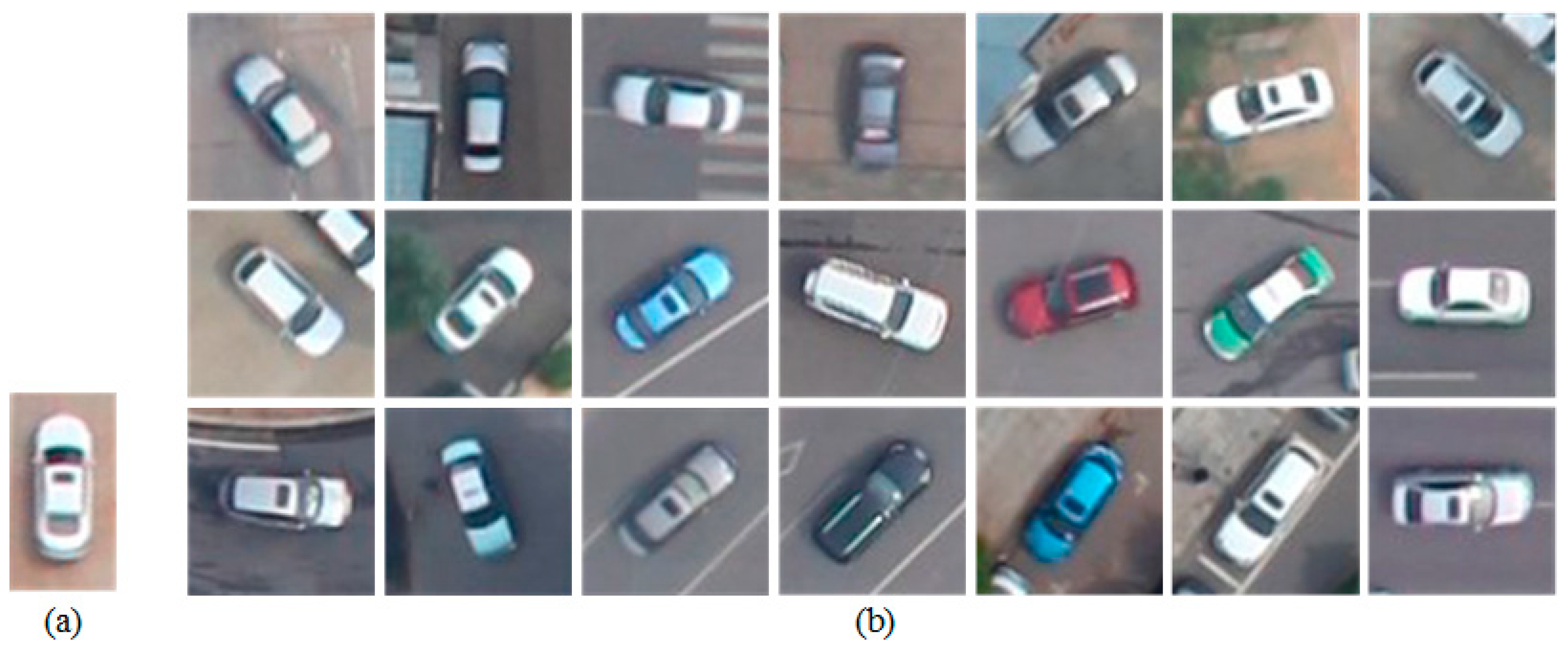
A detailed vehicle detection workflow is illustrated in Figure 1. As shown in Figure 1, for a test image, we first over-segment it into a group of superpixels using the simple linear iterative clustering (SLIC) superpixel segmentation method [54]. Then, centered at each superpixel, a patch is generated with a size of $n_{\mathrm{p}}\times n_{\mathrm{p}}$ pixels. Then, to estimate the existence of vehicles from these patches, we proposed an affine-function transformation-based object matching method, in which both the template and each of the patches, a collection of scale-invariant feature transform (SIFT) feature points are generated and characterized with SIFT feature vectors, and then a vehicle template is selected for conducting matching between the template and each of the generated patches. Compared to traditional methods that usually adopt a sliding window strategy to generate a group of candidate regions for individual vehicle detection [8], we, in this paper, the SLIC superpixel segmentation method to generate meaningful and non-redundant patches as operating units for individual vehicle detection. The SLIC superpixel segmentation method is detailed in the literature [55]. In the following subsections, we focus on the description of the affine-function transformation-based object matching framework, followed by an optimal matching processing by using a successive convexification scheme in Section 2.2.

2.1. Affine-Function Transformation Based Object Matching

The problem of object matching can be defined as matching a group of template feature points, representing a specific object of interest, to another group of scene feature points, representing a scene containing an instance of the object of interest (See Figure 2). Each feature point has a unique location and is depicted with a feature vector that characterizes the local appearance around that location. The matched scene feature points should preserve similar local features and relative spatial relationships of the template feature points. Most of existing object matching techniques dedicate to seek for point-to-point matching results, which might show low performance when dealing with occlusions. In contrast, we propose an affine-function transformation-based object matching framework, whose objective is to determine each template feature point’s optimal transformation parameters (not point-to-point matching) so that the matching location (which may not be a specific scene feature point) of each template feature point is close to a scene feature point with similar local appearance and geometric structure.

(1) Affine-function transformation

Denote $n_{\mathrm{t}}$ and $n_{\mathrm{s}}$ as the numbers of template feature points and scene feature points, respectively. Let $P=\{{\mathit{p}}_i={[x_{{\mathit{p}}_i},y_{{\mathit{p}}_i}]}^{\mathrm{T}}|i=1,2,\dots ,n_{\mathrm{t}}\}$ and $Q=\{{\mathit{q}}_j={[x_{{\mathit{q}}_j},y_{{\mathit{q}}_j}]}^{\mathrm{T}}|j=1,2,\dots ,n_{\mathrm{s}}\}$ be the sets of template feature points and scene feature points, respectively. Then, our object matching objective is to optimize the transformation parameters of each template feature point in P based on the scene feature points in Q. Define $T_i({\Phi }_i):R^n\to R^2,i=1,2,\dots ,n_{\mathrm{t}}$ as an affine transformation function that transforms the ith template feature point ${\mathit{p}}_i$ into a location in the scene with transformation parameters ${\Phi }_i\in R^n$. The result of $T_i({\Phi }_i)$ is the corresponding matching location of template feature point ${\mathit{p}}_i$ in the scene. In this paper, we define the affine transformation function as follows:

$$T_i({\Phi }_i)=\left[\begin{array}{c}\begin{array}{ccc}\alpha & \beta & \varphi \end{array}\\ \begin{array}{ccc}\gamma & \delta & \phi \end{array}\end{array}\right]\left[\begin{array}{c}{x}_{p_i}\\ y_{p_i}\\ 1\end{array}\right]+\left[\begin{array}{c}{\xi }_i\\ {\vartheta }_i\end{array}\right]$$

(1)

where $T_i({\Phi }_i):R^8\to R^2$ computes the matching location of template feature point ${\mathit{p}}_i$ under an affine transformation with parameters ${\Phi }_i={\left[\alpha ,\beta ,\gamma ,\delta ,\varphi ,\phi ,{\xi }_i,{\vartheta }_i\right]}^{\mathrm{T}}\in R^8$. We define a separate affine transformation function for each template feature point. The matching location of a template feature point ${\mathit{p}}_i$ is computed by its corresponding function $T_i({\Phi }_i)$. In Equation (1), ${\left[\alpha ,\beta ,\gamma ,\delta ,\varphi ,\phi \right]}^{\mathrm{T}}$ are the global affine transformation parameters that are shared by all template feature points, whereas ${\left[{\xi }_i,{\vartheta }_i\right]}^{\mathrm{T}}$ are the local translation parameters for only template feature point ${\mathit{p}}_i$. Therefore, different template feature points might have different versions of ${\left[{\xi }_i,{\vartheta }_i\right]}^{\mathrm{T}}$. As illustrated in Figure 3, the local translation parameters allow small local deformations between the template feature points and their matched locations.

(2) Dissimilarity measure

According to the object matching principles, one objective is to match each template feature point ${\mathit{p}}_i$ to the corresponding location $T_i({\Phi }_i)$ in the scene with the constraint that the local appearances of ${\mathit{p}}_i$ and $T_i({\Phi }_i)$ should be similar. Therefore, we define a dissimilarity measure function $dis{s}_i(q):R^2\to R^1,i=1,2,\dots ,n_{\mathrm{t}}$, respectively, for each template feature point to measure the local appearance dissimilarities between template feature point ${\mathit{p}}_i$ and its corresponding matched location q in the scene. Generally, two feature points having similar local appearances will result in a low dissimilarity measure value.

To solve the object matching problem, our overall objective is to determine the optimal transformation parameters ${\Phi }_1,{\Phi }_2,\dots ,{\Phi }_{n_{\mathrm{t}}}$ for template feature points ${\mathit{p}}_1,{\mathit{p}}_2,\dots ,{\mathit{p}}_{n_{\mathrm{t}}}$ to minimize the following objective function:

$$\begin{array}{l}\underset{{\Phi }_1,{\Phi }_2,\dots ,{\Phi }_{n_{\mathrm{t}}}}{\mathrm{minimize}}{\displaystyle \sum _{i=1}^{n_{\mathrm{t}}}dis{s}_i(T_i({\Phi }_i))}+R\left({\Phi }_1,{\Phi }_2,\dots ,{\Phi }_{n_{\mathrm{t}}}\right),\\ \mathrm{subject}\mathrm{to}{C}_j\left({\Phi }_1,{\Phi }_2,\dots ,{\Phi }_{n_{\mathrm{t}}}\right)\le 0,j=1,2,\dots ,n_{\mathrm{c}}\end{array}$$

(2)

where $dis{s}_i(T_i({\Phi }_i))$ computes the local appearance dissimilarity between template feature point ${\mathit{p}}_i$ and its corresponding matching location $T_i({\Phi }_i)$ in the scene. $R\left({\Phi }_1,{\Phi }_2,\dots ,{\Phi }_{n_{\mathrm{t}}}\right)$ denotes a convex relaxation term regularizing the transformation parameters. $C_j\left({\Phi }_1,{\Phi }_2,\dots ,{\Phi }_{n_{\mathrm{t}}}\right)\le 0,j=1,2,\dots ,n_{\mathrm{c}}$ defines a series of convex constraints. Here, $n_{\mathrm{c}}$ is the number of convex constraints. By such a definition, the overall objective function in Equation (2) can be effectively solved through convex optimization techniques. Next, we focus on the design of the dissimilarity measure function.

Recall that each feature point is associated with a location, as well as a feature vector characterizing the local appearance around that location. In this paper, each feature point is described using a scale-invariant feature transform (SIFT) vector [56]. Let $Cos{t}_{i,j},i=1,2,\dots ,n_{\mathrm{t}},j=1,2,\dots ,n_{\mathrm{s}}$ denote the feature dissimilarity between a template feature point ${\mathit{p}}_i$ and a scene feature point ${\mathit{q}}_j$. Then, we define $Cos{t}_{i,j}$ as the square root of the ${\mathsf{\chi }}^2$ distance [57] between the SIFT feature vectors of ${\mathit{p}}_i$ and ${\mathit{q}}_j$ as follows:

$$Cos{t}_{i,j}=\sqrt{{\displaystyle {\sum }_k\frac{{\left({\mathit{F}}_{{\mathit{p}}_i}^k-{\mathit{F}}_{{\mathit{q}}_j}^k\right)}^2}{{\mathit{F}}_{{\mathit{p}}_i}^k+{\mathit{F}}_{{\mathit{q}}_j}^k}}}$$

(3)

where ${\mathit{F}}_{{\mathit{p}}_i}^k$ and ${\mathit{F}}_{{\mathit{q}}_j}^k$ are the kth channels of the SIFT feature vectors of feature points ${\mathit{p}}_i$ and ${\mathit{q}}_j$, respectively. Then, for each template feature point ${\mathit{p}}_i,i=1,2,\dots ,n_{\mathrm{t}}$, we define a discrete version of the dissimilarity measure function $Dis{s}_i({\mathit{q}}_j):Q\to R^1,i=1,2,\dots ,n_{\mathrm{t}}$ as follows:

$$Dis{s}_i({\mathit{q}}_j)=Cos{t}_{i,j},j=1,2,\dots ,n_{\mathrm{s}},{\mathit{q}}_j\in Q$$

(4)

The domain of this function indicates that a template feature point ${\mathit{p}}_i$ can be only matched to a certain scene feature point ${\mathit{q}}_j$ with the feature dissimilarity measure determined by function $Dis{s}_i({\mathit{q}}_j)$. Minimizing $Dis{s}_i({\mathit{q}}_j)$ still results in a point-to-point matching pattern, which violates our objective to optimize the affine transformation parameters to compute the matching locations. Moreover, the discrete function $Dis{s}_i({\mathit{q}}_j)$ is non-convex. Therefore, adopting $Dis{s}_i({\mathit{q}}_j)$ as the dissimilarity measure in Equation (2) to minimize the overall objective function is difficult and cannot effectively obtain optimal solutions.

(3) Convex dissimilarity measure

To solve the aforementioned problem, we relax each discrete function $Dis{s}_i({\mathit{q}}_j)$ and construct a continuous and convex dissimilarity measure function $dis{s}_i(q)$, which can be effectively optimized through convex optimization techniques. To this end, for each template feature point ${\mathit{p}}_i,i=1,2,\dots ,n_{\mathrm{t}}$, we organize all the scene feature points together with their feature dissimilarities $Cos{t}_{i,j},j=1,2,\dots ,n_{\mathrm{s}}$ as a set of three-dimensional (3D) points $\{{[x_{{\mathit{q}}_j},y_{{\mathit{q}}_j},Cos{t}_{i,j}]}^{\mathrm{T}}|j=1,2,\dots ,n_{\mathrm{s}}\}$, whose first two dimensions are the location of a scene feature point and the third dimension is the corresponding feature dissimilarity. As illustrated in Figure 4, we give an example of the feature dissimilarities, viewed as a 3D point set, of the scene feature points associated with a template feature point. Obviously, this is actually the discrete version of the dissimilarity measure function $Dis{s}_i({\mathit{q}}_j)$.

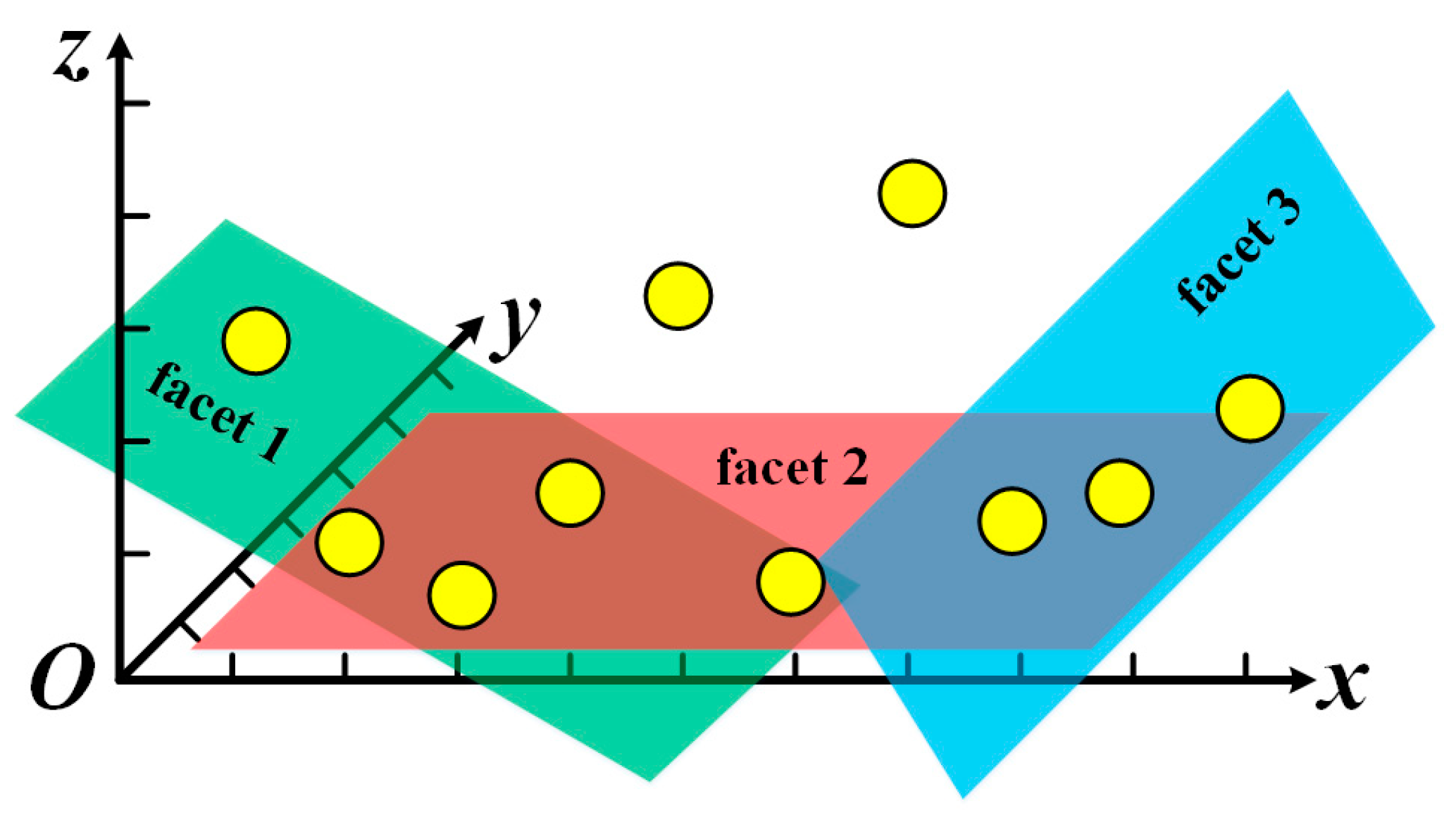
We construct the convex dissimilarity measure function $dis{s}_i(q)$ based on the lower convex hull of the 3D point set associated with template feature point ${\mathit{p}}_i$ with respect to the feature dissimilarity dimension. As shown in Figure 3, the facets are the lower convex hull of the 3D point set. Denote $\{z=a_{k}x+b_{k}y+c_k|k=1,2,\dots ,n_{\mathrm{f}}\}$ as the plane functions defining the $n_{\mathrm{f}}$ facets on the lower convex hull. ${\left[a_k,b_k,c_k\right]}^{\mathrm{T}}$ are the plane parameters of the kth plane. Then, we define the continuous convex dissimilarity measure function as follows:

$$dis{s}_i\left({[x,y]}^{\mathrm{T}}\right)=\underset{k}{\max }\left(a_{k}x+b_{k}y+c_k\right),k=1,2,\dots ,n_{\mathrm{f}}$$

(5)

where ${[x,y]}^{\mathrm{T}}$ can be any location in the scene domain. In other words, by such a relaxation, template feature point ${\mathit{p}}_i$ can be matched to any location ${[x,y]}^{\mathrm{T}}$ in the scene, not necessarily being a specific scene feature point. To effectively minimize Equation (5), we convert it into an equivalent linear programming problem:

$$\begin{array}{ll}\underset{x,y}{\mathrm{minimize}}dis{s}_i\left({[x,y]}^{\mathrm{T}}\right)\iff & \underset{x,y,u_i}{\mathrm{minimize}}{u}_i\\ & \mathrm{subject}\mathrm{to}{a}_{k}x+b_{k}y+c_k\le u_i,k=1,2,\dots ,n_{\mathrm{f}}\end{array}$$

(6)

where $u_i$ is an auxiliary variable representing the upper bound of $dis{s}_i\left({[x,y]}^{\mathrm{T}}\right)$. Equation (6) can be efficiently optimized using convex optimization techniques.

In order to use Equation (6) to minimize $dis{s}_i(T_i({\Phi }_i))$ in the overall objective function in Equation (2), we rewrite the affine transformation function $T_i({\Phi }_i)$ into $T_i({\Phi }_i)={\left[f_i({\Phi }_i),g_i({\Phi }_i)\right]}^{\mathrm{T}}$, where $f_i({\Phi }_i)=\alpha x_{p_i}+\beta y_{p_i}+\varphi +{\xi }_i$ and $g_i({\Phi }_i)=\gamma x_{p_i}+\delta y_{p_i}+\phi +{\vartheta }_i$ are affine functions that computes the x and y components of the matching location of template feature point ${\mathit{p}}_i$. By substituting x and y in Equation (6) with $f_i({\Phi }_i)$ and $g_i({\Phi }_i)$, we obtain the following convex optimization model which is equivalent to minimizing $dis{s}_i(T_i({\Phi }_i))$ with respect to transformation parameters ${\Phi }_i$:

$$\begin{array}{ll}\underset{{\Phi }_i}{\mathrm{minimize}}dis{s}_i\left(T_i({\Phi }_i)\right)& \iff \underset{{\Phi }_i,u_i}{\mathrm{minimize}}{u}_i\\ & \mathrm{subject}\mathrm{to}{a}_k{f}_i({\Phi }_i)+b_k{g}_i({\Phi }_i)+c_k\le u_i,k=1,2,\dots ,n_{\mathrm{f}}\end{array}$$

(7)

Then, summing up all the minimization terms $dis{s}_i(T_i({\Phi }_i)),i=1,2,\dots ,n_{\mathrm{t}}$ results in our overall objective function with respect to optimizing the affine transformation parameters ${\Phi }_1,{\Phi }_2,\dots ,{\Phi }_{n_{\mathrm{t}}}$ with convex constraints defined in Equation (7):

$$\underset{{\Phi }_1,{\Phi }_2,\dots ,{\Phi }_{n_{\mathrm{t}}}}{\mathrm{minimize}}{\displaystyle \sum _{i=1}^{n_{\mathrm{t}}}dis{s}_i(T_i({\Phi }_i))}+\lambda {{\displaystyle \sum _{i=1}^{n_{\mathrm{t}}}\Vert \left[\begin{array}{c}{\xi }_i\\ {\vartheta }_i\end{array}\right]\Vert }}_2^2$$

(8)

where the regularization term functions to penalize local deformations of the matching locations in the scene. It indicates that the local deformations of the matching locations should not be too large. $\lambda$ is a parameter that weights the dissimilarity measure term and the regularization term.

When partial occlusions of an object of interest exist in the scene, directly optimizing Equation (8) may degrade the performance of the proposed affine-function transformation-based object matching framework. To solve this problem, we assign a weight factor $w_i,i=1,2,\dots ,n_{\mathrm{t}}$ for each template feature point ${\mathit{p}}_i$ to describe its distinctiveness and contribution to the matching. Then, we obtain the final overall objective function with convex constraints defined in Equation (7) as follows:

$$\underset{{\Phi }_1,{\Phi }_2,\dots ,{\Phi }_{n_{\mathrm{t}}}}{\mathrm{minimize}}{\displaystyle \sum _{i=1}^{n_{\mathrm{t}}}{w}_i\cdot dis{s}_i(T_i({\Phi }_i))}+\lambda {{\displaystyle \sum _{i=1}^{n_{\mathrm{t}}}\Vert \left[\begin{array}{c}{\xi }_i\\ {\vartheta }_i\end{array}\right]\Vert }}_2^2$$

(9)

2.2. Successive Convexification Scheme for Solving the Objective Function

Recall that the continuous convex dissimilarity measure function $dis{s}_i({[x,y]}^{\mathrm{T}}):R^2\to R^1$ is constructed by relaxing the discrete dissimilarity measure function $Dis{s}_i(q):Q\to R^1$ based on the lower convex hull. If the feature descriptions of feature points are distinctive, the dissimilarity measures, computed using $Dis{s}_i(q)$, between a template feature point and all the scene feature points differ significantly. Therefore, the lower convex hull relaxation provides a satisfactory lower bound to the discrete measure function $Dis{s}_i(q)$. However, when features are not distinctive, the lower convex hull might not generate a very tight lower bound to $Dis{s}_i(q)$. To solve this problem, we propose a successive convexification scheme, similar to that adopted by Jiang et al. [58], to iteratively optimize the overall objective function to obtain a tighter solution.

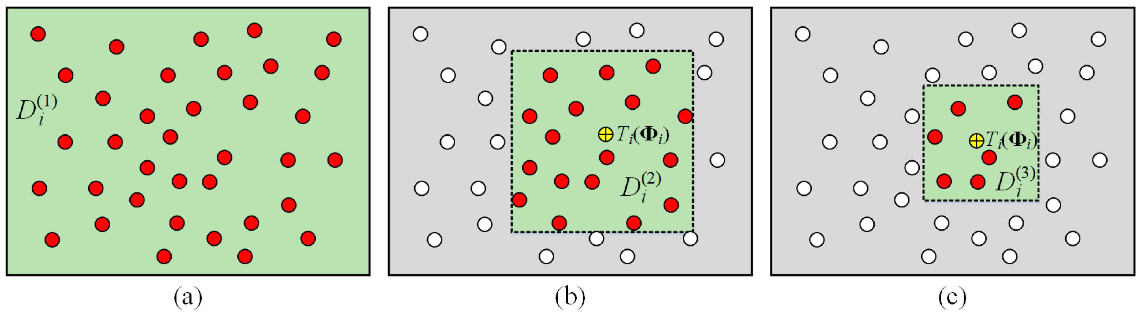
Initially, we assign an identical weight factor $w_i=1,i=1,2,\dots ,n_{\mathrm{t}}$ to all template feature points. In each iteration of the convexification, a trust region is defined for each template feature point. Only the scene feature points within the trust region can be used to construct the convex dissimilarity measure functions. In the first iteration, we fix the weight factors $w_i=1,i=1,2,\dots ,n_{\mathrm{t}}$ and define the entire scene as the trust region for each template feature point ${\mathit{p}}_i$, as illustrated by $D_i^{(1)}$ in Figure 5a. That is, initially, all scene feature points are used to construct the convex dissimilarity measure functions. Then, these convex dissimilarity measure functions are applied to the overall objective function in Equation (9) to optimize the affine transformation parameters ${\Phi }_1,{\Phi }_2,\dots ,{\Phi }_{n_{\mathrm{t}}}$. The corresponding matching locations of template feature points are computed by $T_1({\Phi }_1),T_2({\Phi }_2),\dots ,T_{n_{\mathrm{t}}}({\Phi }_{n_{\mathrm{t}}})$. Afterwards, we adjust the weight factors $w_i,i=1,2,\dots ,n_{\mathrm{t}}$ to deal with partial occlusions. If the dissimilarity measure value $dis{s}_i(T_i({\Phi }_i))$ between template feature point ${\mathit{p}}_i$ and its matching location $T_i({\Phi }_i)$ is high, $w_i$ is decreased by $\Delta w$ (i.e., $w_i=w_i-\Delta w$) to degrade the contribution of ${\mathit{p}}_i$. Otherwise, if the dissimilarity measure value is low, $w_i$ is increased by $\Delta w$ (i.e., $w_i=w_i+\Delta w$) to upgrade the contribution of ${\mathit{p}}_i$. In this way, the actual matching locations $T_i({\Phi }_i)$ occluded by other objects in the scene will be considered less to optimize the overall objective function.

In the second iteration, we fix the weight factors $w_i,i=1,2,\dots ,n_{\mathrm{t}}$ and define a shrunken trust region centered at the matching location $T_i({\Phi }_i)={\left[f_i({\Phi }_i),g_i({\Phi }_i)\right]}^{\mathrm{T}}$ for each template feature point ${\mathit{p}}_i$. Only the scene feature points located within the trust region are used to construct the convex dissimilarity measure functions (See Figure 5b). Mathematically, the trust region of ${\mathit{p}}_i$ in the second iteration is defined as follows:

$$D_i^{(2)}=\left\{{[x,y]}^{\mathrm{T}}\in R^2|f_i({\Phi }_i)-\frac{L^{(2)}}{2}\le x\le f_i({\Phi }_i)+\frac{L^{(2)}}{2},g_i({\Phi }_i)-\frac{L^{(2)}}{2}\le y\le g_i({\Phi }_i)+\frac{L^{(2)}}{2}\right\}$$

(10)

where $L^{(2)}=\min (H_{\mathrm{s}},W_{\mathrm{s}})/2$ is the side length of the trust region in the second iteration. Here, $H_{\mathrm{s}}$ and $W_{\mathrm{s}}$ are the height and width of the scene, respectively. Then, we apply the convex dissimilarity measure functions constructed using the scene feature points in trust regions $D_i^{(2)},i=1,2,\dots ,n_{\mathrm{t}}$ to optimize the overall objective function to obtain a set of tighter affine transformation parameters ${\Phi }_1,{\Phi }_2,\dots ,{\Phi }_{n_{\mathrm{t}}}$. The tighter matching locations are represented by $T_1({\Phi }_1),T_2({\Phi }_2),\dots ,T_{n_{\mathrm{t}}}({\Phi }_{n_{\mathrm{t}}})$. Afterwards, we adjust the weight factors $w_i,i=1,2,\dots ,n_{\mathrm{t}}$ using the same principle as described in the first iteration.

The same optimization operations are performed in the subsequent iterations with smaller and smaller trust regions that consider fewer and fewer scene feature points (See Figure 5c). Specifically, in the kth iteration, the trust region is defined as follows:

$$D_i^{(k)}=\left\{{[x,y]}^{\mathrm{T}}\in R^2|f_i({\Phi }_i)-\frac{L^{(k)}}{2}\le x\le f_i({\Phi }_i)+\frac{L^{(k)}}{2},g_i({\Phi }_i)-\frac{L^{(k)}}{2}\le y\le g_i({\Phi }_i)+\frac{L^{(k)}}{2}\right\}$$

(11)

where $L^{(k)}=L^{(k-1)}/2$ is the side length of the trust region in the kth iteration. Generally, four iterations are enough. Through the proposed successive convexification scheme, we can obtain a tighter matching result with satisfactory consideration of handling partial occlusions.

After optimizing the overall objective function in Equation (9) through the proposed successive convexification scheme, we obtain two results: a set of affine transformation parameters ${\Phi }_1,{\Phi }_2,\dots ,{\Phi }_{n_{\mathrm{t}}}$ and a matching cost (i.e., the value of the overall objective function). 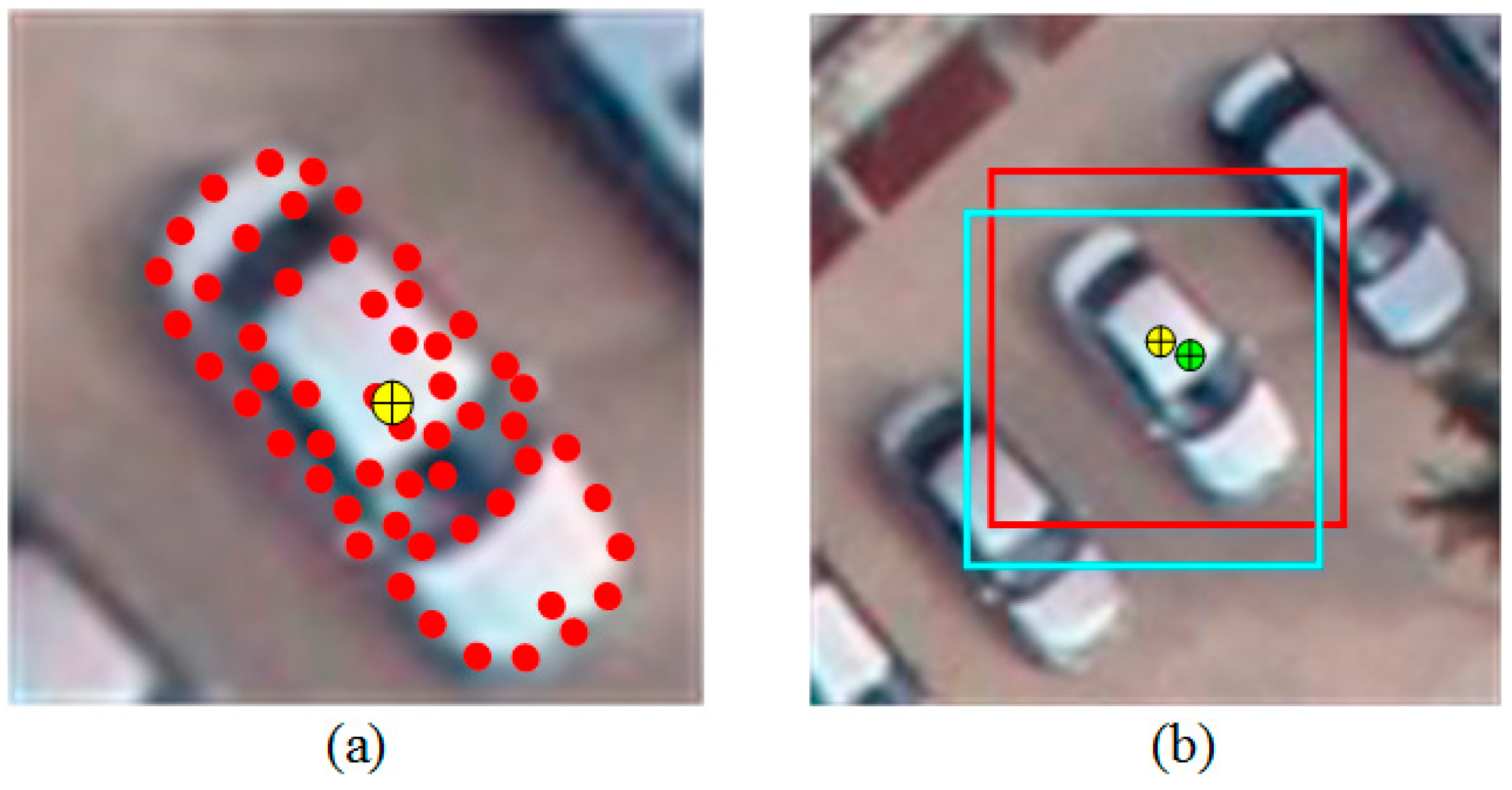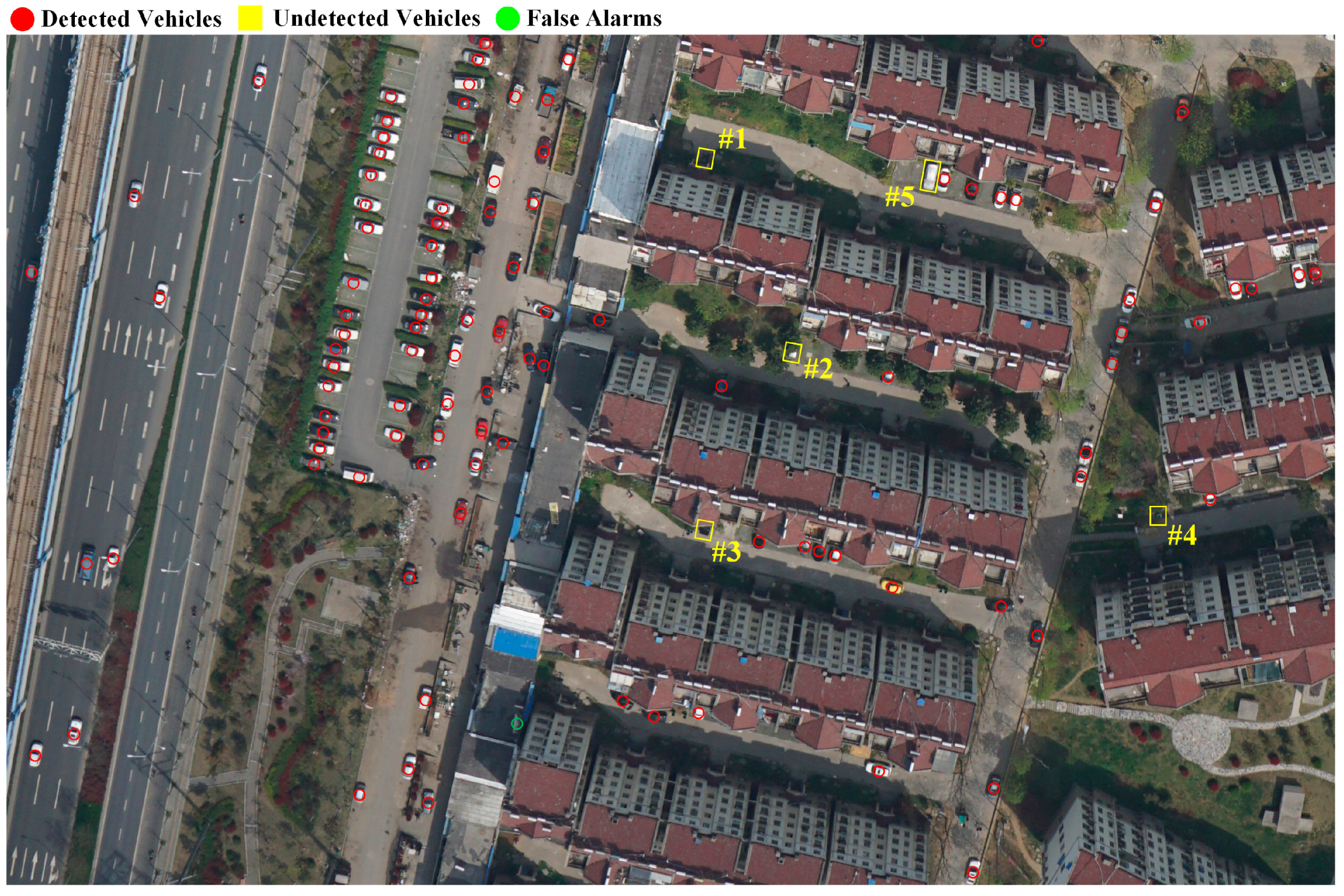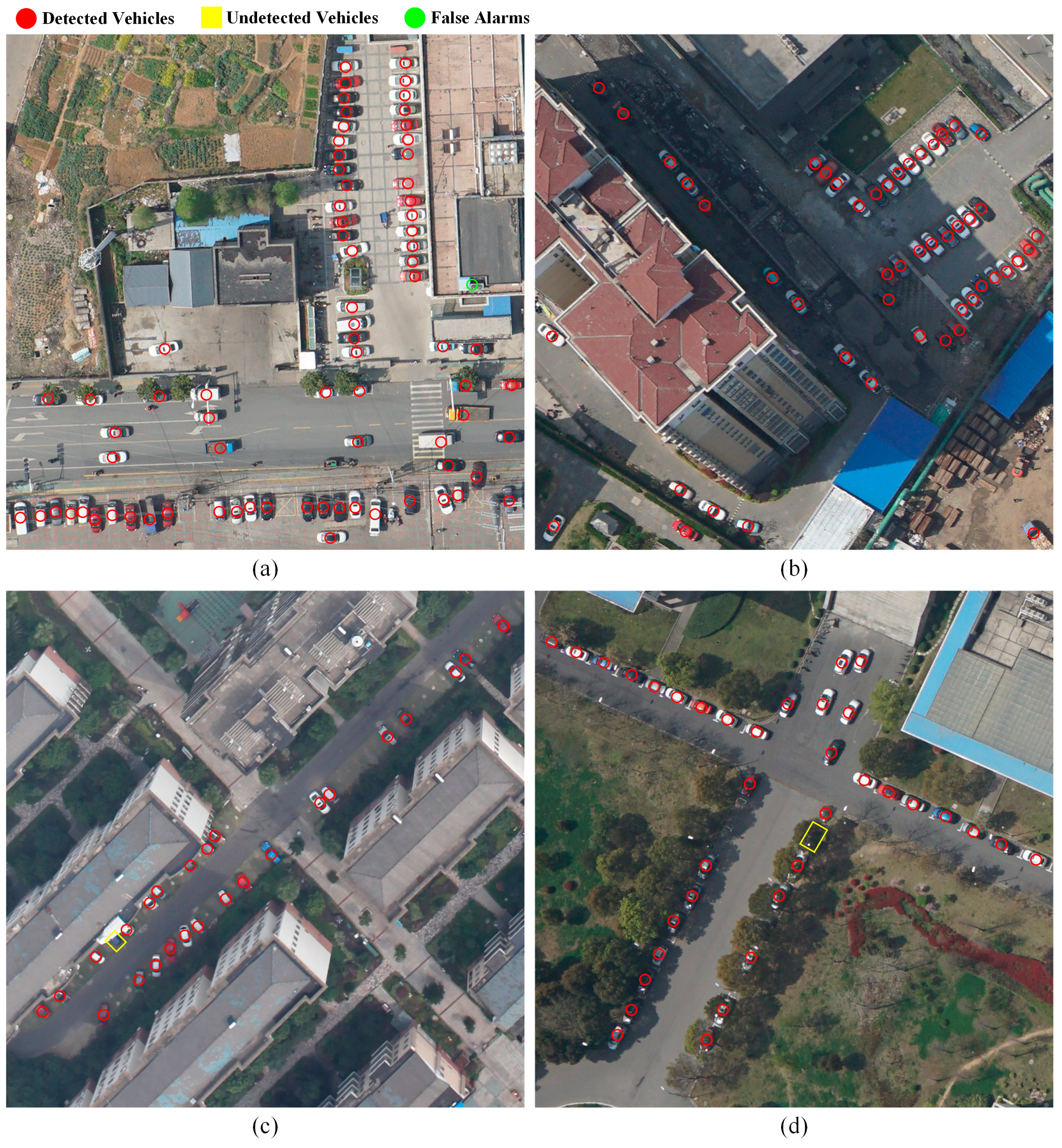The corresponding matching locations in the patch can be computed by $T_1({\Phi }_1),T_2({\Phi }_2),\dots ,T_{n_{\mathrm{t}}}({\Phi }_{n_{\mathrm{t}}})$, and the matching cost is used to estimate the existence of a vehicle in the patch. If the matching cost lies below a predefined threshold, we confirm that there is a vehicle instance in the patch. Then, as illustrated in Figure 6a, the location of the vehicle is estimated as the geometric centroid of the matching locations $T_1({\Phi }_1),T_2({\Phi }_2),\dots ,T_{n_{\mathrm{t}}}({\Phi }_{n_{\mathrm{t}}})$. However, as shown in Figure 6b, a vehicle instance might exist in multiple patches by using the superpixel segmentation-based patch generation strategy. Consequently, multiple locations are estimated for a single vehicle instance. In fact, these locations associated with a vehicle instance exhibit a cluster form and are extremely close to each other. Thus, we further adopt a non-maximum suppression process [55] to eliminate the repetitive detection results. The final vehicle detection result is illustrated in Figure 5.

3. Results and Discussions

3.1. Study Areas and Datasets

In this paper, we tested our proposed vehicle detection method on the UAV images. The UAV images used in this study were captured using the DJI Phantom 4 Pro UAV system (See Figure 7a). This is a quadrotor aircraft mounted with a one-inch high-resolution Exmor R CMOS image sensor. The maximum measuring frequency is 20 Hz. The detailed specification of the DJI Phantom 4 Pro UAV system is listed in

Table 1. Specification of the DJI Phantom 4 Pro Unmanned Aerial Vehicle (UAV) system.

Parameter	Value
Manufacturer	DJI
Weight	1388 g
Maximum horizontal flight speed	72 km/h
Maximum take-off altitude	6000 m
Maximum flight height	500 m
Maximum flight time	30 min
Maximum wind speed tolerable	10 m/s
Field of view	front-back: 70o, left-right: 50o
Measuring frequency	20 Hz
Image sensor	1 inch Exmor R CMOS sensor, 20M pixels
Image size	5472 × 3648 pixels
Maximum control distance	7000 m

. While surveying, we set the image capture mode to be “BURST mode” (a continuous shooting mode) with an image capture interval of 2 seconds. Therefore, a total number of 30 images with a size of 5472 × 3648 pixels were captured every minute.

In this study, two UAV image datasets were collected in two different urban areas for evaluating the proposed vehicle detection method. As shown in Figure 7b, the first dataset was collected in the urban area of City Nanjing, Jiangsu Province, China in 2016. The surveying area had a size of about 5.0 × 5.5 km². While surveying, the UAV system was flying at a height of about 150 m with a horizontal flight speed of about 15 m/s. A total number of 30,728 UAV images were collected to form the first dataset. As shown in Figure 7c, the second dataset was collected in the urban area of City Changsha, Hunan Province, China, in 2017. The surveying area had a size of about 7.5× 6.0 km². While surveying, the UAV system was flying at a height of about 150 m with a horizontal flight speed of about 16 m/s. A total number of 44,180 UAV images were captured to form the second dataset.

3.2. Robustness Evaluation

In the UAV images, different vehicles exhibit different sizes and orientations. Some are even partially occluded by other high-rise objects (e.g., trees and buildings). The illumination conditions and the vibrations of the surveying platform also affect the quality of the captured images. Thus, the proposed vehicle detection method should have the capability to effectively deal with the aforementioned circumstances. In this section, we evaluated the robustness of the proposed affine-function transformation-based object matching framework to scale variations, orientation variations, partial occlusions, and noise contaminations. To this end, we manually created a scene test dataset containing 500 scenes, each of which contains a vehicle instance. A subset of the test scene dataset is shown in Figure 8b. The same vehicle template shown in Figure 8a was used to conduct matching in all the experiments. For each matching experiment between the template and a scene, a group of feature points were extracted and described using the SIFT features. Then, we applied the affine-function transformation-based object matching framework to a pair of template and scene to conduct matching. After matching, if the matching cost was below a predefined threshold, the scene was regarded as correctly matched. Otherwise, it was regarded as a bad matching.

To examine the properties of the proposed object matching framework to scale variations, we transformed each scene with the following scale factors: 0.4, 0.5, 0.6, 0.8, 1.0, 1.2, 1.4, 1.5, 1.6, 1.8, and 2.0. Therefore, a scale variation test dataset containing 5500 scenes was created for robustness evaluation. Figure 9a shows an example of a scene transformed with different scales. Then, we applied the affine-function transformation-based object matching framework to the template shown in Figure 8a and each scene in the scale variation test dataset to conduct matching. The matching results are detailed in

Table 2. Vehicle matching results on the scale variation test dataset.

Scale	0.4	0.5	0.6	0.8	1.0	1.2	1.4	1.5	1.6	1.8	2.0
Matching rate	0.94	0.98	1.0	1.0	1.0	1.0	1.0	1.0	1.0	1.0	1.0

. We used the matching rate, which was defined as the proportion of correctly matched scenes, to analyze the matching performance in different scales. As shown in Table 2, when the scenes were enlarged by scale factors ranging from 1.2 to 2.0, as well as shrunk by scale factors 0.6 and 0.8, the matching performance was unaffected. This is because when a scene is enlarged or shrunk slightly, the features of the feature points and their relative position relationships are almost unchanged. Thus, the proposed matching framework obtained stable performance. However, when the scenes were shrunk by scale factors 0.4 and 0.5, some of the scenes were not correctly matched, resulting in a decrease of the matching rate. In fact, when a scene is shrunk greatly, the local descriptions of the feature points will change greatly. In addition, the distinctiveness between the feature points will diminish. Moreover, some adjacent feature points might be merged into one feature point. Thus, the matching performance was degraded. Fortunately, in actual UAV images captured with a bird view, the scale variations among vehicles are not very big, since the sizes of vehicles do not change dramatically. Therefore, the matching performance is hardly affected.

To test the robustness of the proposed object matching framework to rotation variations, we successively rotated each scene clockwise with an angle interval of 30 degrees. Therefore, a rotation variation test dataset including 6000 scenes was created for robustness evaluation. Figure 9b presents an example of a scene rotated with different angles. Then, object matching was carried out between the template and each of the rotated scenes. The vehicle matching results in different rotations are listed in

Table 3. Vehicle matching results on the rotation variation test dataset.

Rotation	0°	30°	60°	90°	120°	150°	180°	210°	240°	270°	300°	330°
Matching rate	1.0	1.0	1.0	1.0	1.0	1.0	1.0	1.0	1.0	1.0	1.0	1.0

. As reflected in Table 3, the matching rates were the same and unaffected by the rotations of scenes. This is because, when a scene is rotated, the features of the feature points, as well as their relative position relationships, still maintain without any modifications. Thus, the proposed matching framework performed equally under different rotation variations. This property is very useful for handling real world scenes, since vehicles always exhibit with different orientations.

To assess the performance of the proposed object matching framework to occlusion variations, we manually masked the vehicle instance in each scene with the following proportions of occlusions: 0%, 10%, 20%, 30%, 40%, 50%, 60%, 70%, 80%, and 90%. Therefore, an occlusion variation test dataset containing 5000 scenes was created for robustness evaluation. Figure 9c shows an example of a vehicle instance occluded with different proportions. Then, object matching was performed on each pair of the template and an occluded scene.

Table 4. Vehicle matching results on the occlusion variation test dataset.

Occlusion Proportion	0%	10%	20%	30%	40%	50%	60%	70%	80%	90%
Matching rate	1.0	1.0	1.0	1.0	1.0	0.98	0.82	0.51	0.32	0.17

details the vehicle matching results. As shown in Table 4, when the vehicles were partially occluded slightly (occlusion proportions ranging from 10% to 40%), the proposed matching framework performed effectively. All the scenes were correctly matched. This is benefited from the introduction of the weight factors in the overall objective function for evaluating the contributions of different feature points to a matching. When half part of a vehicle instance was occluded, the matching performance was slightly affected but still satisfactory. However, when the vehicle instances were occluded significantly, the matching performance dramatically decreased. This is because, when a vehicle instance is occluded significantly, the number of feature points contributing to the matching become very less. The majority of the matching locations computed through the affine transformation parameters are not correct, resulting in high dissimilarity measure values.

To evaluate the robustness of the proposed object matching framework to noises, we superimposed each scene with different levels of “salt and pepper” noises. We tested the following noise densities in our experiments: 0.00, 0.02, 0.05, 0.08, 0.10, 0.12, 0.15, 0.18, 0.20, 0.22, 0.25, 0.28, and 0.30. Therefore, a noise contamination dataset including 6500 scenes was constructed for robustness evaluation. Then, we applied the proposed object matching framework to the template and each of the noise-contaminated scenes to conduct matching.

Table 5. Vehicle matching results on the noise contamination dataset.

Noise Density	0.00	0.02	0.05	0.08	0.10	0.12	0.15	0.18	0.20	0.22	0.25	0.28	0.30
Matching rate	1.0	1.0	1.0	1.0	1.0	1.0	1.0	1.0	0.97	0.93	0.88	0.81	0.78

presents the vehicle matching results analyzed using the matching rate. As reflected in Table 5, the proposed object matching framework showed superior performance when the scenes were contaminated with low densities of noises. This is benefitted from the robustness of the SIFT feature descriptor, which has excellent properties of noise resistance. However, when the scenes were contaminated with high levels of noises, the feature descriptions of the feature points would be influenced, resulting in feature difference between a template feature point and its matching location. Thus, the dissimilarity measures between the template feature points and their matching locations became higher.

3.3. Vehicle Detection

To evaluate the performance of our proposed vehicle detection method, we applied it to the Nanjing and Changsha UAV image datasets aforementioned in Section 3.1. For a test image, first, we over-segmented it into a series of superpixels using the SLIC superpixel segmentation method. Then, meaningful and non-redundant patches were generated centered at each superpixel. In the UAV images, the length of a vehicle is approximately 54 pixels. Thus, in order to enclose an entire vehicle instance in a patch with some relaxations, we set the patch size to be 70 × 70 pixels. Next, object matching between the vehicle template shown in Figure 8a and each of the generated patches was carried out using the proposed affine-function transformation-based object matching framework. To successively optimize the overall objective function to obtain a group of tight transformation parameters, we performed four iterations of the successive convexification process and configured the weight adjustment factor as $\Delta w=0.2$. After matching cost thresholding, vehicle location estimation, and multiple detection results elimination, we obtained the final vehicle detection result.

Table 6. Vehicle detection results and quantitative evaluations on the Nanjing and Changsha Unmanned Aerial Vehicle (UAV) image datasets.

Dataset	Ground Truth	Detection Results		Quantitative Evaluations
		Vehicles	False Alarms	Completeness	Correctness	Quality	F1-Measure
Nanjing	672,184	613,032	17,659	0.912	0.972	0.889	0.941
Changsha	896,722	813,327	28,626	0.907	0.966	0.879	0.936
Average	1568,906	1426,359	46,285	0.909	0.969	0.883	0.938

lists the vehicle detection results, as well as the ground truths, on the two UAV image datasets. As reflected in Table 6, for each of the datasets, the majority of vehicles were correctly detected and only a small number of false alarms were generated. However, the number of false alarms took a very small proportion and was acceptable. For visual inspections, Figure 10 and Figure 11 illustrate a subset of the vehicle detection results on the two UAV image datasets. As shown in these figures, the vehicles exhibiting with different colors, different sizes, different orientations, different illumination conditions, different densities, and different levels of occlusions were effectively detected by the proposed vehicle detection method. Specifically, as shown in Figure 11a, for a scene with very high density of vehicles, the proposed method still obtained promising vehicle detection results. Figure 11b shows a scene containing vehicles covered with large areas of shadows. These shadows might affect the appearance and the saliency of the vehicles. Fortunately, benefiting from the use of the SIFT features, which has a strong property of invariance to illumination variations, these vehicles were correctly detected by using the proposed method. However, as shown by the vehicle marked by a yellow box labeled with #1 in Figure 10, it was covered with a severe shadow. The vehicle was almost hidden in the background. Thus, our proposed method failed to detect it because of extremely low distinctiveness of feature points. As shown in Figure 11c,d, some vehicles were partially occluded by high-rise buildings and overhead trees. Since in our proposed affine-function transformation-based object matching framework, occlusion is considered and handled by assigning each template feature point with a weight factor, which is successively adjusted to degrade the contributions of occluded matching positions in the successive convexification process. Therefore, our proposed method still achieved promising performance on such occluded vehicles. However, as shown by the vehicles marked by yellow boxes labeled with #2, #3, and #4 in Figure 10 and the vehicles marked by yellow boxes in Figure 11c,d, these vehicles were occluded severely, resulting in very high matching costs. Therefore, they were failed to be detected. In addition, as shown by the vehicle marked by a yellow box labeled with #5, it was entirely covered with a cloth. Its appearance feature being a vehicle almost disappeared. Thus, it was also undetected. Moreover, due to the high similarities of some real-world objects (e.g., air conditioner external units) to the vehicles, they were falsely detected as vehicles caused by low matching costs.

To quantitatively evaluate the accuracy and correctness of the vehicle detection results on the two UAV image datasets, we adopted the following four quantitative measures: completeness, correctness, quality, and F1-measure [41]. Completeness assesses the proportion of correctly detected vehicles with respect to the ground truth. Correctness evaluates the proportion of correctly detected vehicles with respect to all the detected instances. Quality and F1-measure reflect the overall performance. They are defined as follows:

$$completeness=\frac{TP}{TP+FN}$$

(12)

$$correctness=\frac{TP}{TP+FP}$$

(13)

$$quality=\frac{TP}{TP+FN+FP}$$

(14)

$$F_1-measure=\frac{2\cdot completeness\cdot correctness}{completeness+correctness}$$

(15)

where TP, FN, and FP are the numbers of correctly detected vehicles, undetected vehicles, and falsely detected non-vehicle objects, respectively. The quantitative evaluation results using these four measures are listed in Table 6. The proposed vehicle detection method achieved a completeness, correctness, quality, and F1-measure of 0.912, 0.972, 0.889, and 0.941, respectively, on the Nanjing UAV image dataset. For the Changsha UAV image dataset, a completeness, correctness, quality, and F1-measure of 0.907, 0.966, 0.879, and 0.936, respectively, were obtained. On the whole, through visual inspections and quantitative evaluations, we confirmed that the proposed vehicle detection method performed effectively and was feasible for vehicle detection from UAV images.

The proposed vehicle detection method was tested on a cloud computing platform with eight 16-GB GPUs, one 16-core CPU, and a memory size of 64 GB. In practice, for a test image, after patch generation, the generated patches were distributed to the eight GPUs for parallel processing. The processing time of the proposed method was also recorded to analyze its computational performance. On average, the proposed method achieved a processing speed of 31 patches per second on a GPU. Thus, by adopting the parallel processing strategy, 248 patches were under processing every second.

3.4. Comparative Studies

To further compare the performance of the proposed method in this paper and other existing vehicle detection methods, a set of comparative experiments were conducted with the following nine existing vehicle detection methods: coupled region-based convolutional neural networks (CR-CNN) [49], hard example mining based convolutional neural networks (HEM-CNN) [23], affine invariant description and large-margin dimensionality reduction based method (AID-LDR) [17], bag-of-words and orientation aware scanning based method (BoW-OAS) [8], Viola-Jones based method (VJ) [18], enhanced Viola-Jones based method (EVJ) [19], fast binary detector based method (FBD) [21], YOLOv3 [59], and Faster R-CNN [36]. In the CR-CNN method, first, vehicle candidate regions are extracted based on a vehicle proposal network; then, a coupled region-based CNN is performed on the candidate regions to detect vehicles. For the HEM-CNN method, to train an effective CNN model, hard example mining is applied to the stochastic gradient descent to select informative training samples; then, the CNN model is used for vehicle detection based on a sliding window strategy. Both of the AID-LDR and BoW-OAS methods adopt the bag-of-words model to represent the statistical feature of a vehicle. The detection of vehicles is achieved through a sliding window-based classification process. For the VJ and EVJ methods, Viola–Jones object detection scheme is proposed to detect vehicles. To well handle vehicles of varying orientations, a road orientation adjustment method is adopted to make sure that roads and on-road vehicles are aligned with the horizontal direction. In the FBD method, a fast binary detector using integral channel features is designed to detect vehicles. YOLOv3 is a one-stage object detection network which accomplishes feature extraction and object prediction in a single network. In contrast, Faster R-CNN is a two-stage object detection framework composed of a region proposal network and an object detection network. The region proposal network generates a group of object proposals, which are further identified by the object detection network to verify the objects of interest.

We applied these nine methods to the Nanjing and Changsha UAV image datasets to evaluate their performances on vehicle detection. Quantitative evaluations using completeness, correctness, quality, and F1-measure were also carried out on the detection results. The detailed detection results and quantitative evaluations of different methods are listed in

Table 7. Vehicle detection results and quantitative evaluations of different methods.

Method	Dataset	Detection Results		Quantitative Evaluations
		Vehicles	False Alarms	Completeness	Correctness	Quality	F1-Measure
CR-CNN	Nanjing	564,635	32,231	0.840	0.946	0.802	0.890
	Changsha	752,350	54,027	0.839	0.933	0.791	0.884
HEM-CNN	Nanjing	545,142	32,951	0.811	0.943	0.773	0.872
	Changsha	719,172	49,996	0.802	0.935	0.760	0.863
AID-LDR	Nanjing	576,062	48,734	0.857	0.922	0.799	0.888
	Changsha	739,796	71,383	0.825	0.912	0.764	0.866
BoW-OAS	Nanjing	602,277	48,833	0.896	0.925	0.835	0.910
	Changsha	782,839	70,856	0.873	0.917	0.809	0.894
VJ	Nanjing	576,734	40,094	0.858	0.935	0.810	0.895
	Changsha	745,176	57,815	0.831	0.928	0.781	0.877
EVJ	Nanjing	590,850	35,050	0.879	0.944	0.835	0.910
	Changsha	772,078	56,332	0.861	0.932	0.810	0.895
FBD	Nanjing	580,767	41,706	0.864	0.933	0.814	0.897
	Changsha	759,524	66,944	0.847	0.919	0.788	0.882
YOLOv3	Nanjing	605,638	20,021	0.901	0.968	0.875	0.933
	Changsha	806,153	36,222	0.899	0.957	0.864	0.927
Faster R-CNN	Nanjing	612,360	16,993	0.911	0.973	0.889	0.941
	Changsha	811,533	27,695	0.905	0.967	0.878	0.935

. As reflected by the overall evaluations of quality and F1-measure, the HEM-CNN and AID-LDR methods obtained relatively lower performances on the two datasets; whereas the YOLOv3 and Faster R-CNN methods obtained the best performance. In addition, the BoW-OAS and EVJ methods obtained similar performances. By analyzing the number of correctly detected vehicles with respect to the ground truth and the number of correctly detected vehicles with respect to the detected objects, the YOLOv3 and Faster R-CNN methods outperformed the other seven methods with higher completeness and correctness values. This is because, these two methods adopt deep learning techniques to exploit high-level features of vehicles. Thus, they showed superior performance than the other methods. Comparatively, by using region proposal mechanism, Faster R-CNN performed a little better than YOLOv3. However, the AID-LDR and BoW-OAS methods generated more false alarms, thereby resulting in relatively lower correctness values than the other methods. This is because the AID-LDR and BoW-OAS methods adopt mid-level statistical features of vehicles represented using the bag-of-words model. According to the statistical property, the bag-of-words representation can only characterize the existence of some features; however, the relative relationships of these features cannot be reflected. As shown in Figure 12, Figure 12a is a patch containing a normal vehicle; Figure 12b and c are generated by cutting Figure 12a into four parts and making some transformations and combinations on these parts. Apparently, Figure 12b and c cannot be considered as a vehicle. However, the bag-of-words representations of these three patches are almost similar. They are equally detected as normal vehicles. Therefore, more false alarms were detected by the AID-LDR and BoW-OAS methods. Compared with these nine methods, our proposed method obtained compatible performance with the Faster R-CNN and outperformed the other eight methods. Through comparative studies, our proposed method can effectively tackle various scene conditions and obtained advantageous performance in accurately detecting vehicles from UAV images.

4. Conclusions

In this paper, we have proposed an affine-function transformation-based object matching framework for detecting vehicles from UAV images. The proposed method has advantageous properties to tackle scale variations, orientation variations, illumination variations, and partial occlusions of vehicles. For a test image, to generate meaningful and non-redundant patches, an SLIC-based superpixel segmentation strategy is adopted for patch generation. Then, the affine-function transformation-based object matching framework is applied to a vehicle template and each of the generated patches for vehicle existence estimation. Finally, after matching cost thresholding, vehicle location estimation, and multiple response elimination, vehicles are accurately detected and located in the image. The proposed method has been tested on two UAV image datasets for performance evaluation on vehicle detection. Quantitative evaluations confirmed that an average completeness, correctness, quality, and F1-measure of 0.909, 0.969, 0.883, and 0.938, respectively, were achieved towards vehicle detection. Visual inspections also showed the robustness of the proposed method in handling various vehicle conditions. In addition, comparative studies with nine existing vehicle detection methods demonstrated that the proposed method obtained compatible performance with the Faster R-CNN and outperformed the other eight methods in detecting vehicles from UAV images.

References

1. Liu, W.; Yamazaki, F.; Vu, T.T. Automated vehicle extraction and speed determination from QuickBird satellite images. IEEE J. Sel. Top. Appl. Earth Obs. Remote Sens. 2011, 4, 75–82. [Google Scholar] [CrossRef]
2. Zhou, H.; Kong, H.; Wei, L.; Creighton, D.; Nahavandi, S. On detecting road regions in a single UAV image. IEEE Trans. Intell. Transp. Syst. 2017, 18, 1713–1722. [Google Scholar] [CrossRef]
3. Li, M.; Stein, A.; Bijker, W.; Zhan, Q. Region-based urban road extraction from VHR satellite images using binary partition tree. Int. J. Appl. Earth Obs. Geoinf. 2016, 44, 217–225. [Google Scholar] [CrossRef]
4. Mokhtarzade, M.; Zoej, V.M.J. Road detection from high-resolution satellite images using artificial neural networks. Int. J. Appl. Earth Obs. Geoinf. 2007, 9, 32–40. [Google Scholar] [CrossRef] [Green Version]
5. Jin, H.; Feng, Y. Automated road pavement marking detection from high resolution aerial images based on multi-resolution image analysis and anisotropic Gaussian filtering. In Proceedings of the 2010 2nd International Conference on Signal Processing Systems, Dalian, China, 5–7 July 2010; pp. 337–341. [Google Scholar]
6. Pan, Y.; Zhang, X.; Cervone, G.; Yang, L. Detection of asphalt pavement potholes and cracks based on the unmanned aerial vehicle multispectral imagery. IEEE J. Sel. Top. Appl. Earth Obs. Remote Sens. 2018, 11, 3701–3712. [Google Scholar] [CrossRef]
7. Cao, L.; Luo, F.; Chen, L.; Sheng, Y.; Wang, H.; Wang, C.; Ji, R. Weakly supervised vehicle detection in satellite images via multi-instance discriminative learning. Pattern Recognit. 2017, 64, 417–424. [Google Scholar] [CrossRef]
8. Zhou, H.; Wei, L.; Lim, C.P.; Creighton, D.; Nahavandi, S. Robust vehicle detection in aerial images using bag-of-words and orientation aware scanning. IEEE Trans. Geosci. Remote Sens. 2018, 56, 7074–7085. [Google Scholar] [CrossRef]
9. Eslami, M.; Faez, K. Automatic traffic monitoring using satellite images. In Proceedings of the 2010 2nd International Conference on Computer Engineering and Technology, Chengdu, China, 16–18 April 2010; pp. 130–135. [Google Scholar]
10. Khalil, M.; Li, J.; Sharif, A.; Khan, J. Traffic congestion detection by use of satellites view. In Proceedings of the 2017 14th International Computer Conference on Wavelet Active Media Technology and Information Processing (ICCWAMTIP), Chengdu, China, 15–17 December 2017; pp. 278–280. [Google Scholar]
11. Kembhavi, A.; Harwood, D.; Davis, L.S. Vehicle detection using partial least squares. IEEE Trans. Pattern Anal. Mach. Intell. 2011, 33, 1250–1265. [Google Scholar] [CrossRef]
12. Zheng, Z.; Zhou, G.; Wang, Y.; Liu, Y.; Li, X.; Wang, X.; Jiang, L. A novel vehicle detection method with high resolution highway aerial image. IEEE J. Sel. Top. Appl. Earth Obs. Remote Sens. 2013, 6, 2338–2343. [Google Scholar] [CrossRef]
13. Chen, Z.; Wang, C.; Luo, H.; Wang, H.; Chen, Y.; Wen, C.; Yu, Y.; Cao, L.; Li, J. Vehicle detection in high-resolution aerial images based on fast sparse representation classification and multiorder feature. IEEE Trans. Intell. Transp. Syst. 2016, 17, 2296–2309. [Google Scholar] [CrossRef]
14. Holt, A.C.; Seto, E.Y.; Rivard, T.; Gong, P. Object-based detection and classification of vehicles from high-resolution aerial photography. Photogramm. Eng. Remote Sens. 2009, 75, 871–880. [Google Scholar] [CrossRef]
15. Niu, X. A semi-automatic framework for highway extraction and vehicle detection based on a geometric deformable model. ISPRS J. Photogramm. Remote Sens. 2006, 61, 170–186. [Google Scholar] [CrossRef]
16. Zhou, H.; Wei, L.; Creighton, D.; Nahavandi, S. Orientation aware vehicle detection in aerial images. Electron. Lett. 2017, 53, 1406–1408. [Google Scholar] [CrossRef]
17. Wan, L.; Zheng, L.; Huo, H.; Fang, T. Affine invariant description and large-margin dimensionality reduction for target detection in optical remote sensing images. IEEE Geosci. Remote Sens. Lett. 2017, 14, 1116–1120. [Google Scholar] [CrossRef]
18. Xu, Y.; Yu, G.; Wang, Y.; Wu, X.; Ma, Y. A hybrid vehicle detection method based on Viola-Jones and HOG+SVM from UAV images. Sensors 2016, 16, 1325. [Google Scholar] [CrossRef] [PubMed]
19. Xu, Y.; Yu, G.; Wu, X.; Wang, Y.; Ma, Y. An enhanced Viola-Jones vehicle detection method from unmanned aerial vehicles imagery. IEEE Trans. Intell. Transp. Syst. 2017, 18, 1845–1856. [Google Scholar] [CrossRef]
20. Audebert, N.; Saux, B.L.; Lefèvre, S. Segment-before-detect: Vehicle detection and classification through semantic segmentation of aerial images. Remote Sens. 2017, 9, 368. [Google Scholar] [CrossRef]
21. Liu, K.; Mattyus, G. Fast multiclass vehicle detection on aerial images. IEEE Geosci. Remote Sens. Lett. 2015, 12, 1938–1942. [Google Scholar]
22. Tuermer, S.; Kurz, F.; Reinartz, P.; Stilla, U. Airborne vehicle detection in dense urban areas using HOG features and disparity maps. IEEE J. Sel. Top. Appl. Earth Obs. Remote Sens. 2013, 6, 2327–2337. [Google Scholar] [CrossRef]
23. Koga, Y.; Miyazaki, H.; Shibasaki, R. A CNN-based method of vehicle detection from aerial images using hard example mining. Remote Sens. 2018, 10, 124. [Google Scholar] [CrossRef]
24. Moranduzzo, T.; Melgani, F. Detecting cars in UAV images with a catalog-based approach. IEEE Trans. Geosci. Remote Sens. 2013, 52, 6356–6367. [Google Scholar] [CrossRef]
25. Razakarivony, S.; Jurie, F. Vehicle detection in aerial imagery: A small target detection benchmark. J. Vis. Commun. Image Represent. 2016, 34, 187–203. [Google Scholar] [CrossRef]
26. Cao, L.; Jiang, Q.; Cheng, M.; Wang, C. Robust vehicle detection by combining deep features with exemplar classification. Neurocomputing 2016, 215, 225–231. [Google Scholar] [CrossRef]
27. Cao, L.; Wang, C.; Li, J. Vehicle detection from highway satellite images via transfer learning. Inf. Sci. 2016, 366, 177–187. [Google Scholar] [CrossRef]
28. Ammour, N.; Alhichri, H.; Bazi, Y.; Benjdira, B.; Alajlan, N.; Zuair, M. Deep learning approach for car detection in UAV imagery. Remote Sens. 2017, 9, 312. [Google Scholar] [CrossRef]
29. Chen, Z.; Wang, C.; Wen, C.; Teng, X.; Chen, Y.; Guan, H.; Luo, H.; Cao, L.; Li, J. Vehicle detection in high-resolution aerial images via sparse representation and superpixels. IEEE Trans. Geosci. Remote Sens. 2016, 54, 103–116. [Google Scholar] [CrossRef]
30. Zhang, J.; Tao, C.; Zou, Z. An on-road vehicle detection method for high-resolution aerial images based on local and global structure learning. IEEE Geosci. Remote Sens. Lett. 2017, 14, 1198–1202. [Google Scholar] [CrossRef]
31. Bazi, Y.; Melgani, F. Convolutional SVM networks for object detection in UAV imagery. IEEE Trans. Geosci. Remote Sens. 2018, 56, 3107–3118. [Google Scholar] [CrossRef]
32. Elmikaty, M.; Stathaki, T. Car detection in aerial images of dense urban areas. IEEE Trans. Aerosp. Electron. Syst. 2018, 54, 51–63. [Google Scholar] [CrossRef]
33. Liu, Y.; Monteiro, S.T.; Saber, E. Vehicle detection from aerial color imagery and airborne LiDAR data. In Proceedings of the 2016 IEEE International Geoscience and Remote Sensing Symposium (IGARSS), Beijing, China, 10–15 July 2016; pp. 1384–1387. [Google Scholar]
34. Schilling, H.; Bulatov, D.; Middelmann, W. Object-based detection of vehicles using combined optical and elevation data. ISPRS J. Photogramm. Remote Sens. 2018, 136, 85–105. [Google Scholar] [CrossRef]
35. Krizhevsky, A.; Sutskever, I.; Hinton, G.E. ImageNet classification with deep convolutional neural networks. In Proceedings of the Advances in Neural Information Processing Systems, Lake Tahoe, NV, USA, 3–6 December 2012; pp. 1097–1105. [Google Scholar]
36. Ren, S.; He, K.; Girshick, R.; Sun, J. Faster R-CNN: Towards real-time object detection with region proposal networks. IEEE Trans. Pattern Anal. Mach. Intell. 2017, 39, 1137–1149. [Google Scholar] [CrossRef] [PubMed]
37. Salakhutdinov, R.; Tenenbaum, J.B.; Torralba, A. Learning with hierarchical-deep models. IEEE Trans. Pattern Anal. Mach. Intell. 2013, 35, 1958–1971. [Google Scholar] [CrossRef] [PubMed]
38. Chen, G.; Zhang, X.; Wang, Q.; Dai, F.; Gong, Y.; Zhu, K. Symmetrical dense-shortcut deep fully convolutional networks for semantic segmentation of very-high-resolution remote sensing images. IEEE J. Sel. Top. Appl. Earth Obs. Remote Sens. 2018, 11, 1633–1644. [Google Scholar] [CrossRef]
39. Kemker, R.; Salvaggio, C.; Kanan, C. Algorithms for semantic segmentation of multispectral remote sensing imagery using deep learning. ISPRS J. Photogramm. Remote Sens. 2018, 145, 60–77. [Google Scholar] [CrossRef] [Green Version]
40. Ding, P.; Zhang, Y.; Deng, W.J.; Jia, P.; Kuijper, A. A light and faster regional convolutional neural network for object detection in optical remote sensing images. ISPRS J. Photogramm. Remote Sens. 2018, 141, 208–218. [Google Scholar] [CrossRef]
41. Yu, Y.; Guan, H.; Zai, D.; Ji, Z. Rotation-and-scale-invariant airplane detection in high-resolution satellite images based on deep-Hough-forests. ISPRS J. Photogramm. Remote Sens. 2016, 112, 50–64. [Google Scholar] [CrossRef]
42. Han, W.; Feng, R.; Wang, L.; Cheng, Y. A semi-supervised generative framework with deep learning features for high-resolution remote sensing image scene classification. ISPRS J. Photogramm. Remote Sens. 2018, 145, 23–43. [Google Scholar] [CrossRef]
43. Zhang, C.; Pan, X.; Li, H.; Gardiner, A.; Sargent, I.; Hare, J.; Atkinson, P.M. A hybrid MLP-CNN classifier for very fine resolution remotely sensed image classification. ISPRS J. Photogramm. Remote Sens. 2018, 140, 133–144. [Google Scholar] [CrossRef]
44. Wang, S.; Quan, D.; Liang, X.; Ning, M.; Guo, Y.; Jiao, L. A deep learning framework for remote sensing image registration. ISPRS J. Photogramm. Remote Sens. 2018, 145, 148–164. [Google Scholar] [CrossRef]
45. Sommer, L.; Schuchert, T.; Beyerer, J. Comprehensive analysis of deep learning based vehicle detection in aerial images. IEEE Trans. Circuits Syst. Video Tech. 2018, in press. [Google Scholar] [CrossRef]
46. Mou, L.; Zhu, X.X. Vehicle instance segmentation from aerial image and video using a multitask learning residual fully convolutional network. IEEE Trans. Geosci. Remote Sens. 2018, 56, 6699–6711. [Google Scholar] [CrossRef]
47. Wu, D.; Zhang, Y.; Chen, Y.; Zhong, S. Vehicle detection in high-resolution images using superpixel segmentation and CNN iteration strategy. IEEE Geosci. Remote Sens. Lett. 2019, 16, 105–109. [Google Scholar] [CrossRef]
48. Tang, T.; Zhou, S.; Deng, Z.; Zou, H.; Lei, L. Vehicle detection in aerial images based on region convolutional neural networks and hard negative example mining. Sensors 2017, 17, 336. [Google Scholar] [CrossRef]
49. Deng, Z.; Sun, H.; Zhou, S.; Zhao, J.; Zou, H. Toward fast and accurate vehicle detection in aerial images using coupled region-based convolutional neural networks. IEEE J. Sel. Top. Appl. Earth Obs. Remote Sens. 2017, 10, 3652–3664. [Google Scholar] [CrossRef]
50. Schilling, H.; Bulatov, D.; Niessner, R.; Middelmann, W.; Soergel, U. Detection of vehicles in multisensor data via multibranch convolutional neural networks. IEEE J. Sel. Top. Appl. Earth Obs. Remote Sens. 2018, 11, 4299–4316. [Google Scholar] [CrossRef]
51. Zhong, J.; Lei, T.; Yao, G. Robust vehicle detection in aerial images based on cascaded convolutional neural networks. Sensors 2017, 17, 2720. [Google Scholar] [CrossRef]
52. Yang, C.; Li, W.; Lin, Z. Vehicle object detection in remote sensing imagery based on multi-perspective convolutional neural network. ISPRS Int. J. Geo-Inf. 2018, 7, 249. [Google Scholar] [CrossRef]
53. Tang, T.; Zhou, S.; Deng, Z.; Lei, L.; Zou, H. Arbitrary-oriented vehicle detection in aerial imagery with single convolutional neural networks. Remote Sens. 2017, 9, 1170. [Google Scholar] [CrossRef]
54. Achanta, R.; Shaji, A.; Smith, K.; Lucchi, A.; Fua, P.; Süsstrunk, S. SLIC superpixels compared to state-of-the-art superpixel methods. IEEE Trans. Pattern Anal. Mach. Intell. 2012, 34, 2274–2282. [Google Scholar] [CrossRef]
55. Neubeck, A.; Van Gool, L. Efficient non-maximum suppression. In Proceedings of the 18th International Conference on Pattern Recognition (ICPR’06), Hong Kong, China, 20–24 August 2006; pp. 850–855. [Google Scholar]
56. Lowe, D.G. Distinctive image features from scale-invariant keypoints. Int. J. Comput. Vis. 2004, 60, 91–110. [Google Scholar] [CrossRef]
57. Wahl, E.; Hillenbrand, U.; Hirzinger, G. Surflet-pair-relation histograms: A statistical 3D-shape representation for rapid classification. In Proceedings of the Fourth International Conference on 3-D Digital Imaging and Modeling, 2003. 3DIM 2003, Banff, UK, 6–10 October 2003; pp. 474–481. [Google Scholar]
58. Jiang, H.; Drew, M.S.; Li, Z. Matching by linear programming and successive convexification. IEEE Trans. Pattern Anal. Mach. Intell. 2007, 29, 959–975. [Google Scholar] [CrossRef]
59. Redmon, J.; Farhadi, A. YOLOv3: An incremental improvement. arXiv 2018, arXiv:1804.02767v1. [Google Scholar]
Figure 1. Illustration of the vehicle detection workflow using the proposed affine-function transformation-based object matching framework.
Remotesensing 11 01708 g001
Figure 2. Illustration of object matching. (a) A group of template feature points representing a vehicle, (b) a group of scene feature points representing a scene containing a vehicle instance, and (c) the matched scene feature points.
Remotesensing 11 01708 g002
Figure 3. Illustration of the affine transformation model. q1 to q4 are, respectively, the corresponding matched locations of p1 to p4 after applying the affine transformation function.
Remotesensing 11 01708 g003
Figure 4. Illustration of the feature dissimilarity measures viewed as a 3D point set and the constructed convex dissimilarity measure function (facets).
Remotesensing 11 01708 g004
Figure 5. Illustration of the successive convexification scheme. (a) In the first iteration, all the scene feature points (red dots) are used to construct the convex dissimilarity measure function, (b) in the second iteration, only the scene feature points in the trust region (red dots) are used to construct the convex dissimilarity measure function, and (c) similar operations as those in the second iteration are performed in the latter iterations.
Remotesensing 11 01708 g005
Figure 6. Illustrations of (a) the vehicle location is estimated as the centroid of the matching locations (yellow dot), and (b) a vehicle existing in two patches generates two locations.
Remotesensing 11 01708 g006
Figure 7. Illustrations of (a) the DJI Phantom 4 Pro Unmanned Aerial Vehicle (UAV) system, (b) the Nanjing study area, and (c) the Changsha study area.
Remotesensing 11 01708 g007
Figure 8. Illustrations of (a) the vehicle template, and (b) a subset of the scene dataset used for robustness evaluation.
Remotesensing 11 01708 g008
Figure 9. Illustrations of (a) a scene sample transformed with different scales, (b) a scene sample rotated with different angles, (c) a scene sample occluded with different proportions, and (d) a scene contaminated with different levels of salt and pepper noises.
Remotesensing 11 01708 g009
Figure 10. Illustration of a subset of vehicle detection results on a Unmanned Aerial Vehicle (UAV) image.
Remotesensing 11 01708 g010
Figure 11. Illustrations of vehicle detection results on Unmanned Aerial Vehicle (UAV) images under challenging scenarios. (a) high density of vehicles, (b) vehicles covered with shadows, (c) vehicles occluded by high-rise buildings, and (d) vehicles occluded by overhead trees.
Remotesensing 11 01708 g011
Figure 12. Illustration of three patches having almost the similar bag-of-words representations. (a) a complete vehicle, (b) and (c) transformed vehicles on (a).
Remotesensing 11 01708 g012