Article

An Unsupervised Method to Detect Rock Glacier Activity by Using Sentinel-1 SAR Interferometric Coherence: A Regional-Scale Study in the Eastern European Alps

1
Department of Earth and Environmental Sciences, University of Pavia, 27100 Pavia, Italy
2
Institute for Earth Observation, EURAC Research, 39100 Bolzano, Italy
3
Institute of Geology, University of Innsbruck, 6020 Innsbruck, Austria
4
Office for Geology and Building Materials Testing, Autonomous Province of Bolzano, 39100 Bolzano, Italy
5
SARmap spa, 6987 Caslano, Switzerland
*
Author to whom correspondence should be addressed.
Remote Sens. 2019, 11(14), 1711; https://0-doi-org.brum.beds.ac.uk/10.3390/rs11141711
Submission received: 27 May 2019 / Revised: 25 June 2019 / Accepted: 27 June 2019 / Published: 19 July 2019
(This article belongs to the Special Issue Remote Sensing of Changing Mountain Environments)

Abstract

:
Rock glaciers are widespread periglacial landforms in mountain regions like the European Alps. Depending on their ice content, they are characterized by slow downslope displacement due to permafrost creep. These landforms are usually mapped within inventories, but understand their activity is a very difficult task, which is frequently accomplished using geomorphological field evidences, direct measurements, or remote sensing approaches. In this work, a powerful method to analyze the rock glaciers’ activity was developed exploiting the synthetic aperture radar (SAR) satellite data. In detail, the interferometric coherence estimated from Sentinel-1 data was used as key indicator of displacement, developing an unsupervised classification method to distinguish moving (i.e., characterized by detectable displacement) from no-moving (i.e., without detectable displacement) rock glaciers. The original application of interferometric coherence, estimated here using the rock glacier outlines as boundaries instead of regular kernel windows, allows describing the activity of rock glaciers at a regional-scale. The method was developed and tested over a large mountainous area located in the Eastern European Alps (South Tyrol and western part of Trentino, Italy) and takes into account all the factors that may limit the effectiveness of the coherence in describing the rock glaciers’ activity. The activity status of more than 1600 rock glaciers was classified by our method, identifying more than 290 rock glaciers as moving. The method was validated using an independent set of rock glaciers whose activity is well-known, obtaining an accuracy of 88%. Our method is replicable over any large mountainous area where rock glaciers are already mapped and makes it possible to compensate for the drawbacks of time-consuming and subjective analysis based on geomorphological evidences or other SAR approaches.

Graphical Abstract

1. Introduction

Rock glaciers are the most visible geomorphological evidence of permafrost in mountainous regions, frequently shaping the high-relief landscapes [1]. Depending on their permafrost content and movement, rock glaciers are typically classified into three different classes (e.g., Barsch [2]): (i) active rock glaciers, in which the internal deformation and shear processes near the base of internal ice produces a detectable surface displacement; (ii) inactive rock glaciers, still containing ice but without displacement; and (iii) relict rock glaciers, without internal ice and consequently with no movement. Active landforms are affected by downslope displacement due to the creeping of permafrost, with surface speed rates ranging from a few centimeters to some meters per year [3]. In the last decades, a considerable acceleration has been observed on many rock glaciers of the Alps, with several examples of destabilization and collapse of the landforms, causing in some circumstances potential geomorphological hazards [4,5,6,7,8,9]. Since rock glaciers respond sensitively to climate forcing, this acceleration has been attributed to a change in the climate-related drivers [10]. Therefore, in a perspective of climate change, investigating the rock glaciers’ activity at large spatial scale (i.e., at the scale of mountain range or wider) is an issue of increasing relevance for the high mountain geosystems. This information can be included in rock glacier inventories and can support to answer the “where” question in hazard assessments [11].
Many rock glacier inventories have been recently completed in the European Alps [12,13,14,15,16,17]. They contain the rock glacier outlines that are directly drawn from visual analysis of optical satellite images, aerial orthophotos and Digital Terrain Models (DTMs), frequently checked with field surveys [2,18,19,20,21,22]. Furthermore, the activity information is frequently included in the inventories, distinguishing between active landforms (characterized by displacement) from those without displacement (inactive and relict landforms).
The identification of active rock glaciers within inventories is usually accomplished on the basis of geomorphological evidences [13,18,23]. Quantitative information is generally obtained by direct measurements of surface displacement using ground-based or proximal sensing techniques (e.g., topographic, Global Positioning System, and Terrestrial Laser Scanner surveys) [24,25,26]. However, as rock glaciers are located in remote areas, direct measurements can be carried out only on a limited number of landforms. Even the application of remote sensing techniques such as cross-correlation on multitemporal, high-resolution orthophotos and DTMs can be applied only on small areas or on selected time periods due to the limited availability of data [27,28,29,30]. Therefore, the detection of moving rock glaciers over wider areas (i.e., at a regional-scale) remains largely unresolved.
Earth Observation (EO) satellite data can represent an adequate tool to fill-up this gap of knowledge, especially with the increasing availability of high spatial and temporal resolution data over large areas. Satellite synthetic aperture radar (SAR) platforms, thanks to their day-and-night and all-weather-conditions availability, may help to overcome the above-mentioned constraints. Indeed, several approaches exploiting SAR data, alone or in combination with optical data, were developed in the last decades [28,31,32,33,34,35]. For example, landforms characterized by surface displacements can be detected by supervised analysis of data exploiting Differential Interferometry (DIn-SAR) to detect phase variations related to the displacement [28,33,35,36,37]. As a support to SAR, optical data are frequently used to define the type of investigated landforms (e.g., rock glaciers, debris-covered glaciers, and push moraines) [35]. However, DIn-SAR products are affected by some limitations that should be properly taken into account. These are decorrelation effects caused by the terrain conditions (presence of snow and vegetation cover), as well as atmospheric artefacts and issues related to the complex topography of the investigated areas [38]. Moreover, in high mountain areas, the application of specific multitemporal SAR techniques [39,40] is often restricted, if not hampered, by the scarce number of suitable SAR images available in the snow-free period, which could be particularly short.
In this work, we propose a new SAR-based, unsupervised, replicable, and quite easy approach to describe the activity of rock glaciers over large spatial areas, distinguishing moving and no-moving landforms. In detail, we exploited the interferometric coherence information, which was estimated for the rock glaciers of a wide mountainous area located in the Eastern European Alps. The method was developed using Sentinel-1 SAR data and takes into account all the factors that may limit the effectiveness of the coherence in describing the rock glaciers’ activity. The original application of interferometric coherence, estimated using the rock glacier outlines as boundaries instead of regular kernel windows, was used as key indicator of displacement. Our new approach is able to compensate for the drawbacks of existing methods based on subjective analysis of geomorphological evidences, providing further information on the widely used interferometric approaches, such as the DIn-SAR technique.

2. Materials and Methods

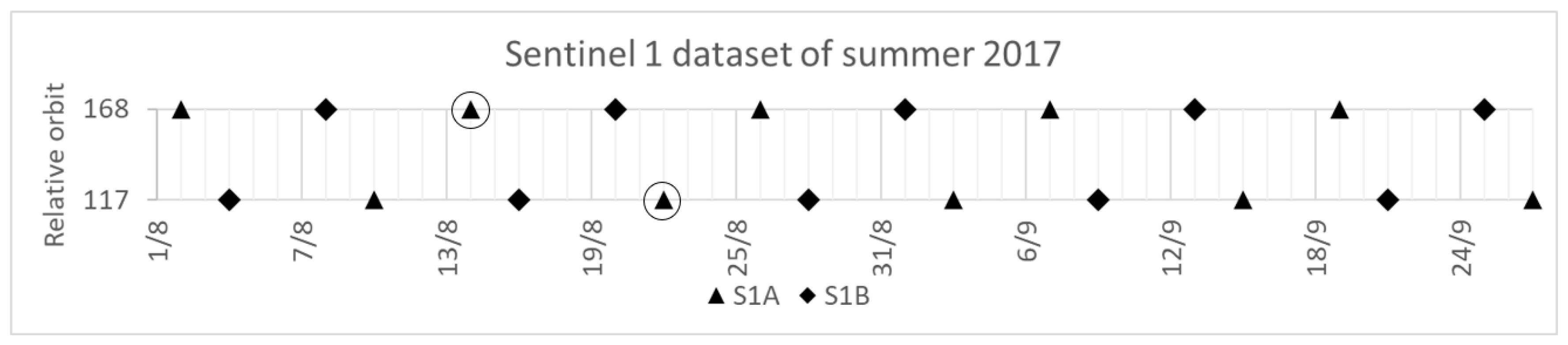
2.1. Study Area and Dataset

The proposed method was developed and tested over a mountainous area, encompassing the entire South Tyrol and the western part of Trentino (Italian Alps).
South Tyrol is located in the eastern Italian Alps (Figure 1). A rock glacier inventory (South Tyrol Inventory, STI) was recently compiled in this region, considering only the area located above 1600 m a.s.l. [16,41]. The landforms were identified and mapped using LIDAR (Light Detection and Ranging) DTMs (2.5 m GSD, Ground Sample Distance) and orthophotos of different dates. Descriptive features, both numerical and qualitative, were associated to each rock glacier, including a classification into active, inactive, and relict forms. The inventory includes 1665 rock glaciers, 230 of them (14%) were classified by the authors as active, 198 (12%) as inactive, 1099 (66%) as relict, and 138 (8%) were not classified (Figure 2a). Altitudinal and aspect distributions of active, inactive, and relict rock glaciers are shown in Figure 2b,c. The STI provided the landform outlines on which our analysis was developed. Moreover, the rock glaciers’ classification obtained by our method was compared with the classification provided by the inventory.
In Trentino, a set of 57 rock glaciers extracted from an inventory [15] (Figure 1) was used to validate the method (Section 3.3.), thanks to their activity status known from field observations [42], direct measurements [43], and visual analysis of multitemporal data. In detail, the visual analysis was conducted using high-resolution aerial orthophotos (2006 and 2014, 0.5 m and 0.2 m GSD, respectively) and LIDAR DTMs (2006 and 2013, 2 m and 0.5 m GSD, respectively). Geomorphological evidences such as the general deformation of the landform and the visible movements of large blocks were evaluated as signs of displacement. As a result, 29 rock glaciers were classified as moving (i.e., exhibiting certain evidence of surface movement) and 28 as no-moving (i.e., lacking surface movement).
Since the vegetation influences the effectiveness of our method (see Section 2.2.), over the Trentino all the rock glaciers were selected without vegetation cover. Over the South Tyrol, vegetated rock glaciers were recognized using a land cover map [44].
Two Sentinel-1 tracks, i.e., relative orbit 117 (ascending) and 168 (descending), cover the entire study area from 2014 (Figure 1a). The images were acquired in Interferometric Wide swath (IW) mode with a 250 km swath at 5 m by 20 m spatial resolution. Single Look Complex (SLC) product type and Vertical transmit Vertical receive (VV) polarization data were used for this analysis. The availability of both Sentinel-1A and 1B data ensure a temporal resolution of 6 days for each track. As the snow cover is a severe limitation for using satellite SAR data, our method was developed to analyze the activity of rock glaciers during the snow-free period, taking into account all the images covering the period from the beginning of August to the end of September 2017 (about 20 images, Figure 3). A LIDAR-derived DTM [45], with 2.5 m GSD was used to remove the topographic-related component during the SAR phase differences computation.
As additional independent dataset to evaluate the results, we used a permafrost probability map available from the GLOBpermafrost project [46] (Figure 1a). This dataset was produced by using satellite data, land cover information, and ground surface temperature [47], without considering the rock glacier location. Information on permafrost distribution at a global scale, with a spatial resolution of 1 Km, are provided by a numerical index ranging from 0 to 1. The higher is the index, the higher is the probability that permafrost exists in a given area.

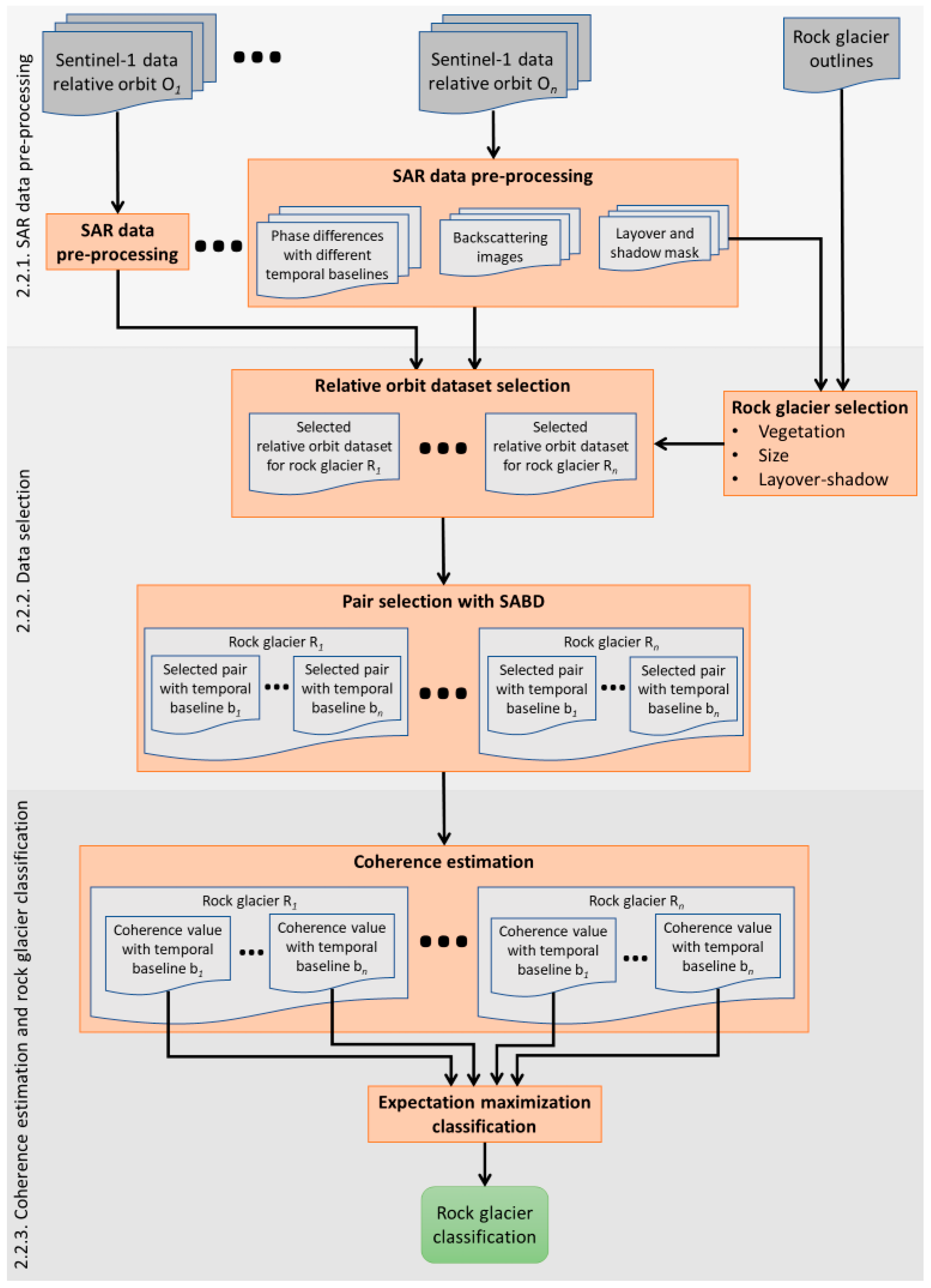
2.2. Description of the Proposed Method

In order to fulfill the requirements of the activity classification of rock glaciers as envisaged in the former chapter (e.g., wide area, topographic issues, short snow-free period), we propose an original application of interferometric coherence as a key indicator of displacement, able to label a large number of rock glaciers with their activity features. For the purposes of our work and according to our exclusively kinematic approach, we adopted two classes of rock glaciers: (i) “moving” rock glaciers, i.e., those with displacement detectable by our method and (ii) “no-moving” rock glaciers, i.e., those with no detectable displacement. This classification assumes to aggregate from a kinematic point of view the “inactive” and “relict” classes proposed by Barsch [2] under the class “no-moving,” and the “active” class under the class “moving,” without considering the permafrost content.
The coherence is a measure of the similarity between a pair of images (i.e., master and slave) [48,49,50,51]. Although the coherence is usually estimated on regular kernel windows [52], in this work we used the rock glacier outlines as boundaries to compute this value. This was done to avoid the average estimation of coherence and the consequent bias toward higher coherence values due to the introduction of small areas of calculation. Furthermore, in this way each rock glacier can be associated with a single SAR coherence value, representative of the entire area of the landform. Low coherence values indicate low or no similarity between the images, and this may be due to (i) the presence of vegetation, (ii) changes of the target properties (i.e., changes of the physical ground conditions), and (iii) changes of surface shape (i.e., displacement) [34,50,51,53,54,55,56,57]. High coherence values indicate, instead, similarity between the images (i.e., no movement and no changes in the surface properties of the rock glacier). Low coherence values due to vegetation cover can be avoided excluding vegetated rock glaciers from the classification process, for example, by means of a high-resolution land cover map.
To distinguish if a low coherence value between two images was related to the surface displacement or to a change in the physical properties of the ground (e.g., soil moisture changes due to rainfall or melt water from summer wet snowfalls), we used the intensity of the backscattering inside the rock glacier outline. Indeed, the backscattering change between two images can be related to changes of (i) target shape, (ii) orientation, or (iii) dielectric properties of the ground [48,58]. Field and remote sensing observations demonstrated that the rock glacier displacements during the summer season is much lower than the resolution of Sentinel-1 images used in this work (20 m GSD) [24,25,26,34]. Therefore, assuming that changes in shape and orientation of the rock glaciers are much lower than the resolution of SAR images during the investigated period, the only source of backscattering change is the difference in the dielectric properties of the ground, which is mainly caused by changes in moisture due to rainfall or summer snowfalls [58,59]. Backscattering information can therefore be used as key indicator to select the most suitable SAR images (i.e., without rainfall or summer snowfalls) on which to compute the coherence.
The overall scheme followed to develop the method is shown in Figure 4, where the classification procedure is divided into three parts: the SAR data pre-processing, the data selection, and the coherence calculation and the classification.

2.2.1. SAR Data Pre-Processing

The Sentinel-1 SAR images were multi-looked with a window size of 4 in azimuth and coregistered [50,60]. Then, backscattering images and layover and shadow masks were generated. All the possible pairs of images with temporal baselines of 6, 12, 18, 24, 30, 36, 42, 48, and 54 days were combined, and for each pair the phase difference was computed between a master and a slave image. Topographic corrections for the phase difference and backscattering, as well as geolocation of the data were accomplished using LIDAR DTM and Precise Orbit Auxiliary Files [49,50,51,60,61,62]. Datasets of images from different relative orbits were available for the investigated area (i.e., relative orbits 117 and 168), providing different Line Of Sight (LOS). Therefore, the SAR data pre-processing was applied by computing backscattering, layover and shadow masks, and phase differences for each relative orbit dataset.

2.2.2. Data Selection

Depending on the rock glacier orientation, topographic effects such as layover and shadow can be reduced using a favorable satellite geometric view (i.e., ascending or descending) [51,63]. Therefore, for each rock glacier, the relative orbit dataset with the smallest layover and shadow areas and the largest number of SAR pixels inside the rock glacier boundary was selected for the classification procedure.
Rock glaciers covered by vegetation were excluded from the classification procedure. Over the South Tyrol, this was accomplished using a land cover map [44], which includes the vegetation classes “grass,” “shrubs,” and “wood.” In particular, we considered as vegetated the rock glaciers with more than 15% of the surface covered by at least one of these vegetation classes. As inactive and relict rock glaciers have no movement and are often densely covered by vegetation [28,64], we assumed that the vegetated rock glaciers excluded from our classification are not in motion, and therefore they were added to the class of no-moving at the end of the classification procedure.
As small rock glaciers are more affected by decorrelation effects [38] that reduce the reliability of coherence, we excluded those landforms with an area less than 80 SAR pixels from the analysis. Furthermore, also rock glaciers with a layover-shadow area larger than 50% of the total area were excluded. These thresholds were chosen as a trade-off among robustness, reliability of coherence estimation, and number of excluded rock glaciers, i.e., non-classified.
In order to use the most suitable images to estimate the coherence, we selected for each rock glacier and for each temporal baseline one pair of images (i.e., master and slave) with the most similar mean backscattering values related to a reference SAR backscattering image acquired under dry meteorological conditions. To operate this selection, we identified periods with no snowfall and rainfall events using the precipitation and snow depth data collected by 17 weather stations distributed over the investigated area between 2000 m and 3200 m a.s.l. In this way, one reference backscattering image for each of the two relative orbits covering the investigated area was selected. In particular, the reference backscattering image acquired on 22nd August 2017 was chosen for the track 117, and the image acquired on 14th August 2017 for the track 168 (Figure 3).
For each rock glacier, we computed the sum of the absolute backscattering differences (SABD) between the reference backscattering image and the master and slave images of each pair for any temporal baseline. The SABD was computed as follows (Equation (1)):
S A B D = | 10 ·   log 10 ( I r I m ) | + | 10 ·   log 10 ( I r I s ) |
where, inside the rock glacier outline, I r is the mean intensity value of backscattering of the reference image and I m and I s are the mean intensity values of backscattering of the master and slave images, respectively. The lower the SABD value, the higher physical ground conditions similarity between the reference image and the pair of images. Then, for each rock glacier and for each temporal baseline, the pair of images with the lowest SABD value was selected to perform the coherence estimation.

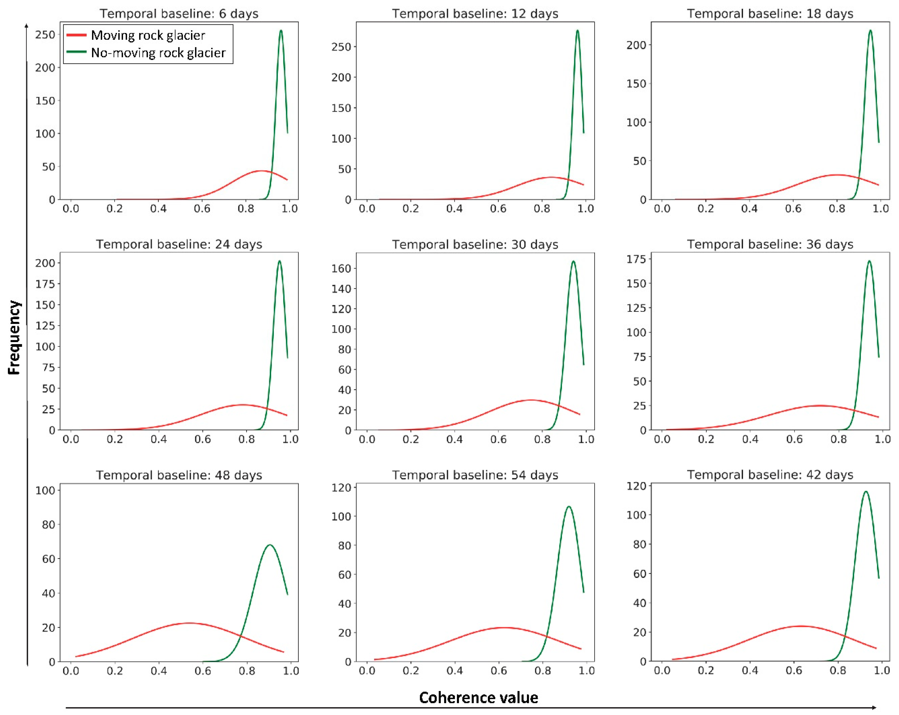
2.2.3. Coherence Estimation and Rock Glacier Classification

For the selected pairs of images, the coherence was estimated for each rock glacier using their outlines as follows [48] (Equation (2)):
C C = | i = 1 N r 1 i r 2 i   e j ( Δ φ i ) i = 1 N r 1 i 2 i = 1 N r 2 i 2   |
where r 1 i and r 2 i are the amplitudes of the complex signals of the master and slave at pixel i inside the rock glacier outline, Δ φ i is the phase difference obtained at pixel i inside the rock glacier area, and N is the number of pixels inside the rock glacier outlines. Therefore, one coherence value for each rock glacier and temporal baseline was estimated by using the selected pair of images.
Then, the unsupervised classification of rock glaciers was performed, labeling as “no-moving” the rock glaciers with high coherence values and as “moving” those with low coherence values. In particular, coherence values computed with long temporal baselines enabled to detect rock glaciers characterized by low movement rates, even if they are more affected by decorrelation effects unrelated with displacement [38,48,51,53,65]. On the contrary, coherence values computed with short baselines are less affected by decorrelation effects, but in this case small displacements are undetectable [35]. To identify the activity of a rock glacier, all the temporal baselines need to be exploited during the classification. In our method, this is done by using all the coherence values as features for an unsupervised classification based on Bayesian inferencing, thus avoiding having to select arbitrary thresholds. In detail, the well-known Expectation Maximization algorithm (EM) [66,67] was used as an iterative method to find the maximum likelihood estimates between moving and no-moving rock glaciers and select an adaptive decision threshold to minimize the overall classification error. Assuming that rock glaciers are spatially independent and that moving and a no-moving classes are represented by Gaussian distributions of the coherence values computed with different temporal baselines, the EM algorithm was applied for the activity classification (Figure 5).

2.3. Evaluation, Validation, and Performance Test

Assuming that moving rock glaciers are probably affected by permafrost, we adopted two different criteria to evaluate the classification results obtained with our method. The first criterion takes into account that the moving rock glaciers are expected to be located at higher altitudes with respect to the no-moving ones [14,20,23]. According to this assumption, the classified rock glaciers were plotted based on their altitudinal distribution. As a second evaluation criterion, we compared our classification with the permafrost probability map provided by the GLOBpermafrost project [46], expecting a higher permafrost probability for rock glaciers classified as moving.
To validate the method and highlight the wrongly-classified rock glaciers, we compared the results of our classification with the set of rock glaciers from Trentino, whose activity status was previously defined (Section 2.1.). We computed confusion matrices, accuracies (i.e., percent of correctly classified rock glaciers with respect to the total number) and Kappa coefficient. The last one is a more robust measure than simple percent accuracy calculation, because it takes into account the possibility of the accuracy occurring by chance. The coefficient ranges between 0 and 1, the higher the value, the higher is the quality of the classification. Good classifications have kappa coefficient higher than 0.6 [68].
A large and suitable dataset of SAR images is not always available for high mountain regions, where the snow-free period can be very short. Therefore, in order to simulate the conditions of a region with an extended snow cover period, we tested the performance of our method on a shorter period, using Sentinel-1 images acquired in only one, snow-free month. We performed two separate tests, using images from August and September 2017; hence the maximum temporal baseline available was 24 days. As with the former complete dataset, the analysis was performed on the whole study area and the results were validated on the set of rock glaciers from Trentino.

3. Results

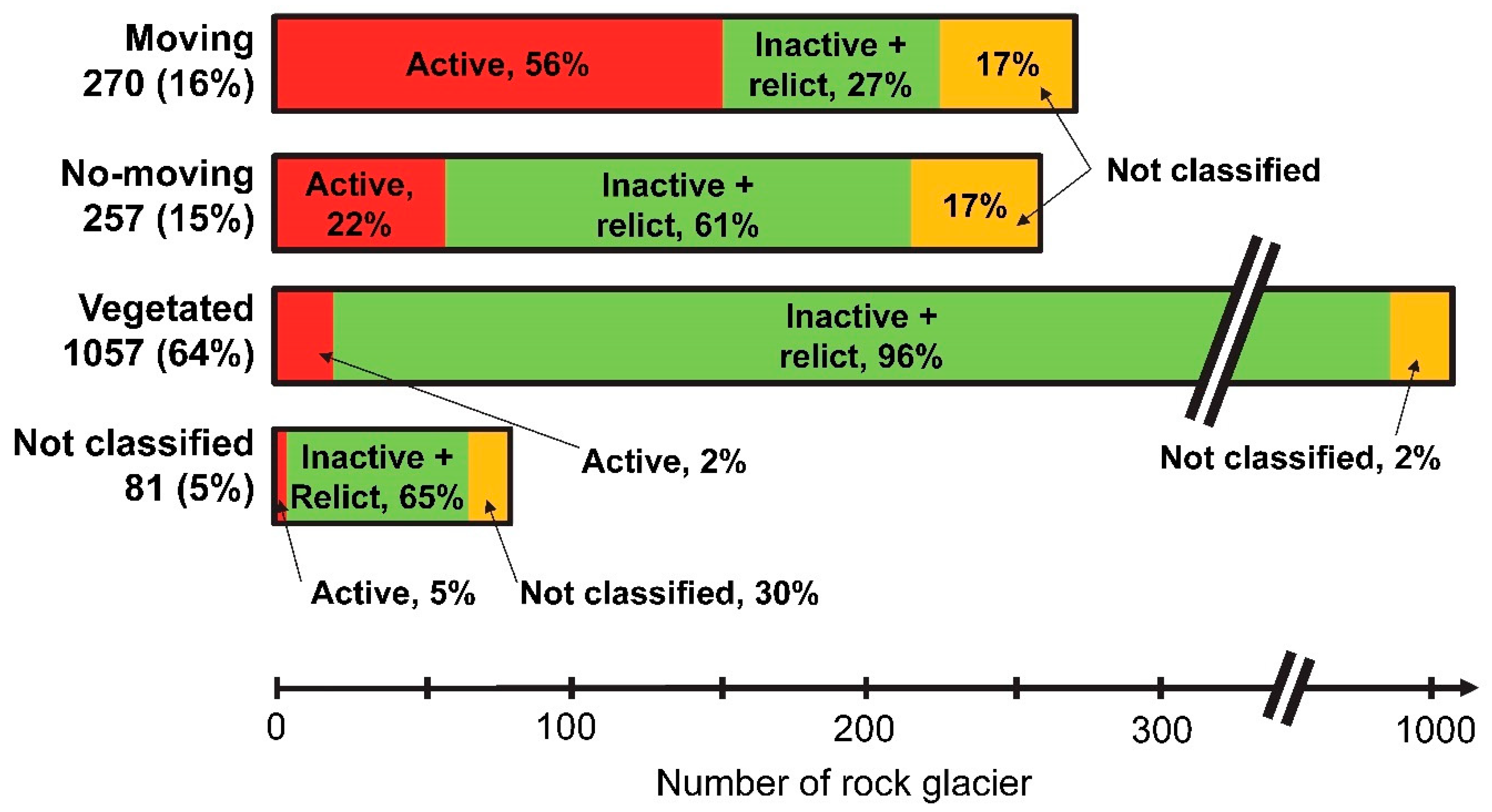
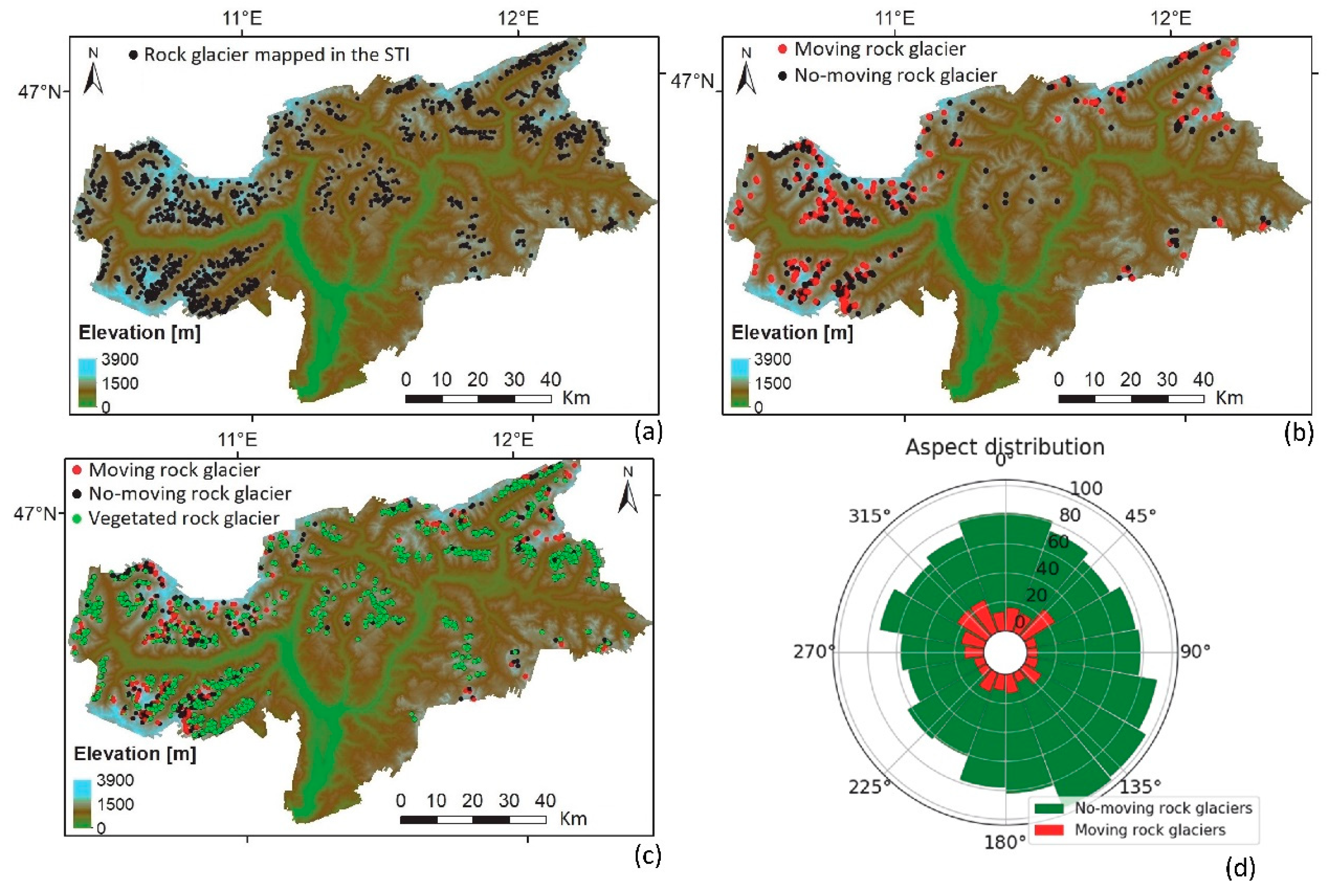
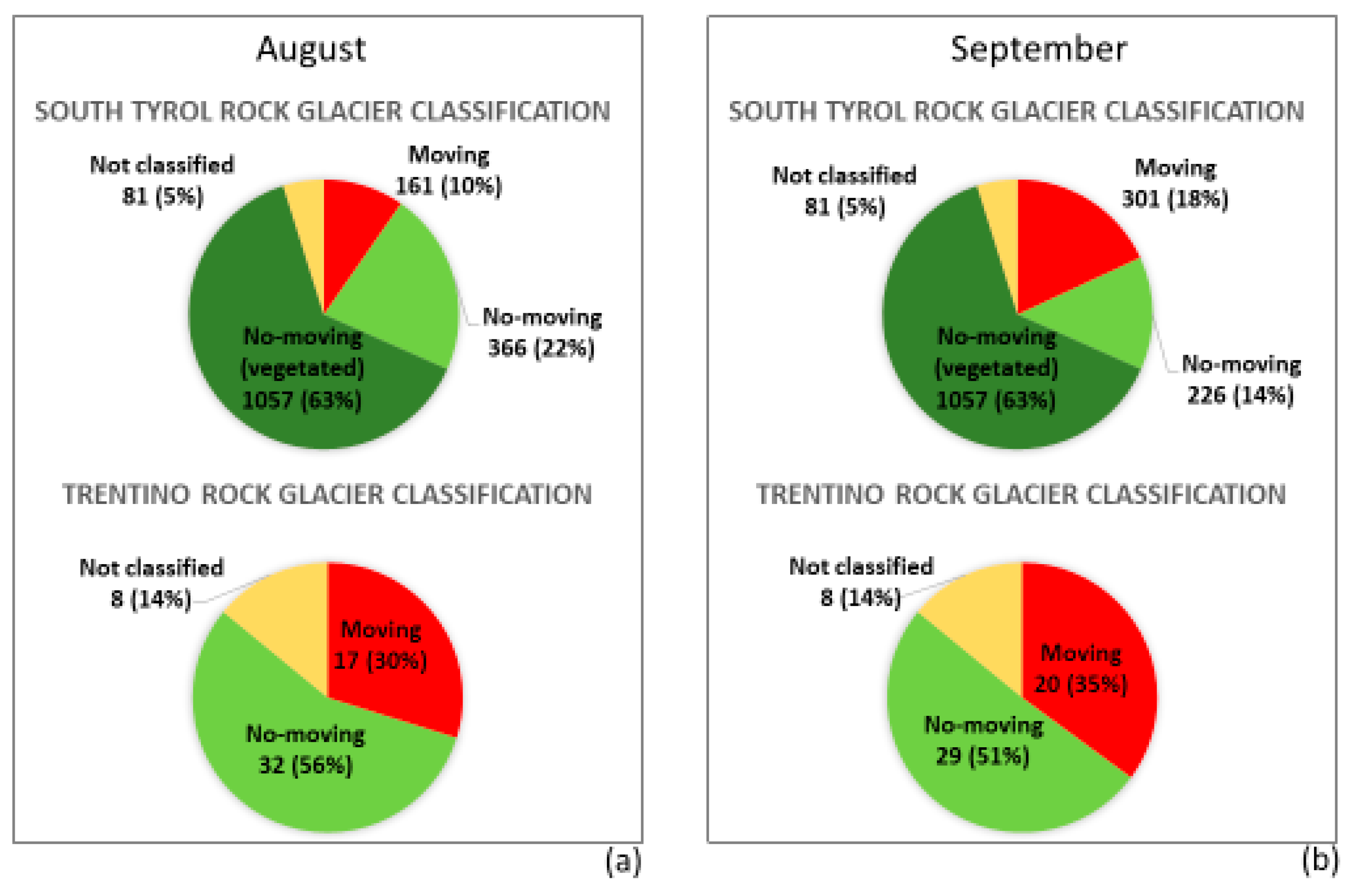
3.1. Rock Glaciers Classification and Comparison with the South Tyrol Inventory

In this section, we present the rock glacier classification using the landforms mapped in the STI. In addition, we show the comparison between our activity classification and that provided by the STI.
Out of the 1665 rock glaciers included in the inventory, more than 500 landforms were classified by our method. The remaining rock glaciers were not classified because they are covered by vegetation (1057), are too small (73), are in layover and shadow conditions (1), or are in both the two last conditions (7). According to our method, 270 rock glaciers were classified as moving and 257 as no-moving (Figure 6 and Figure 7b). The 1057 vegetated rock glaciers excluded from our classification were added to the class of no-moving (Figure 7c) (Section 2.2.2.). This assumption is supported by the classification of the STI, for which the 96% of the 1057 vegetated rock glaciers are labeled as inactive and relict (Figure 6).
The comparative analysis between our classification and that included in the STI was carried out comparing our moving class with the active rock glaciers of the inventory, and our no-moving class with the inactive and relict. Out of the 270 rock glaciers classified as moving by our method, in the STI, 152 (56%) were classified as active, i.e., in classification agreement, and 72 (27%) as inactive or relict, i.e., disagreement (Figure 6). The remaining (17%) were not labeled and only our classification could provide the activity information. We classified 257 rock glaciers as no-moving, and the agreement with STI (i.e., rock glaciers labeled as inactive and relict) is 61%. The disagreement of 22% consists of rock glaciers, which were labeled as active in the STI, while the remaining 17% of rock glaciers in the STI were not labeled. Among the 81 rock glaciers not classified by our method, 4 (5%) were classified as active in the STI, 53 (65%) as inactive or relict, and 24 (30%) were not classified.

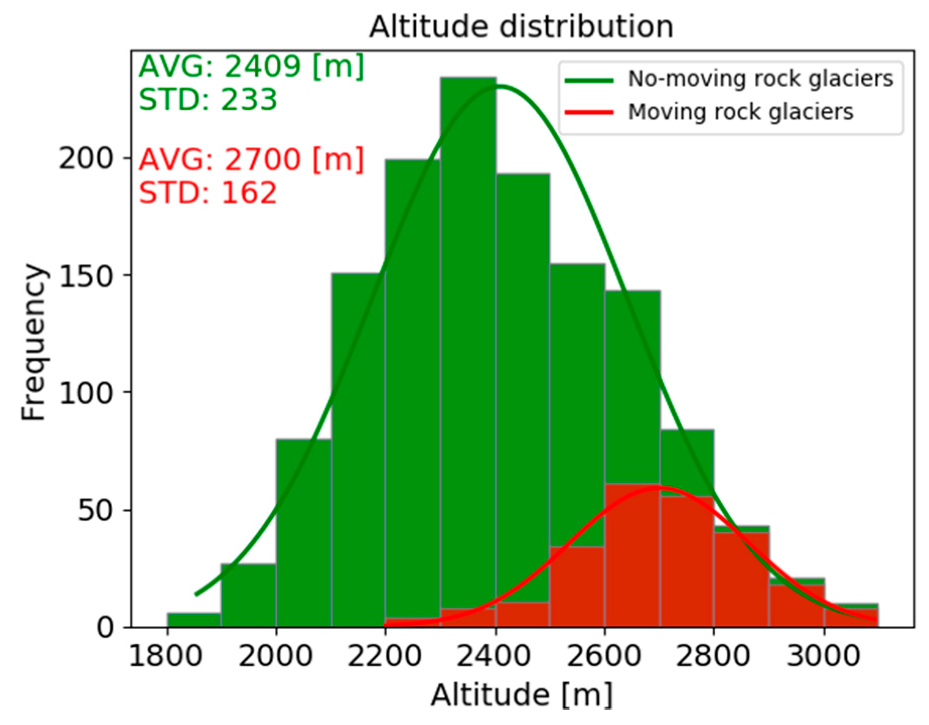
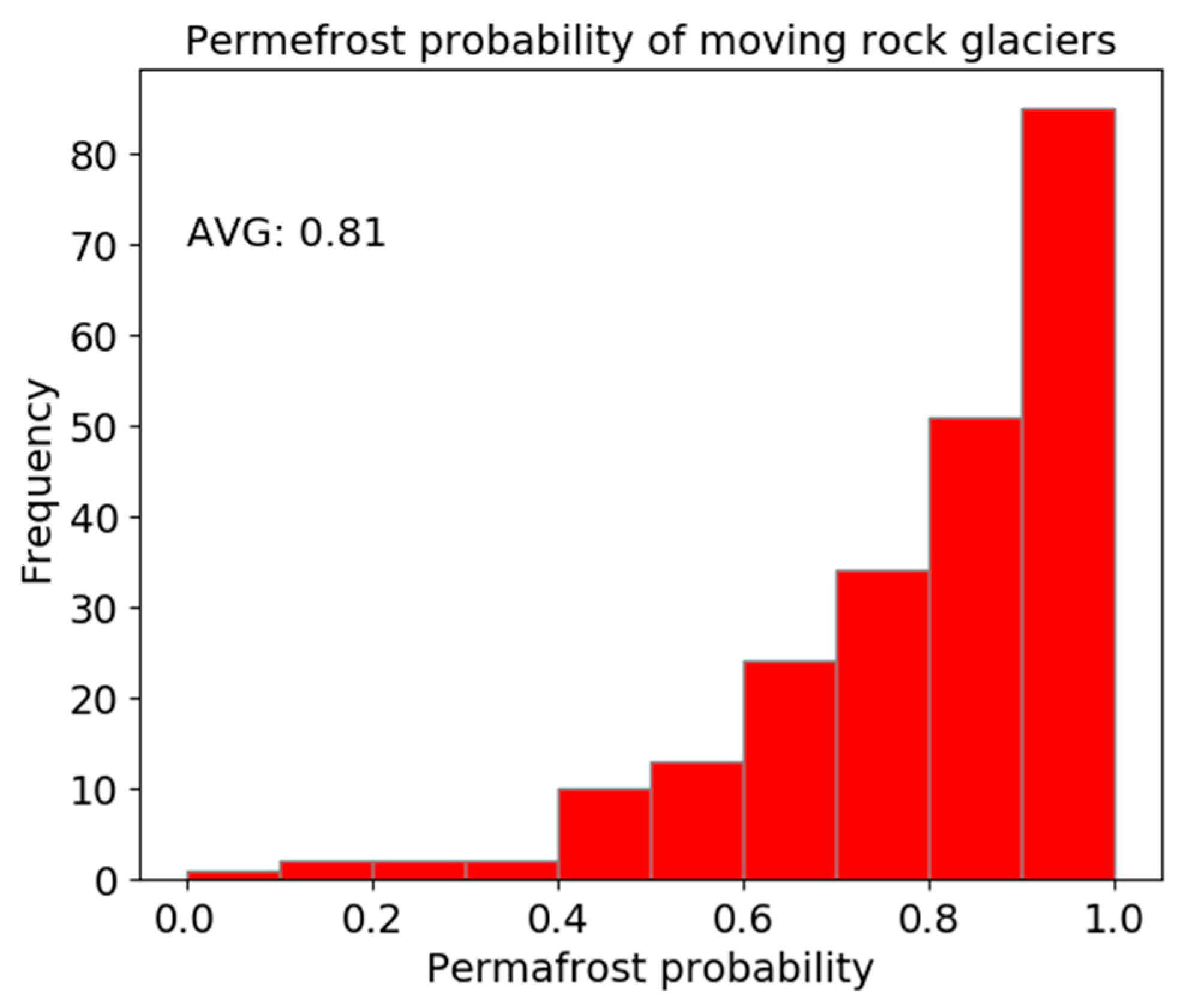
3.2. Evaluation of the Rock Glacier Classification with Altitude and Permafrost Probability

According to the first evaluation criterion (Section 2.3.), the classified rock glaciers were plotted based on their altitudinal distribution (Figure 8), including the vegetated landforms added to the no-moving class. Landforms classified as no-moving are located at an altitude between 1800 and 3100 m, with a mean of 2409 m, whereas the moving landforms are located between 2200 and 3100 m of altitude, with a mean altitude of 2700 m. Rock glaciers classified as moving are therefore located 300 m above the no-moving ones, and this difference supports the robustness of our analyses.
For the second evaluation criterion, we plotted the permafrost probability distribution of moving rock glaciers (Figure 9). According to the probability map, the rock glaciers classified as moving are located in areas with high permafrost probability values, with an average of 0.81. A small number of moving rock glaciers show low permafrost probability values (i.e., 17 rock glaciers have values lower than 0.5). The low permafrost probability of some rock glaciers may be due to a combination of classification errors and the low resolution of the permafrost probability map (1 Km).

3.3. Validation with the Trentino Dataset

Out of the 57 rock glaciers of Trentino, 21 were classified as moving and 28 as no-moving (Table 1). The remaining (8 rock glaciers) were not classified because they are too small (less than 80 SAR pixels) or have a layover or shadowing area higher than 50%. The validation results display an accuracy of 88% and a Kappa coefficient of 0.76 (Table 1). The number of rock glaciers misclassified as no-moving by our method (5) is overestimated with respect to the number of those misclassified as moving (1).

3.4. Performance Test with a Restricted Dataset of Images

Using only the images of August 2017, 161 rock glaciers were classified as moving and 366 as no-moving in South Tyrol (Figure 10a). The validation results obtained using the Trentino rock glaciers provided an accuracy value of 71% and a Kappa coefficient of 0.43, both being lower than the values obtained using the complete dataset (Table 1). The confusion matrix shows that our method correctly classified 14 rock glaciers as moving and 21 as no-moving, whereas the misclassification consists of 11 rock glaciers labeled as no-moving and 3 rock glaciers labeled as moving (Table 2).
The second performance test was conducted using only the images acquired in September 2017. In South Tyrol, 301 rock glaciers were classified as moving and 226 as no-moving (Figure 10b). The validation performed using the set of Trentino rock glaciers showed an accuracy value of 86% and a Kappa coefficient of 0.72, which are only slightly lower than those obtained with the complete dataset (Table 1). As shown by the confusion matrix (Table 2), our method correctly classified 42 rock glaciers (19 as moving and 23 as no-moving), whereas the misclassification consists of 7 rock glaciers. Therefore, using a restricted dataset of images, the no-moving rock glaciers are overestimated, and the accuracies and kappa coefficients are overall lower than those obtained with the complete dataset.
As a useful example to clarify the better results of the tests conducted with the restricted datasets of images, the SABD and the coherence trends for two rock glaciers of Trentino recognized as moving (Section 2.1.) were plotted over time for three temporal baselines (6, 12, and 18 days) (Figure 11). Results showed three evidences. First, an overall decrease in the coherence values by increasing the temporal baseline is observable. Second, as expected, an opposite trend between the SABD and the coherence is visible. In particular, a decrease in the coherence values from August to September is visible, especially for the shorter temporal baselines (i.e., 6 and 12 days). Third, despite a SABD trend is observable, the SABD difference over time between the images selected by our method (using both the complete and reduced datasets) is very low, compared to the total variation.
The coherence trends shown in Figure 11a are referred to a rock glacier classified as moving using both the complete dataset (two months) and the reduced dataset (August or September 2017). A decrease in the coherence values from August to September is visible along with a slight increase of SABD. The example shown in Figure 11b is referred to a rock glacier classified as no-moving in the August images, and as moving in the September images. For each temporal baseline, the coherence values of the images selected for August are higher than those of September and this may explain the different classification. This rock glacier was classified as moving using the complete dataset, despite the images selected for the complete dataset (red circles) are the same to those selected for the reduced dataset of August (red diamonds). This different classification is due to the larger temporal baselines (i.e., 30, 36, 42, 48, and 54 days) used with the complete dataset.

4. Discussion

In this work, a SAR-based, unsupervised method to classify the activity of rock glaciers was developed. The potential of the interferometric SAR coherence of Sentinel-1 images was exploited to distinguish moving and no-moving landforms over large mountainous areas. We developed and tested our method in the Eastern Italian Alps, where the geographical location and the outline of rock glaciers was extracted from existing inventories [15,16].
As suggested by Villarroel et al. [35], the information on the activity of rock glaciers can be derived from the analysis of multitemporal optical data and the interpretation of geomorphological evidences, such as, among others, inclination of the frontal slope, presence or absence of vegetation, and degree of development of furrows and ridges over the rock glacier surface. However, one of the main weaknesses of such criteria is that they are based on subjective interpretations and can therefore lead to erroneous interpretations. At a large scale, displacement information can be obtained using differential interferometry [28,33,36,37,38,69,70]. SAR data processing through the interferometric techniques is often difficult in high mountain regions, especially for the unwrapping processes [35,38]. Our coherence-based method is able to solve the erroneous interpretation due to the subjective analysis of geomorphological evidences, avoiding at the same time the complicated unwrapping processes.
A SAR-based approach such as that used in our work is affected by layover and shadow effects because of the SAR imaging geometry and the complex topography of high mountain regions [60,71]. Consequently, extended areas with these effects can potentially decrease the number of landforms that can be investigated. In order to reduce these effects, Rott et al. [71] and Strozzi et al [28] suggest the use of the most appropriate image geometries (i.e., ascending and descending) depending on the orientation of the objects to be investigated. In this work, two datasets with different relative orbits were used, thus increasing the number of classified rock glaciers by using the most appropriate geometry. Indeed, our findings show that, exploiting the relative orbit 117 and 168 (Figure 1a), only 17% of all the investigated rock glaciers were excluded because of extensive layover and shadow effects. Therefore, at a large scale, a key element to reduce the number of unclassified landforms is the use of different relative orbit datasets.
In our work, an original application of the interferometric coherence, estimated with different temporal baselines, was used to investigate the activity of rock glaciers. To define the activity status of rock glaciers, the strength of our approach relies in the use of the interferometric coherence, which can be easily estimated. Other widely used interferometric approaches, such as the DIn-SAR, allow obtaining displacement maps, from which the activity of rock glaciers could be indirectly estimated by visual interpretation [28,36,70]. However, although these approaches are the most established, they could be somewhat subjective and may lead to misinterpretations. Therefore, our approach may help overcome these limitations.
An innovative point of our method is the use of the rock glacier outlines as boundaries to estimate the coherence, which is usually estimated using regular kernel windows [52,60]. In order to avoid the averaging estimation of coherence in the kernel window and the possible biases toward higher coherence values, we estimated the coherence using as window the outline of the rock glaciers (Equation (2)). The single estimated SAR coherence value is therefore representative of the entire area of each investigated rock glacier. However, this outline-dependent approach requires an accurate definition of the rock glacier perimeters, and this may represent a limitation if this is poorly accomplished. Indeed, the use of inaccurate rock glacier outlines (e.g., perimeters excluding parts of the landform or including external parts) may conduct to non-representative coherence measure, thus making an incorrect classification. Currently, the geographical outlines can be drawn from the analysis of orthophotos and DTMs (e.g., [14,15,18]); however, the criteria to map the rock glaciers are still not standardized and large margins of uncertainty and subjectivity still remain [72]. In the inventories used for our work [15,16], the landforms were also mapped from the interpretation of aerial orthophotos and DTMs. The experience and training of the operators in compiling these good quality inventories have contributed to reduce the potential misclassifications due to the coarse definition of the rock glacier outlines.
The validation procedure with the Trentino dataset highlighted a slight overestimation of rock glaciers classified as no-moving by our method. This can be explained by three reasons.
The first is the SAR geometric view, because the LOS orientation compared to the rock glacier orientation is frequently not favorable to detect deformations [28,71]. For example, for those rock glaciers with the main axis aligned around the North–South direction, the displacement may not be detectable. Therefore, in correspondence to the North–South direction, no-moving rock glaciers could be overestimated. This limiting factor can be reduced by using the most appropriate SAR geometry depending on the rock glacier orientation [28,71]. In this work, we used two different geometries (i.e., relative orbits 117 and 168) and the results show that, in correspondence to the North–South direction, no-moving rock glaciers are not overestimated, with the number of moving rock glaciers not strongly reduced (89 moving rock glaciers are distributed around the North–South direction ± 30°, Figure 7d). Therefore, in our work, the SAR geometric view cannot explain the observed overestimation of no-moving rock glaciers.
The second reason is the particular spatial displacement pattern that characterizes some rock glaciers. As suggested by Touzi et al. [52], a homogeneous displacement inside the boundary used to estimate the coherence does not lead to a decrease in the coherence value. Therefore, rock glaciers exhibiting a homogeneous displacement pattern are classified as no-moving, because the coherence values estimated in their perimeter do not decrease over time. This kind of displacement pattern was recognized for small- to medium-sized rock glaciers composed by a single debris lobe, which moves with similar velocities over time. They were called “monomorphic” rock glaciers by Frauenfelder and Kääb [73]. Some of them were identified from multitemporal orthophotos and DTMs in the Trentino dataset, and this may partly explain the resulting overestimation of no-moving rock glaciers in the validation procedure.
The third reason is the existence of rock glaciers with very small displacement rates, that could not be detected using short temporal baselines [60]. To detect small displacements, Villarroel et al. [35] suggest using large temporal baselines (e.g., up to 60 days). In our work, different baselines were used, and the overestimation of no-moving rock glaciers was reduced using the larger ones (e.g., 30, 36, 42, 48, and 54 days), with the ability to detect very small displacements as well. Indeed, our findings showed that, among the three classification tests conducted using (i) the complete dataset of Sentinel-1 images, (ii) the images acquired only in August and (iii) those acquired only in September, the best classification performance was obtained using the complete dataset, and the number of no-moving rock glaciers was slightly overestimated using the two restricted datasets. For example, a rock glacier from the Trentino dataset surveyed with a laser total station and having an average velocity of 0.09 m y−1 [43] was classified as moving using the complete dataset, while using the images acquired only in August (maximum temporal baseline of 24 days) the displacement was not detected.
On the contrary, an overestimation of moving rock glaciers could be generated by the presence of vegetation, because decorrelation effects due to vegetation reduce the coherence values [74,75]. To mitigate this problem, heavily vegetated rock glaciers can be excluded from the processing by using, if available, a land cover map, as was done in our work. Alternatively, the Normalized Difference Vegetation Index (NDVI) can also be used. In this work, an overestimation of moving rock glaciers was not observed. A negligible number of rock glaciers were misclassified as no-moving by our method (Table 1 and 2), probably because of decorrelation effects unrelated with the displacement [51,53,65].
An alternative hypothesis that can partly explain the observed overestimations can be due to possible switch of the rock glaciers’ activity level in the period of the visual analysis conducted on Trentino (2006–2014) and the period investigated by SAR images (summer 2017). However, changes in the level of activity are not expected in such a short period, and this is supported by the direct measurements conducted on two rock glaciers [43].
The two rock glaciers used as examples in the Section 3.4. showed a decrease in the coherence values from August to September (Figure 11). This loss of coherence may be explained by a different activity behavior of the two landforms, with a possible acceleration in the last part of the investigated period (i.e., in September). The number of studies documenting variations in rock glacier velocity over short periods (i.e., seasonal or sub-seasonal) is very limited. However, recent continuous measurements conducted on some rock glaciers in the Alps [26,76] suggest sub-seasonal velocity variations, with an increase during the summer and maximum velocities at the beginning of autumn. Therefore, our findings suggest that, at least for the two investigated landforms, the decreasing trend of the coherence is probably related to an increase of sub-seasonal displacements and demonstrate that the coherence is sensitive to short-term displacement variations.
Among the two classification tests conducted by using the restricted dataset of Sentinel-1 images (i.e., the images acquired only in August and only in September), the validation procedure with the Trentino dataset obtained the best performance using the images of September, with an accuracy of 86% and a kappa coefficient of 0.72. In August, a higher overestimation of no-moving rock glaciers is observable. This result may be explained by the decrease in the coherence values from August to September observable from the two investigated rock glaciers (Figure 11). As rock glacier velocities increase during the summer, displacement rates are lower in August and higher in September. Therefore, rock glaciers moving at low velocities are easier identified in September because their displacement rates are higher than in August. This may have caused an overestimation of the no-moving rock glaciers in the analyses based on the August dataset.

5. Conclusions

In this study, an original, unsupervised method to classify the activity of rock glaciers by using a SAR remote sensing approach was developed. Backscattering and coherence of Sentinel-1 data were exploited in order to classify rock glaciers in moving (i.e., with detectable displacement) and no-moving (i.e., without detectable displacement). This method is applicable at a regional-scale, thus enabling the rock glacier classification over large areas, where only the geographical location of the landforms is known and no information about their activity is available. If a rock glacier inventory already includes the information on activity, our method is able to reduce the uncertainties and improve its reliability.
Our method was developed in South Tyrol, where 1665 rock glaciers were mapped within an inventory, and we classified 270 landforms as moving and 1314 as no-moving. The method was validated by using an independent dataset of rock glaciers from a neighboring area (Trentino), for which an accuracy of 88% and kappa coefficient of 0.76 was obtained.
We used an approach based on the SAR coherence, which has the main advantage to provide an objective detection of the rock glacier activity status, avoiding the subjectivity and the potential misinterpretations that characterize, for example, the visual interpretation of DIn-SAR products. In addition, a SAR coherence approach enables to overcome the complicated phase unwrapping process, required by the traditional DIn-SAR interferometry.
Further work is needed to exhaustively define the activity status of rock glaciers at a regional-scale (i.e., their activity and ice content), a key task that is still lacking in the inventories. Future work may involve the integration of the information on the activity obtained from our method with other approaches for ice content detection.

Author Contributions

Conceptualization, A.B. and M.C.; methodology, A.B., M.C., and C.M.; software, P.R., A.B., M.C., and C.M.; validation, A.B., M.C., R.S., and F.Z.; data curation, A.B.; writing—original draft preparation, A.B.; writing—review and editing, M.C., C.M., R.S., F.Z., C.N., and G.C.; supervision, M.C. and R.S.; project administration, G.C.; funding acquisition, G.C. and M.C.

Funding

This work was conducted within the project ALPSMOTION (ALPine Slow slope Movement moniTorIng and detectiON with remote and proximal sensing), coordinated by Eurac Research-Institute for Earth Observation and funded by the Autonomous province of Bolzano “Ripartizione Diritto allo Studio, Università e Ricerca Scientifica.” The PhD of A.B. in Earth and Environmental Sciences at the University of Pavia was funded by the ALPSMOTION project. The authors thank the Department of Innovation, Research and University of the Autonomous Province of Bozen/Bolzano for covering the Open Access publication costs.

Acknowledgments

The Sentinel-1 data were processed with SARscape software (SARMAP).

Conflicts of Interest

The authors declare no conflict of interest.

References

  1. Haeberli, W.; Hallet, B.; Arenson, L.; Elconin, R.; Humlum, O.; Kääb, A.; Kaufmann, V.; Ladanyi, B.; Matsuoka, N.; Springman, S.; et al. Permafrost creep and rock glacier dynamics. Permafr. Periglac. Process. 2006, 17, 189–214. [Google Scholar] [CrossRef]
  2. Barsch, D. Rockglaciers, Indicators for the Permafrost and Former Geoecology in High. Mountain Environment, Series in the Physical Environment; Springer: Berlin, Germany, 1996. [Google Scholar]
  3. Delaloye, R.; Lambiel, C.; Gärtner-Roer, I. Overview of rock glacier kinematics research in the Swiss Alps. Geogr. Helv. 2010, 65, 135–145. [Google Scholar] [CrossRef]
  4. Lugon, R.; Stoffel, M. Rock-glacier dynamics and magnitude-frequency relations of debris flows in a high-elevation watershed: Ritigraben, Swiss Alps. Glob. Planet. Change 2010, 73, 202–210. [Google Scholar] [CrossRef]
  5. Delaloye, R.; Morard, S.; Barboux, C.; Abbet, D.; Gruber, V.; Riedo, M.; Gachet, S. Rapidly moving rock glaciers in Mattertal. Jahrestagung Schweizerischen Geomorphology Gesellschaft 2012, 29, 21–31. [Google Scholar]
  6. Scotti, R.; Crosta, G.B.; Villa, A. Destabilisation of creeping permafrost: The plator rock glacier case study (central Italian Alps). Permafr. Periglac. Process. 2017, 28, 224–236. [Google Scholar] [CrossRef]
  7. Bodin, X.; Krysiecki, J.-M.; Schoeneich, P.; Le Roux, O.; Lorier, L.; Echelard, T.; Peyron, M.; Walpersdorf, A. The 2006 Collapse of the bérard rock glacier (southern French Alps). Permafr. Periglac. Process. 2017, 28, 209–223. [Google Scholar] [CrossRef]
  8. Marcer, M.; Serrano, C.; Brenning, A.; Bodin, X.; Goetz, J.; Schoeneich, P. Evaluating the destabilization susceptibility of active rock glaciers in the French Alps. Cryosphere 2019, 13, 141–155. [Google Scholar] [CrossRef] [Green Version]
  9. Vivero, S.; Lambiel, C. Monitoring the crisis of a rock glacier with repeated UAV surveys. Geogr. Helv. 2019, 74, 59–69. [Google Scholar] [CrossRef]
  10. Kääb, A.; Frauenfelder, R.; Roer, I. On the response of rockglacier creep to surface temperature increase. Glob. Planet. Change 2007, 56, 172–187. [Google Scholar] [CrossRef]
  11. Alcántara, I.; Goudie, A. Geomorphological Hazards and Disaster Prevention; Cambridge University Press: Cambrige, UK, 2010. [Google Scholar]
  12. Cremonese, E.; Gruber, S.; Phillips, M.; Pogliotti, P.; Boeckli, L.; Noetzli, J.; Suter, C.; Bodin, X.; Crepaz, A.; Kellerer-Pirklbauer, A.; et al. Brief communication: “An inventory of permafrost evidence for the European Alps”. Cryosphere 2011, 5, 651–657. [Google Scholar] [CrossRef]
  13. Colucci, R.R.; Boccali, C.; Žebre, M.; Guglielmin, M. Rock glaciers, protalus ramparts and pronival ramparts in the south-eastern Alps. Geomorphology 2016, 269, 112–121. [Google Scholar] [CrossRef]
  14. Scotti, R.; Brardinoni, F.; Alberti, S.; Frattini, P.; Crosta, G.B. A regional inventory of rock glaciers and protalus ramparts in the central Italian Alps. Geomorphology 2013, 186, 136–149. [Google Scholar] [CrossRef]
  15. Seppi, R.; Carton, A.; Zumiani, M.; Dall’Amico, M.; Zampedri, G.; Rigon, R. Inventory, distribution and topographic features of rock glaciers in the southern region of the Eastern Italian Alps (Trentino). Geogr. Fis. Din. Quat. 2012, 35, 185–197. [Google Scholar]
  16. Mair, V.; Zischg, A.; Krainer, K.; Stötter, J.; Zilger, J.; Belitz, K.; Lang, K. PROALP Rilevamento e monitoraggio dei fenomeni permafrost. Esperienze della Provincia di Bolzano. Neve Valanghe 2008, 64, 50–59. [Google Scholar]
  17. Krainer, K.; Ribis, M. A rock glacier inventory of the Tyrolean Alps (Austria). Austrian J. Earth Sci. 2012, 105, 32–47. [Google Scholar]
  18. Roer, I.; Nyenhuis, M. Rockglacier activity studies on a regional scale: Comparison of geomorphological mapping and photogrammetric monitoring. Earth Surf. Process. Landforms 2007, 32, 1747–1758. [Google Scholar] [CrossRef]
  19. Falaschi, D.; Tadono, T.; Masiokas, M. Rock glaciers in the patagonian andes: An inventory for the monte san lorenzo (cerro cochrane) massif, 47° s. Geogr. Ann. Ser. A Phys. Geogr. 2015, 97, 769–777. [Google Scholar] [CrossRef]
  20. Onaca, A.; Ardelean, F.; Urdea, P.; Magori, B. Southern Carpathian rock glaciers: Inventory, distribution and environmental controlling factors. Geomorphology 2017, 293, 391–404. [Google Scholar] [CrossRef]
  21. Rangecroft, S.; Harrison, S.; Anderson, K.; Magrath, J.; Castel, A.P.; Pacheco, P. A First rock glacier inventory for the Bolivian Andes. Permafr. Periglac. Process. 2014, 25, 333–343. [Google Scholar] [CrossRef]
  22. Blöthe, J.H.; Rosenwinkel, S.; Höser, T.; Korup, O. Rock-glacier dams in High Asia. Earth Surf. Process. Landforms 2019, 44, 808–824. [Google Scholar] [CrossRef]
  23. Jones, D.B.; Harrison, S.; Anderson, K.; Selley, H.L.; Wood, J.L.; Betts, R.A. The distribution and hydrological significance of rock glaciers in the Nepalese Himalaya. Glob. Planet. Change 2018, 160, 123–142. [Google Scholar] [CrossRef]
  24. Strozzi, T.; Delaloye, R.; Kääb, A.; Ambrosi, C.; Perruchoud, E.; Wegmüller, U. Combined observations of rock mass movements using satellite SAR interferometry, differential GPS, airborne digital photogrammetry, and airborne photography interpretation. J. Geophys. Res. Earth Surf. 2010, 115, 1–11. [Google Scholar] [CrossRef]
  25. Buchli, T.; Kos, A.; Limpach, P.; Merz, K.; Zhou, X.; Springman, S.M. Kinematic investigations on the Furggwanghorn Rock Glacier, Switzerland. Permafr. Periglac. Process. 2018, 29, 3–20. [Google Scholar] [CrossRef]
  26. Wirz, V.; Gruber, S.; Purves, R.S.; Beutel, J.; Gärtner-Roer, I.; Gubler, S.; Vieli, A. Short-term velocity variations at three rock glaciers and their relationship with meteorological conditions. Earth Surf. Dyn. 2016, 4, 103–123. [Google Scholar] [CrossRef] [Green Version]
  27. Kaab, A. Photogrammetry for early recognition of high mountain hazards: New techniques and applications. Phys. Chem. Earth Part B Hydrol. Ocean. Atmos. 2000, 25, 765–770. [Google Scholar] [CrossRef]
  28. Strozzi, T.; Kääb, A.; Frauenfelder, R. Detecting and quantifying mountain permafrost creep from in situ inventory, space-borne radar interferometry and airborne digital photogrammetry. Int. J. Remote Sens. 2004, 25, 2919–2931. [Google Scholar] [CrossRef]
  29. Kääb, A.; Vollmer, M. Surface geometry, thickness changes and flow fields on creeping mountain permafrost: Automatic extraction by digital image analysis. Permafr. Periglac. Process. 2000, 11, 315–326. [Google Scholar] [CrossRef]
  30. Monnier, S.; Kinnard, C. Pluri-decadal (1955–2014) evolution of glacier-rock glacier transitional landforms in the central Andes of Chile. Earth Surf. Dynam. 2017, 5, 493–509. [Google Scholar] [CrossRef]
  31. Kenyi, L.W.; Kaufmann, V. Estimation of rock glacier surface deformation using sar interferometry data. IEEE Trans. Geosci. Remote Sens. 2003, 41, 1512–1515. [Google Scholar] [CrossRef]
  32. Lugon, R.; Lambiel, C.; Raetzo, H. ERS InSAR for assessing rock glacier activity. In Proceedings of the Ninth International Conference on Permafrost, University of Alaska, Fairbanks, Fairbanks, AK, USA, 29 June–3 July 2008. [Google Scholar]
  33. Barboux, C.; Strozzi, T.; Delaloye, R.; Wegmüller, U.; Collet, C. Mapping slope movements in Alpine environments using TerraSAR-X interferometric methods. ISPRS J. Photogramm. Remote Sens. 2015, 109, 178–192. [Google Scholar] [CrossRef] [Green Version]
  34. Necsoiu, M.; Onaca, A.; Wigginton, S.; Urdea, P. Rock glacier dynamics in Southern Carpathian Mountains from high-resolution optical and multi-temporal SAR satellite imagery. Remote Sens. Environ. 2016, 177, 21–36. [Google Scholar] [CrossRef] [Green Version]
  35. Villarroel, C.; Tamburini Beliveau, G.; Forte, A.; Monserrat, O.; Morvillo, M.; Villarroel, C.D.; Tamburini Beliveau, G.; Forte, A.P.; Monserrat, O.; Morvillo, M. DInSAR for a Regional inventory of active rock glaciers in the dry andes mountains of argentina and chile with sentinel-1 data. Remote Sens. 2018, 10, 1588. [Google Scholar] [CrossRef]
  36. Liu, L.; Millar, C.I.; Westfall, R.D.; Zebker, H.A. Surface motion of active rock glaciers in the Sierra Nevada, California, USA: Inventory and a case study using InSAR. Cryosphere 2013, 7, 1109–1119. [Google Scholar] [CrossRef]
  37. Wang, X.; Liu, L.; Zhao, L.; Wu, T.; Li, Z.; Liu, G. Mapping and inventorying active rock glaciers in the northern Tien Shan of China using satellite SAR interferometry. Cryosphere 2017, 11, 997–1014. [Google Scholar] [CrossRef] [Green Version]
  38. Barboux, C.; Delaloye, R.; Lambiel, C. Inventorying slope movements in an Alpine environment using DInSAR. Earth Surf. Process. Landforms 2014, 39, 2087–2099. [Google Scholar] [CrossRef] [Green Version]
  39. Ferretti, A.; Prati, C.; Rocca, F. Permanent scatterers in SAR interferometry. IEEE Trans. Geosci. Remote Sens. 2001, 39, 8–20. [Google Scholar] [CrossRef]
  40. Berardino, P.; Fornaro, G.; Lanari, R.; Sansosti, E. A new algorithm for surface deformation monitoring based on small baseline differential SAR interferograms. IEEE Trans. Geosci. Remote Sens. 2002, 40, 2375–2383. [Google Scholar] [CrossRef] [Green Version]
  41. Zischg, A.; Mair, V.; Lang, K. PROALP-KARTIERUNG und monitoring von Permafrost in der Autonomen Provinz Bozen Südtirol, Italien. In Proceeding of the 12th Congress INTERPRAEVENT 2012, Grenoble, France, 23–26 April 2012; pp. 421–432. [Google Scholar]
  42. Seppi, R.; University of Pavia, Pavia, Italy. Personal communication, 2019.
  43. Seppi, R.; Carturan, L.; Carton, A.; Zanoner, T.; Zumiani, M.; Cazorzi, F.; Bertone, A.; Baroni, C.; Salvatore, M.C. Decoupled kinematics of two neighbouring permafrost creeping landforms in the Eastern Italian Alps. Earth Surf. Process. Landforms. Accepted. [CrossRef]
  44. Land Use Information System South Tyrol. Available online: http://geoportale.retecivica.bz.it/geodati.asp (accessed on 20 February 2018).
  45. South Tyrol Digital Terrain Model (DTM). Available online: http://geoportale.retecivica.bz.it/geodati.asp (accessed on 20 February 2018).
  46. Bartsch, A.; Grosse, G.; Kääb, A.; Westermann, S.; Strozzi, T.; Wiesmann, A.; Duguay, C.; Seifert, F.M.; Obu, J.; Goler, R. GlobPermafrost—How space-based earth observation supports understanding of permafrost. In Proceedings of the ESA Living Planet Symposium, Prague, Czech Republic, 9–13 May 2016. [Google Scholar]
  47. Westermann, S.; Peter, M.; Langer, M.; Schwamborn, G.; Schirrmeister, L.; Etzelmüller, B.; Boike, J. Transient modeling of the ground thermal conditions using satellite data in the Lena River delta, Siberia. Cryosphere 2017, 11, 1441–1463. [Google Scholar] [CrossRef] [Green Version]
  48. Massonnet, D.; Souyris, J.-C. Imaging with Synthetic Aperture Radar; EPFL Press: Lausanne, Switzerland, 2008. [Google Scholar]
  49. Moreira, A.; Prats-Iraola, P.; Younis, M.; Krieger, G.; Hajnsek, I.; Papathanassiou, K.P. A tutorial on synthetic aperture radar. IEEE Geosci. Remote Sens. Mag. 2013, 1, 6–43. [Google Scholar] [CrossRef] [Green Version]
  50. Yague-Martinez, N.; Prats-Iraola, P.; Rodriguez Gonzalez, F.; Brcic, R.; Shau, R.; Geudtner, D.; Eineder, M.; Bamler, R. Interferometric Processing of Sentinel-1 TOPS data. IEEE Trans. Geosci. Remote Sens. 2016, 54, 2220–2234. [Google Scholar] [CrossRef]
  51. Klees, R.; Massonnet, D. Deformation measurements using SAR interferometry: Potential and limitations. Geol. Mijnb. 1998, 77, 161–176. [Google Scholar] [CrossRef]
  52. Touzi, R.; Lopes, A.; Bruniquel, J.; Vachon, P.W. Coherence estimation for SAR imagery. IEEE Trans. Geosci. Remote Sens. 1999, 37, 135–149. [Google Scholar] [CrossRef] [Green Version]
  53. Corbane, C.; Lemoine, G.; Pesaresi, M.; Kemper, T.; Sabo, F.; Ferri, S.; Syrris, V. Enhanced automatic detection of human settlements using Sentinel-1 interferometric coherence. Int. J. Remote Sens. 2018, 39, 842–853. [Google Scholar] [CrossRef]
  54. Massonnet, D.; Feigl, K.L. Radar interferometry and its application to changes in the Earth’s surface. Rev. Geophys. 1998, 36, 441–500. [Google Scholar] [CrossRef]
  55. Smith, L.C. Emerging applications of interferometric synthetic aperture radar (InSAR) in geomorphology and hydrology. Ann. Assoc. Am. Geogr. 2002, 92, 385–398. [Google Scholar] [CrossRef]
  56. Nolan, M.; Fatland, D.R. Penetration depth as a DInSAR observable and proxy for soil moisture. IEEE Trans. Geosci. Remote Sens. 2003, 41, 532–537. [Google Scholar] [CrossRef] [Green Version]
  57. Strozzi, T.; Wegmuller, U.; Matzler, C. Mapping wet snowcovers with SAR interferometry. Int. J. Remote Sens. 1999, 20, 2395–2403. [Google Scholar] [CrossRef]
  58. Bergstedt, H.; Zwieback, S.; Bartsch, A.; Leibman, M. Dependence of C-band backscatter on ground temperature, air temperature and snow depth in arctic permafrost regions. Remote Sens. 2018, 10, 142. [Google Scholar] [CrossRef]
  59. Nagler, T.; Rott, H. Retrieval of wet snow by means of multitemporal SAR data. IEEE Trans. Geosci. Remote Sens. 2000, 38, 754–765. [Google Scholar] [CrossRef]
  60. Bamler, R.; Hartl, P. Synthetic aperture radar interferometry. Inverse Probl. 1998, 14, R1–R54. [Google Scholar] [CrossRef]
  61. Tarayre, H.; Massonnet, D. Atmospheric propagation heterogeneities revealed by ERS-1 interferometry. Geophys. Res. Lett. 1996, 23, 989–992. [Google Scholar] [CrossRef]
  62. Zebker, H.A.; Rosen, P.A.; Hensley, S. Atmospheric effects in interferometric synthetic aperture radar surface deformation and topographic maps. J. Geophys. Res. Solid Earth 1997, 102, 7547–7563. [Google Scholar] [CrossRef]
  63. Hu, J.; Li, Z.W.; Ding, X.L.; Zhu, J.J.; Zhang, L.; Sun, Q. Resolving three-dimensional surface displacements from InSAR measurements: A review. Earth Sci. Rev. 2014, 133, 1–17. [Google Scholar] [CrossRef]
  64. Ikeda, A.; Matsuoka, N. Degradation of talus-derived rock glaciers in the Upper Engadin, Swiss Alps. Permafr. Periglac. Process. 2002, 13, 145–161. [Google Scholar] [CrossRef]
  65. Lee, S.-K.; Kugler, F.; Papathanassiou, K.P.; Hajnsek, I. Quantification of temporal decorrelation effects at L-band for polarimetric SAR interferometry applications. IEEE J. Sel. Top. Appl. Earth Obs. Remote Sens. 2013, 6, 1351–1367. [Google Scholar] [CrossRef]
  66. Moon, T.K. The expectation-maximization algorithm. IEEE Signal. Process. Mag. 1996, 13, 47–60. [Google Scholar] [CrossRef]
  67. Gupta, M.R.; Chen, Y.; Gupta, M.R.; Chen, Y. Theory and use of the EM algorithm. Found. Trends Signal. Process. 2011, 4, 223–296. [Google Scholar] [CrossRef]
  68. Pontius, R.G.; Millones, M. Death to Kappa: Birth of quantity disagreement and allocation disagreement for accuracy assessment. Int. J. Remote Sens. 2011, 32, 4407–4429. [Google Scholar] [CrossRef]
  69. Jones, D.B.; Harrison, S.; Anderson, K.; Betts, R.A. Mountain rock glaciers contain globally significant water stores. Sci. Rep. 2018, 8, 2834. [Google Scholar] [CrossRef]
  70. Rouyet, L.; Lauknes, T.R.; Christiansen, H.H.; Strand, S.M.; Larsen, Y. Seasonal dynamics of a permafrost landscape, Adventdalen, Svalbard, investigated by InSAR. Remote Sens. Environ. 2019, 231, 111236. [Google Scholar] [CrossRef]
  71. Rott, H.; Scheuchl, B.; Siegel, A.; Grasemann, B. Monitoring very slow slope movements by means of SAR interferometry: A case study from a mass waste above a reservoir in the Otztal Alps, Austria. Geophys. Res. Lett. 1999, 26, 1629–1632. [Google Scholar] [CrossRef]
  72. Brardinoni, F.; Scotti, R.; Sailer, R.; Tonidandel, D. Sources of uncertainty and variability in rock glacier inventories. In Proceedings of the 5th European Conference on Permafrost—EUCOP5, Chamonix, France, 23 June–1 July 2018; p. 388. [Google Scholar]
  73. Frauenfelder, R.; Kääb, A. Towards a palaeoclimatic model of rock-glacier formation in the Swiss Alps. Ann. Glaciol. 2000, 31, 281–286. [Google Scholar] [CrossRef] [Green Version]
  74. Balzter, H. Forest mapping and monitoring with interferometric synthetic aperture radar (InSAR). Prog. Phys. Geogr. Earth Environ. 2001, 25, 159–177. [Google Scholar] [CrossRef] [Green Version]
  75. Zebker, H.A.; Villasenor, J. Decorrelation in interferometric radar echoes. IEEE Trans. Geosci. Remote Sens. 1992, 30, 950–959. [Google Scholar] [CrossRef] [Green Version]
  76. Kenner, R.; Phillips, M.; Beutel, J.; Hiller, M.; Limpach, P.; Pointner, E.; Volken, M. Factors controlling velocity variations at short-term, seasonal and multiyear time scales, Ritigraben Rock Glacier, Western Swiss Alps. Permafr. Periglac. Process. 2017, 28, 675–684. [Google Scholar] [CrossRef]
Figure 1. Geographical setting of the study area. (a) Area covered by the Sentinel-1 tracks 117 and 168, overlaid on the permafrost probability distribution on the entire Alps according to the index provided by the GLOBpermafrost project [46]. The red and yellow lines represent the geographical outlines of the Trentino and South Tyrol, respectively. (b) Elevation map of the study area and distribution of rock glaciers (red and black dots).
Remotesensing 11 01711 g001
Figure 2. Summary data from the rock glacier inventory of South Tyrol [16]. (a) Percentage of active, inactive, and relict rock glaciers; (b) altitudinal e distribution; and (c) aspect distribution. In (b), the average (AVG) and the standard deviation (STD) of the altitude for the three classes are shown.
Remotesensing 11 01711 g002
Figure 3. List of Sentinel-1 images acquired during the snow-free period of 2017. The black circles identify the images acquired in dry conditions and used as reference SAR backscattering images (see Section 2.2.).
Remotesensing 11 01711 g003
Figure 4. General block scheme of the proposed rock glaciers’ classification. Sentinel-1 datasets from different relative orbit were pre-processed to obtain backscattering images, phase differences, and layover-shadow mask for each pair of images, using different temporal baselines. Then for each rock glacier, the most favorable relative orbit dataset was used. During the data selection, small or vegetated rock glaciers or with extended layover-shadow areas were discarded. For each selected rock glacier and for each temporal baseline, the pair of images with the sum of the absolute backscattering difference of master and slave images close to zero was selected. Coherence is then estimated for the selected pairs of images. Then rock glaciers were classified by the expectation maximization algorithm using the coherence values estimated with different temporal baselines.
Remotesensing 11 01711 g004
Figure 5. Gaussian distributions of the coherence values. The coherence values are showed by the x-axis and the frequency values by the y-axis. The Gaussian distribution of moving and no-moving rock glaciers obtained by the application of the Expectation Maximization (EM) algorithm are shown by red and green lines, respectively. Each graph shows the coherence distributions obtained with the same temporal baseline.
Remotesensing 11 01711 g005
Figure 6. The length of the horizontal bars represent the number of rock glaciers classified as moving and no-moving by our method, the vegetated rock glaciers, and the not-classified rock glaciers. Inside the horizontal bars, the comparison between the number of labeled rock glaciers and the classification of the South Tyrol Inventory (STI) is shown by different colors, and the level of agreement is shown by the percentages.
Remotesensing 11 01711 g006
Figure 7. (a) Rock glaciers mapped in the STI. (b) Rock glaciers classified by our method and divided in moving (red dots) and no-moving (black dots). Vegetated rock glaciers are not displayed. (c) Rock glaciers classified by our method and vegetated rock glaciers (green dots), which were added to the no-moving class. (d) Rose diagram of aspect distribution of moving and no-moving forms, including the vegetated ones.
Remotesensing 11 01711 g007
Figure 8. Altitudinal distribution of moving (red line) and no-moving rock glaciers (included the vegetated ones, green line). The average (AVG) and the standard deviation (STD) of the altitude for the two classes are shown.
Remotesensing 11 01711 g008
Figure 9. Permafrost probability distribution of moving rock glaciers according to the GLOBpermafrost map. The average (AVG) of permafrost probability is shown.
Remotesensing 11 01711 g009
Figure 10. Results of the rock glacier classification in Trentino and South Tyrol using the restricted dataset of images acquired in August (a) and September (b) 2017.
Remotesensing 11 01711 g010
Figure 11. Coherence trends (black lines) and sum of the absolute backscattering differences (SABD) trends (blue lines) for three temporal baselines (6, 12, and 18 days) of two selected rock glaciers in Trentino. Red circles indicate the pair of images selected with the complete dataset (2 months), while the red diamonds indicate the pair of images selected with the reduced dataset (1 month). Horizontal dashed lines indicate the time interval for each pair of images (master and slave). In most cases, the image selected for the complete dataset is the same to that selected for the reduced dataset. (a) A rock glacier classified as moving using both the complete dataset (2 months) and the reduced dataset (August or September 2017). (b) A rock glacier classified as no-moving in the August images, and as moving in the September images. For the same temporal baseline, the ranges of coherence values between (a) and (b) are different.
Remotesensing 11 01711 g011
Table 1. Confusion matrix between the coherence-based classification and the Trentino dataset.
Accuracy 88%
Kappa 0.76
Trentino Dataset
MovingNo-Moving
Coherence
Classification
Moving
21 (39%)
201
No-moving
28 (47%)
523
Not classified
8 (14%)
44
Table 2. Confusion matrix between the coherence-based classification and the Trentino dataset using the images of August (left) and September (right) 2017.
Trentino Dataset
AugustSeptember
Coherence
Classification
Accuracy 71%, Kappa 0.43Accuracy 86%, Kappa 0.72
MovingNo-movingMovingNo-moving
Moving143191
No-moving1121623

