Assessing the Impact of the Built-Up Environment on Nighttime Lights in China

Abstract

Figuring out the effect of the built-up environment on artificial light at night is essential for better understanding nighttime luminosity in both socioeconomic and ecological perspectives. However, there are few studies linking artificial surface properties to nighttime light (NTL). This study uses a statistical method to investigate effects of construction region environments on nighttime brightness and its variation with building height and regional economic development level. First, we extracted footprint-level target heights from Geoscience Laser Altimeter System (GLAS) waveform light detection and ranging (LiDAR) data. Then, we proposed a set of built-up environment properties, including building coverage, vegetation fraction, building height, and surface-area index, and then extracted these properties from GLAS-derived height, GlobeLand30 land-cover data, and DMSP/OLS radiance-calibrated NTL data. Next, the effects of non-building areas on NTL data were removed based on a supervised method. Finally, linear regression analyses were conducted to analyze the relationships between nighttime lights and built-up environment properties. Results showed that building coverage and vegetation fraction have weak correlations with nighttime lights (R² < 0.2), building height has a moderate correlation with nighttime lights (R² = 0.48), and surface-area index has a significant correlation with nighttime lights (R² = 0.64). The results suggest that surface-area index is a more reasonable measure for estimating light number and intensity of NTL because it takes into account both building coverage and height, i.e., building surface area. Meanwhile, building height contributed to nighttime lights greater than building coverage. Further analysis showed the correlation between NTL and surface-area index becomes stronger with the increase of building height, while it is the weakest when the regional economic development level is the highest. In conclusion, these results can help us better understand the determinants of nighttime lights.

1. Introduction

Artificial light at night can describe human settlements and monitor human activities [1,2,3]. Nighttime light (NTL) is the fraction of artificial nighttime light emitted upwards which is detected by sensors, and it has been widely used to study many socioeconomic activities [4,5,6,7,8,9]. Zhou et al. [10] mapped urban areas of the United States and China accurately and efficiently using Defense Meteorological Satellite Program/Operational Linescan System (DMSP/OLS) NTL data based on a cluster-based method. Amaral et al. [11] estimated urban population in the Brazilian Amazon using DMSP/OLS nighttime light area by a linear regression model. Bhandari et al. [12] found that Gross Domestic Product (GDP) at district level is effectively explained by NTL data in India by multinomial non-linear regression techniques. Wang et al. [13] evaluated poverty at a provincial scale in China using NTL data, and their results indicated that NTL data can assist in analyzing provincial poverty evaluation issues. Although nighttime light has some clear benefits for humans, it also has negative effects, also known as light pollution [14,15,16]. Bauer et al. [17] found positive associations between nighttime lights and breast cancer risk in Georgia, especially among white people. Miller et al. [18] found that artificial nighttime lights can affect the singing behavior of American robins. Cinzano et al. [19] presented the first atlas of artificial night-sky brightness, and found about one fifth of the global population have lost naked-eye visibility of the Milky Way due to atmospheric scattering of artificial light.

To better understand NTL in the perspective of both social economy and ecology, it is vital to study the determinants of NTL [1]. Several studies have shown that land-use type can affect observed nighttime light intensity [14,20]. Li et al. [1] quantified the land-use contribution to nighttime light using an unmixing model, and results indicated the estimated nighttime intensity correlated well with the reference data. Levin et al. [21,22,23] found that land-use type and surface albedo all had obvious correlations with the observed nighttime brightness. In addition to land-use type, built-up environment properties would also affect NTL due to artificial illumination in buildings are the main source of nighttime luminosity. Several studies have estimated properties of built-up environment from satellite remote sensing data. Cheng et al. [24] extracted the percentage of building area in the 1 km × 1 km pixel level from the National Land-Use and Land-Cover (LULC) dataset for further urban change analysis. Cheng et al. [24] and Gong et al. [25] decomposed the Geoscience Laser Altimeter System (GLAS) full-waveform data to multiple Gaussian waveforms, and then obtained the building heights with high accuracy. However, few studies have explored the effects of the built-up environment factors on NTL, especially 3-D building factors.

The overall goal of this study is to determine the impact of the built-up environment on nighttime lights in China and its variation with regional economic development level. To fulfill this goal, three specific objectives were pursued: (1) proposing several built-up environment properties, i.e., building coverage, vegetation fraction, building height, and building surface area, to represent the characteristics of human settlements; (2) extracting these built-up environment properties from GLAS full-waveform data and GlobeLand30 land-cover data; and (3) assessing the relationship between built-up environment properties and DMSP/OLS radiance-calibrated NTL data and its variation with building height and regional economic development level.

2. Study Area and Data

2.1. Study Area

The study area is the whole of mainland China. China has a land area of about 9.6 million km² (4°N–53°N, 73°E–135°E) and a population of around 1.375 billion. China’s landscapes vary significantly, with all kinds of mountains, plateaus, hills, basins, and plains. The climate of China is diverse across its vast landscape, ranging from temperate continental climate in the arid north to tropical monsoon climate in the wetter south. Since the economic reform in 1979, China has been undergoing a rapid economic development and experiencing rapid urbanization [26], resulting in rapid increases in the size and number of buildings. Based on economic background, development level, and openness, China (except for Hong Kong, Macao, and Taiwan) has been divided into three economic zones: eastern, central, and western regions. The eastern region of China contains 11 provinces, such as Beijing, Shanghai, Shandong, and Jiangsu. The central region contains 8 provinces, for example, Shanxi, Henan, and Hubei. The western region contains 12 provinces, such as Gansu, Guizhou, and Sichuan.

2.2. Nighttime Light Data

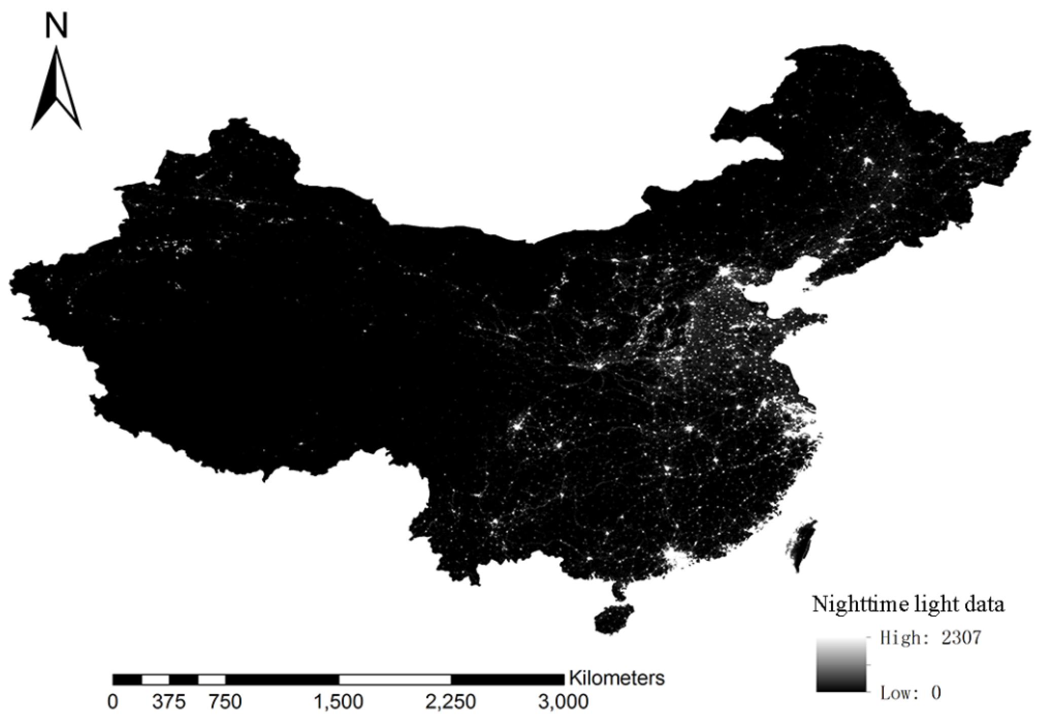
To explore the effect of the built-up environment on nighttime light, we should choose DMSP/OLS radiance-calibrated NTL data and GLAS waveform light detection and ranging (LiDAR) data in the same year. GLAS was only operated between 2003 and 2009. National Oceanic and Atmospheric Administration (NOAA) National Geophysical Data Center (NGDC) only published DMSP/OLS radiance-calibrated NTL data in 2004 and 2006, which coincided with the age of GLAS. Therefore, we choose NTL data and GLAS data in the most recent year (2006) to conduct this study. Therefore, DMSP/OLS radiance-calibrated NTL data with a spatial resolution of 30 arc seconds (about 1000 m) in 2006 were used in this study (Figure 1). These data are provided by NOAA NGDC (https://ngdc.noaa.gov/eog/dmsp/download_radcal.html). Ordinary DMSP/OLS NTL data have a very limited dynamic range, thus they could not accommodate bright sources (i.e., urban centers) [27,28]. To solve the saturation problem of ordinary DMSP/OLS NTL data, the NGDC produced a set of global NTL products with no sensor saturation based on the pre-flight sensor calibration. Radiance-calibrated NTL data is deemed to be unit-less because of lack of on-board calibration system for all DMSP/OLS. DMSP/OLS radiance-calibrated NTL data with a coordinate system of Geographic Latitude/longitude based on WGS 1984 were used in this study.

2.3. Land-Cover Data

GlobeLand30 data with a spatial resolution of 30 m have been used in this study. These data are obtained from the National Geomatics Center of China (NGCC) (http://www.globallandcover.com/GLC30Download/index.aspx). Only the GlobeLand30 data in 2000 and 2010 are available. The GlobeLand30 data in 2010 were selected in this study as their acquisition time is closer to 2006. The classification images used for data generation of GlobeLand30-2010 are mainly 30 m multispectral images, including Landsat Thematic Mapper (TM) and Enhanced Thematic Mapper + (ETM+) multispectral images and multispectral images of Chinese Environmental Disaster Alleviation Satellite (HJ-1). Ancillary datasets and reference materials, such as existing land-cover data and global fundamental geospatial data, were used to support sample selection, classifier training, and accuracy assessment. GlobeLand30-2010 data employ a 10-class land-cover classification scheme, namely cultivated land, forest, grassland, shrubland, wetland, water bodies, tundra, artificial surfaces, bareland, and permanent snow and ice. In this study, we mainly used the data of artificial surfaces and vegetation, including cultivated land, forest, grassland, and shrubland.

2.4. ICESat/GLAS Data

GLAS is a space-borne LiDAR instrument aboard the Ice, Cloud, and land Elevation Satellite (ICESat), and it was operated between 2003 and 2009. The GLAS laser sensor emitted laser pulses at a frequency of 40 Hz, with a wavelength of 1064 nm. The orbit altitude of the GLAS sensor was approximately 600 km and the repeat cycle was 183 days. In contrast to wall-to-wall observation, GLAS obtained individual footprint data, with a diameter of about 70 m and an interval of about 170 m along track. GLAS records the vertical structure of targets within each footprint, and from which the target height can be estimated.

GLAS data were provided by the National Snow and Ice Data Center (NSIDC) (http://nsidc.org/data/icesat/), and 15 data products (GLA01 ~ GLA15) can be acquired. GLA01 records raw waveform for each laser shot, which has 544 bins with the height interval of 0.15 m. GLA14 records the latitude, longitude, and elevation of each laser spot. In this study, GLA01 and GLA14 data of China in 2006 were used.

3. Methods

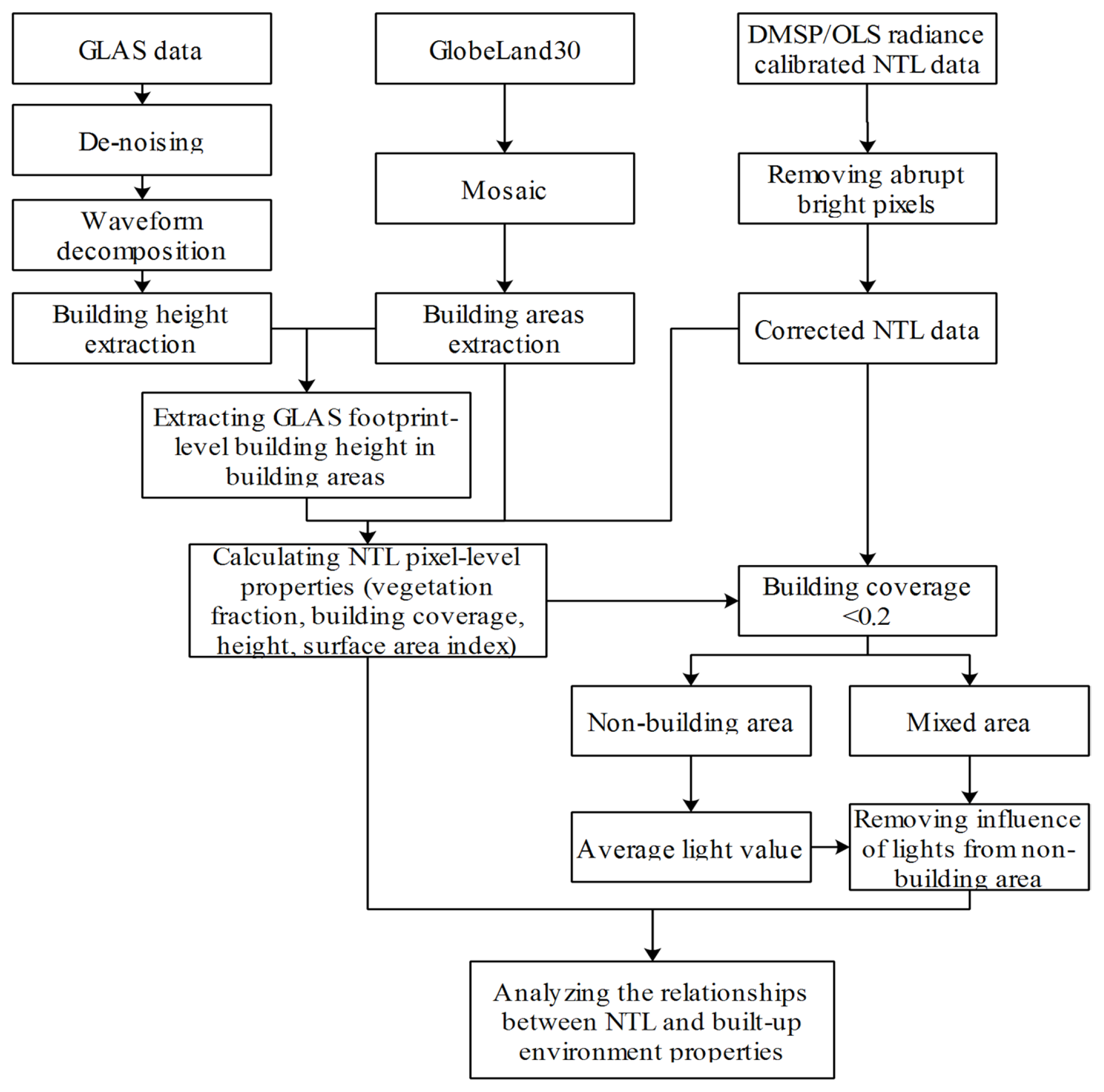
The technical flow chart of the methods used in this research is presented in Figure 2. This figure summarizes the steps of assessing the impact of built-up environment on nighttime lights. The five main procedures are GLAS data processing, NTL data correction, extraction of built-up environment properties, removal of the influence of lights from non-building areas, and analyses of the relationships between NTL and built-up environment properties.

3.1. GLAS Data Processing

Due to effects of atmosphere, clouds, and systematic noises, there are some noises in original GLAS waveform LiDAR data [29]. To obtain effective signals, low-pass digital Gauss filter was used to smooth the raw GLAS waveform data and reduce high-frequency noise at first [30]. Then mean background noise and the standard deviation of background noise were calculated from the first 20 and last 20 bins of waveform data [31]. The beginning and the end of signal were identified by the condition that signal was greater than three times the standard deviation of noise [32].

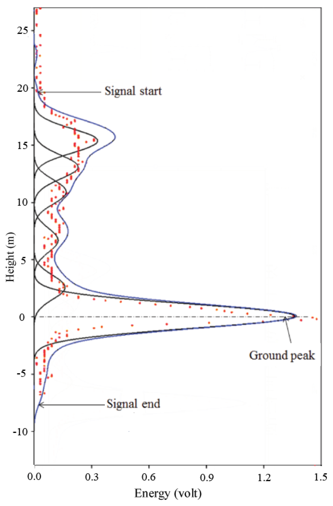
To extract height information of ground targets, Gaussian decomposition was conducted on GLAS waveform LiDAR data [33]. Each de-noised waveform was initially decomposed into multiple Gaussian functions. The initial parameters of Gaussian components, including amplitude, peak position, and standard deviation, were estimated at first, and then Levenberg-Marquardt (LM) algorithm was used to generate optimal Gaussian parameters [33]. An example of the result of Gaussian decomposition is shown in Figure 3. Several peak parameters, including peak position, peak amplitude, and peak width, were calculated from waveform data [31,34]. Assuming the last peak near ground is reflected from ground surfaces, the remaining peaks are reflected from targets [32,33]. Then the target height of each peak was calculated as height difference between the peak and ground peak. In the end, echo energy weighted height was calculated according to Equation (1), and it was used to represent average target height within the footprint:

$$BH={\displaystyle \sum _{i=1}^K{H}_i\cdot A_i}$$

(1)

where $BH$ is GLAS waveform data derived footprint-level building height, K is the number of Gaussian waveforms derived from Gaussian decomposition, $H_i$ the height of the ith Gaussian waveform, $A_i$ is the ratio of the area of the ith Gaussian waveform and whole area of GLAS waveform.

3.2. NTL Data Processing

There are some abrupt bright pixels in DMSP/OLS radiance-calibrated NTL data, which may be associated with oil fires oil in a refinery [35]. To address the issue of abrupt brightness, we employed a correction method according to Li et al. [36] and Shi et al. [35] in this study. Shanghai, Beijing, and Guangzhou are the three biggest and most developed cities of China. Theoretically, light-intensity values of the other regions should not exceed those three cities. We selected the maximum light-intensity value of these cities as the maximum value for all pixels in China. Then we identified the pixels whose light-intensity values were larger than the maximum value, and replaced them with the maximum values of their corrected second-order neighboring pixels. After the correction, light-intensity values of all pixels were less than or equal to the maximum light intensity.

3.3. Estimating Built-Up Environment Properties

To explore the effect of built-up environment on nighttime lights, several built-up environment properties are proposed to describe human settlements. Different ground features have different functions, so the distributions of ground features, which can be represented by building coverage and vegetation fraction, may affect nighttime lights to some degree. The intensity of nighttime light was determined by the number of lights exposed outside at night. Normally, lights are installed on every building floor, and building height is proportional to the number of floors, thus building height can determine the number of lights. Furthermore, building surface area seems to be more relevant to the number of lights exposed outside, so a new building surface-area index was also proposed and taken into account in this study.

All GlobeLand30 land-cover data were mosaicked to obtain the land-cover image of China by the mosaic module embedded in ArcGIS software. GlobeLand30 land-cover data consist of ten different land-cover types. Artificial surface represents building areas, while cultivated land, forest, grassland, and shrubland all represent vegetation growth areas, which are considered to be vegetation regions in this study. To estimate NTL pixel-level building coverage and vegetation fraction, the land-cover data and NTL data were overlaid first. Then, building coverage of each NTL pixel is calculated by dividing the number of building pixels by the total number of GlobeLand30 pixels within the NTL pixel (Equation (2)). A GlobeLand30 pixel belongs to the NTL pixel which contains most of it. Similarly, vegetation fraction of each NTL pixel is calculated by dividing the number of vegetation area pixels by the total number of pixels within the NTL pixel (Equation (3)).

$$Buildingcoverage=\frac{N_b}{N_t}$$

(2)

$$Vegetationfraction=\frac{N_g}{N_t}$$

(3)

where $N_b$ and $N_g$ represent the numbers of building pixels and vegetation pixels from GlobeLand30 image within the NTL pixel respectively, and $N_t$, represents the total number of GlobeLand30 pixels within the NTL pixel.

To obtain NTL pixel-level building height, all GLAS footprints were overlaid with the land-cover image of China first, and then GLAS footprints within building areas were extracted. GLAS data is recorded as individual footprint data with a diameter of about 70 m, while DMSP/OLS radiance-calibrated NTL data is recorded as wall-to-wall data with spatial resolution of about 1000 m (30 arc seconds). To match the NTL data and GLAS data which have different data recording modes for further analysis, all GLAS-derived footprint-level building height values within each NTL pixel were calculated using Equation (4).

$$Buildingheight=\frac{{\displaystyle \sum _{i=1}^{N}B{H}_i}}{N}$$

(4)

where $B{H}_i$ is footprint-level building height of the ith GLAS waveform within one NTL data pixel, N is the number of GLAS waveforms within one NTL pixel.

Surface-area index is the sum of all the building surface areas within the NTL pixel. Light cannot be exposed outside through penetrating the roof, so we did not consider roofs into the building surface areas in this study. Surface-area index is increasing with more lights exposed outside. Therefore, surface-area index can affect nighttime light intensity. In reality, only a few buildings are larger than 30 × 30 m. Thus, surface-area index can be approximated as the sum of average building surface area of each land-cover pixel within the NTL pixel, and its calculation method is shown in Equation (5).

$$Surfaceareaindex=4\cdot 30\cdot Buildingheight\cdot N_b$$

(5)

3.4. Removing Influence of Lights from Non-Building Areas

DMSP/OLS NTL data has a spatial resolution of about 1000 m. The pixel size is large enough to contain not only building areas but also non-building areas, such as parks and roads. Therefore, the lights from non-building areas, such as streetlights, also contributed to the light-intensity value of each NTL pixel. To analyze the relationship between NTL data and built-up environment properties more accurately, effects from non-building areas should be removed.

According to Chen et al. [37], we used a supervised method to remove light from non-building areas (Equation (6)). Firstly, we manually selected 250 pixels which contain no building areas with the help of high-resolution images from Google Earth [37]. Then, we counted the building coverage values of these pixels, and we found their building coverage were almost all lower than 0.2, which is consistent with previous studies [10]. Therefore, pixels with building coverage values lower than 0.2 were classified as non-building pixels, and the remaining pixels were classified as mixed pixels, which may still contain building and non-building areas. Finally, we calculated the average light intensity (ALI) of all non-building pixels based on Equation (7), and then we subtracted ALI from NTL value for each mixed pixel to remove non-building area effects for mixed pixels.

$$NTL=\{\begin{array}{l}NTL-ALI,ifBuildingcoverage\ge 0.2\\ NULL,ifBuildingcoverage<0.2\end{array}$$

(6)

$$ALI=\frac{{\displaystyle {\sum }_{i=1}^{N_{non-build}}NT{L}_i}}{N_{non-build}}$$

(7)

where $N_{non-build}$ is the number of pixels which was classified as non-building area, $NT{L}_i$ is the light intensity of the ith pixel in non-building area, ALI is average light intensity of all non-building areas.

4. Results

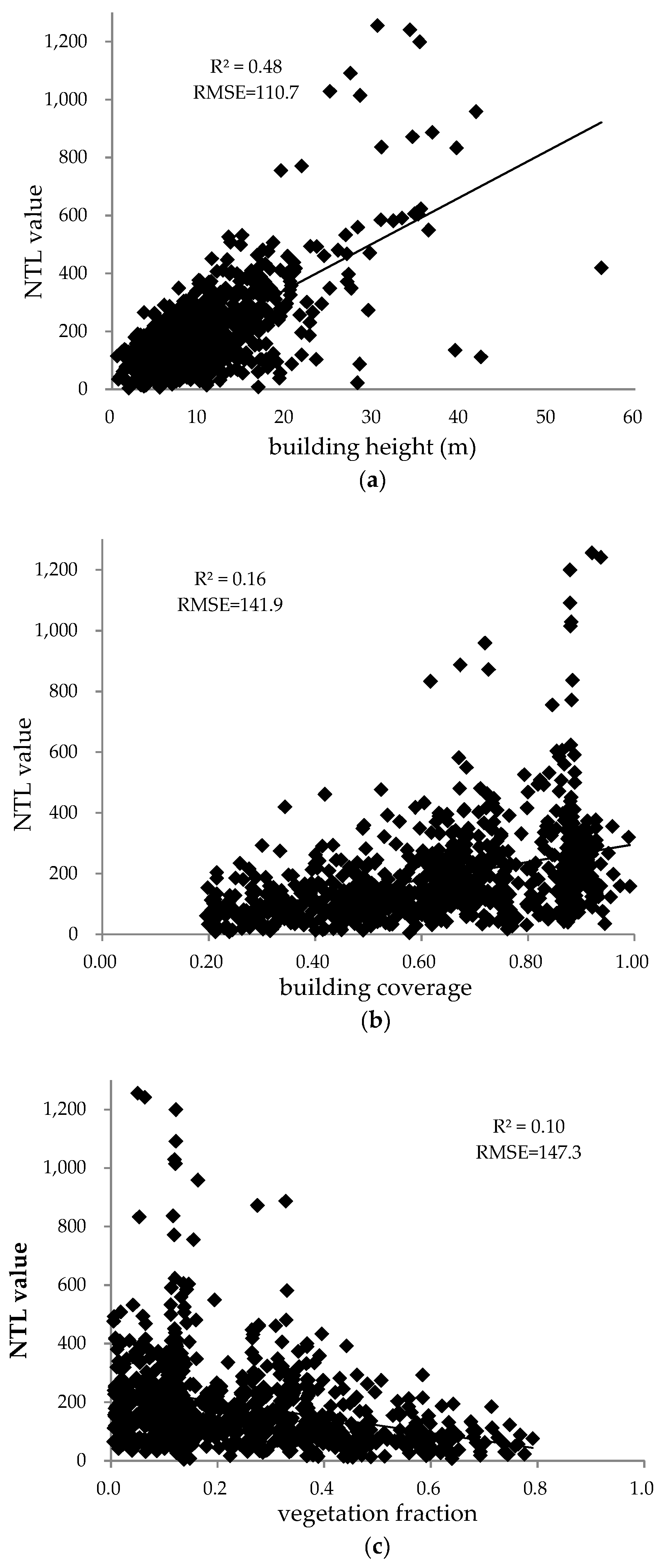
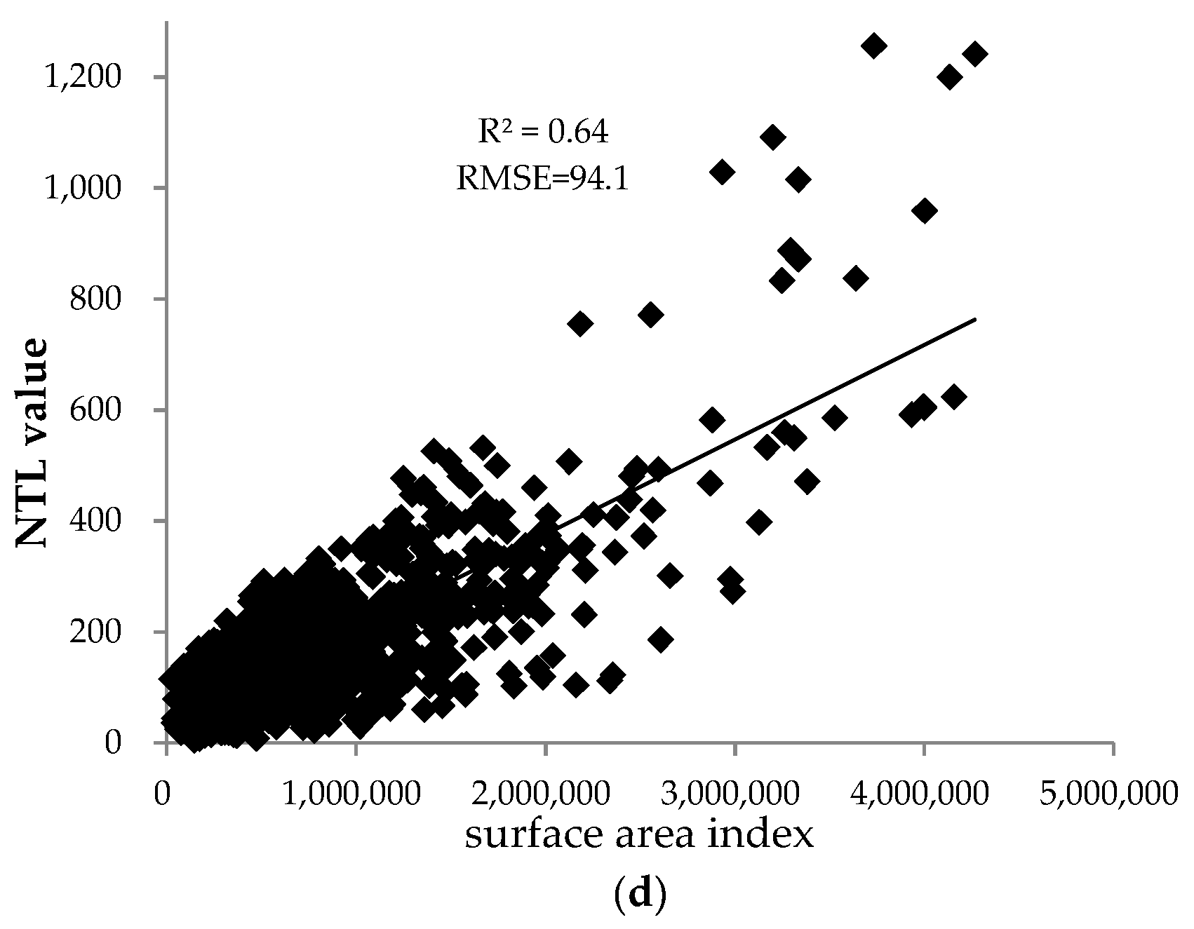
Linear regression analyses were conducted to examine the relationship between NTL data and each built-up environment property, i.e., building height, building coverage, vegetation fraction, and surface-area index. From the definition and calculation equation of surface-area index, we can see that surface-area index is a variable which combines the information of building height, building coverage, and vegetation fraction. Surface-area index is directly related to building height and building coverage, and it also indirectly related to vegetation fraction. Therefore, we did not run a multiple regression with all three explanatory variables in this study. The coefficient of determination (R²) and root-mean-square error (RMSE) were all calculated to assess the regression results. The scatter plots of DMSP/OLS radiance-calibrated NTL data and built-up environment properties are shown in Figure 4, together with R² values and RMSE values.

Figure 4a shows that radiance-calibrated NTL data ranges from 0 to 1300, and building height has a range of 0 m to 60 m. There is a moderately positive correlation between NTL data and building height, with the R² value of 0.48 and the RMSE value of 110.7. Figure 4b shows the correlation between building coverage and radiance-calibrated NTL data is positive and small, with the R² value of 0.16 and the RMSE value of 141.9. Vegetation fraction ranges from 0 to 1, and it has a weakly negative correlation with radiance-calibrated NTL data, with the R² value of 0.10 and the RMSE value of 147.3 (Figure 4c). Surface-area index has a range of 0 m to 35 m. The R² value of surface-area index and NTL data is 0.64, and the RMSE value of them is 94.1 (Figure 4d). Surface area index and radiance-calibrated NTL have the highest R² value, followed by building height and building coverage, and vegetation fraction has lowest R² value with radiance-calibrated NTL data. Meanwhile, vegetation fraction has the highest RMSE value with radiance-calibrated NTL, followed by building coverage and building height, and surface-area index has the lowest RMSE value with radiance-calibrated NTL data. Therefore, surface-area index has the highest correlation with NTL data, followed by building height and building coverage, and vegetation fraction has the lowest correlation with NTL data. In addition, surface-area index, building height, and building coverage all have positive correlation with NTL data, and only vegetation fraction has weak negative correlation with NTL data.

5. Discussion

5.1. Performance of Built-Up Environment Properties

Several limitations should be identified before discussing the performance of built-up environment properties. The first limitation is the time differences between GlobeLand30 land-cover data, GLAS waveform data, and DMSP/OLS radiance-calibrated NTL data. GLAS waveform data and NTL data were all acquired in 2006, while GlobeLand30 land-cover data were obtained in 2010. Due to urbanization, there are some changes in land cover between 2006 and 2010. However, the building areas in 2006 mostly remained the same as the building areas in 2010, so the accuracy of built-up environment properties would not be obviously affected. Another limitation is the small error caused by the trees around buildings. The trees within the GLAS footprint would affect LiDAR echo waveform, therefore they would affect the accuracy of building height slightly.

Building height showed a moderate and positive correlation to NTL data (R² = 0.48); i.e., as building height increased, NTL value increased (Figure 4a). Higher building height values correspond to more floors; therefore, they would contain more lights, which would lead to higher NTL value. These results were consistent with Kocifaj et al. [38], and they found total lumen output-normalized radiant intensity is depicted as a function of emission zenith angle for a set of building height values. For tall buildings, the light emissions directed upwards exceed the emissions to low elevation angles. Therefore, increasing building height results in an increase of NTL. However, building height also shapes light output pattern, meaning that the relative contribution of emissions to different angles changes as building height increases. This information is difficult to obtain from DMSP/OLS NTL data, so we cannot analyze the phenomenon clearly. Figure 4a showed that several points are below the regression line. This can be explained as although building height is high, there is only a small region within the NTL data pixel that is covered by buildings, so the number of lights is small, which leads to low NTL value. There are also several points obviously higher than the regression line in Figure 4a. This may be caused by large building coverage in these NTL data pixels.

Building coverage did not exhibit strong correlations with NTL data. Figure 4b showed a weak positive correlation between building coverage and NTL (R² = 0.16). Building coverage is the ratio of building area and total area within the NTL pixel, which demonstrates the coverage of buildings. Higher building coverage values mean that NTL pixel was more covered by buildings. According to Kocifaj et al. [38], the low correlation may be due to missing information on the light emissions to different zenith angle. Several points were obviously above the regression line, which might be caused by very high building heights. Figure 4b showed that although some points had high building coverage values, the NTL values were still very small, which might be caused by low building heights.

Vegetation fraction had a weak negative correlation with NTL, with R² of 0.10 (Figure 4c). Vegetation fraction is the ratio of vegetation area and total area within the NTL pixel, which demonstrates the coverage of vegetation. Higher vegetation fraction values mean that NTL pixel was more covered by vegetation, which would affect the intensity of nighttime light. These points, which obviously deviate from the regression line, may also be interpreted as very tall buildings. According to Kocifaj et al. [39], vegetation can reflect light from built-up elements, which implies flux emitted upward. Due to the chlorophyll concentration and vegetation nutrient change with season, the light-reflecting ability of vegetation also changes with season, which would cause seasonal NTL. Therefore, the correlation between NTL and vegetation fraction may show seasonal behavior. However, due to limited data sources, we cannot analyze the seasonal variation of the correlation between NTL and vegetation fraction in this study, which will need to be studied in the future.

Surface-area index correlated with NTL data strongly and positively, with the R² value of 0.64; i.e., as surface-area index increased, NTL value increased (Figure 4d). Surface-area index is a metric that corresponds to building surface area. Higher surface-area index values represent larger building surface area, so the light exposed outside would be more, which would result in higher NTL value. The correlation between NTL and surface-area index is stronger than the relationships between NTL and building height and between NTL and building coverage. This can be explained as the surface-area index containing both building height properties and the number of building pixels, which is related to building coverage properties, so it can describe human settlements more accurately, which would obviously affect the nighttime light intensity. Therefore, surface-area index has a better explanatory power for NTL value than other built-up environment properties.

5.2. Effects of Building Heights

Due to the differences in architectural styles and economic conditions, the building heights across China are diverse. According to the code for design of civil buildings in China, buildings below four floors are low-rise buildings, buildings between four floors to six floors are middle-level buildings, and buildings above six floors are high-rise buildings. The residential building module coordination standard of China indicated that single-floor height is about 2.8 m. Therefore, in this study, the maximum heights of the buildings within GLAS footprint smaller than 8.4 m are classified as low-rise buildings, the maximum height of the buildings between 8.4 m and 16.8 m are classified as middle-level buildings, and the maximum height of the buildings larger than 16.8 m are classified as high-rise buildings.

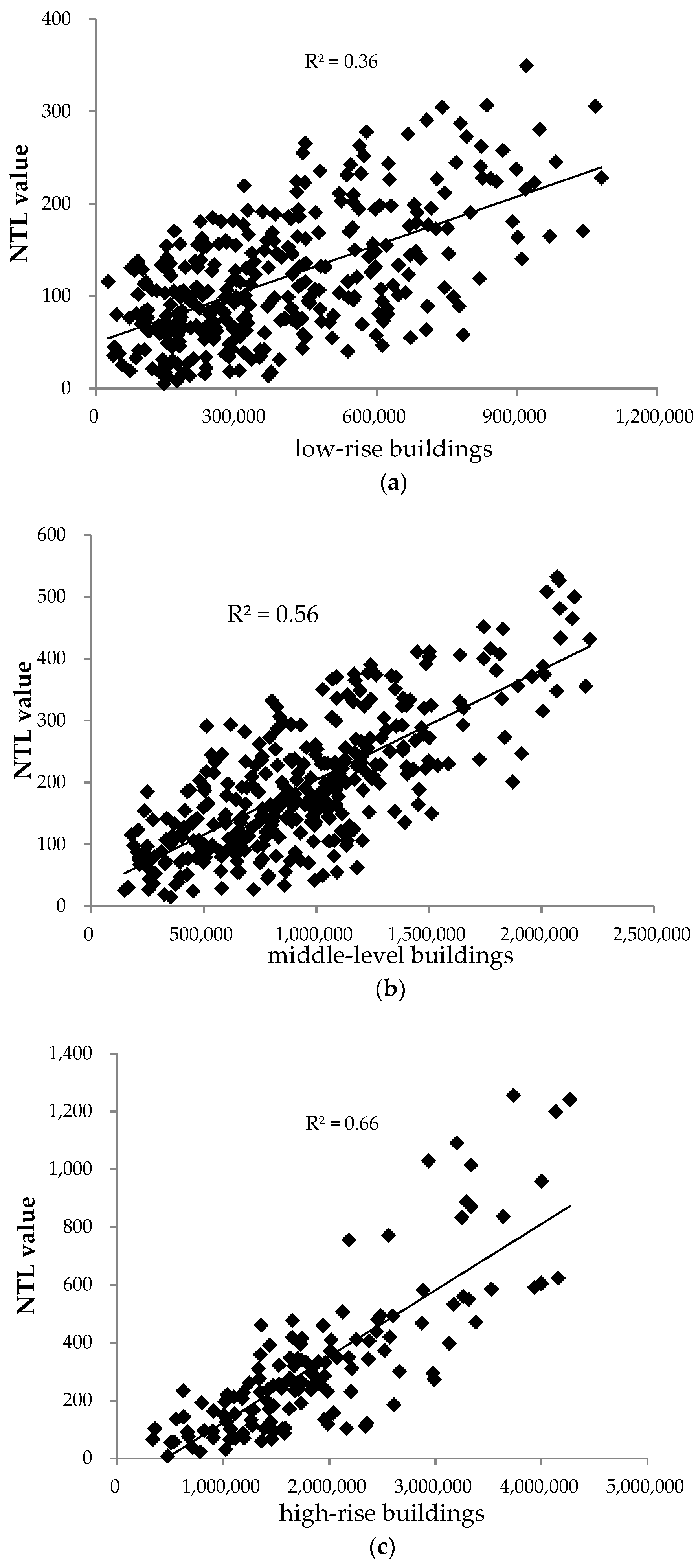
To explore whether building height would affect the relationship between radiance-calibrated NTL data and surface-area index, we conducted simple linear regressions between radiance-calibrated NTL data and surface-area index at different building heights, and the results are shown in Figure 5. Figure 5a shows that radiance-calibrated NTL data of low-rise buildings has a moderate positive correlation with surface-area index, with the R² value of 0.36. Figure 5b shows that the correlation between radiance-calibrated NTL data and surface-area index of middle-level buildings was positive and higher, with the R² value of 0.56. Radiance-calibrated NTL data and surface-area index of high-rise buildings is also positive, and the R² value was 0.66. Therefore, the correlation between radiance-calibrated NTL data and surface-area index of high-rise buildings is the highest, followed by middle-level buildings, and the correlation of low-rise buildings is the lowest. It can be concluded that building height affects NTL data, and the higher the building height, the stronger the correlation between NTL data and surface-area index. This can be explained by the fact that in some building areas with lower building heights, the trees around buildings may be higher than the buildings, which would lead to higher surface-area index estimation values than true values. In addition, due to the limitation of the statistical method used in Section 3.4, there are still some lights from non-building areas that cannot be removed when the values of non-building lights are very high.

5.3. Effects of Regional Economic Development Level

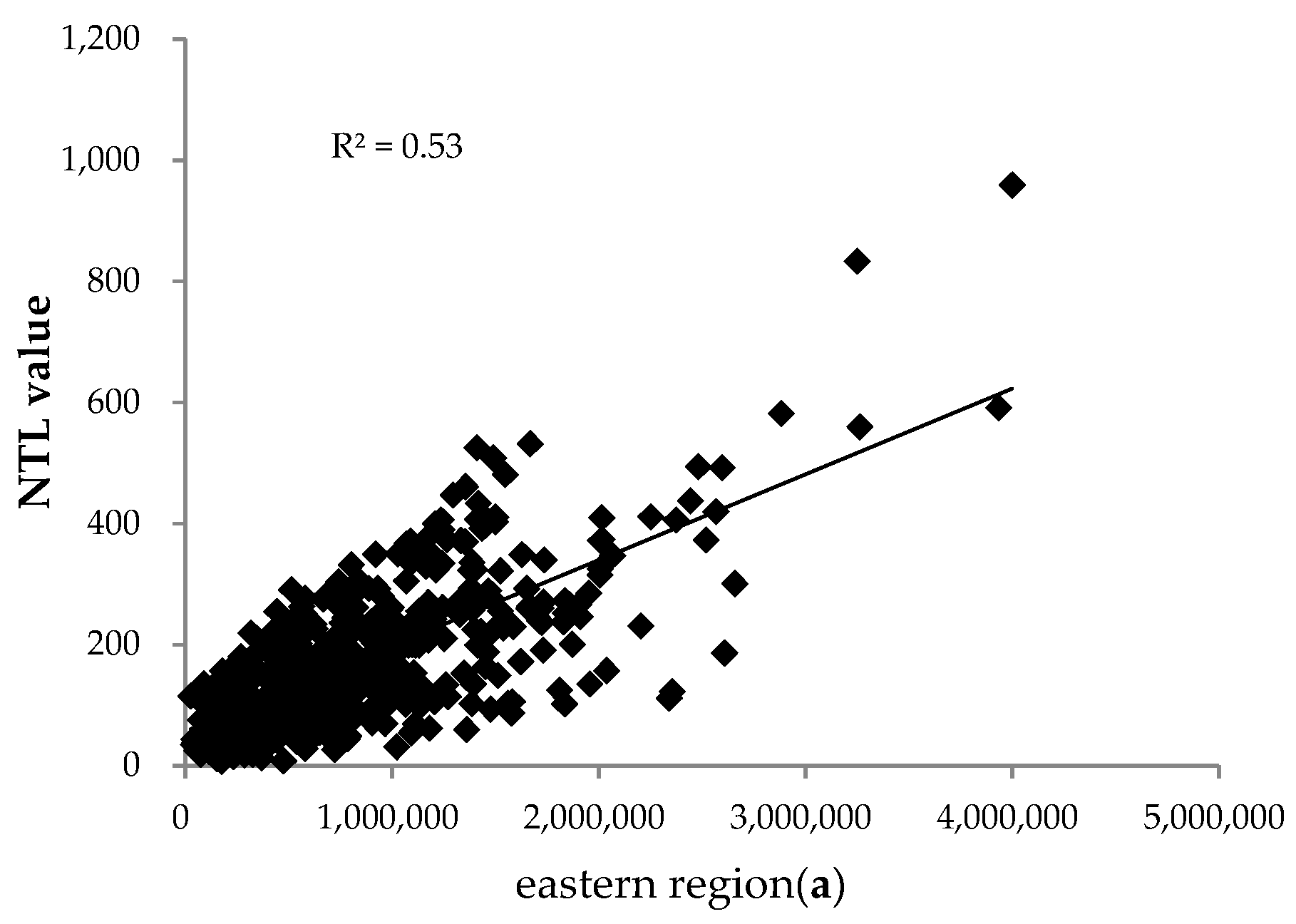
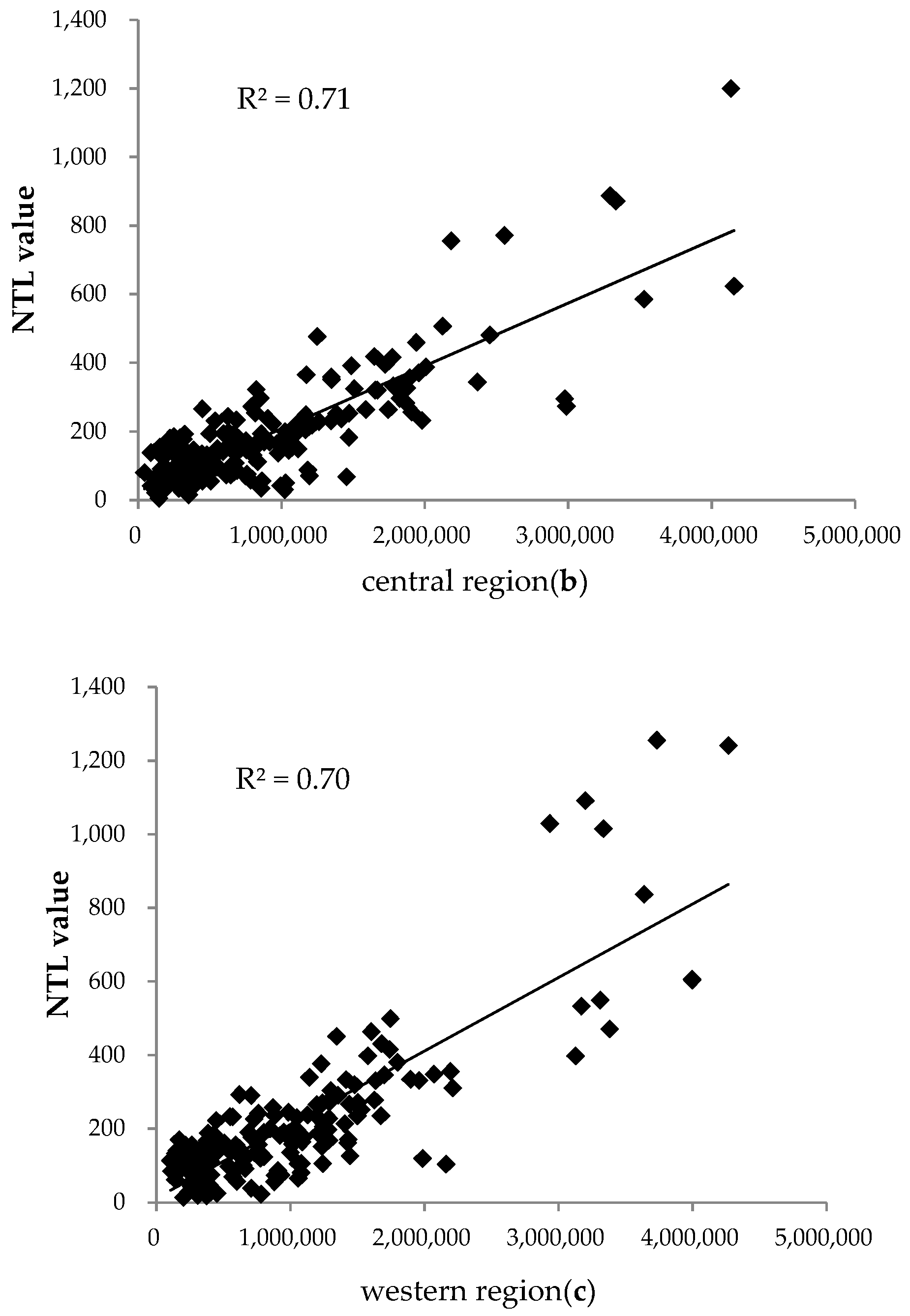
To investigate whether regional economic development level would affect the relationship between radiance-calibrated NTL data and surface-area index, we conducted linear regressions between NTL data and surface-area index of the three economic zones in China, and results are shown in Figure 6. Figure 6a showed that radiance-calibrated NTL data of China’s eastern region had a positive correlation with surface-area index, with the R² value of 0.53. Figure 6b showed that the correlation between radiance-calibrated NTL data and surface-area index of China’s central region was higher (R² = 0.71). Radiance-calibrated NTL data and surface-area index of China’s western region was also positive, and the R² value was 0.70. Therefore, the correlation between radiance-calibrated NTL data and surface-area index of the eastern region is the lowest, and the correlation of the central and western regions are all high. It can be concluded that regional economic development level affects nighttime lights, and when regional economic development level is high, the relationship between NTL data and surface-area index is relatively weak. This may be explained by the fact that China’s eastern region has a relatively developed economy, and the public lighting infrastructure is better. Therefore, there are more lights from non-building areas (such as streets and parks) in the eastern region of China, which cannot be completely removed by the statistical method used in Section 3.4. However, the central and western regions of China are economically underdeveloped areas. where the influences of non-building areas on NTL data are not obvious, and any such influences could have been removed in Section 3.4.

6. Conclusions

In this study, the effect of the built-up environment on nighttime light was investigated. Four NTL pixel-level built-up environment properties—building height, building coverage, vegetation fraction, and surface-area index—were proposed, and they were extracted from GLAS waveform LiDAR data, GlobeLand30 land-cover data, and DMSP/OLS radiance-calibrated NTL data. We also removed the influence of non-building area on nighttime lights. Statistical regression results showed that building coverage, building height, and surface-area index all had positive correlations with NTL data, while vegetation fraction had a negative correlation with NTL data. Surface-area index had the highest correlation with NTL data (R² = 0.64 and RMSE = 94.1), followed by building height (R² = 0.48 and RMSE = 110.7), and building coverage and vegetation fraction all had weak correlations with NTL data (R² < 0.2). Therefore, building height has a moderate impact on NTL, and surface-area index affects NTL significantly, because it is proportional to the number of lights exposed outside. Moreover, sensitivity analyses indicate that the relationship between nighttime lights and surface-area index is stronger with the increase of building height, and the correlation becomes relatively weak when regional economic development level is higher. Overall, these results make us identify the determinants of nighttime light clearly. Future research should consider whether the effect of built-up environment on nighttime light will be different or consistent in other years, other countries, and other scales.

References

- Li, X.; Ge, L.; Chen, X. Quantifying contribution of land use types to nighttime light using an unmixingmodel. IEEE Geosci. Remote Sens. Lett. 2014, 11, 1667–1771. [Google Scholar] [CrossRef]
- Elvidge, C.D.; Imhoff, M.L.; Baugh, K.E.; Hobson, V.R.; Nelson, I.; Safran, J.; Dietz, J.B.; Tuttle, B.T. Night-time lights of the world: 1994–1995. ISPRS J. Photogramm. 2001, 56, 81–99. [Google Scholar] [CrossRef]
- Elvidge, C.D.; Safran, J.; Tuttle, B.; Sutton, P.; Cinzano, P.; Pettit, D.; Arvesen, J.; Small, C. Potential for global mapping of development via a nightsat mission. GeoJournal 2007, 69, 45–53. [Google Scholar] [CrossRef]
- Raupach, M.R.; Rayner, P.J.; Paget, M. Regional variations in spatial structure of nightlights, population density and fossil-fuel co2 emissions. Energy Policy 2010, 38, 4756–4764. [Google Scholar] [CrossRef]
- Ma, T.; Zhou, Y.; Zhou, C.; Haynie, S.; Pei, T.; Xu, T. Night-time light derived estimation of spatio-temporal characteristics of urbanization dynamics using dmsp/ols satellite data. Remote Sens. Environ. 2015, 158, 453–464. [Google Scholar] [CrossRef]
- Elvidge, C.D.; Baugh, K.E.; Kihn, E.A.; Kroehl, H.W.; Davis, E.R. Mapping city lights with nighttime data from the dmsp operational linescan system. Photogramm. Eng. Remote Sens. 1997, 63, 727–734. [Google Scholar]
- Elvidge, C.D.; Baugh, K.E.; Kihn, E.A.; Kroehl, H.W.; Davis, E.R.; Davis, C.W. Relation between satellite observed visible-near infrared emissions, population, economic activity and electric power consumption. Int. J. Remote Sens. 2010, 18, 1373–1379. [Google Scholar] [CrossRef]
- Elvidge, C.D.; Sutton, P.C.; Ghosh, T.; Tuttle, B.T.; Baugh, K.E.; Bhaduri, B.; Bright, E. A global poverty map derived from satellite data. Comput. Geosci. 2009, 35, 1652–1660. [Google Scholar] [CrossRef]
- Elvidge, C.D.; Ziskin, D.; Baugh, K.E.; Tuttle, B.T.; Ghosh, T.; Pack, D.W.; Erwin, E.H.; Zhizhin, M. A fifteen year record of global natural gas flaring derived from satellite data. Energies 2009, 2, 595–622. [Google Scholar] [CrossRef]
- Zhou, Y.; Smith, S.J.; Elvidge, C.D.; Zhao, K.; Thomson, A.; Imhoff, M. A cluster-based method to map urban area from dmsp/ols nightlights. Remote Sens. Environ. 2014, 147, 173–185. [Google Scholar] [CrossRef]
- Amaral, S.; Monteiro, A.M.V.; Camara, G.; Quintanilha, J.A. Dmsp/ols night-time light imagery for urban population estimates in the brazilian amazon. Int. J. Remote Sens. 2006, 27, 855–870. [Google Scholar] [CrossRef]
- Bhandari, L.; Roychowdhury, K. Night lights and economic activity in india: A study using dmsp-ols night time images. Proc. Asia Pac. Adv. Netw. 2011, 32, 218. [Google Scholar] [CrossRef]
- Wang, W.; Cheng, H.; Zhang, L. Poverty assessment using dmsp/ols night-time light satellite imagery at a provincial scale in china. Adv. Space Res. 2012, 49, 1253–1264. [Google Scholar] [CrossRef]
- Kuechly, H.U.; Kyba, C.C.; Ruhtz, T.; Lindemann, C.; Wolter, C.; Fischer, J.; Hölker, F. Aerial survey and spatial analysis of sources of light pollution in berlin, germany. Remote Sens. Environ. 2012, 126, 39–50. [Google Scholar] [CrossRef]
- Katz, Y.; Levin, N. Quantifying urban light pollution—A comparison between field measurements and eros-b imagery. Remote Sens. Environ. 2016, 177, 65–77. [Google Scholar] [CrossRef]
- Falchi, F.; Cinzano, P.; Elvidge, C.D.; Keith, D.M.; Haim, A. Limiting the impact of light pollution on human health, environment and stellar visibility. J. Environ. Manag. 2011, 92, 2714–2722. [Google Scholar] [CrossRef]
- Bauer, S.E.; Wagner, S.E.; Burch, J.; Bayakly, R.; Vena, J.E. A case-referent study: Light at night and breast cancer risk in georgia. Int. J. Health Geogr. 2013, 12, 23. [Google Scholar] [CrossRef]
- Miller, M.W. Apparent effects of light pollution on singing behavior of american robins. Condor 2006, 108, 130–139. [Google Scholar] [CrossRef]
- Cinzano, P.; Falchi, F.; Elvidge, C.D. The first world atlas of the artificial night sky brightness. Mon. Not. R. Astron. Soc. 2001, 328, 689–707. [Google Scholar] [CrossRef]
- Imhoff, M.L.; Lawrence, W.T.; Elvidge, C.D.; Paul, T.; Levine, E.; Privalsky, M.V.; Brown, V. Using nighttime dmsp/ols images of city lights to estimate the impact of urban land use on soil resources in the united states. Remote Sens. Environ. 1997, 59, 105–117. [Google Scholar] [CrossRef]
- Levin, N.; Zhang, Q. A global analysis of factors controlling viirs nighttime light levels from densely populated areas. Remote Sens. Environ. 2017, 190, 366–382. [Google Scholar] [CrossRef]
- Levin, N. The impact of seasonal changes on observed nighttime brightness from 2014 to 2015 monthly viirs dnb composites. Remote Sens. Environ. 2017, 193, 150–164. [Google Scholar] [CrossRef]
- Levin, N.; Johansen, K.; Hacker, J.M.; Phinn, S. A new source for high spatial resolution night time images—The eros-b commercial satellite. Remote Sens. Environ. 2014, 149, 1–12. [Google Scholar] [CrossRef]
- Cheng, F.; Wang, C.; Wang, J.; Tang, F.; Xi, X. Trend analysis of building height and total floor space in beijing, china using icesat/glas data. Int. J. Remote Sens. 2011, 32, 8823–8835. [Google Scholar] [CrossRef]
- Gong, P.; Li, Z.; Huang, H.; Sun, G.; Wang, L. ICEsat GLAS data for urban environment monitoring. IEEE Trans. Geosci. Remote Sens. 2011, 49, 1158–1172. [Google Scholar] [CrossRef]
- Yu, B.; Shu, S.; Liu, H.; Song, W.; Wu, J.; Wang, L.; Chen, Z. Object-based spatial cluster analysis of urban landscape pattern using nighttime light satellite images: A case study of china. Int. J. Geogr. Inf. Sci. 2014, 28, 2328–2355. [Google Scholar] [CrossRef]
- Letu, H.; Hara, M.; Yagi, H.; Naoki, K.; Tana, G.; Nishio, F.; Shuhei, O. Estimating energy consumption from night-time dmps/ols imagery after correcting for saturation effects. Int. J. Remote Sens. 2010, 31, 4443–4458. [Google Scholar] [CrossRef]
- Elvidge, C.D.; Baugh, K.E.; Dietz, J.B.; Bland, T.; Sutton, P.C.; Kroehl, H.W. Radiance calibration of dmsp-ols low-light imaging data of human settlements. Remote Sens. Environ. 1999, 68, 77–88. [Google Scholar] [CrossRef]
- Xing, Y.; Qiu, S.; Ding, J.; Tian, J. Estimation of regional forest aboveground biomass combining icesat-glas waveforms and hj-1a/hsi hyperspectral imageries. ISPRS Int. Arch. Photogramm. Remote Sens. Spat. Inf. Sci. 2016, 41, 731–737. [Google Scholar] [CrossRef]
- Fang, Z.; Cao, C.; Ji, W.; Xu, M.; Chen, W. Study on forest aboveground biomass synergy inversion from glas and hj-1 data. Proc. SPIE 2012, 8524. [Google Scholar]
- Yu, Y.; Yang, X.; Fan, W. Estimates of forest structure parameters from glas data and multi-angle imaging spectrometer data. Int. J. Appl. Earth Obs. Geoinf. 2015, 38, 65–71. [Google Scholar] [CrossRef]
- Sun, G.; Ranson, K.J.; Kimes, D.S.; Blair, J.B.; Kovacs, K. Forest vertical structure from glas: An evaluation using lvis and srtm data. Remote Sens. Environ. 2008, 112, 107–117. [Google Scholar] [CrossRef]
- Luo, S.; Wang, C.; Li, G.; Xi, X. Retrieving leaf area index using icesat/glas full-waveform data. Remote Sens. Lett. 2013, 4, 745–753. [Google Scholar] [CrossRef]
- Harding, D.J. ICESat waveform measurements of within-footprint topographic relief and vegetation vertical structure. Geophys. Res. Lett. 2005, 32. [Google Scholar] [CrossRef] [Green Version]
- Shi, K.; Yu, B.; Huang, Y.; Hu, Y.; Yin, B.; Chen, Z.; Chen, L.; Wu, J. Evaluating the ability of npp-viirs nighttime light data to estimate the gross domestic product and the electric power consumption of china at multiple scales: A comparison with dmsp-ols data. Remote Sens. 2014, 6, 1705–1724. [Google Scholar] [CrossRef]
- Li, Q.; Lu, L.; Weng, Q.; Xie, Y.; Guo, H. Monitoring urban dynamics in the southeast U.S.A. Using time-series dmsp/ols nightlight imagery. Remote Sens. 2016, 8, 578. [Google Scholar] [CrossRef]
- Chen, Z.; Yu, B.; Hu, Y.; Huang, C.; Shi, K.; Wu, J. Estimating house vacancy rate in metropolitan areas using npp-viirs nighttime light composite data. IEEE J. STARS 2015, 8, 2188–2197. [Google Scholar] [CrossRef]
- Kocifaj, M. Towards a comprehensive city emission function (ccef). J. Quant. Spectrosc. RA 2018, 205, 253–266. [Google Scholar] [CrossRef]
- Kocifaj, M.; Solano-Lamphar, H.A.; Videend, G. Night-sky radiometry can revolutionize the characterization of light-pollution sources globally. Proc. Natl. Acad. Sci. USA 2019, 116, 7712–7717. [Google Scholar] [CrossRef] [Green Version]
Figure 1.
Spatial distribution of DMSP/OLS radiance-calibrated NTL data of mainland China in 2006.
Figure 2.
Technical flow chart of the methods used in this research.
Figure 3.
An example of raw GLAS waveform (red dots), Gaussian fitting (blue line), and decomposed Gaussian components (black line).
Figure 4.
Correlations between DMSP/OLS radiance-calibrated NTL data and built-up environment properties: (a) building height; (b) building coverage; (c) vegetation fraction; (d) surface-area index.
Figure 5.
Correlations between DMSP/OLS radiance-calibrated NTL data and surface-area index of (a) low-rise buildings, (b) middle-level buildings, and (c) high-rise buildings.
Figure 6.
Correlations between DMSP/OLS radiance-calibrated NTL data and surface-area index of the three economic zones of China: (a) eastern region, (b) central region, and (c) western region.
© 2019 by the authors. Licensee MDPI, Basel, Switzerland. This article is an open access article distributed under the terms and conditions of the Creative Commons Attribution (CC BY) license (http://creativecommons.org/licenses/by/4.0/).
Share and Cite
MDPI and ACS Style
Wang, C.; Qin, H.; Zhao, K.; Dong, P.; Yang, X.; Zhou, G.; Xi, X. Assessing the Impact of the Built-Up Environment on Nighttime Lights in China. Remote Sens. 2019, 11, 1712. https://0-doi-org.brum.beds.ac.uk/10.3390/rs11141712
AMA Style
Wang C, Qin H, Zhao K, Dong P, Yang X, Zhou G, Xi X. Assessing the Impact of the Built-Up Environment on Nighttime Lights in China. Remote Sensing. 2019; 11(14):1712. https://0-doi-org.brum.beds.ac.uk/10.3390/rs11141712
Chicago/Turabian StyleWang, Cheng, Haiming Qin, Kaiguang Zhao, Pinliang Dong, Xuebo Yang, Guoqing Zhou, and Xiaohuan Xi. 2019. "Assessing the Impact of the Built-Up Environment on Nighttime Lights in China" Remote Sensing 11, no. 14: 1712. https://0-doi-org.brum.beds.ac.uk/10.3390/rs11141712
Note that from the first issue of 2016, this journal uses article numbers instead of page numbers. See further details here.