Dasymetric Mapping Using UAV High Resolution 3D Data within Urban Areas


Interdisciplinary Centre of Social Sciences (CICS.NOVA), Faculty of Social Sciences and Humanities, (NOVA FCSH), Universidade NOVA de Lisboa, Av. de Berna, 26-C, 1069-061 Lisboa, Portugal
*
Author to whom correspondence should be addressed.
Remote Sens. 2019, 11(14), 1716; https://0-doi-org.brum.beds.ac.uk/10.3390/rs11141716
Submission received: 29 May 2019
/
Revised: 4 July 2019
/
Accepted: 13 July 2019
/
Published: 19 July 2019
(This article belongs to the Special Issue Remote Sensing for Urban Morphology)
Abstract
:Multi-temporal analysis of census small-area microdata is hampered by the fact that census tract shapes do not often coincide between census exercises. Dasymetric mapping techniques provide a workaround that is nonetheless highly dependent on the quality of ancillary data. The objectives of this work are to: (1) Compare the use of three spatial techniques for the estimation of population according to census tracts: Areal interpolation and dasymetric mapping using control data—building block area (2D) and volume (3D); (2) demonstrate the potential of unmanned aerial vehicle (UAV) technology for the acquisition of control data; (3) perform a sensitivity analysis using Monte Carlo simulations showing the effect of changes in building block volume (3D information) in population estimates. The control data were extracted by a (semi)-automatic solution—3DEBP (3D extraction building parameters) developed using free open source software (FOSS) tools. The results highlight the relevance of 3D for the dasymetric mapping exercise, especially if the variations in height between building blocks are significant. Using low-cost UAV backed systems with a FOSS-only computing framework also proved to be a competent solution with a large scope of potential applications.
1. Introduction
In the urban planning of small areas, their characterization and analysis precedes the drafting of intervention proposals. The aforementioned urban analysis requires updated information, both for the spatial distribution of the population and for residential buildings. This is a common practice of urban planners and urbanists. For this characterization and analysis, census data are used. These census data are only useful for urban planning if they have a large spatial disaggregation. Therefore, they have to be collected by urban area units of a dimension that enables large-scale urban planning (census tracts). However, the geometry of these census tracts has been found to change between two censuses, either by spatial aggregation or by spatial disaggregation. This aggregation or spatial disintegration occurs especially when new structures are built or when urban densification processes occur. Now, these tract boundary changes imply that the population has to be recalculated at time t0 so we can compare it with time t1, …, tn. After recalculating the population, urban planners and urbanists can perceive the evolution of the population in these urban areas. This evolution of the population is particularly useful to study enclosures, lost spaces, public spaces, proximity, contiguity and urban density [1]. Thus, in this context, dasymetric mapping using different geometrical schemes and different types of information becomes useful [2,3,4].
The use of different geometrical schemes (zones) to aggregate geographical data into polygons has long been recognized as problematic [5,6]. There are issues related to the assumption of stationarity inside each spatial unit; this is commonly known as an ecological fallacy [7]. Related but not the same is that different aggregation geometries result in the well-documented modifiable areal unit problem—MAUP [8], which hampers the multi-temporality of multivariate analysis. General purpose solutions involve the use of dasymetric mapping techniques, in which data is re-allocated and aggregated according to a common geometry [5].
Spatial interpolation techniques, in particular dasymetric mapping, allow the re-allocation of areal data from source to target zones/geometries. In the present work, the terms “geometrical schemes” or simply “geometry (or geometries)” are used instead of “zones”, “areas”, “regions” or simply “polygons”. Although they are considered more general, it must be clear that the object of this work is only data aggregated into polygons. The efficiency of a dasymetric mapping exercise strongly depends on the quality of the ancillary (or control) data, which allows you to drop the intra-regional isotropy assumption, in other words, spatial variation of the variable of interest is not assumed to follow a homogeneous distribution within each spatial unit. Examples of ancillary or control datasets are land-use patterns or building footprints. Studies that use different methodologies may be grouped following the classification used in [6]. Areal interpolation exercises may take into account one (or more) of the following spatial attributes: Form, structure and function. The first takes into account the scale and shape of the source and target geometries; the second—structure—is related to local variation according to some homogeneous geographical layer (e.g., building footprints); finally, function allows the stratification of ancillary data considering a certain attribute (e.g., distinction between residential and commercial buildings).
The dasymetric mapping is essential for the multi-temporal analysis of census datasets, when the shapes of the census tracts do not coincide [9]. The application of dasymetric mapping for the estimation of population size can be improved by using ancillary 2D or 3D data related to the buildings. Currently the acquisition of 2D/3D data from census areas is easier to obtain and it is faster and cheaper than using classical topography and photogrammetry surveying methods. In this work, the 2D/3D data obtained from a low-cost technology allowed us to look at the structure of census tracts.
Advances in digital photogrammetry, airborne sensor systems (imaging or laser) and computer vision have turned the acquisition of 2D/3D geographical data into a more time- and cost-effective process, based on a high level of automation. Furthermore, the development of unmanned aerial vehicles (UAV) systems has enabled the production of photogrammetric survey data with relative ease [10,11].
Generically, a UAV system is a low-cost user-friendly technology, which offers great potential and support in various applications [12], such as 3D building modeling for urban and spatial planning [13,14], particularly in areas where no other source of volumetric information exists or when it does exist it is not updated. This technology can also enable the fast acquisition of 2D/3D data, with the positional accuracy of centimeters required for the estimation of building parameters [13].
The two major types of UAV aircrafts are fixed-wings and multi-rotors. Fixed-wing UAVs are more stable than multi-rotors [15], however they require a larger take-off and landing area. On the other hand, they are more suited to acquire urban objects for modeling purposes than the other type of UAVs. In this work, a fixed-wing system—Swinglet CAM—produced by SenseFly was used for the acquisition of a 3D point cloud over the study area. This is one of the most lightweight systems (weighing around 500 g), which enables the performance of a fast survey at low altitude [16].
A UAV system integrates a miniaturized direct georeferencing system [17] and a small sensor (RGB, CIR, etc.), which together allow the acquisition of georeferenced image pairs. The direct georeferencing system allows a “real-time georeferencing” [18] through a positioning system based on GNSS (global navigation satellite systems) and an inertial measurement unit (IMU). The GNSS provides the position of the laser sensor (X0, Y0, Z0) based on one or more GNSS base stations and the IMU provides the sensor’s attitude and heading angles (roll around x-axis, pitch around y-axis and yaw around z-axis). The weakness of this technology is its flight autonomy (battery life is usually 30 min), thus it is used only for small areas.
Furthermore, the advances in the development of robust computational algorithms have allowed the production of high-density 3D point clouds with dozens of points per square meter from a dense image matching of multiple image pairs [19]. This processing of image pairs is a combination of computer vision and photogrammetric techniques [20], which comprise the image matching of image pairs and the external orientation based on the adjustment of the six parameters (X0, Y0, Z0, roll, pitch, yaw) obtained from direct georeferencing. In general, a high-density 3D point cloud is obtained from high-resolution images with very high forward (along the flight direction) and lateral (between flight lines) overlap of about 90% and 60%, respectively.
The use of a large volume of data as a 3D point cloud for the (semi)-automatic extraction of building parameters requires the development of robust methodologies that need to be optimized or updated in order to allow different study-areas to be used. The use of 3D point clouds in the extraction of building parameters has been demonstrated by [13,14]. 3D data extracted from satellite imagery [21] and LiDAR [22] have also already been used as auxiliary information in dasymetric exercises.
This work estimates population size in 2001 according to the 2011 census tracts for a residential building area of interest. Data from the 2001 census is re-allocated according to the 2011 census tracts spatial aggregation scheme using three different techniques: (i) Taking into account the area of each census tract, and assuming intra-regional stationarity, data is interpolated from source to target geometries; (ii) using building block footprints as control data, the isotropy assumption is dropped and a dasymetric exercise is performed; and (iii) 3D data (height and volume) of building blocks is used to bring the exercise closer to reality. The area, height and volume of building blocks are extracted from the UAV imagery using the 3DEBP (3D extraction building parameters) methodology [23]. This work is innovative in the use of rough point cloud datasets to extract volumetric information as control data in a dasymetric mapping exercise. Primary data is obtained using low-cost UAV technologies. Furthermore, for this purpose, a methodology was developed using free open source software (FOSS) tools (excluding the acquisition of a 3D point cloud), which facilitate reproduction of the results, increases accountability, and reduces costs. The potential use of the same methodology with much larger datasets enables the large-scale computation of multi-temporal social-economic datasets.
Finally, in order to test the effect of variations in building volume, a sensitivity analysis was performed, allowing building block height to vary in existing buildings and the effect of taking into account missing elements (e.g., new buildings). Monte Carlo results demonstrate that the data quality of ancillary data is of paramount importance.
During this research, every software tool used for the development of methodology, described below, is FOSS [24] and the geo-demographic data used are freely available on the web [25]. These two elements permit reproducibility and follow recent trends towards a greater use of FOSS tools and free data dissemination [26].
2. Data and Methodology
The re-allocation of geographical data that characterize or are aggregated into areas (polygons) involves the creation of some sort of weighting scheme that can carry a proportion of the variable of interest from source to target spatial entities. For variable X, which is geographically distributed according to a certain source spatial scheme, its values are given by the set . The values of the same variable, according to the target scheme, are given by . Each value of X aggregated in T spatial units is given by the expression:
where k is the subset of n whose intersection with is not empty and is the proportion of , which is to be allocated to i.
In the case of two polygons, one from the source () and the other from the target geographical scheme (T), only the proportion of S, defined by , is going to be allocated to T. The re-allocation exercise, as mentioned, may be performed simply according to the area/size of each intersecting zone or using control datasets. The use of control datasets means that is allocated to taking into account the proportion of the weighting scheme based on 2D information (e.g., area of residential buildings) or 3D information (e.g., building volume).
2.1. Study-Area and Data
The study-area corresponds to a small neighborhood in the outskirts of Lisbon, with an extension of 150 m wide North to South and 600 m long East to West (Figure 1). It contains seven residential building blocks with tiled roofs, heterogeneous shapes and small differences in their overall height—the number of stories varies between four and six. This is a residential building area of interest containing a sample of buildings with the usual shape and design in the Lisbon metropolitan area. Therefore, this study-area contains representative residential buildings for the case of dasymetric mapping. The characteristics of the chosen neighborhood enabled the distinction of three types of building blocks (Figure 1): a. Regular (Zone A), b. irregular (Zone B) and c. building block islands (Zone C).
The objective was to estimate the population in 2001 according to the 2011 geometries (Figure 2), so the areal interpolation and dasymetric mapping exercises were used as source geometry (zones) census tracts (S) from 2001 and as target geometry census tracts (T) from 2011. In Portugal, census tract geometries are known as the Geographic Base for Information Referencing—BGRI (Figure 2).
For the analysis of results, geographical zones were classified from source and target schemes, as illustrated in Figure 2, according to the three zones A, B and C (Figure 1).
The re-allocation of 2001 census to the 2011 census tract shapes using control data (residential building block area and volume) required the acquisition of geographical data. These data were obtained from the processing of a UAV point cloud.
At the end of the summer of 2012, a UAV flight was performed on this residential area with a Swinglet CAM. This is one of the most lightweight systems, which enables a fast survey at low altitude over small urban areas without any human intervention during the flight. The study area was covered by 85 stereo aerial images (3000 by 4000 pixels each image). These aerial images were acquired (Figure 3) with a higher overlapping between them, which is about 80% along flight and 60% side overlap. The flight height average (above ground level) was 100 m over the study area, providing a ground sample distance (cm/pixel) of about 6 cm for imagery.
The UAV point cloud was obtained by an automatic processing workflow implemented in PIX4D. The georeferencing of every stereo pair was refined through the measuring of eight ground control points for every image where they appeared in order to obtain a more accurate point cloud [27]. Next, the 3D point cloud was automatically obtained through the multi-stereo image matching processing, which allows you to estimate a set of 3D points from the correlation between stereo pair pixels.
The result was more than one million points of the 3D point cloud, an average of around 11 points per square meter, which means that the average distance between points is about 30 cm.
Furthermore, the reference dataset obtained through classical photogrammetric restitution was used to benchmark area and height building parameters extracted from UAV point cloud. These reference datasets were 2D/3D accurate vector data (at a scale of 1:2000): Building footprints and elevations of each building (roof and terrain), produced between 2010 and 2011.
In addition, working with this small urban area (containing distinct shapes in terms of building footprints) was important for: (a) The development of a methodology that is independent from any performance tools; and (b) the study of the performance of a sensitivity analysis with great control over the effect of changing parameters.
2.2. Methodology
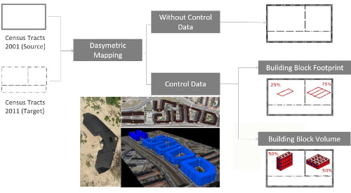
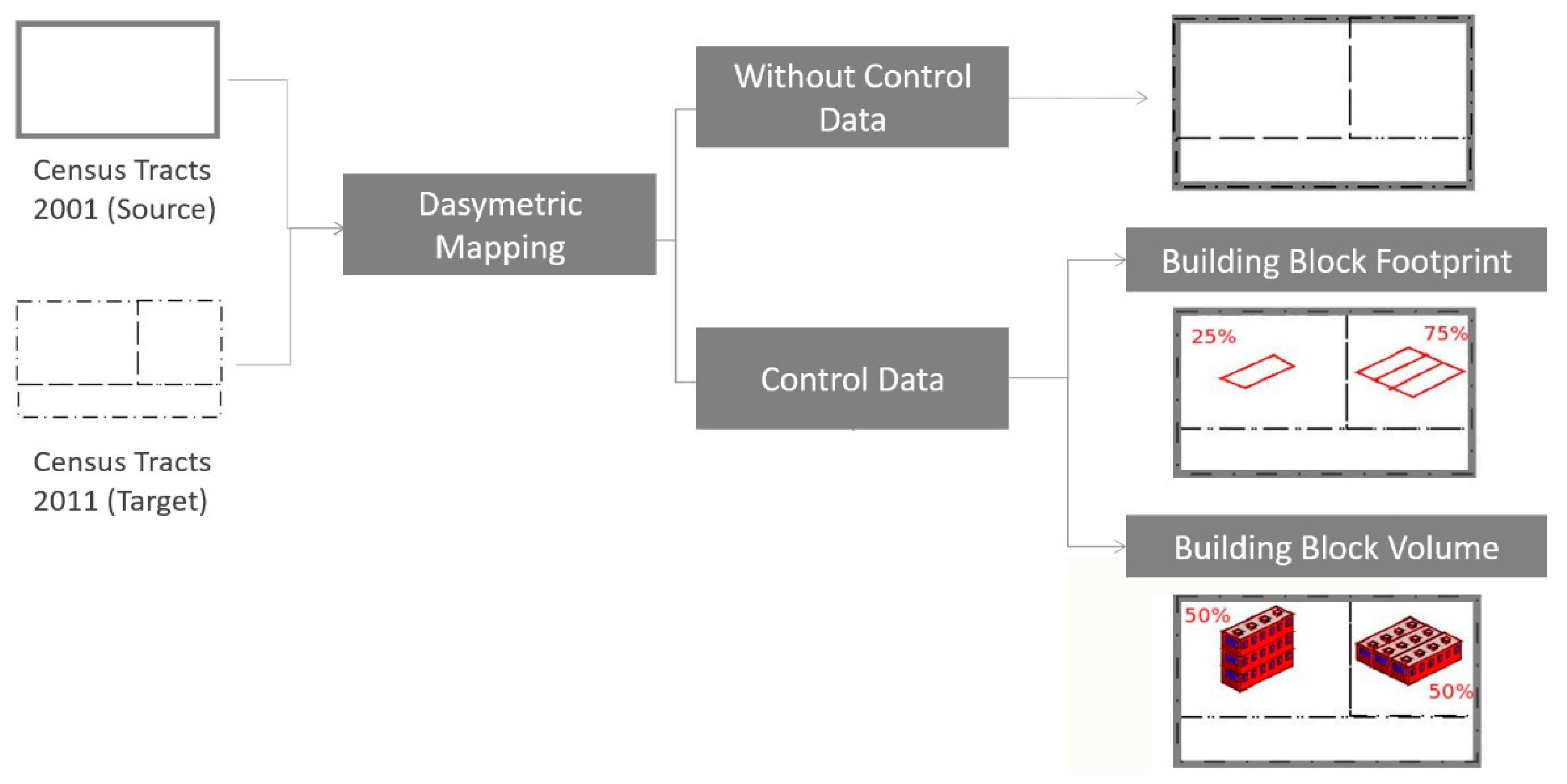
In order to evaluate the added value of working with volumetric data, three dasymetric mapping exercises were performed using different methodologies (Figure 4). The first assumed stationarity, with a homogeneous distribution of the variable of interest within each zone (census tracts); population data was re-allocated (without control data) according to the area (size) of each small area resulting from the intersection of source and target schemes. The second exercise used as ancillary data (or control data) the building block footprints extracted from the UAV point cloud, which define the area of a building block. In the final exercise, 3D information—building block volume—was used as control data, which attempts to approximate reality as the level of abstraction is reduced. As an example, consider one 2001 census tract (source dataset), which is divided into two in 2011 (Target dataset). Following the flowchart presented in Figure 4, if the 2D footprint is considered as ancillary data to compute re-allocation weights, then = 0.25 and = 0.75. However the correct weights would be 0.5 for both since the volume of both blocks is the same.
The following two subsections will discuss the methodology used to extract the 3D dataset used as control data in the dasymetric exercise, and a Monte Carlo simulation used to further explore how sensitive population estimates from the dasymetric exercise are to changes in volumetric information.
2.2.1. Control Data
The (semi)-automatic methodology developed to obtain the control data (Figure 5)—building block area and volume [13,23]—was divided into three distinct steps: (i) Point cloud data was filtered using a clustering method in order to select the set of elevation points that represent the building blocks in order to estimate the area of each block; (ii) the elevation points of terrain and eave of the building blocks were selected in order to obtain the estimated height of each building block; (iii) building block volumes were calculated using both estimated area and height.
This (semi)-automatic methodology—3DEBP—was implemented by using FOSS tools [23]. It included a set of hierarchical scripts for each step described below (Figure 5), which were proposed in R language, GRASS GIS and PostgreSQL/PostGIS, respectively.
The filtering of the UAV point cloud was performed using the clustering large applications (CLARA) algorithm [28]. CLARA is a partitioning method based on the partition of data into several sub-groups (k clusters) around k representative values (k-medoids) that are centrally located. This clustering is suitable for large datasets as is the case of 3D point clouds. The point cloud data was divided into three areas according to urban design, topography and building block types. Clustering was performed for each of these areas by using the elevation variable (z). The 3D points contained in each area were clustered into k sub-groups, which allowed us to isolate each block. The evaluation of clustering results was based on a silhouette plot analysis [29]. The implementation of the CLARA algorithm within the CLUSTER library [30] was used to obtain the clusters and silhouette plots. The latter allowed the evaluation of the clustering quality based on intra-group homogeneity and average dissimilarity. At the end of this process, the k-clusters that better represented each building block were selected (Figure 5): One cluster for area A; two clusters for area B and three clusters for area C. Next, using a concave hull algorithm implemented in GRASS [31], polygon geometries were created from the previously selected clusters. These polygons representing the building block footprints (Figure 5 and Figure 6) allowed us to calculate the total block area.
In order to estimate an average building block height, a set of spatial proximity functions were applied to the building block clusters [23] in order to: (i) Select sets of UAV points (r) that best define the eave of each building block (Figure 6) inside a one meter buffer from the block’s rooftop (concave-hull polygon), according to building block roof shape. This buffer distance is enough to remove the points that did not belong to the roof. The selection of points from corresponding clusters for each area can be represented by , where i is the block i =1,2 and A is area; and (ii) select ground points (g) from the front side of the building block ground level located (Figure 6) within a two-meter buffer from the building block’s rooftop (concave-hull polygon), according to the characteristics of the building’s surroundings (Figure 6). These ground points in area A can be represented by , where i is the block i = 1,2.
For each block, the mean elevation at ground level and of the block eaves was calculated in order to take into account the existence of extreme values. The difference between both statistics for each building block allowed us to estimate the mean building block height; hence , where i is the block number. Lastly, the volume of each building block was computed using data from the two previous stages, by multiplying the estimated area and building block height.
These steps to estimate building block height and volume were performed by a set of scripts developed by the authors using PostgreSQL/PostGIS, which are part of 3DEBP.
2.2.2. Sensitivity Analysis
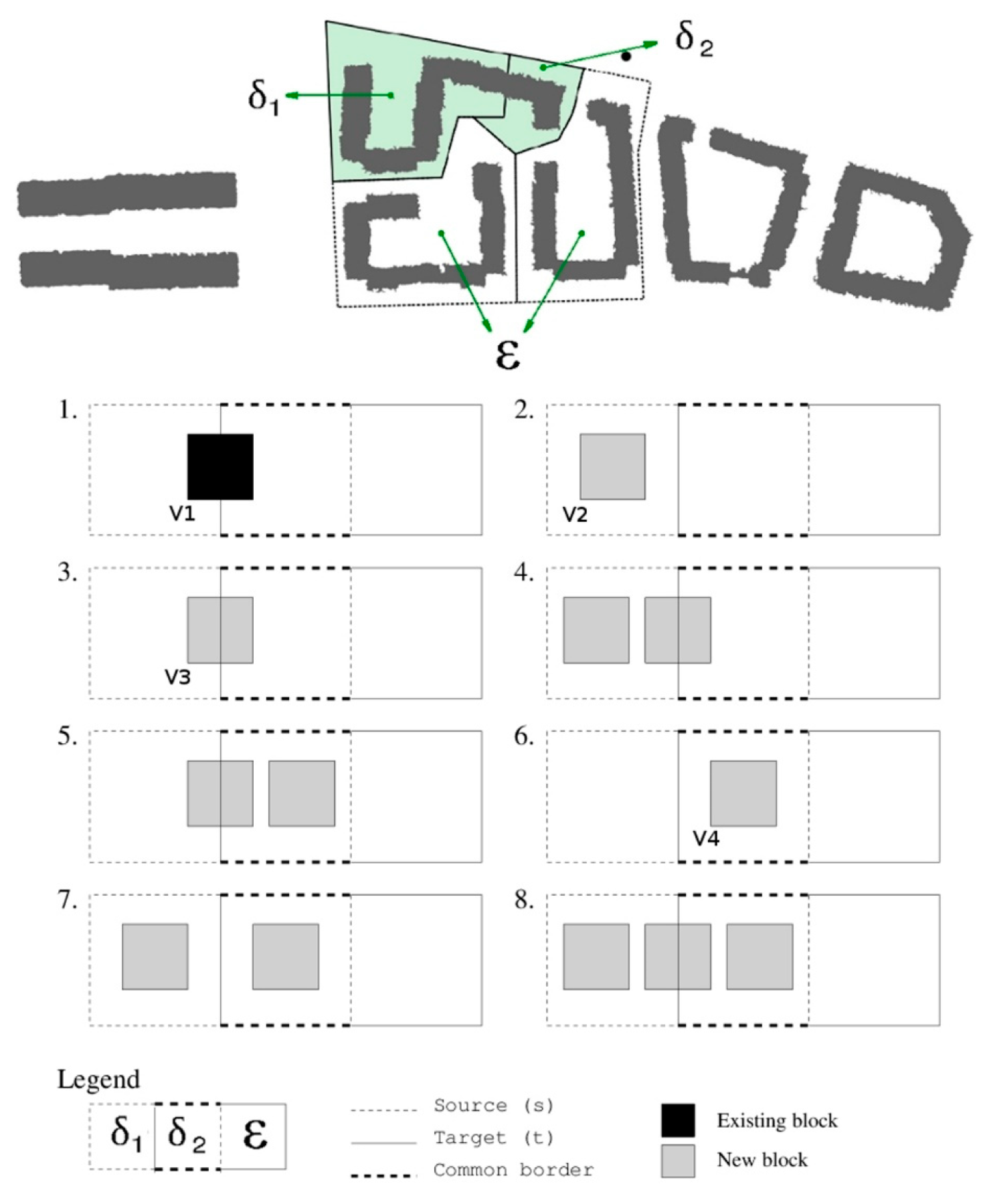
In order to test how sensitive the results from the dasymetric exercise using 3D control data are to changes in building volume or the addition of a new building block, eight distinct hypothetical scenarios were simulated.
If we assume population is a random variable then represents the estimated population for area i, while represents the expected value from averaging out all individual estimations over m runs of the algorithm (Equation (2)). Hence, we allow building volume (V) to change:
Population estimates are taken randomly as the height (hence the volume) of a chosen building is allowed to vary between the initial state, and infinity (Equation (3)). If we recall that volumetric information is the ancillary dataset that determines the result of the dasymetric exercise, increasing the volume of one building or adding a new one acts as a pulling factor, causing the population to increase in that particular area. The upper limit for population estimates is determined by the total observed population. Therefore, as the volume increases, the probability for the population to be concentrated in that particular area increases until it converges to the upper limit. The faster the rate of convergence, the more sensitive the algorithm is in respect to a particular scenario.
The dasymetric mapping exercise was performed repeatedly using a Monte Carlo simulation with building block height varying according to a set of conditions, which included simulating the effect of adding new building blocks [32]. Eight tests were performed, covering a set of distinct possible conditions/settings, as described in Figure 7.
All settings refer to situations where new buildings of varying height are added to one or two particular source zones, in this case zones SB1 and SB2 (refer back to Figure 2). This is true with the exception of condition 1, where population estimations were subject to varying height in one existing building block.
The union of SB1 and part of SB2 results in TB1 area. SB2 was itself broken into three areas—TB1, TB2 and TB3. To simplify, these zones were generalized according to the following classification scheme (Figure 7): SB1 and TB1 → ; SB2 and TB1 → ; SB2, TB2 and TB3 → . More precisely, eight tests were performed for these building blocks (Figure 7), the first test simply considered the existing building block. The conditions between test 2 and test 8 were based on the addition of new buildings to areas , or both.
The eight tests represented in Figure 7 include all possible changes between two intercepting areas, hence they provide a complete overview of possible changes in the overall results of the dasymetric exercise using volume as the ancillary variable.
The Monte Carlo analysis was performed to evaluate the effect of these conditions for the estimation of the population [32]. More precisely, maintaining the total number of residents, these were re-distributed according to an artificial increase in a particular building block or the creation of a new one, which changes the control dataset used in the dasymetric exercise.
3. Results and Discussion
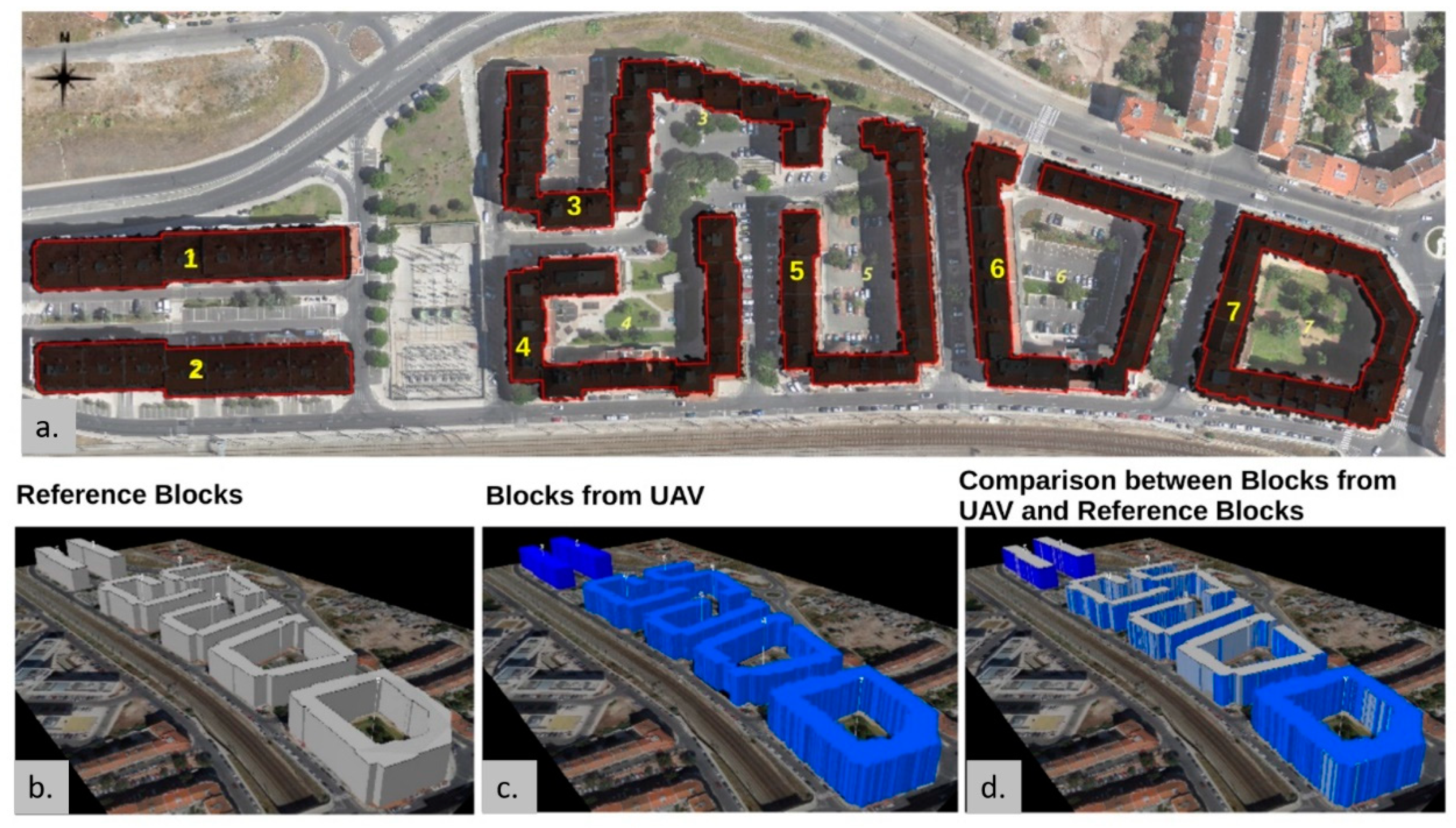
In the dasymetric mapping exercise with control data, area and volume building block parameters from the UAV point cloud were estimated. Moreover, the error associated with each parameter was calculated, using as benchmark accurate vector data acquired by photogrammetric restitution, which included building footprint or building boundary on the ground (Figure 8) and elevations (roof and terrain) for each building (Figure 6).
Table 1 shows the area and volume of each of the building blocks extracted from the UAV point cloud and the associated relative error—percentage of error represents the quality of each parameter. The building block area extracted from the UAV point cloud was overestimated for every building block, because the building blocks extracted include some elements at the rooftop, which were not included in the photogrammetric restitution—used for benchmarking, such as the top of outdoor balconies on the top floor. Building blocks in area B had the best results, with a relative error of 4.1% and 5.8%. The highest error was found in building block 7 (Figure 8), because the variations of building heights inside this block are higher.
The magnitude of absolute building block height errors (less than one meter) demonstrates that the (semi)-automatic methodology developed allows us to extract relevant and useful information from a UAV point cloud. Building block heights (except block 7) were underestimated when using the UAV dataset, with the absolute range of errors varying between 0.13 m and 0.84 m. If the maximum value of block height error were removed from the sample, it would imply a reduction to 0.36 m of average absolute height errors.
As a consequence of these results, the main source of error associated with the estimated volume is the estimated block area (Figure 8). Building block 7 had the highest relative error (about 21%), because the area error obtained for this block was high (Table 1). Building block volumes estimated in area B achieved the best results, with values ranging between 0.1% and 1.8%. The 3D visualization of block volumes (Figure 8) obtained from UAV point cloud that were generated using extruded height from the block footprint estimated have a 3D shape that is very close to the actual reference volumes, except the south facade of block 6.
Additionally, it is important to highlight that the mean error for the estimated building block volume when using accurate area value (from the reference dataset) was reduced from 5.8% to 2.8%.
After obtaining the control data from the point cloud dataset, population for 2001, distributed according to the 2011 geometrical zones, was estimated using the methodologies described—(i) areal interpolation, (ii) dasymetric mapping using 2D and (iii) dasymetric mapping using 3D control data. Table 2 shows the final results. One final column shows population estimates obtained from building point datasets. This latter dataset contains the actual number of residents per building and can therefore be used for benchmarking.
As expected, the areal interpolation results are those with the highest absolute deviation, which proves the importance of using control datasets and highlights the problems of assuming stationarity; lower performance in this case is justified since distribution within zones is assumed to be homogeneous. When the stationarity assumption is dropped, population estimates approximate the benchmark values. Note that only three zones (TB1, TB2, TB3) are affected by the changing conditions—those whose boundaries intersect existing building blocks. Moreover, the absolute deviation is lower when using 2D data than when compared with the 3D control data. Yet, given the small size of the dataset, differences are not significant. Taking into account the fact that actual building heights do not vary greatly within the study-area, large differences when adding 3D data would be probably derived from bad estimation parameters.
After comparing three methods of interpolating demographic data, a final exercise attempted to quantify the effect of overall UAV data accuracy—including omission and inclusion errors. Inclusion errors are mostly semantic (e.g., non-residential buildings to estimate population), whilst omission errors are mostly producer and processing errors (blocks filtered out during processing). As previously described, this exercise consisted in simulating a sequential increase in volume of one building and assessing the effect of estimated population using the same dasymetric methodology with 3D control data.
Figure 9 shows the results from running a number of Monte Carlo simulations according to conditions/rules one to eight (Figure 7). In these tests, population converges to a maximum value as a result of changing conditions, hence variations in the control datasets used in the dasymetric exercise. In other words, convergence represents the point when, as a result of increased building volume, the population is transported from unaffected areas to those where construction is allowed to increase.
When a new building block is inserted in SB1 (rule 2), its relative weight in terms of volume increases, but the results do not change. This is explained by the fact that no population from SB1 is re-allocated to TB1 (both constitute ). In fact, in all the tests that include changing conditions in , the results were the same as the proportional conditions (3 and 4, 5 and 8, 6 and 7). When a new building block was added in (rules 6 and 7), population increased rapidly until convergence. When one of the simulation blocks was added between and , convergence occurred but at a slower rate (rules 3 and 4, 5 and 8). In the case of rule 1, convergence is faster since, as can be seen in Figure 9, the existing block in sub-areas and was implemented mainly in the area on the left, contrary to the new blocks artificially added, with equal proportions between both sub-areas (Figure 7). If existing volume were the same between SB1 and SB2 ( and ), then results would not change. However, since the initial proportion in SB2 () was lower, a similar increase in both represents a more rapid rate of change in —which results in an increase in the estimates until convergence. This is an important result, which is deductively correct: An equal nominal increase in two parts (in this case, in the total building block volume), one being larger than the other, results in a higher relative increase in the smaller of the two. Consequently, the significance of this result is that when technical conditions change at the time of capturing primary data (e.g., UAV point-cloud), estimations using these datasets as control data are more prone to errors when both building densities and building heights are lower. In a consolidated built environment with large building footprints and height, differences between control datasets are diluted.
4. Conclusions
This work attempted to show that the use of 2D/3D control data, extracted from UAV data in dasymetric mapping, is relevant to estimate a population using dasymetric mapping techniques within urban areas. A high precision dasymetric mapping (using 3D information) was proposed to resolve the issue of multi-temporal analysis of census datasets, when there were changes in the boundaries of census tracts. Furthermore, this work highlights the usage of UAV data for the extraction of building block volume information under the development of a set of scripts based on a FOSS methodology.
The results achieved showed that the 3DEBP methodology developed for the (semi)-automatic extraction of control data (building block volume/area) using a UAV point cloud was very effective. The use of the UAV point cloud for the automatic extraction of building block units also proved very acceptable—with errors below one story—and for a clean yet not exact rendering of the built-up area. However, the extraction of accurate building block volumes depends on points selected along the eaves of roofs, which were used to compute height and area. The key issues for the successful extraction of these building parameters are: (i) The filtering methods used to remove the points that do not belong to the top of the building blocks; (ii) processing aerial image pairs to obtain a dense point cloud without gaps along the building blocks and (iii) the complexity level of building block typology and urban morphology.
As expected, the results for high precision dasymetric mapping with 3D control data were similar to those using 2D control data. This is due to the little differences in height between building blocks within the study area. As mentioned previously, this shows the consistency of the given methodology and the potential of the UAV data used, given the great heterogeneity “within” each block. The next evident step is to test the methodology in other urban morphologies, with larger heterogeneity “between” blocks (large differences in height).
The results of the sensitivity analysis conducted point in this direction, as they showed that changing existing conditions with the addition of one abnormally high block rapidly alters the estimated results, with estimated population being drawn to this new building. Furthermore, the sensitivity analysis allows us to conclude that the volume error has no impact on the results of dasymetric mapping (or estimation of population).
In future studies, the use of small study areas will again prove beneficial, as small localized phenomena can be easily studied, adding robustness to the methodology under different and more complex urban morphologies.
Author Contributions
Conceptualization, C.R., A.M.R. and J.A.T.; methodology, C.R., A.M.R.; software, C.R., A.M.R.; validation, C.R.; formal analysis, A.M.R.; writing—original draft preparation C.R.; writing—review and editing, A.M.R., J.A.T.; supervision, J.A.T.; funding acquisition, J.A.T.
Funding
This research was made with the support of CICS.NOVA—Interdisciplinary Centre of Social Sciences of the Universidade NOVA de Lisboa, UID/SOC/04647/2013, with the financial support of FCT/MCTES through National funds. The APC was funded by CICS.NOVA.
Acknowledgments
This work was made with the support of CICS.NOVA—Interdisciplinary Centre of Social Sciences of the Universidade NOVA de Lisboa, UID/SOC/04647/2013. The UAV dataset was kindly performed and provided by SINFIC company.
Conflicts of Interest
The authors declare no conflicts of interest.
References
- Talen, E. Measuring Urbanism: Issues in Smart Growth Research. J. Urban Des. 2003, 8, 195–215. [Google Scholar] [CrossRef]
- Eicher, C.L.; Brewer, C.A. Dasymetric Mapping and Areal Interpolation: Implementation and Evaluation. Cartogr. Geogr. Inf. Sci. 2001, 28, 125–138. [Google Scholar] [CrossRef]
- Holt, J.B.; Lo, C.P.; Hodler, T.W. Dasymetric Estimation of Population Density and Areal Interpolation of Census Data. Cartogr. Geogr. Inf. Sci. 2004, 31, 103–121. [Google Scholar] [CrossRef]
- Liu, L.; Peng, Z.; Wu, H.; Jiao, H.; Yu, Y. Exploring Urban Spatial Feature with Dasymetric Mapping Based on Mobile Phone Data and LUR-2SFCAe Method. Sustainability 2018, 10, 2432. [Google Scholar] [CrossRef]
- Goodchild, M.F.; Anselin, L.; Deichmann, U. A framework for the areal interpolation of socioeconomic data. Environ. Plan. A Econ. Space 1993, 25, 383–397. [Google Scholar] [CrossRef]
- Rodrigues, A.M.; Santos, T.; Deus, R.F.; Pimentel, D. Land-Use Dynamics at the Micro Level: Constructing and Analyzing Historical Datasets for the Portuguese Census Tracts. In Computational Science and Its Applications; Murgante, B., Gervasi, O., Misra, S., Nedjah, N., Rocha, A.M.A.C., Taniar, D., Apduhan, B.O., Eds.; Springer: Heidelberg, Germany, 2012; Volume 7334, pp. 565–577. ISBN 978-3-642-31075-1. [Google Scholar]
- Freedman, D.A. Ecological Inference and the Ecological Fallacy. In International Encyclopedia of the Social & Behavioral Sciences; Smelser, N.J., Baltes, P.B., Eds.; Elsevier: New York, NY, USA, 2001; Volume 6, pp. 4027–4030. [Google Scholar] [CrossRef]
- Fotheringham, A.S.; Wong, D.W.S. The Modifiable Areal Unit Problem in Multivariate Statistical Analysis. Environ. Plan. A Econ. Space 1991, 23, 1025–1044. [Google Scholar] [CrossRef]
- Hecht, R.; Herold, H.; Behnisch, M.; Jehling, M. Mapping Long-Term Dynamics of Population and Dwellings Based on a Multi-Temporal Analysis of Urban Morphologies. ISPRS Int. J. Geo-Inf. 2018, 8, 2. [Google Scholar] [CrossRef]
- Weiss, M.; Baret, F. Using 3D Point Clouds Derived from UAV RGB Imagery to Describe Vineyard 3D Macro-Structure. Remote Sens. 2017, 9, 111. [Google Scholar] [CrossRef]
- Crommelinck, S.; Bennett, R.; Gerke, M.; Nex, F.; Yang, M.Y.; Vosselman, G. Review of Automatic Feature Extraction from High-Resolution Optical Sensor Data for UAV-Based Cadastral Mapping. Remote Sens. 2016, 8, 689. [Google Scholar] [CrossRef]
- Toro, F.G.; Tsourdos, A. UAV or Drones for Remote Sensing Applications. Sensors 2018, 2. [Google Scholar] [CrossRef]
- Tenedório, J.A.; Rebelo, C.; Estanqueiro, R.; Henriques, C.D.; Marques, L.; Goncalves, J.A. New Developments in Geographical Information Technology for Urban and Spatial Planning. In Technologies for Urban and Spatial Planning: Virtual Cities and Territories; Pinto, N., Tenedório, J., Antunes, A., Cladera, J., Eds.; IGI Global: Hershey, PA, USA, 2013; pp. 196–227. [Google Scholar] [CrossRef]
- Rebelo, C.; Rodrigues, A.M.; Tenedório, J.A.; Goncalves, J.; Marnoto, J.J. Building 3D City Models: Testing and Comparing Laser Scanning and Low-Cost UAV Data Using FOSS Technologies. In Computational Science and Its Applications—ICCSA 2015; Gervasi, B., Murgante, O., Misra, B., Gavrilova, S., Rocha, M., Torre, A., Taniar, C., Apduhan, D., Eds.; Springer: Banff, AB, Canada, 2015; pp. 367–379. [Google Scholar] [CrossRef]
- Lemmens, M. Geo-Information, Technologies, Applications and the Environment; Springer: Heidelberg, Germany; Dordrecht, The Netherland; London, UK; New York, NY, USA, 2011. [Google Scholar] [CrossRef]
- Kung, O.; Strecha, C.; Beyeler, A.; Zufferey, J.C.; Floreano, D.; Fua, P.; Gervaix, F. The accuracy of Automatic Photogrammetric Techniques on Ultra-Light UAV Imagery. Int. Arch. Photogramm. Remote Sens. Spat. Inf. Sci. 2011, XXXVIII-1/C22, 125–130. [Google Scholar] [CrossRef]
- Benassi, F.; Dall’Asta, E.; Diotri, F.; Forlani, G.; Cella, U.M.; Roncella, R.; Santise, M. Testing Accuracy and Repeatability of UAV Blocks Oriented with GNSS-Supported Aerial Triangulation. Remote Sens. 2017, 9, 172. [Google Scholar] [CrossRef]
- Choi, K.; Lee, I. A Sequential Aerial Triangulation Algorithm for Real- time Georeferencing of Image Sequences Acquired by an Airborne. Remote Sens. 2013, 5, 57–82. [Google Scholar] [CrossRef]
- Haala, N.; Rothermel, M. Dense Multiple Stereo Matching of Highly Overlapping UAV Imagery. Int. Arch. Photogramm. Remote Sens. Spat. Inf. Sci. 2012, XXXIX-B1, 387–392. [Google Scholar] [CrossRef]
- Verykokou, S.; Ioannidis, C. A Photogrammetry-Based Structure from Motion Algorithm Using robust iterative bundle adjustment techniques. ISPRS Ann. Photogramm. Remote Sens. Spat. Inf. Sci. 2018, IV-4/W6, 73–80. [Google Scholar] [CrossRef]
- Wang, S.; Tian, Y.; Zhou, Y.; Liu, W.; Lin, C. Fine-Scale Population Estimation by 3D Reconstruction of Urban Residential Buildings. Sensors 2016, 16, 1755. [Google Scholar] [CrossRef] [PubMed]
- Qiu, F.; Sridharan, H.; Chun, Y. Spatial Autoregressive Models for Population Estimation at the Block Level Using LIDAR Derived Volume Information. Cartogr. Geogr. Inf. Sci. 2010, 37, 239–257. [Google Scholar] [CrossRef]
- Rebelo, C. 3D Point Clouds in Urban Planning: Developing and Releasing high-end Methodologies based on LiDAR and UAV data for the Extraction of Building Parameters. Ph.D. Thesis, Faculdade de Ciências Sociais da Universidade, Nova de Lisboa, Lisboa, July 2016. [Google Scholar]
- FOSS. Available online: http://freeopensourcesoftware.org/ (accessed on 12 January 2019).
- Censos. Available online: http://mapas.ine.pt/download/index2011.phtml (accessed on 7 March 2019).
- G8 Open Data Charter National Action Plan. Available online: https://www.gov.uk/government/publications/g8-open-data-charter-national-action-plan (accessed on 25 June 2019).
- James, M.R.; Robson, S.; d’Oleire-Oltmanns, S.; Niethammer, U. Optimising UAV topographic surveys processed with structure-from-motion: Ground control quality, quantity and bundle adjustment. Geomorphology 2017, 280, 51–66. [Google Scholar] [CrossRef] [Green Version]
- Kaufman, L.; Rousseeuw, P.J. Clustering large data sets (with discussion). In Pattern Recognition in Practice II; Gelsema, E.S., Kanal, L.N., Eds.; Elsevier: North-Holland, Amsterdam, 1986; pp. 425–437. [Google Scholar]
- Rousseeuw, P.J. Silhouettes: A Graphical aid to the interpretation and validation of cluster analysis. J. Comput. Appl. Math. 1987, 20, 53–65. [Google Scholar] [CrossRef]
- Package Cluster. Available online: https://cran.r-project.org/web/packages/cluster/cluster.pdf (accessed on 27 June 2019).
- GRASS Development Team: Geographic Resources Analysis Support System (GRASS 7) Programmer’s Manual. Open Source Geospatial Foundation. 2012. Available online: http://grass.osgeo.org/programming7/ (accessed on 7 July 2019).
- Fisher, P.F.; Langford, M. Modelling the Errors in Areal Interpolation between Zonal Systems by Monte Carlo Simulation. Environ. Plan. A Econ. Space 1995, 27, 211–224. [Google Scholar] [CrossRef]
Figure 1.
Study area with census tracts and building footprints.
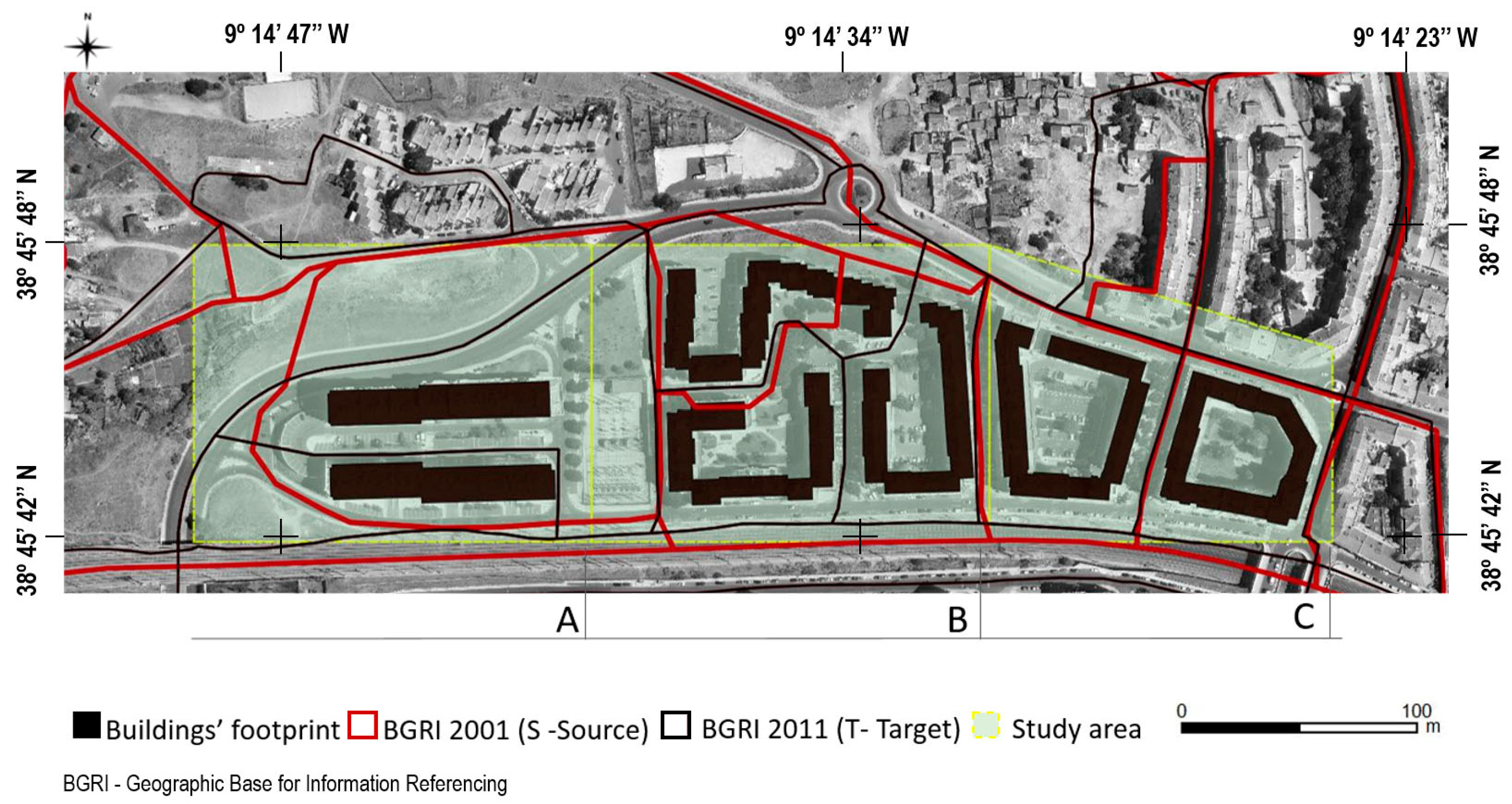
Figure 2.
Census tracts: Source (Geographic Base for Information Referencing—BGRI 2001) and target (BGRI 2011).
Figure 2.
Census tracts: Source (Geographic Base for Information Referencing—BGRI 2001) and target (BGRI 2011).
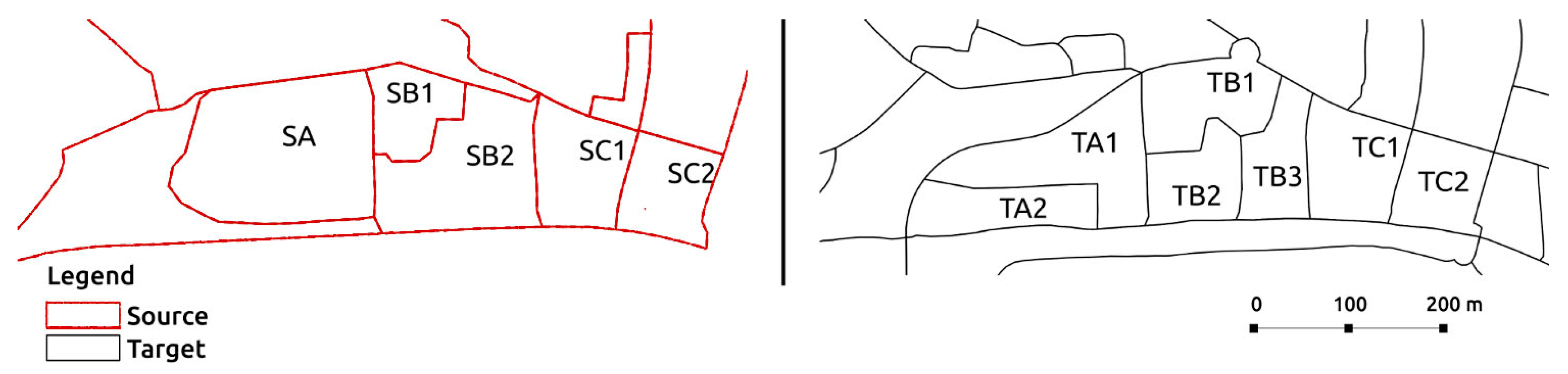
Figure 3.
Trajectory flight lines performed by Swinglet CAM.
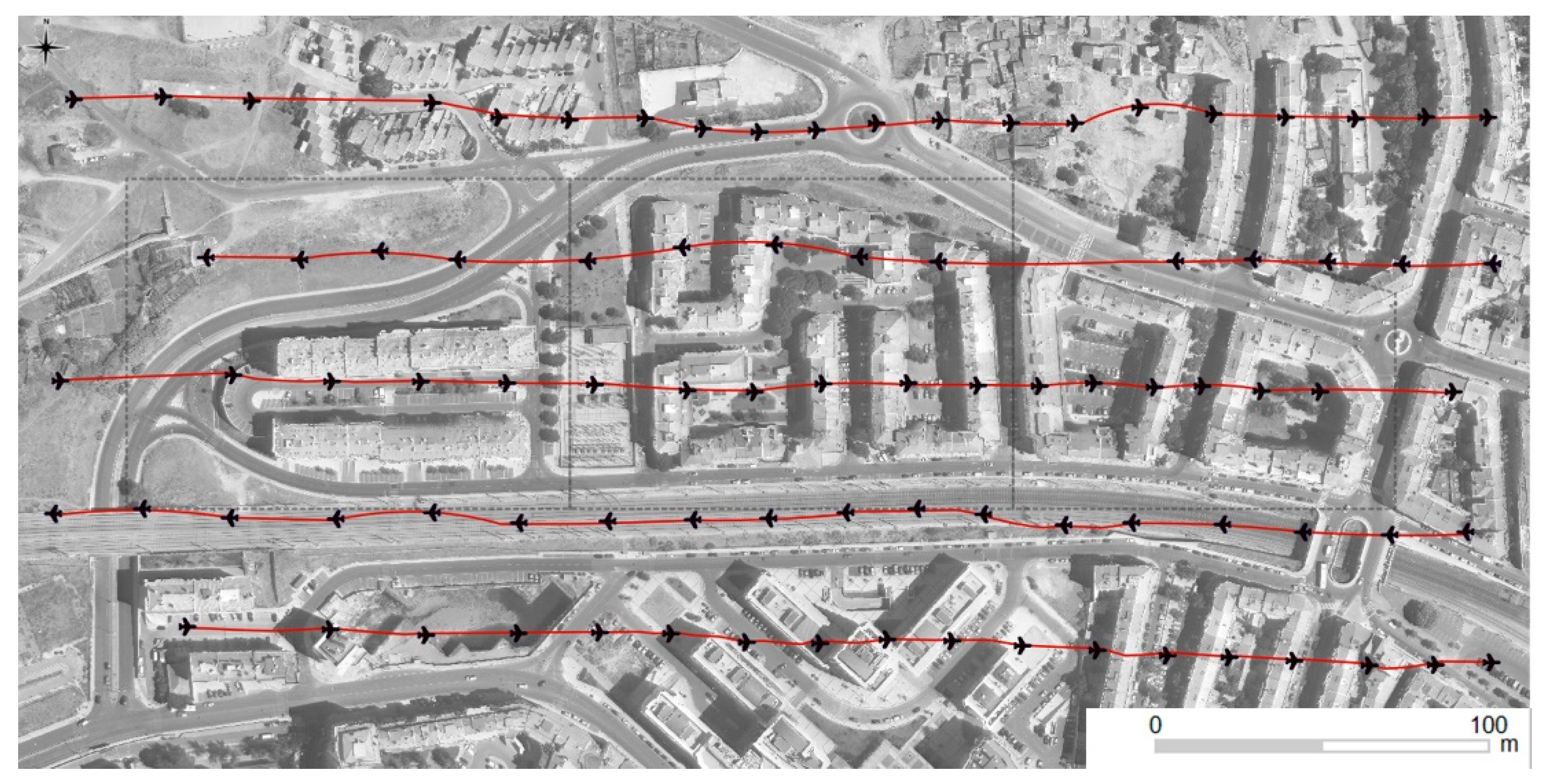
Figure 4.
Summary flowchart.

Figure 5.
Methodological approach to building block volume extraction—3DEBP—based on a 3D Point Cloud.
Figure 5.
Methodological approach to building block volume extraction—3DEBP—based on a 3D Point Cloud.
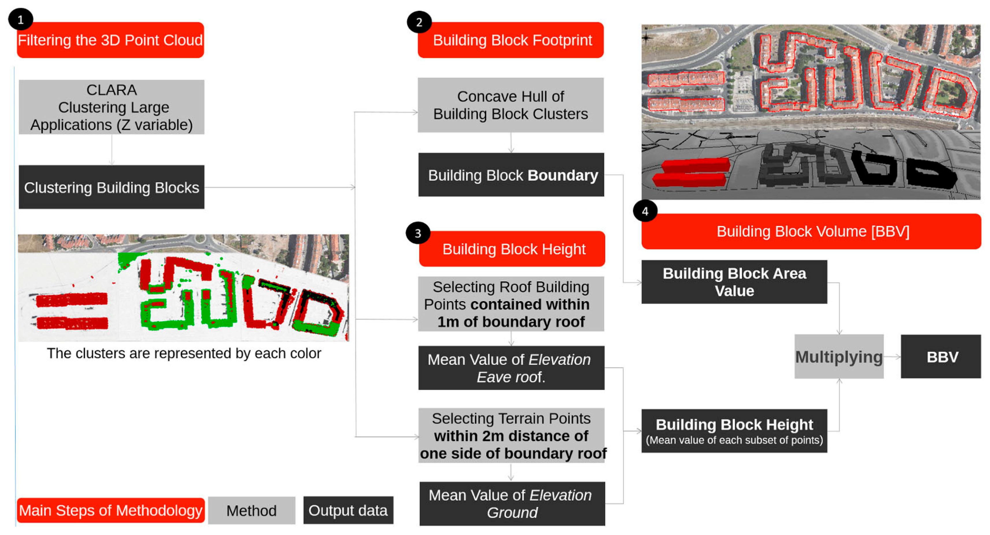
Figure 6.
Points selected (eave roof and ground) for each block in area A.
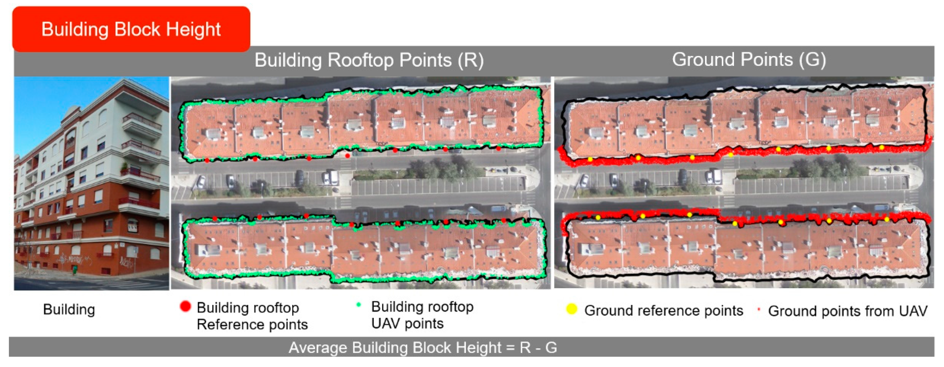
Figure 7.
Sensitivity analysis performed using blocks (V1, V2, V3 and V4) changing block height.

Figure 8.
2D/3D comparison between reference data and data estimated from UAV: (a) Building block footprints (red: Reference dataset; black: extracted from UAV dataset); (b) 3D block model obtained from reference dataset; (c) 3D block model obtained from UAV data and (d) combination of the two 3D models represented in b, c).

Figure 9.
Results of the Monte Carlo simulation.


Table 1.
Building block parameters (area, height and volume) estimated from unmanned aerial vehicle (UAV) and the error obtained in this estimation.
Table 1.
Building block parameters (area, height and volume) estimated from unmanned aerial vehicle (UAV) and the error obtained in this estimation.
| Area | Building Block | Area (m2) | Height (m) | Volume (m3) | Error Area (%) | Error Height (m) | Error Volume (%) |
|---|---|---|---|---|---|---|---|
| A | 1 | 2473.92 | 18.65 | 46,139 | 10.4 | −0.13 | 9.7 |
| 2 | 2410.50 | 15.35 | 37,001 | 6.3 | −0.52 | 2.8 | |
| B | 3 | 3206.12 | 14.51 | 46,521 | 6.1 | −0.73 | 1.0 |
| 4 | 2665.80 | 15.03 | 40,067 | 5.8 | −0.84 | 0.1 | |
| 5 | 2614.84 | 13.78 | 36,033 | 4.1 | −0.31 | 1.8 | |
| C | 6 | 3175.61 | 14.28 | 45,348 | 6.6 | −0.31 | 4.4 |
| 7 | 3175.02 | 15.75 | 50,007 | 19.3 | +0.16 | 20.5 |
Table 2.
Estimated population in 2001 according to 2011 census tracts (refer to Figure 2).
Table 2.
Estimated population in 2001 according to 2011 census tracts (refer to Figure 2).
| Control Data | ||||
|---|---|---|---|---|
| Zones | Area Interpolation | 2D | 3D | Benchmark 1 |
| TA1 | 4 | 0 | 0 | 0 |
| TA2 | 14 | 0 | 0 | 0 |
| TB1 | 374 | 379 | 380 | 367 |
| TB2 | 327 | 342 | 356 | 348 |
| TB3 | 312 | 336 | 321 | 343 |
| TC1 | 486 | 498 | 498 | 498 |
| TC2 | 350 | 384 | 384 | 384 |
| Absolute Deviation | 17.53 | 3.66 | 6.32 | 0 |
1 Estimated from dwellings.
© 2019 by the authors. Licensee MDPI, Basel, Switzerland. This article is an open access article distributed under the terms and conditions of the Creative Commons Attribution (CC BY) license (http://creativecommons.org/licenses/by/4.0/).
Share and Cite
MDPI and ACS Style
Rebelo, C.; Rodrigues, A.M.; Tenedório, J.A. Dasymetric Mapping Using UAV High Resolution 3D Data within Urban Areas. Remote Sens. 2019, 11, 1716. https://0-doi-org.brum.beds.ac.uk/10.3390/rs11141716
AMA Style
Rebelo C, Rodrigues AM, Tenedório JA. Dasymetric Mapping Using UAV High Resolution 3D Data within Urban Areas. Remote Sensing. 2019; 11(14):1716. https://0-doi-org.brum.beds.ac.uk/10.3390/rs11141716
Chicago/Turabian StyleRebelo, Carla, António Manuel Rodrigues, and José António Tenedório. 2019. "Dasymetric Mapping Using UAV High Resolution 3D Data within Urban Areas" Remote Sensing 11, no. 14: 1716. https://0-doi-org.brum.beds.ac.uk/10.3390/rs11141716
Note that from the first issue of 2016, this journal uses article numbers instead of page numbers. See further details here.