Evaluating the Variability of Urban Land Surface Temperatures Using Drone Observations


Department of Civil, Construction & Environmental Engineering, Marquette University, P.O. Box 1881, Milwaukee, WI 53211, USA
*
Author to whom correspondence should be addressed.
Remote Sens. 2019, 11(14), 1722; https://0-doi-org.brum.beds.ac.uk/10.3390/rs11141722
Submission received: 30 May 2019
/
Revised: 12 July 2019
/
Accepted: 16 July 2019
/
Published: 20 July 2019
(This article belongs to the Special Issue Remote Sensing Monitoring of Land Surface Temperature (LST))
Abstract
:Urbanization and climate change are driving increases in urban land surface temperatures that pose a threat to human and environmental health. To address this challenge, we must be able to observe land surface temperatures within spatially complex urban environments. However, many existing remote sensing studies are based upon satellite or aerial imagery that capture temperature at coarse resolutions that fail to capture the spatial complexities of urban land surfaces that can change at a sub-meter resolution. This study seeks to fill this gap by evaluating the spatial variability of land surface temperatures through drone thermal imagery captured at high-resolutions (13 cm). In this study, flights were conducted using a quadcopter drone and thermal camera at two case study locations in Milwaukee, Wisconsin and El Paso, Texas. Results indicate that land use types exhibit significant variability in their surface temperatures (3.9–15.8 °C) and that this variability is influenced by surface material properties, traffic, weather and urban geometry. Air temperature and solar radiation were statistically significant predictors of land surface temperature (R2 0.37–0.84) but the predictive power of the models was lower for land use types that were heavily impacted by pedestrian or vehicular traffic. The findings from this study ultimately elucidate factors that contribute to land surface temperature variability in the urban environment, which can be applied to develop better temperature mitigation practices to protect human and environmental health.
1. Introduction
Urban areas across the world are subject to thermal stresses caused by the surface urban heat island (SUHI) effect where urban land surfaces experience higher temperatures than their surrounding rural areas. This is in large part due to the replacement of undeveloped vegetated land with anthropogenic materials that absorb more solar radiation and have different heat capacity and surface radiative properties [1]. This results in higher surface temperatures that pose a significant threat to human health [2], as well as higher storm runoff temperatures that can harm aquatic life [3,4,5]. These stresses are only expected to grow with increases in global temperatures and urban populations; therefore, it is critical that we understand the fundamental processes that drive land surface temperature (LST) to develop solutions that can protect human and environmental health.
To that end, thermal remote sensing is an important tool for evaluating urban land surface temperatures. This includes satellite sensors such as ASTER, MODIS and Landsat that can capture land surface temperatures at 30 m–1 km resolutions [6]. Data from these satellites have been used to extensively study urban land surface temperatures and their effects [7,8,9,10,11,12,13,14]. However, while satellite remote sensing is valuable for evaluating LST across a city scale, the spatial resolution precludes its applications to smaller spatial scales that better reflect the spatial complexity of the urban environment. To acquire higher resolution thermal data, studies have used aerial reconnaissance or downscaling techniques [15,16]; however, these are still at resolutions (4–10 m) that cannot capture changes that occur on a sub meter resolution. Furthermore, satellite remote sensing is temporally constrained to intervals between 1–14 days. Aerial flights do not have the same temporal constraints; however, doing so at on-demand temporal resolutions would not be economically practical. Therefore, these methods are inadequate for evaluating changes in urban LST that occur throughout the day or capturing the spatial heterogeneity of urban LST at small scales.
This challenge is important to overcome as urban land surfaces are spatially complex and significant variations in land cover can occur on a sub meter spatial resolution [17]. While existing research has demonstrated that the spatial configuration of land use classifications at a city scale are important (i.e. industrial, residential, forest) [18,19], less is known about the importance of the spatial configuration and variations in LST at smaller scales (i.e., sidewalks, grass medians, flowerbeds, etc.). In addition, the urban environment is dynamic and land surface temperatures can be significantly influenced by other factors besides land cover material properties [20]. Land surface temperature may therefore vary significantly across small spatial scales; however, the factors that control this variation are not well defined. Doing so requires direct measurements of surface temperatures across wide spatial and temporal scales, yet little research to date has evaluated the spatial variability in temperature among urban land use types in sub-meter resolutions. This may be due to measurement limitations, as satellite data is too coarse and in-situ temperature probes are too expensive to densely distribute across an urban landscape. Therefore, new and innovative approaches to measuring land surface temperatures at small spatial and temporal scales are needed to assess thermal variability across land use types in the urban environment.
Unmanned Aerial Vehicles (UAVs) or drones, are a technology that can meet this challenge. Recent advances in UAVs and radiometric thermal cameras have made it possible to capture land surface temperatures on-demand and at sub-meter spatial resolutions that accurately reflect the spatial complexity and detail of land surface temperatures in the urban environment [21]. UAVs also have advantages in that they can be flown on demand to capture LST at temporal resolutions unmatched by satellite or aerial imagery. While the limited battery life of around 30 minutes for quad-copter UAVs constrains the area that can be captured in a single flight, their spatial and temporal resolutions offer significant advantages for evaluating the variability of LST in the urban environment at fine spatial and temporal scales.
We therefore present a study to evaluate the variability of temperatures across urban land surfaces using a UAV. In this study, we apply a UAV and radiometric thermal camera to capture land surface temperatures at high-resolutions (13 cm) in two case study locations: Milwaukee, Wisconsin and El Paso, Texas. Using data collected throughout a calendar year, we evaluate the variability in land surface temperatures, develop models to predict mean land surface temperature based upon weather parameters and evaluate the diurnal trends in urban land surface temperature. To do so, we (1) quantify land surface temperature variability across different surface types, (2) evaluate variance in temperature across different surface types based upon meteorological and/or other derived parameters (e.g., albedo, normalized difference vegetation index, apparent thermal inertia, etc.), (3) predict land surface temperature based upon meteorological parameters and (4) assess diurnal variability in land surface temperature magnitude and uncertainty. Ultimately, this study helps to elucidate factors that contribute to land surface temperature variability in the urban environment at small spatial scales, which can then be applied to develop better temperature mitigation strategies.
2. Materials and Methods
2.1. Case Study Locations
Two case study locations were chosen for this project: (1) a portion of Marquette University’s campus in Milwaukee, WI and (2) a portion University of Texas El Paso’s (UTEP) campus in El Paso, Texas (Figure 1). The Marquette and UTEP case study areas were roughly 21,300 m2 and 27,300 m2, respectively and included a balance of both natural landscape and impervious gray surfaces. Surface types within each case study location were manually delineated using ESRI’s ArcMap software. The nine surfaces types identified at Marquette and UTEP and their respective surface areas are listed in Table 1. The specific locations on each campus were chosen for their variety of surface types, similarities in land use between the two locations and suitability for drone takeoff/landing and flying. In addition, these locations provide a contrast in geography, climate and weather that are helpful in testing the generalizability of our findings. For example, Milwaukee’s climate is classified by Koppen and Geiger as Dfa (Humid Continental Hot Summers With Year Around Precipitation) and receives 870 mm of precipitation annually, while El Paso is classified as BWk (Cold Desert Climate) and receives 221 mm of precipitation annually [22,23].
2.2. Equipment
Remote sensing data was collected using a DJI Matrice 100 (M100) quadcopter UAV. The M100 was deployed at our case study locations with three types of camera payloads—visual, multispectral and infrared. These cameras include the DJI Zenmuse X3 visual (12 MP), Zenmuse X3 multispectral (Blue-Green-NIR 680–800 nm at 12 MP) and DJI Zenmuse XTR radiometric thermal (13 mm, 30 Hz and spectral bandwidth of 7–13 µm). Additionally, ground temperatures were validated using a Nubee NUB8380 Digital Infrared Thermometer.
2.3. Data Collection Methods
Two datasets were collected during the 2018 calendar year: (1) surface temperature measured at 12:00 PM across the entire year and (2) surface temperature measured on a diurnal cycle. To evaluate surface temperature across the entire year, fourteen flights in Milwaukee and one in El Paso were recorded between 26 February and 13 September 2018 (Table 2). To evaluate the diurnal cycle of temperature, three flights in Milwaukee and one in El Paso measured temperature throughout the day at 9:00 AM, 12:00 PM, 3:00 PM and 5:00 PM (Table 3). Weather data was collected at Marquette from a station on top of Engineering Hall and weather data at UTEP was collected from a weather station 10.5 km away at El Paso International Airport. Each station recorded air temperature, relative humidity, wind speed, wind direction, relative humidity, solar radiation and atmospheric pressure. Drone imagery was captured autonomously using a third-party photogrammetry software called Pix4Dcapture. Using this software, autonomous flight paths were programmed to the drone prior to each mission. Programmed flight path information included drone speed, altitude and image overlap. Drone speed was set at 54 km/h for visual and multispectral flights but set at a lower threshold of 30.6 km/h for thermal flights due to the difference in image capture speed between the two camera technologies. The flight altitude for each mission was set to the United States Federal Aviation Administration (FAA) maximum allowable limit of 120 m, which resulted in thermal imagery at a 13 cm pixel size. Finally, the image overlap was set to 85%, which provided reliable overlap for stitching an orthomosaic during data processing.
2.4. Thermal Data Processing
After data collection in the field, a series of post-processing steps were performed using Pix4D and ESRI’s ArcMap to stitch the drone thermal imagery into orthomosaics, correct temperature values for emissivity and extract surface temperature data for analysis. First, Pix4D was used to stitch the captured thermal images into orthomosaics, export the orthomosaics as a 32-bit TIFF and georeference them for application within ArcMap.
Once in ArcMap, an emissivity correction was applied to each thermal orthomosaic. Emissivity is a measure of how well a material can emit energy as thermal radiation and different materials have different values of emissivity depending on their surface properties [24]. Land use classifications that were previously delineated for each case study area were used to apply emissivity values to the target surfaces. The emissivity values for each land use classification used in this study are listed in Table 4 and are based upon a review of emissivity studies. These emissivity values were then applied in the following emissivity correction equation derived from Stefan-Boltzmann Law:
where Ttarget is the actual temperature of the target surface [K], Tsensor is the temperature measured by the infrared camera [K], Tbackground is the recorded air temperature [K] and ε is the emissivity value of the target surface [25]. This equation was used to correct each surface type for their respective emissivity before performing spatial data analysis.
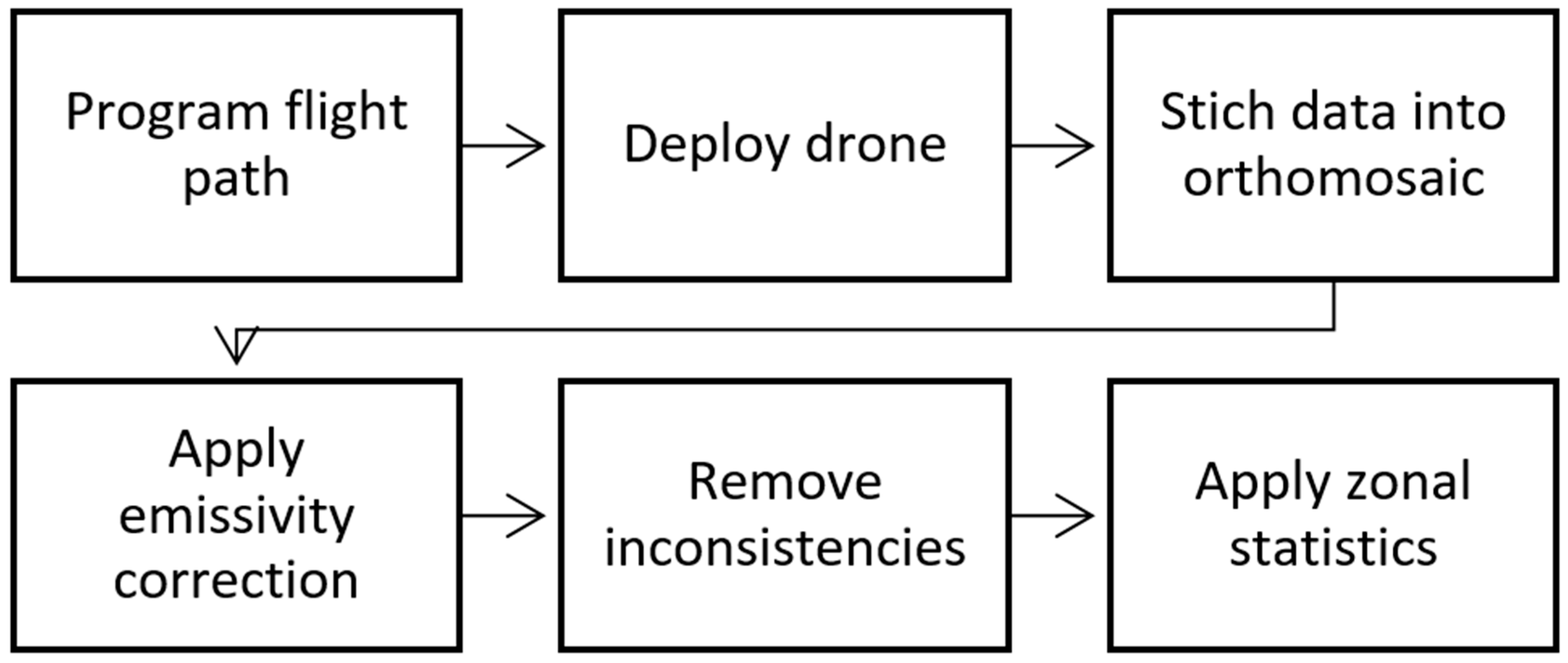
Once the thermal data were corrected for emissivity, spatial data analysis was performed in ArcMap. First, a land use feature map was created that categorized the surface types in each case study location. Then inconsistencies within these areas, such as a parked car within a parking lot, human traffic on a sidewalk or construction materials on the street, were clipped and removed for each flight. Once these inconsistencies were removed, zonal statistics was applied to compute summary statistics of each surface type such as mean and standard deviation of the land surface temperature. A complete flow-chart of the process from flight programming to developing summary statistics is shown in Figure 2. In total this process took about 3 h to complete for each flight.
2.5. Surface Parameters
In addition to surface temperature, three other material properties were derived from visual and multispectral imagery, converted into spatial distribution rasters and averaged for each surface type. These include albedo (S), normalized difference vegetation index (NDVI) and apparent thermal inertia (ATI). Albedo, a measure of solar reflectance of a material, was derived from blue, green, red and near-IR image bands as shown in the following equation:
where cb = 0.17, cg = −0.13, cr = 0.33 and ci = 0.54 are derived constants and bk, gk, rk and ik are the band reflectance’s for—blue, bk (420–492 nm); green, gk (533–587 nm); red, rk (604–664 nm); and near-IR, ik (833–920 nm) [34].
Visual and multispectral imagery were also used to derive NDVI, which is a measure of the degree of live vegetation and is commonly used to evaluate soil moisture dynamics, erosion potential and plant and crop health. As shown in Equation (3), NDVI is a function of near-IR and red band reflectance and is estimated on a scale of −1 to +1, with higher values indicating higher vegetative cover and greater plant health [35].
Finally, ATI was derived for each surface type from albedo (S), solar correction (SCR) and the diurnal temperature amplitude (DTA) (Equation (4)). ATI is an estimation of thermal inertia from remotely sensed observations and can be estimated from diurnal changes in temperature. Specifically, ATI is derived from solar correction (SCR), albedo (S) and the diurnal temperature amplitude (DTA), where DTA is the difference between the maximum and minimum surface temperature recorded at the time the remote images were captured and SCR is the solar correction factor (Equation (5)), which is dependent on geographic location, the local latitude (θ) and the solar declination (φ) [36].
2.6. Model Development
Drone observations were applied to develop empirical models of land surface temperature. These include (1) a regression model to predict spatially averaged surface temperatures at 12:00 PM based upon meteorological variables and (2) a model to assess diurnal variability and predict surface temperatures throughout a given day.
Multi-variable regression models were developed to predict spatially averaged surface temperature of the fourteen Milwaukee and single El Paso 12:00 PM flights using MATLAB and the statistical software package JMP 13 [37]. Response screening was performed for each of the respective datasets to identify the strength of relationship between surface temperature (response) and meteorological parameters (predictors). Between the two case study locations, six surface types that were common to both locations were used as response variables: grass, canopy cover, concrete parking lot, concrete sidewalk, composite rooftop and road surface. Meteorological predictor variables included air temperature, relative humidity, preceding 24 h rainfall, wind speed, wind direction, barometric pressure and solar radiation. After response screening, stepwise linear regression was then performed to predict land surface temperature based upon meteorological parameters as represented in following equation:
where y is the response variable, β0, β1, …, βk are the regression coefficients and x1, x2, …, xk are the predictor variables for k predictors [38]. These models were developed using data from both the Milwaukee and El Paso flights; therefore, to evaluate the influence and leverage of the El Paso dataset we computed Cook’s D influence and hat matrix leverage statistics [38].
Finally, we explored the variation in surface temperatures as they change throughout the day (9 AM, 12 PM, 3 PM and 5 PM) and evaluated if this variation could be explained by any meteorological parameters. In addition to exploring diurnal changes in variability, we applied the data to develop a model to predict land surface temperatures throughout the day for the six land use types common to each location. To do so, we applied the drone data collected on the four diurnal flight missions to estimate land surface temperatures based upon the solar radiation and the difference between the air and land surface temperatures, which have been found to be statistically significant predictors for diurnal estimates of pavement temperatures [39].
First, we computed a parameter (g) based upon the drone-derived mean land surface temperature and measured air temperature and solar radiation:
where is the mean surface temperature of the land use, Ta is the measured air temperature and S is the measured solar radiation (kW). Next, g at a given hour i was estimated using a Gaussian peak model given by the following:
where gi, is the parameter g at hour i, a is the peak value, b is the critical point and c is the growth rate [40]. Using this model, the mean land surface temperature can be predicted based upon air temperature and solar radiation for any time of day using the following:
where Ts,i is the estimated surface temperature at hour i and Ta,i and Si are the air temperature and solar radiation at hour i. Taken as a whole, these models test both the suitability of predicting drone-derived mean land surface temperatures based upon meteorological variables, as well as the generalizability of our findings by including data from sites in two different geomorphologic and climatic regions.
3. Results
3.1. Surface Temperature Variability
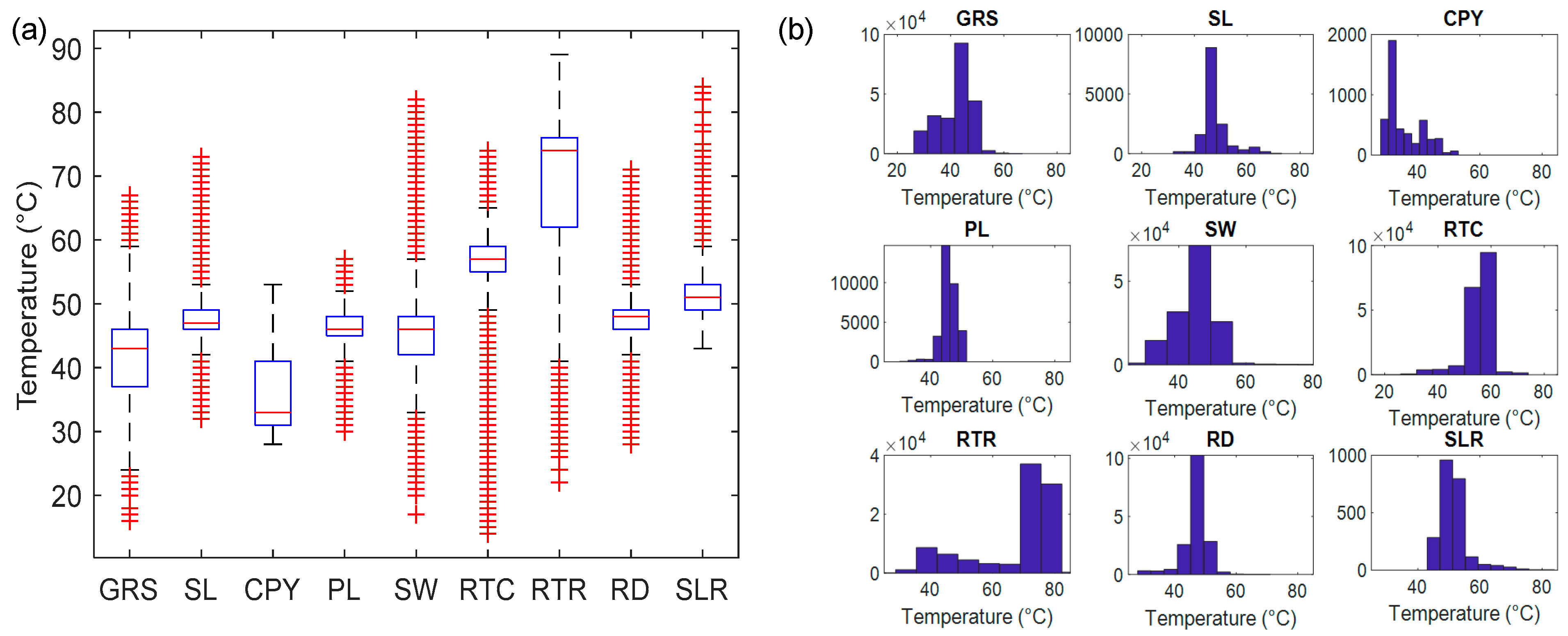
We evaluated the land surface temperature variability of each flight across common land use types and generally found that green surfaces had a greater degree of variability than gray surfaces, with the exception being the rubber rooftop. As an example, the distribution of surface temperature data (1,986,543 total data points) is shown in Figure 3 for a flight recorded on July 11, 2018. The six gray surfaces recorded a smaller distribution of temperature on average but had more extreme values than green surfaces (Figure 3a). Gray surfaces retain more heat from the sun because of their high emissivity and ATI and therefore typically have higher surface temperatures. Additionally, non-normal behavior was identified for both canopy cover and rubber rooftop (Figure 3b). Canopy cover exhibits a left skew while the rubber rooftop exhibits a right skew. The canopy cover had a variation of tree types and therefore a variation of leaf area indices (LAI), which may be a reason for the skew in the temperature data. The rubber rooftop also exhibited a strong right skew, which may be due to small materials on the roof surface, such as ventilation pipes and drainage grates, that were difficult to detect and may not have been removed from the dataset. Therefore, this caused a distribution of lower temperatures to be recorded.
We then summarized the average temperature, standard deviation and coefficient of variation of each surface type for the fourteen recorded flights in Milwaukee, WI and the single flight in El Paso, TX (Table 5). Generally, gray surfaces exhibited higher temperatures throughout the year than green surfaces. In El Paso, the asphalt parking lot exhibited the highest average temperature (51.7 °C) and grass exhibited the lowest (41.6 °C), while in Milwaukee the black rubber rooftop exhibited the highest average temperature (57.4 °C) and canopy cover exhibited the lowest (30.4 °C). In terms of variation, the lowest degrees of variation typically occurred in the parking lots and grass. However, there is a noted difference in the variation between the two locations; the road in Milwaukee had the highest coefficient of variation of 0.32, while the road in El Paso had the lowest at 0.04. This may be due to a difference in traffic on the days that flights were conducted. The location in Milwaukee is located near the city center and is subject to heavy and constant vehicular traffic, while the location in El Paso is in a restricted traffic area and experienced very low vehicle activity on the weekend that the flight was conducted.
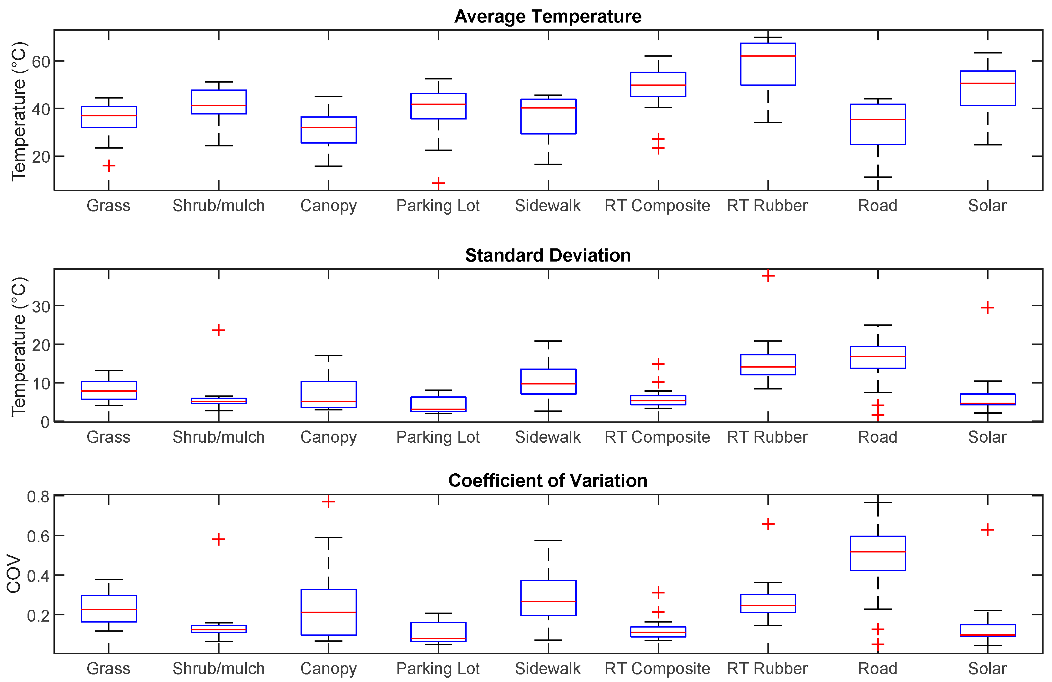
The distribution of the average temperature, standard deviation and coefficient of variation for the fourteen Milwaukee, WI flights is further illustrated in Figure 4. The shrub/mulch, composite rooftop and solar panels have the most consistent variability among the land use types as shown in the boxplot distribution of their coefficient of variation, while the greatest spread in variation occurred in the road and sidewalk. This may indicate that areas that are not subject to human traffic (e.g., shrub/mulch flower beds, rooftops and solar panels) have more consistent variability in their temperatures, while other areas that are subject to intermittent human traffic (e.g., roads and sidewalks) have inconsistent temperature variabilities. We also evaluated if the variability in land surface temperature correlated with any meteorological parameters but found no statistically significant predictors.
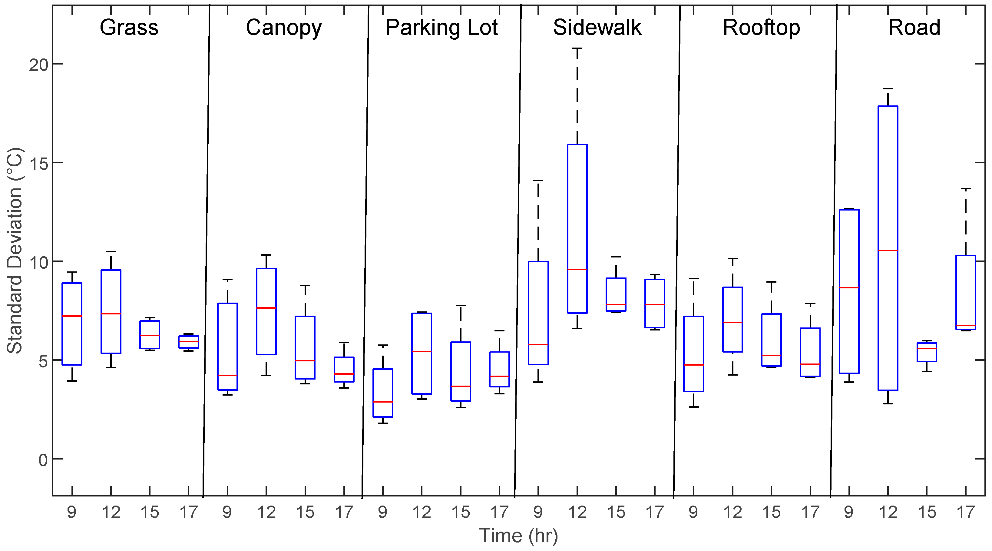
We evaluated the variation in surface temperatures throughout the day and found that the highest degree of variation occurred at noon. This is demonstrated in the Figure 5, which shows box plots of the standard deviation for six land use types: grass, canopy, parking lot, sidewalk, composite roof and road for data from both MU and UTEP. As illustrated, all land use types have the greatest standard deviation in temperatures during 12:00 PM, with lower levels of deviation in the morning and late afternoon. This trend suggests that as surfaces heat up, they do so at different rates, which contributes to more variability during mid-day.
3.2. Impact of the Built Environment
We also evaluated the spatial distribution of surface temperature to locate and identify factors of the built environment that contribute to temperature variability. Figure 5 illustrates the spatial distribution of surface temperatures for a flight on July 8th, 2018. One factor of variability is the reflectance and shaded cover from nearby buildings. For example, sidewalks in close proximity to Engineering Hall exhibited higher temperatures, most likely due to the sun’s reflectance off its glass paneling. Two similarly sized sidewalk areas were compared and results show the average temperature was 4.7 °C hotter for the location closer to the building than the one farther away. In comparison to the sidewalk, parking lot land uses had more consistent variability, perhaps because there were fewer nearby buildings or large trees to exacerbate (glass reflectance) or reduce (shaded cover) their temperature. This indicates proximity to nearby buildings or other structures can be a significant factor of uncertainty in predicting surface temperatures.
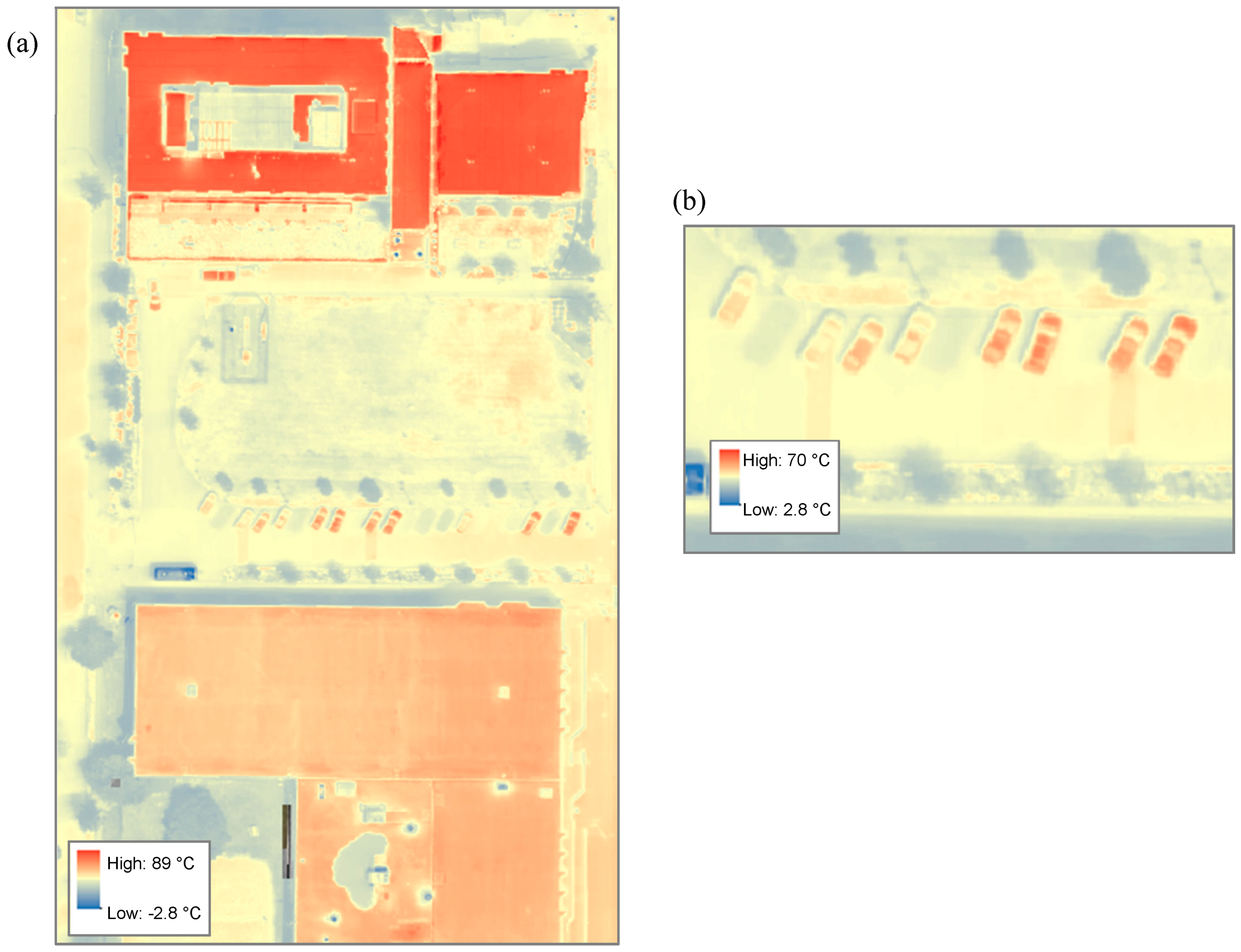
Other sources of land surface temperature uncertainty are traffic and parked cars. Traffic flow along a roadway intermittently blocks the suns radiation, thereby impacting the surface temperatures of the roadway pavement below. This creates a concentrated pocket of cooler surface temperatures called a heat shadow, which results in variations in surface temperatures across the pavement. This is especially pronounced in pavement lots with parked cars as illustrated in Figure 6b, which shows the distribution of surface temperatures within a parking lot. In this figure a parked car rooftop, pavement surface and heat shadow recorded temperatures of 69.6 °C, 47.8 °C and 49.0 °C, respectively, all within a space of ~50 m2.
3.3. Surface Properties and Land Surface Temperature
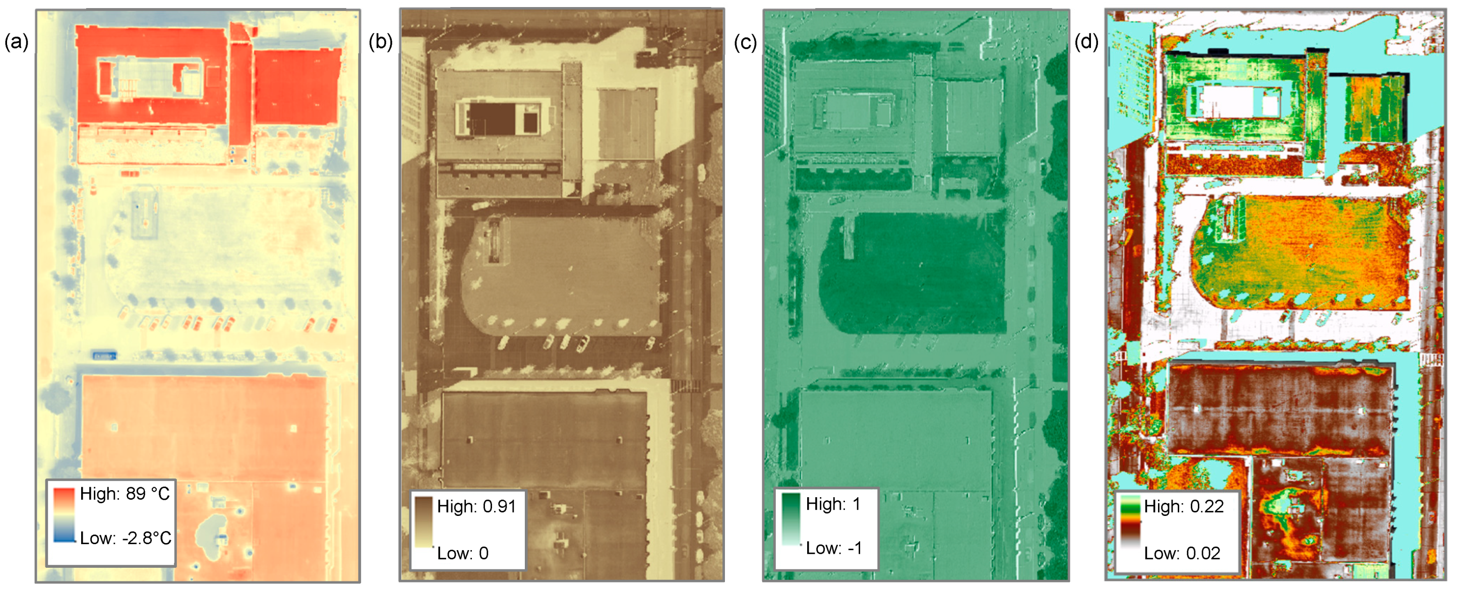
Drone data was applied to derive surface properties including albedo, NDVI and ATI, of the surface types in the case study (Table 6). The light concrete parking lot exhibited the highest albedo (0.673) while grass exhibited the lowest (0.317). The spatial distribution of temperature, albedo, NDVI and ATI at the Milwaukee, WI case study location is shown in Figure 7. As illustrated, these surface material properties have a large degree of variation across the case study area.
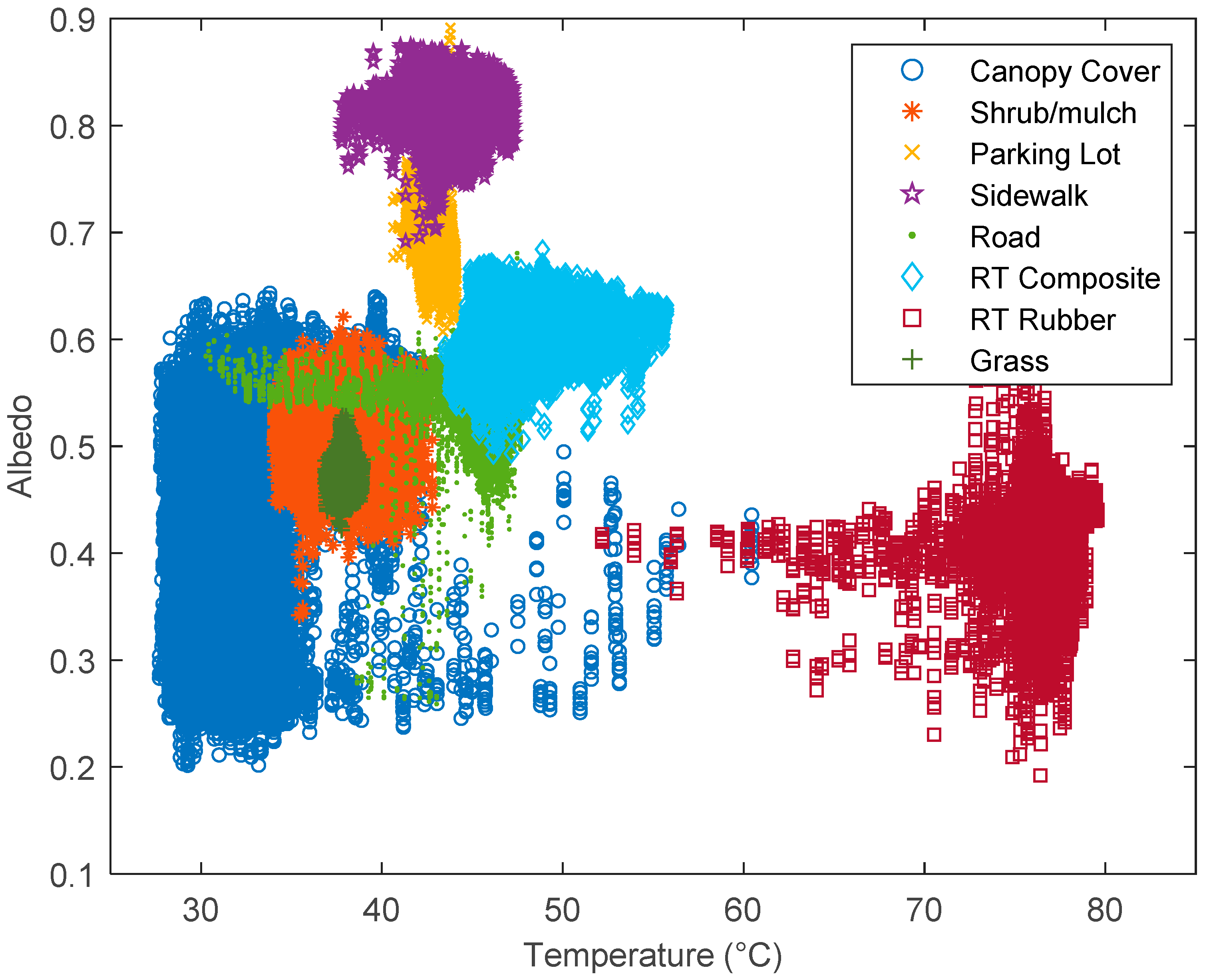
To further explore this variability and assess its impact on surface temperatures, we plotted these surface properties against land surface temperature. Figure 8 illustrates temperature plotted against its respective albedo for the 611,460 total data points captured by the drone imagery and results show clusters that form for different surface types. Some of these clusters exhibit either a (1) low range in albedo and high range in temperature or (2) high range in albedo and low range in temperature. For example, the road exhibits a low range in albedo and high range in temperature, implying the variability in roadway temperatures are more dependent on meteorological (e.g., exposure to solar radiation) and human (e.g., traffic) variables than physical properties (e.g., albedo). On the other hand, the parking lot has a higher but similar range in albedo, yet it has a much lower variability in temperature. This could be due to the fact that the parking lot has a range of materials from asphalt to concrete coupled with a much lower level of traffic as compared to the roadway, which is more homogenous and experiences constant vehicular traffic that intercepts land surface exposure to solar radiation. Therefore, this graphic may support the previous statement that there are anthropogenic variables, such as intermittent human foot or vehicular traffic, that are significant to land surface temperature processes. Overall these results suggest that patterns in the physical properties of urban materials may provide insight into surface temperature variability.
3.4. Temperature Prediction Models
Drone observations were applied to develop empirical models of land surface temperature. These include (1) a regression model to predict spatially averaged surface temperatures at 12:00 PM based upon environmental variables and (2) a diurnal model to predict surface temperatures throughout a given day.
3.4.1. Spatially Averaged Surface Temperature Regression Model
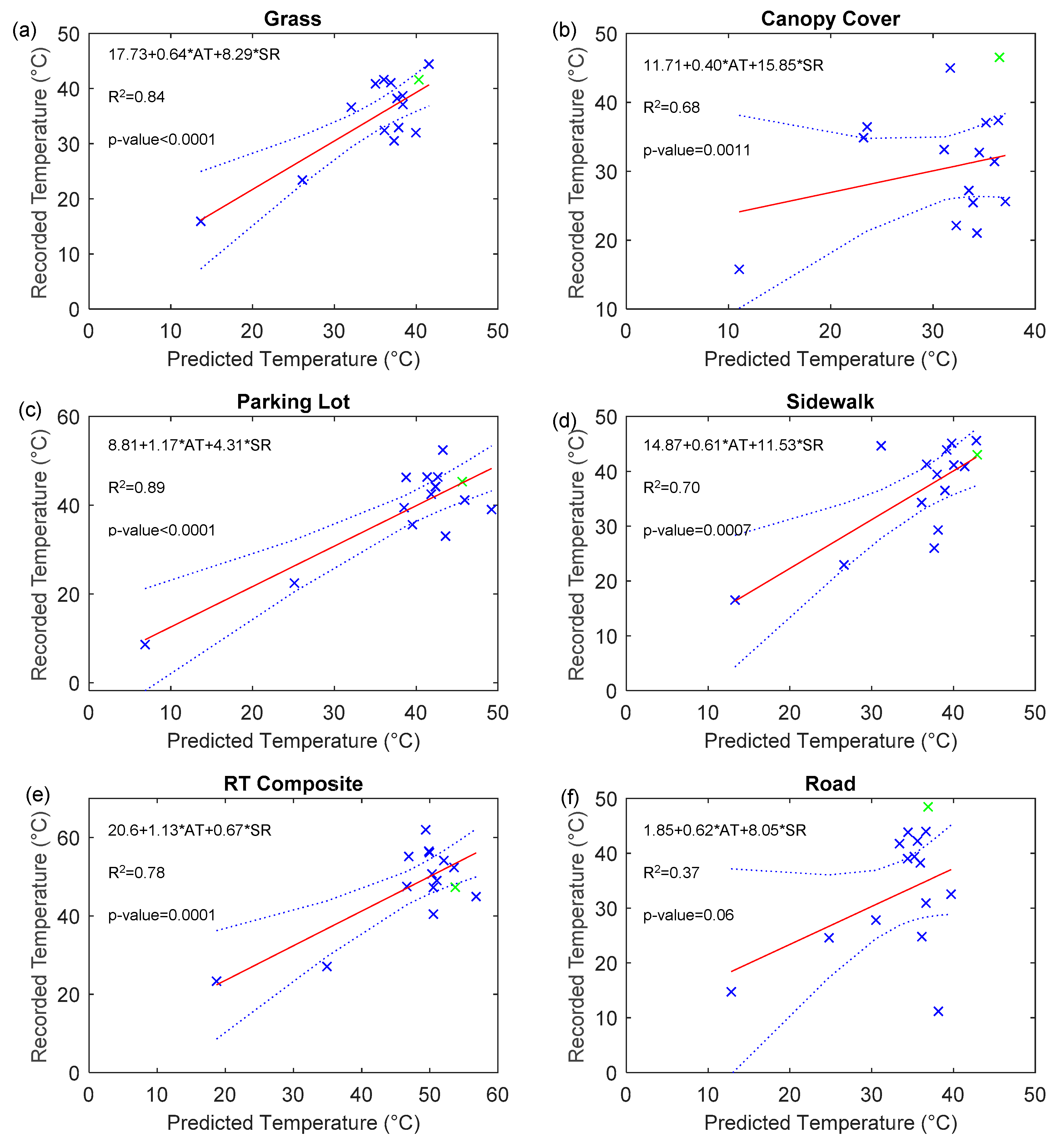
Multi-variable linear regression models were developed to predict spatially averaged surface temperature and it was found that air temperature and solar radiation are significant predictors (Figure 9). Standard least squares regression was applied to develop models that predict the surface temperature of six land use types: grass, canopy cover, parking lot (concrete), sidewalk, rooftop (composite) and road. The models had an average R2 of 0.71 with the parking lot having the greatest of (0.89) and the road the lowest (0.37). The parked cars and heat shadows were clipped out as inconsistencies before analysis occurred and therefore the parking lot surface had the most homogenous distribution of temperatures. The grass model had the second greatest R2 (0.84) and had a similarly homogenous distribution. Contrarily, the roadway surface had a much less homogenous distribution of temperatures and thus the road model had a low predictive power and statistical significance. This may be due in large part due to the difficulty of clipping out inconsistencies related to nonstationary objects (e.g., moving cars) combined with their impact on pavement temperatures.
The data collected in El Paso, TX was evaluated for influence and leverage and it was found that it did not have high influence or leverage in any of the six models. To evaluate influence we used Cook’s D and found that the El Paso data points all fell below the threshold of 2.4 (max 0.19) to be considered high-influence points [38]. In addition, we used the hat matrix to evaluate leverage and found that no El Paso data points exhibited high leverage in the model. The agreeability of the data across the two case study areas indicates that the findings in this study may have generalizability beyond the case study locations.
3.4.2. Diurnal Prediction Model
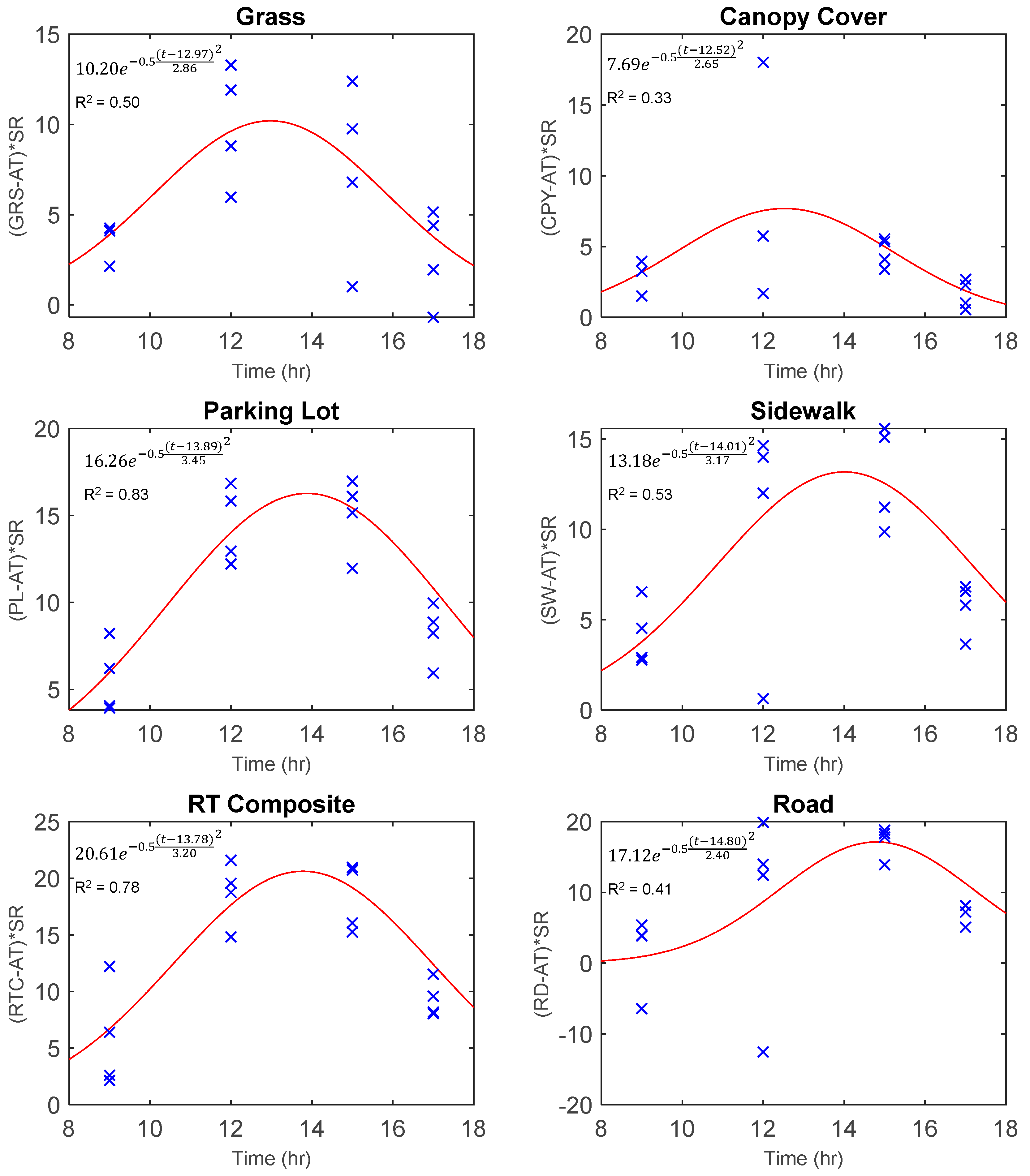
Finally, models were developed to predict land surface temperature throughout the day based upon the air temperature and solar radiation (Equations (7)–(9)). The diurnal data was fit with a Gaussian peak distribution and it was found that the parking lot and composite rooftop had the best model fit with an R2 of 0.83 and 0.78, respectively, while all other models had an R2 value of 0.53 or below (Figure 10). While this approach is constrained by a limited number of data points from four flights and only four numerical x-axis variables, there are a few insights we can gain from these results. The first is that these models confirm what was found in the previous regression models: it is much easier to predict the land surface temperature of homogenous materials, such as pavements and rooftops, than it is to predict land surfaces that have a greater distribution in texture and material, such as canopy. The second is that anthropogenic variables, such as pedestrians and vehicular traffic that are difficult to quantify, may influence the ability to predict surface temperatures based upon meteorological variables. This was shown by the lower model fit in the high-traffic roadways and sidewalks as compared to the low-traffic parking lot.
4. Discussion
We have presented a case study that applied high resolution drone measurements (13 cm) to evaluate urban surface temperatures and results indicate that there is a wide variability in surface temperature behavior across urban land use types. Some of the uncertainty in land surface temperature variability may be attributable to human movement patterns, land surface properties or urban geometry. Results indicate that mean land surface temperatures can be predicted based upon solar radiation and air temperature. By elucidating some of the factors that influence land surface temperature variability, we hope to contribute to the growing body of knowledge centered around land surface temperature in the urban environment.
To this end, our findings suggest that when parameterizing models, it is important to understand the unique relationship between surface material properties, urban geometry, weather and human movement. For example, the results indicate that pedestrian or vehicular traffic may have an impact on land surface temperature variability across sidewalks, parking lots and streets. Depending on the volume of cars, either parked or moving, this can greatly impact the temperature profile of paved surfaces. Parked cars can create heat shadows which cool the surface below and our study demonstrates that when a car moves it can reveal temperatures as low as 8.3 °C cooler than the exposed surface.
In addition, results have identified several factors of urban geometry that affect land surface temperatures. Urban factors such as building reflectivity and surface altitude can impact solar radiation, which then influences surface temperatures in locations impacted by these effects. For example, sidewalks often lie near buildings and depending on a buildings reflectance or shadows this can make sidewalk temperatures more vulnerable to temperature fluctuations. In this study, sidewalk temperatures impacted by glass reflectance were on average 4.7 °C hotter that sidewalks not impacted by reflectance. Therefore, knowledge of the spatial distribution of urban geometry is important for predicting and evaluating land surface temperatures in the built environment. While addressing urban geometry or pedestrian and vehicular traffic within our prediction models is outside of the scope of this project, future work should evaluate how to incorporate these important parameters into land surface temperature predictions.
Results indicate air temperature and solar radiation are significant predictors of mean land surface temperature in both of our models and it was found this relationship holds true in both Milwaukee, WI and El Paso, TX. Because the model holds true across two different climatic regions, the models developed in this project may be generalizable beyond their case study regions. In addition, these models can also be easily applied as air temperature and solar radiation are commonly measured across the world. The generalizability of these findings also has important implications for engineering applications that use predictions of land surface temperatures. Urban land surface temperatures are often used by public health officials to mitigate the impact of the urban heat island effect on human health [2], in developing binders and mixers of pavement in roadway designs [41] or to estimate the impact of land surface temperatures on receiving stream temperatures [42,43,44].
This study also demonstrates several advantages and disadvantages of using drones as compared to satellite or in-situ imagery. The case studies we evaluated were restricted to the size of a city block around 46,000 m2 and even though battery life would have allowed us to collect an area ten times this size, we were restricted by United States Federal Aviation Administration UAV pilot rules that restrict the flight of UAVs to within line of sight of the pilot. In an urban environment with tall buildings the line of sight may be the primary constraint on coverage area. Therefore, a disadvantage of UAVs is that flight time and legal restrictions may constrain the flight areas to small portions of a city. However, this could be overcome with fixed-wing drones that are able cover a greater area, in addition to relaxed regulations that allow flights beyond the line of sight [45]. Despite the restriction on the spatial extent of the study area, advantages of UAVs over satellites or in-situ methods are their ability to collect distributed temperature data at spatial resolutions (13 cm) that reflect small scale changes in the urban environment. In addition, satellite data is restricted to daily to weekly observations while drones can be flown on-demand, which allows them to capture temperature changes throughout the day.
Overall, this study highlights the utility of using drone observations to capture the variability of urban land surface temperatures at small spatial scales. Urban environments are spatially complex, making it difficult to capture the spatial distribution of observable phenomena outside of high-resolution remote sensing techniques. Our findings suggest that drones could also be good tools for evaluating the variability of other parameters of the urban environment that are important for environmental studies such as soil moisture, leaf area index or impervious cover. Therefore, it is important for studies such as this one that evaluate the spatial complexities of the urban environment in order to improve the methods that we use to model and understand urban systems.
5. Conclusions
The main objectives of this work were to apply drone imagery to capture land surface temperature variability and develop models to predict mean land surface temperatures. This was done through the application of high-resolution thermal imagery as a parameterizing tool for model development. The results revealed that land surface temperature variability is extensive and influenced by numerous variables related to urban environments and that air temperature and solar radiation are significant predictors of mean land surface temperature. Conclusions from this study hold true in both Milwaukee, WI and El Paso, TX, indicating they could be generalizable to regions beyond these two case study locations.
The key findings from this study were:
- Land surface variability was significant and ranged between (3.9–15.8 °C) for common land use types.
- Areas that experienced pedestrian or vehicular traffic exhibited higher variabilities than comparable surfaces that did not. In Milwaukee, the high-traffic road had a coefficient of variation of 0.32 as compared to 0.08 for the low-traffic parking lot. This indicates that human traffic may impact land surface temperatures due to the heat-shadow effect.
- Urban geometry has an influence on land surface temperatures; shadows and reflectance from buildings showed a significant influence on the temperatures of nearby land surfaces throughout the day. Sidewalk temperatures impacted by glass reflectance were on average 4.7 °C hotter that sidewalks not impacted by reflectance.
- Land surface temperature variability is low in the morning, peaks at noon and goes back down in the evening. This may indicate that as surfaces heat up, they do so at different rates, which contributes to more variability during mid-day.
- Air temperature and solar radiation were significant predictors of spatially averaged surface temperature in both of our models.
- Data were consistent in the models between Milwaukee, WI and El Paso, TX, suggesting that the findings in this study may be generalizable beyond the case study locations.
Overall, our findings suggest that land surface temperature variability in the urban environment can come from several sources including surface material properties, urban geometry, weather and pedestrian and vehicular traffic. This has direct implications for land surface temperature models that are used for urban environmental studies. As climate change and urbanization continue to exacerbate the SUHI, studies such as this are important for gaining a better understanding of the complexities of land surface temperatures. Ultimately this improved understanding will help to develop better methods and procedures to mitigate the impact of land surface temperatures on human and environmental health.
Author Contributions
J.N. provided investigation, data collection, data analysis, and writing of the original draft. W.M. contributed conceptualization, supervision, data collection and draft editing.
Funding
This project was funded by the Marquette OPUS College of Engineering Earl B. and Charlotte Nelson Award.
Acknowledgments
The authors would like to acknowledge and sincerely thank Saurav Kumar and Wissam Atwah at the University of Texas El Paso for their help in collecting data in El Paso, Tx.
Conflicts of Interest
The authors declare no conflict of interest.
References
- Foley, J.A.; DeFries, R.; Asner, G.P.; Barford, C.; Bonan, G.; Carpenter, S.R.; Chapin, F.S.; Coe, M.T.; Daily, G.C.; Gibbs, H.K.; et al. Global consequences of land use. Science 2005, 309, 570. [Google Scholar] [CrossRef] [PubMed]
- Shahmohamadi, P.; Che-Ani, A.I.; Etessam, I.; Maulud, K.N.A.; Tawil, N.M. Healthy Environment: The Need to Mitigate Urban Heat Island Effects on Human Health. Procedia Eng. 2011, 20, 61–70. [Google Scholar] [CrossRef] [Green Version]
- U.S. Environmental Protection Agency. The Assessment, Total Maximum Daily Load (TMDL) Tracking and Implementation System (ATTAINS); U.S. Environmental Protection Agency: Washington, DC, USA, 2019.
- White, P.A.; Kalff, J.; Rasmussen, J.B.; Gasol, J.M. The effect of temperature and algal biomass on bacterial production and specific growth rate in freshwater and marine habitats. Microb. Ecol. 1991, 21, 99–118. [Google Scholar] [CrossRef] [PubMed]
- Beitinger, T.L.; Bennett, W.A.; McCauley, R.W. Temperature Tolerances of North American Freshwater Fishes Exposed to Dynamic Changes in Temperature. Environ. Biol. Fishes 2000, 58, 237–275. [Google Scholar] [CrossRef]
- Lazzarini, M.; Marpu, P.R.; Ghedira, H. Temperature-land cover interactions: The inversion of urban heat island phenomenon in desert city areas. Remote Sens. Environ. 2013, 130, 136–152. [Google Scholar] [CrossRef]
- Jiang, Y.; Fu, P.; Weng, Q. Assessing the impacts of urbanization-associated land use/cover change on land surface temperature and surface moisture: A case study in the midwestern united states. Remote Sens. 2015, 7, 4880–4898. [Google Scholar] [CrossRef]
- Liu, L.; Zhang, Y. Urban heat island analysis using the landsat TM data and ASTER Data: A case study in Hong Kong. Remote Sens. 2011, 3, 1535–1552. [Google Scholar] [CrossRef]
- Sekertekin, A.; Kutoglu, S.H.; Kaya, S. Evaluation of spatio-temporal variability in Land Surface Temperature: A case study of Zonguldak, Turkey. Environ. Monit. Assess. 2016, 188, 1–15. [Google Scholar] [CrossRef]
- Sobrino, J.A.; Oltra-carrió, R.; Sòria, G.; Jiménez-muñoz, J.C.; Franch, B.; Hidalgo, V.; Mattar, C.; Julien, Y.; Cuenca, J.; Romaguera, M.; et al. Evaluation of the surface urban heat island effect in the city of Madrid. Int. J. Remote Sens. 2013, 34, 3177–3192. [Google Scholar] [CrossRef]
- Mallick, J.; Kant, Y.; Bharath, B.D. Estimation of land surface temperature over Delhi using Landsat-7 ETM+. J. Ind. Geophys. Union. 2008, 12, 131–140. [Google Scholar]
- Zhou, D.; Xiao, J.; Bonafoni, S.; Berger, C.; Deilami, K.; Zhou, Y.; Frolking, S.; Yao, R.; Qiao, Z.; Sobrino, J.A. Satellite Remote Sensing of Surface Urban Heat Islands: Progress, Challenges, and Perspectives. Remote Sens. 2018, 11, 48. [Google Scholar] [CrossRef]
- Granero-Belinchon, C.; Michel, A.; Lagouarde, J.-P.; Sobrino, J.A.; Briottet, X. Multi-Resolution Study of Thermal Unmixing Techniques over Madrid Urban Area: Case Study of TRISHNA Mission. Remote Sens. 2019, 11, 1251. [Google Scholar] [CrossRef]
- Nguyen, K.A.; Liou, Y.A. Global mapping of eco-environmental vulnerability from human and nature disturbances. Sci. Total Environ. 2019, 664, 995–1004. [Google Scholar] [CrossRef] [PubMed]
- Deng, C.; Wu, C. Estimating very high resolution urban surface temperature using a spectral unmixing and thermal mixing approach. Int. J. Appl. Earth Obs. Geoinf. 2013, 23, 155–164. [Google Scholar] [CrossRef]
- Nichol, J.E.; Wong, M.S. High resolution remote sensing of densely urbanised regions: A case study of Hong Kong. Sensors 2009, 9, 4695–4708. [Google Scholar] [CrossRef] [PubMed]
- Cooper, B.E.; Dymond, R.L.; Shao, Y. Impervious Comparison of NLCD versus a Detailed Dataset Over Time. Photogramm. Eng. Remote Sens. 2017, 83, 429–437. [Google Scholar] [CrossRef]
- Li, J.; Song, C.; Cao, L.; Zhu, F.; Meng, X.; Wu, J. Impacts of landscape structure on surface urban heat islands: A case study of Shanghai, China. Remote Sens. Environ. 2011, 115, 3249–3263. [Google Scholar] [CrossRef]
- Zhou, W.; Huang, G.; Cadenasso, M.L. Does spatial configuration matter? Understanding the effects of land cover pattern on land surface temperature in urban landscapes. Landsc. Urban Plan. 2011, 102, 54–63. [Google Scholar] [CrossRef]
- Chudnovsky, A.; Ben-Dor, E.; Saaroni, H. Diurnal thermal behavior of selected urban objects using remote sensing measurements. Energy Build. 2004, 36, 1063–1074. [Google Scholar] [CrossRef]
- Gaitani, N.; Burud, I.; Thiis, T.; Santamouris, M. High-resolution spectral mapping of urban thermal properties with Unmanned Aerial Vehicles. Build. Environ. 2017, 121, 215–224. [Google Scholar] [CrossRef]
- Kottek, M.; Grieser, J.; Beck, C.; Rudolf, B.; Rubel, F. World map of the Köppen-Geiger climate classification updated. Meteorol. Z. 2006, 15, 259–263. [Google Scholar] [CrossRef]
- National Weather Service Forcast Office. Available online: https://www.weather.gov/mkx/ (accessed on 17 July 2019).
- Marshall, S.J. We Need To Know More About Infrared Emissivity. Proc. SPIE 1982, 313, 119–128. [Google Scholar]
- Blonquist, J.M.; Norman, J.M.; Bugbee, B. Automated measurement of canopy stomatal conductance based on infrared temperature. Agric. For. Meteorol. 2009, 149, 1931–1945. [Google Scholar] [CrossRef]
- Humes, K.S.; Kustas, W.P.; Moran, M.S.; Nichols, W.D.; Weltz, M.A. Variability of emissivity and surface temperature over a sparsely vegetated surface. Water Resour. Res. 1994, 30, 1299–1310. [Google Scholar] [CrossRef]
- Wittich, K.P. Some simple relationships between land-surface emissivity, greenness and the plant cover fraction for use in satellite remote sensing. Int. J. Biometeorol. 1997, 41, 58–64. [Google Scholar] [CrossRef]
- Ramamurthy, P.; Bou-Zeid, E. Contribution of impervious surfaces to urban evaporation. Water Resour. Res. 2014, 50, 2889–2902. [Google Scholar] [CrossRef]
- Chen, H.; Ooka, R.; Huang, H.; Tsuchiya, T. Study on mitigation measures for outdoor thermal environment on present urban blocks in Tokyo using coupled simulation. Build. Environ. 2009, 44, 2290–2299. [Google Scholar] [CrossRef]
- Larsson, O.; Thelandersson, S. Estimating extreme values of thermal gradients in concrete structures. Mater. Struct. 2011, 44, 1491–1500. [Google Scholar] [CrossRef]
- Salamanca, F.; Krpo, A.; Martilli, A.; Clappier, A. A new building energy model coupled with an urban canopy parameterization for urban climate simulations—Part I. formulation, verification, and sensitivity analysis of the model. Theor. Appl. Climatol. 2009, 99, 331. [Google Scholar] [CrossRef]
- Herb, W.R.; Janke, B.; Mohseni, O.; Stefan, H.G. Thermal pollution of streams by runoff from paved surfaces. Hydrol. Process. 2008, 22, 987–999. [Google Scholar] [CrossRef]
- Spectrolab, Inc. Spectrolab Photovotaic Products Data Sheet; Spectrolab, Inc.: Sylmar, CA, USA, 2012. [Google Scholar]
- Ban-Weiss, G.A.; Woods, J.; Levinson, R. Using remote sensing to quantify albedo of roofs in seven California cities, Part 1: Methods. Sol. Energy 2015, 115, 777–790. [Google Scholar] [CrossRef] [Green Version]
- Carlson, T.N.; Ripley, D.A. On the relation between NDVI, fractional vegetation cover, and leaf area index. Remote Sens. Environ. 1997, 62, 241–252. [Google Scholar] [CrossRef]
- Sohrabinia, M.; Rack, W.; Zawar-Reza, P. Soil moisture derived using two apparent thermal inertia functions over Canterbury, New Zealand. J. Appl. Remote Sens. 2014, 8, 1–16. [Google Scholar]
- SAS Institute. JMP® 8 User Guide, 2nd ed.; SAS Institute Inc.: Cary, NC, USA, 2009. [Google Scholar]
- Helsel, D.R.; Hirsch, R.M. Statistical Methods in Water Resources; Elsevier: Amsterdam, The Netherlands, 2002; Volume 36. [Google Scholar]
- Thompson, A.M.; Wilson, T.; Norman, J.M.; Gemechu, A.L.; Roa-Espinosa, A. Modeling the effect of summertime heating on urban runoff temperature. J. Am. Water Resour. Assoc. 2008, 44, 1548–1563. [Google Scholar] [CrossRef]
- Guo, H. A Simple Algorithm for Fitting a Gaussian Function [DSP Tips and Tricks]. IEEE Signal Process. Mag. 2011, 28, 134–137. [Google Scholar] [CrossRef]
- Solaimanian, M.; Kennedy, T.W. Predicting Maximum Pavement Surface Temperature Using Maximum Air Temperature and Hourly Solar Radiation; Transportation Research Board: Washington, DC, USA, 1993. [Google Scholar]
- Herb, W.R.; Janke, B.; Mohseni, O.; Stefan, H.G. MINUHET (Minnesota Urban Heat Export Tool): A Software Tool for the Analysis of Stream Thermal Loading by Stormwater Runoff; Project Report No. 526; St. Anthony Falls Laboratory, The University of Minnesota: Minneapolis, MN, USA, 2009. [Google Scholar]
- Roa-Espinosa, A.; Wilson, T.B.; Norman, J.M.; Johnson, K. Predicting the Impact of Urban Development on Stream Temperature Using a Thermal Urban Runoff Model. Methods 2003, 369–389. [Google Scholar]
- Hailegeorgis, T.T.; Alfredsen, K. High spatial–temporal resolution and integrated surface and subsurface precipitation-runoff modelling for a small stormwater catchment. J. Hydrol. 2018, 557, 613–630. [Google Scholar] [CrossRef]
- Ravich, T. A Comparative Global Analysis of Drone Laws: Best Practices and Policies. In The Future of Drone Use: Opportunities and Threats from Ethical and Legal Perspectives; Custers, B., Ed.; T.M.C. Asser Press: The Hague, The Netherlands, 2016; pp. 301–322. ISBN 978-94-6265-132-6. [Google Scholar]
Figure 1.
Visual imagery of the case study locations: Marquette University (a) and University of Texas El Paso (UTEP) (b). Visual imagery of Marquette was captured from a drone on 11 August 2018. Visual imagery of UTEP was pulled from Google Maps on 13 March 2019.
Figure 1.
Visual imagery of the case study locations: Marquette University (a) and University of Texas El Paso (UTEP) (b). Visual imagery of Marquette was captured from a drone on 11 August 2018. Visual imagery of UTEP was pulled from Google Maps on 13 March 2019.

Figure 2.
Flow chart of data collection and processing.

Figure 3.
Boxplot distribution of surface temperature (a); and histogram of surface temperature (b). Data from flight recorded on July 11, 2018. Note GRS = grass; SM = shrub/mulch; CPY = canopy; PL = parking lot; SW = sidewalk; RTC = composite rooftop; RTR = rubber rooftop; RD = road; SLR = solar.
Figure 3.
Boxplot distribution of surface temperature (a); and histogram of surface temperature (b). Data from flight recorded on July 11, 2018. Note GRS = grass; SM = shrub/mulch; CPY = canopy; PL = parking lot; SW = sidewalk; RTC = composite rooftop; RTR = rubber rooftop; RD = road; SLR = solar.

Figure 4.
Boxplot distribution of average temperature, standard deviation and coefficient of variation from 14 recorded flights in Milwaukee, WI.
Figure 4.
Boxplot distribution of average temperature, standard deviation and coefficient of variation from 14 recorded flights in Milwaukee, WI.

Figure 5.
Standard deviation distributions for six land use types at hour 9, 12, 15 and 17 at both the MU and UTEP locations.
Figure 5.
Standard deviation distributions for six land use types at hour 9, 12, 15 and 17 at both the MU and UTEP locations.

Figure 6.
Spatial distribution of temperature from a flight recorded on 11 July 2018 (a) and zoomed in spatial distribution of temperature for the concrete parking lot from a flight recorded on 11 July 2018 (b). The hotter surfaces (red) in the right image are parked cars and the cooler surfaces (blue) are heat shadows visible after parked cars leave.

Figure 7.
Spatial distribution of tempearture (a), albedo (b), NDVI (c) and ATI (d) for a flight recorded on 11 August 2018.
Figure 7.
Spatial distribution of tempearture (a), albedo (b), NDVI (c) and ATI (d) for a flight recorded on 11 August 2018.

Figure 8.
Surface temperature data plotted against albedo from a flight recorded on 11 August 2018.

Figure 9.
Temperature prediction models of six surface types: grass (a), canopy cover (b), parking lot (c), sidewalk (d), composite rooftop (e) and road (f). UTEP datapoint is fitted in green. Note the 95% confidence intervals are in blue.
Figure 9.
Temperature prediction models of six surface types: grass (a), canopy cover (b), parking lot (c), sidewalk (d), composite rooftop (e) and road (f). UTEP datapoint is fitted in green. Note the 95% confidence intervals are in blue.

Figure 10.
Gaussian peak models of six surface types: grass (a), canopy cover (b), parking lot (c), sidewalk (d), composite rooftop (e) and road (f). Note that GRS = grass; CPY = canopy; PL = parking lot; SW = sidewalk; RTC = composite rooftop; AT = air temperature; SR = solar radiation; t = time.
Figure 10.
Gaussian peak models of six surface types: grass (a), canopy cover (b), parking lot (c), sidewalk (d), composite rooftop (e) and road (f). Note that GRS = grass; CPY = canopy; PL = parking lot; SW = sidewalk; RTC = composite rooftop; AT = air temperature; SR = solar radiation; t = time.


Table 1.
Surface types and surface areas within each case study location.
| MARQUETTE | UTEP | ||
|---|---|---|---|
| Surface Type | Surface Area (m2) | Surface Type | Surface Area (m2) |
| Grass | 2738 | Rooftop (rammed earth) | 503 |
| Sidewalk | 904 | Desert Shrub | 173 |
| Rooftop (composite) | 336 | Rooftop (composite) | 2047 |
| Road (asphalt) | 3299 | Parking Lot (asphalt) | 1350 |
| Parking Lot (concrete) | 908 | Sidewalk (concrete) | 9808 |
| Rooftop (rubber) | 6,057 | Road (asphalt) | 4253 |
| Canopy Cover | 4758 | Parking Lot (concrete) | 4081 |
| Shrub/mulch | 2272 | Grass | 1270 |
| Solar | 65 | Canopy Cover | 3782 |
Table 2.
Flight log and summary of meteorological variables recorded for Marquette and UTEP during fifteen noon flights.
Table 2.
Flight log and summary of meteorological variables recorded for Marquette and UTEP during fifteen noon flights.
| Flight Number | Flight Date | Flight Time | Air Temp (°C) | Relative Humidity (%) | Wind Speed (m/s) | Wind Dir (Degrees) | Solar Rad (kW/m2) | Pressure (kPa) |
|---|---|---|---|---|---|---|---|---|
| MU 1 | 26 February2018 | 12:00 PM | −1.7 | 54 | 4.0 | 225 | 0.00 | 102.2 |
| MU 2 | 12 April 2018 | 12:00 PM | 12.4 | 65.8 | 6.8 | 285 | 0.41 | 100.2 |
| MU 3 | 8 May 2018 | 12:00 PM | 26.4 | 22.1 | 4.2 | 218 | 0.81 | 101.7 |
| UTEP 1 | 20 May 2018 | 12:00 PM | 27.8 | 26 | 5.8 | 120 | 0.96 | 101.7 |
| MU 4 | 13 June 2018 | 12:00 PM | 25.3 | 33.3 | 3.4 | 321 | 0.89 | 101.2 |
| MU 5 | 29 June 2018 | 12:00 PM | 31.5 | 54.7 | 5.4 | 193 | 0.80 | 101.0 |
| MU 6 | 11 July 2018 | 12:00 PM | 25.9 | 44.1 | 2.0 | 91 | 0.78 | 101.9 |
| MU 7 | 12 July 2018 | 12:00 PM | 27.4 | 43.2 | 5.9 | 204 | 0.60 | 101.8 |
| MU 8 | 17 July 2018 | 12:00 PM | 25 | 38.9 | 3.0 | 38 | 0.74 | 101.6 |
| MU 9 | 18 July 2018 | 12:00 PM | 22.5 | 56.3 | 3.1 | 101 | 0.83 | 101.8 |
| MU 10 | 25 July 2018 | 12:00 PM | 28.6 | 31.9 | 2.5 | 271 | 0.83 | 101.4 |
| MU 11 | 10 August 2018 | 12:00 PM | 25.8 | 58.8 | 2.3 | 84 | 0.77 | 101.3 |
| MU 12 | 31 August 2018 | 12:00 PM | 25.8 | 49.9 | 4.0 | 158 | 0.09 | 101.6 |
| MU 13 | 12 September 2018 | 12:00 PM | 26.1 | 55.3 | 3.1 | 168 | 0.56 | 101.9 |
| MU 14 | 13 September 2018 | 12:00 PM | 22.8 | 64.9 | 4.2 | 127 | 0.68 | 102.0 |
Table 3.
Flight log and summary of meteorological variables recorded for Marquette and UTEP during four diurnal flights.
Table 3.
Flight log and summary of meteorological variables recorded for Marquette and UTEP during four diurnal flights.
| Flight Number | Flight Date | Flight Time | Air Temp (°C) | Relative Humidity (%) | Wind Speed (m/s) | Wind Dir (Degrees) | Solar Rad (kW/m2) | Pressure (kPa) |
|---|---|---|---|---|---|---|---|---|
| MU1 | 13 June 2018 | 9:00 AM | 22.5 | 42.8 | 4.4 | 320 | 0.73 | 101.1 |
| MU1 | 13 June 2018 | 12:00 PM | 25.3 | 33.3 | 3.4 | 321 | 0.89 | 101.2 |
| MU1 | 13 June 2018 | 3:00 PM | 27.5 | 20.1 | 3.0 | 328 | 0.80 | 101.2 |
| MU1 | 13 June 2018 | 5:00 PM | 27.9 | 19.8 | 2.0 | 285 | 0.51 | 101.2 |
| MU2 | 17 July 2018 | 9:00 AM | 23.8 | 37.7 | 3.1 | 8 | 0.52 | 101.6 |
| MU2 | 17 July 2018 | 12:00 PM | 25 | 38.9 | 3.0 | 38 | 0.74 | 101.6 |
| MU2 | 17 July 2018 | 3:00 PM | 25 | 41.2 | 3.0 | 38 | 0.76 | 101.7 |
| MU2 | 17 July 2018 | 5:00 PM | 22.8 | 57.9 | 3.4 | 34 | 0.50 | 101.7 |
| MU3 | 10 August 2018 | 9:00 AM | 27.4 | 46.1 | 2.4 | 33 | 0.70 | 101.3 |
| MU3 | 10 August 2018 | 12:00 PM | 25.7 | 58.8 | 2.3 | 84 | 0.77 | 101.3 |
| MU3 | 10 August 2018 | 3:00 PM | 27.4 | 46.1 | 2.4 | 33 | 0.70 | 101.3 |
| MU3 | 10 August 2018 | 5:00 PM | 27.4 | 33.4 | 2.4 | 37 | 0.43 | 101.2 |
| UTEP1 | 20 May 2018 | 9:00 AM | 25 | 32 | 5.8 | 90 | 0.66 | 101.8 |
| UTEP1 | 20 May 2018 | 12:00 PM | 27.8 | 26 | 5.8 | 120 | 0.96 | 101.7 |
| UTEP1 | 20 May 2018 | 3:00 PM | 31.1 | 17 | 4.0 | 120 | 0.83 | 101.4 |
| UTEP1 | 20 May 2018 | 5:00 PM | 31.1 | 21 | 4.9 | 90 | 0.50 | 101.3 |
Table 4.
Emissivity values for each surface type.
| Land Use Type | Emissivity Value | Reference |
|---|---|---|
| Grass | 0.979 | [26] |
| Shrub/mulch | 0.928 | [27] |
| Road (asphalt) | 0.95 | [28,29] |
| Parking Lot (concrete) | 0.91 | [29,30,31] |
| Sidewalk (concrete) | 0.91 | [24,29,30,31] |
| Rooftop (tar and stone) | 0.973 | [24] |
| Rooftop (black rubber) | 0.859 | [24] |
| Solar Panel | 0.85 | [32] |
| Canopy Cover | 0.977 | [33] |
Table 5.
Average temperature, standard deviation and coefficient of variation of nine surface types From 14 recorded flights on Marquette University campus and from one flight recorded on UTEP’s campus.
Table 5.
Average temperature, standard deviation and coefficient of variation of nine surface types From 14 recorded flights on Marquette University campus and from one flight recorded on UTEP’s campus.
| Location | Surface Type | Temp (°C) | Standard Dev (°C) | Coeff. of Variation |
|---|---|---|---|---|
| MU | Grass | 34.7 | 7.9 | 0.15 |
| Shrub/mulch | 40.7 | 6.2 | 0.12 | |
| Canopy | 30.4 | 7.2 | 0.16 | |
| Parking Lot | 38.7 | 4.2 | 0.08 | |
| Sidewalk | 36.3 | 11.2 | 0.21 | |
| Rooftop—Composite | 47.6 | 6.2 | 0.1 | |
| Rooftop—Rubber | 57.4 | 15.8 | 0.22 | |
| Road | 32.5 | 15.4 | 0.32 | |
| Solar Panels | 47.0 | 7.2 | 0.13 | |
| UTEP | Grass | 41.6 | 6.1 | 0.1 |
| Canopy | 46.6 | 6.3 | 10 | |
| Desert Shrub | 46.2 | 6.7 | 0.11 | |
| Parking Lot (asphalt) | 51.7 | 4.9 | 0.07 | |
| Parking (concrete) | 45.3 | 7.4 | 0.12 | |
| Sidewalk | 43.1 | 8.2 | 0.13 | |
| Rooftop—Composite | 47.3 | 7.2 | 0.11 | |
| Rooftop—Dzong | 46.2 | 6.3 | 0.1 | |
| Road | 48.4 | 2.8 | 0.04 |
Table 6.
Average albedo, normalized difference vegetation index (NDVI) and apparent thermal inertia (ATI) values for each surface type.
Table 6.
Average albedo, normalized difference vegetation index (NDVI) and apparent thermal inertia (ATI) values for each surface type.
| Surface Type | Albedo | NDVI | ATI |
|---|---|---|---|
| Grass | 0.317 | 0.369 | 0.198 |
| Shrub/mulch | 0.502 | 0.402 | 0.183 |
| Canopy | 0.378 | 0.490 | 0.209 |
| Parking Lot | 0.673 | 0.091 | 0.121 |
| Sidewalk | 0.472 | 0.144 | 0.195 |
| Rooftop–Composite | 0.580 | 0.101 | 0.156 |
| Rooftop–Rubber | 0.406 | 0.096 | 0.219 |
| Road | 0.518 | 0.117 | 0.179 |
| Solar | 0.333 | 0.143 | 0.217 |
© 2019 by the authors. Licensee MDPI, Basel, Switzerland. This article is an open access article distributed under the terms and conditions of the Creative Commons Attribution (CC BY) license (http://creativecommons.org/licenses/by/4.0/).
Share and Cite
MDPI and ACS Style
Naughton, J.; McDonald, W. Evaluating the Variability of Urban Land Surface Temperatures Using Drone Observations. Remote Sens. 2019, 11, 1722. https://0-doi-org.brum.beds.ac.uk/10.3390/rs11141722
AMA Style
Naughton J, McDonald W. Evaluating the Variability of Urban Land Surface Temperatures Using Drone Observations. Remote Sensing. 2019; 11(14):1722. https://0-doi-org.brum.beds.ac.uk/10.3390/rs11141722
Chicago/Turabian StyleNaughton, Joseph, and Walter McDonald. 2019. "Evaluating the Variability of Urban Land Surface Temperatures Using Drone Observations" Remote Sensing 11, no. 14: 1722. https://0-doi-org.brum.beds.ac.uk/10.3390/rs11141722
Note that from the first issue of 2016, this journal uses article numbers instead of page numbers. See further details here.