Deep Fully Convolutional Networks for Cadastral Boundary Detection from UAV Images


Faculty of Geo-Information Science and Earth Observation (ITC), University of Twente, 7522 NB Enschede, The Netherlands
*
Author to whom correspondence should be addressed.
Remote Sens. 2019, 11(14), 1725; https://0-doi-org.brum.beds.ac.uk/10.3390/rs11141725
Submission received: 12 June 2019
/
Revised: 17 July 2019
/
Accepted: 18 July 2019
/
Published: 20 July 2019
(This article belongs to the Special Issue Remote Sensing for Land Administration)
Abstract
:There is a growing demand for cheap and fast cadastral mapping methods to face the challenge of 70% global unregistered land rights. As traditional on-site field surveying is time-consuming and labor intensive, imagery-based cadastral mapping has in recent years been advocated by fit-for-purpose (FFP) land administration. However, owing to the semantic gap between the high-level cadastral boundary concept and low-level visual cues in the imagery, improving the accuracy of automatic boundary delineation remains a major challenge. In this research, we use imageries acquired by Unmanned Aerial Vehicles (UAV) to explore the potential of deep Fully Convolutional Networks (FCNs) for cadastral boundary detection in urban and semi-urban areas. We test the performance of FCNs against other state-of-the-art techniques, including Multi-Resolution Segmentation (MRS) and Globalized Probability of Boundary (gPb) in two case study sites in Rwanda. Experimental results show that FCNs outperformed MRS and gPb in both study areas and achieved an average accuracy of 0.79 in precision, 0.37 in recall and 0.50 in F-score. In conclusion, FCNs are able to effectively extract cadastral boundaries, especially when a large proportion of cadastral boundaries are visible. This automated method could minimize manual digitization and reduce field work, thus facilitating the current cadastral mapping and updating practices.
1. Introduction
Cadasters, which record the physical location and ownership of the real properties, are the basis of land administration systems [1]. Nowadays, cadastral mapping has received considerable critical attention. An effective cadastral system formalizes private property rights, which is very important to promote agricultural productivity, secure effective land market, reduce poverty and support national development in the broadest sense [2]. However, it is estimated that over 70% of the world population does not have access to a formal cadastral system [3]. Traditional field surveying approaches to record land parcels are often claimed to be time-consuming, costly and labor intensive. Therefore, there is a clear need for innovative tools to speed up this process.
Since the availability of very high resolution (VHR) satellite or aerial images, remote sensing has been used for mapping cadastral boundaries instead of field surveying, and is advocated by fit-for-purpose (FFP) land administration [4]. In practice, cadastral boundaries are often marked by physical objects, such as roads, building walls, fences, water drainages, ditches, rivers, clusters of stones, strips of uncultivated land, etc. [1]. Such boundaries are visible in remotely sensed images and bear the potential to be automatically extracted through image analysis algorithms, hence avoiding huge fieldwork surveying tasks. According to FFP, boundaries measured through on-site cadastral surveys using total station or the Global Navigation Satellite System (GNSS) with a precise location are considered as fixed, while boundaries delineated from high-resolution imagery are called general [4]. Although less spatially precise, general boundary approaches are much cheaper and faster than conventional cadastral surveys. Typically, high-resolution satellite images (HRSI) have been used for interpreting cadastral boundaries, but there are still obstacles such as high cost, cloudy or dated imagery [5]. Therefore, Unmanned Aerial Vehicles (UAV), renowned for low-cost and high spatial–temporal resolution, as well as being able to fly under clouds, are chosen as the data source for cadastral boundary extraction in this research.
The detection of cadastral boundaries from remotely sensed images is a difficult task. Above all, only visible cadastral boundaries coinciding with physical objects are detectable in the image. Moreover, as visible cadastral boundaries can be marked by different objects, spectral information alone is insufficient for the detection. In other words, there exists a sematic gap between the high-level boundary concept and low-level visual cues in the image. More reliable and informative features should be constructed to bridge the semantic gap, thus more advanced feature extraction techniques are needed.
State-of-the-art methods are mostly based on image segmentation and edge detection [6]. Segmentation refers to partitioning images into disjoint regions, inside which the pixels are similar to each other with regard to spectral characteristics [7]. Researchers claimed that segmentation-based approaches have two general drawbacks: Sensitive to intra-parcel variability and dependent on parameter selection. The latter often requires prior knowledge or trial and error [8]. Multi-Resolution Segmentation (MRS) is one of the most popular segmentation algorithms [9]. Classical edge detection aims to detect sharp changes in image brightness through local measurements, including first-order (e.g., Prewitt or Sobel) and second-order (e.g., Laplacian or Gaussian) derivative-based detection [10]. Derivative-based edge detection is simple but noise sensitive. Amongst others, the Canny detector is justified by many researchers as a predominant one, for its better performance and capacity to reduce noise [6]. More recently, learning-based edge detection stands out as remarkable progress, which combines multiple low-level image cues into statistical learning algorithms for edge response prediction [10]. Globalized Probability of Boundary (gPb) is considered as one of the state-of-the-art methods. It involves brightness, color and texture cues into a globalization framework using spectral clustering [11]. Both MRS and gPb are unsupervised techniques, hence the high-level cadastral boundary is still hard to distinguish from all the detected edges.
Recent studies indicate that deep learning methods such as Convolutional Neural Networks (CNNs) are highly effective for the extraction of higher-level representations needed for detection or classification from raw input [12], which brings in new opportunities in cadastral boundary detection. Traditional CNNs are usually made up of two main components, namely convolutional layers for extracting spatial-contextual features and fully connected feedforward networks for learning the classification rule [13]. CNNs follow a supervised learning algorithm. Large amounts of labeled examples are needed to train the network to minimize the cost function which measures the error between the output scores and the desired scores [14]. Fully Convolutional Networks (FCNs) are a more recent deep learning method. In an FCN architecture, the fully connected layers of traditional CNNs are replaced by transposed convolutions. This is the reason why these networks are called fully convolutional. As compared to CNNs, FCNs are able to perform pixel-wise predictions and accept arbitrary-sized input, thus largely reducing computational cost and processing time [15]. The superiority of FCNs in feature learning and computational efficiency makes them promising for the detection of visible cadastral boundaries, which provides the predominant motivation of this research. To the best of the authors’ knowledge, this is the first study investigating FCNs for cadastral boundary extraction.
In the remainder of this article, we apply deep FCNs for cadastral boundary detection based on UAV images acquired over one urban and one semi-urban area in Rwanda. We compare the results of FCNs with two other state-of-the-art image segmentation and edge detection techniques, namely MRS and gPb [9,11]. The performance of these methods is evaluated using the precision-recall framework. Specifically, to provide better insights into the detection results, we provide a separate accuracy assessment for visible and invisible cadastral boundaries, and an overall accuracy assessment for all cadastral boundaries.
2. Study Area
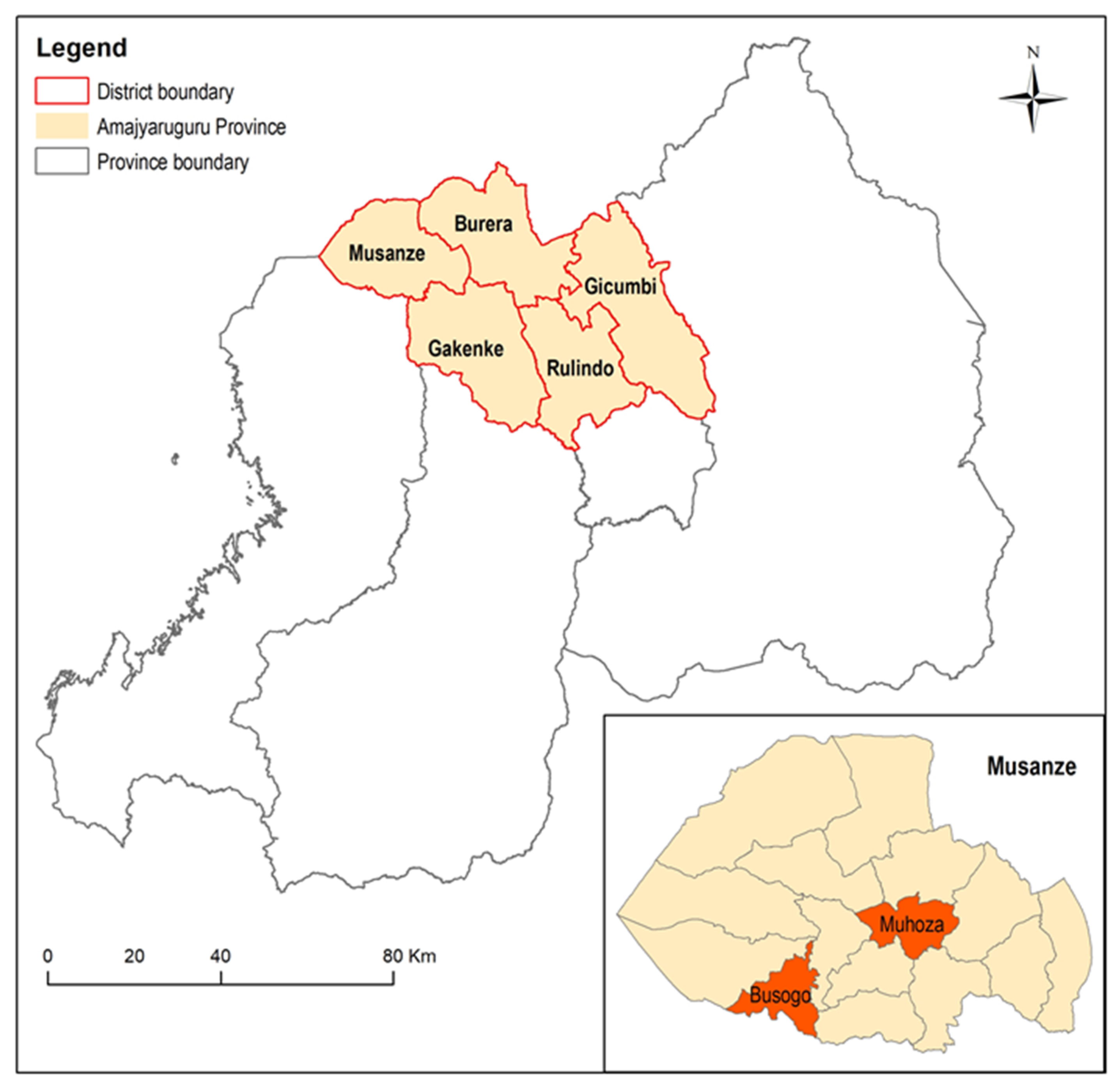
For the purpose of the study two sites within the Musanze district, Amajyaruguru Province of Rwanda, representing an urban and sub-urban setting, respectively, were selected as case-study locations. The selection is based on the availability of UAV images and the morphology of cadastral boundaries. The urban site is located in the Muhoza sector and the sub-urban site is in the Busogo sector. Figure 1 gives an overall view of the study area.
In 1962, land ownership in Rwanda had changed from customary law to a system of state ownership. In 2005, a new policy was accepted called Organic Land Law (OLL) with the aim to improve land tenure security. Rwanda is one of the countries which first tested the FFP approach. Since 2008, the country has been fully covered by aerial images acquired and processed by a Dutch company [16]. Even compromising with accuracy, Rwanda generated its national cadastral map based on these aerial images using a participatory mapping approach. However, due to the continuously changing environment, the data is currently outdated. New technologies supporting cheap, efficient and fit-for-purpose accurate cadastral mapping will largely facilitate the data updating practices in Rwanda. Therefore, the selection of the study area has been led by the impending local demand for data update.
3. Materials and Methods
The workflow of this research includes three major parts, namely data preparation, boundary detection and accuracy evaluation. In the first part, we selected three training tiles and one testing tile from each study area and prepared the RGB layer and boundary reference for each tile. In the second part, we applied FCNs, MRS and gPb for cadastral boundary detection and validated their performance based on the testing tiles. For the last part, we employed precision-recall measures for accuracy assessment, with a 0.4 m tolerance from reference data.
3.1. Data Preparation
The UAV images used in this research were acquired for the its4land (https://its4land.com/) project in Rwanda in 2018. All data collection flights were carried out by Charis UAS Ltd. The drone used for data collection in Busogo was a DJI Inspire 2, equipped with Zenmuse X5S sensor. The drone used in Muhoza was a FireFLY6 from BIRDSEYEVIEW, with a SONY A6000 sensor. Both sensors acquire three bands (RGB) and capture nadir images. The flight height above the ground for Busogo was 100 m and for Muhoza 90 m. The final Ground Sampling Distance (GSD) was 2.18 cm in Busogo and 2.15 cm in Muhoza. For more detailed information about flight planning and image acquisition refer to [17].
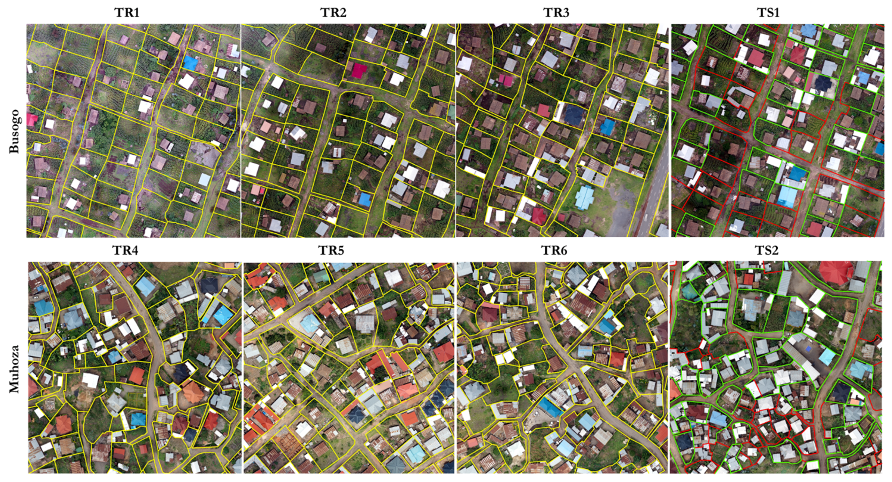
In this research, the spatial resolution of the UAV images was resampled from 0.02 m to 0.1 m considering the balance between accuracy and computational time. Four tiles of 2000 × 2000 pixels were selected from each study site for the experimental analysis. Among them, three tiles were used for training and one for testing the algorithm. The training and testing tiles in Busogo are named TR1, TR2, TR3 and TS1, and those in Muhoza are named TR4, TR5, TR6 and TS2 (Figure 2).
For each tile, RGB images and the boundary reference were prepared as input for the classification task. The reference data was acquired by merging the 2008 national cadaster and Rwandan experts’ digitization. The 2008 national cadaster is currently outdated, hence the experts’ digitization is provided as supplements. This acquired reference was presented as polygons in a shapefile format showing the land parcels. However, to feed the FCN, the boundary reference has to be in a raster format with the same spatial resolution as RGB images. Therefore, we first converted the polygons into borderlines and then rasterized the boundary lines with a spatial resolution of 0.1 m. Figure 2 visualizes the RGB images and boundary reference for the selected tiles in Busogo and Muhoza. To have a better understanding of the detection results on the testing tiles, we separated the boundary reference as visible and invisible in TS1 and TS2, which are marked as green and red in the above maps, respectively. We extracted visible cadastral boundaries by following clearly visible features, including strips of stones, fences, edge of the rooftop, road ridges, change in textural pattern and water drainage. Table 1 shows the rules that we followed for extracting visible boundaries in an extraction guide. The rest are considered invisible cadastral boundaries.
3.2. Boundary Detection
3.2.1. Fully Convolutional Networks
We address boundary detection as a supervised pixel-wise image classification problem to discriminate between boundary and non-boundary pixels. The network used in this research is modified from the FCN with dilated kernel (FCN-DK) as described in [18]. We mainly did three modifications: (1) discarding the max-pooling layers; (2) using smaller-size filters; and (3) constructing deeper networks. A typical max-pooling layer computes the local maximum within the pooling filter, thereby merging the information of nearby pixels and reducing the dimension of the feature map [14]. In most cases, down-sampling is performed using pooling layers to capture large spatial patterns in the image, and then the coarse feature maps extracted through this process are up-sampled back to produce pixel-wise prediction at the resolution of the input image. However, in the structure of FCN-DK, max-pooling layers are designed not to down-sample the input feature map by using a stride of one, therefore avoiding the need for up-sampling in the later stage. Nevertheless, the max-pooling results in a smoothing effect which is reducing the accuracy of boundaries. We therefore discarded it in the proposed network. In [18], Persello and Stein also demonstrated a case study based on FCN-DK using six convolutional layers with a filter size of 5 × 5 pixels. We modified it into 12 convolutional layers with 3 × 3 filters, as two 3 × 3 filters have the same receptive field as one 5 × 5 filter but less learnable parameters. Moreover, compared to single larger-sized filters, multiple small filters are interleaved by activation functions, resulting in better abstraction ability. Therefore, with less learnable parameters and better feature abstraction ability, smaller filters along with deeper networks are preferred.
Figure 3 shows the architecture of the proposed FCN. It consists of 12 convolutional layers interleaved by batch normalization and Leaky Rectified Linear Units (Leaky ReLU). Batch normalization layer is used to normalize each input mini-batch [19], and Leaky ReLU is the activation function of the network [20]. The classification is performed by the final SoftMax layer.
The core components of our network are the convolutional layers. They can extract spatial features hierarchically at different layers corresponding to different levels of abstraction. The 3 × 3 kernels used in the convolutional layers are dilated increasingly from 1 to 12 to capture larger contextual information. As a result, a receptive field of up to 157 × 157 pixels was achieved in the final layer. In each convolutional layer, zero paddings were used to keep the output feature maps at the same spatial dimension as the input. Therefore, the proposed FCN can be used to classify arbitrarily sized images directly and obtain correspondingly sized outputs.
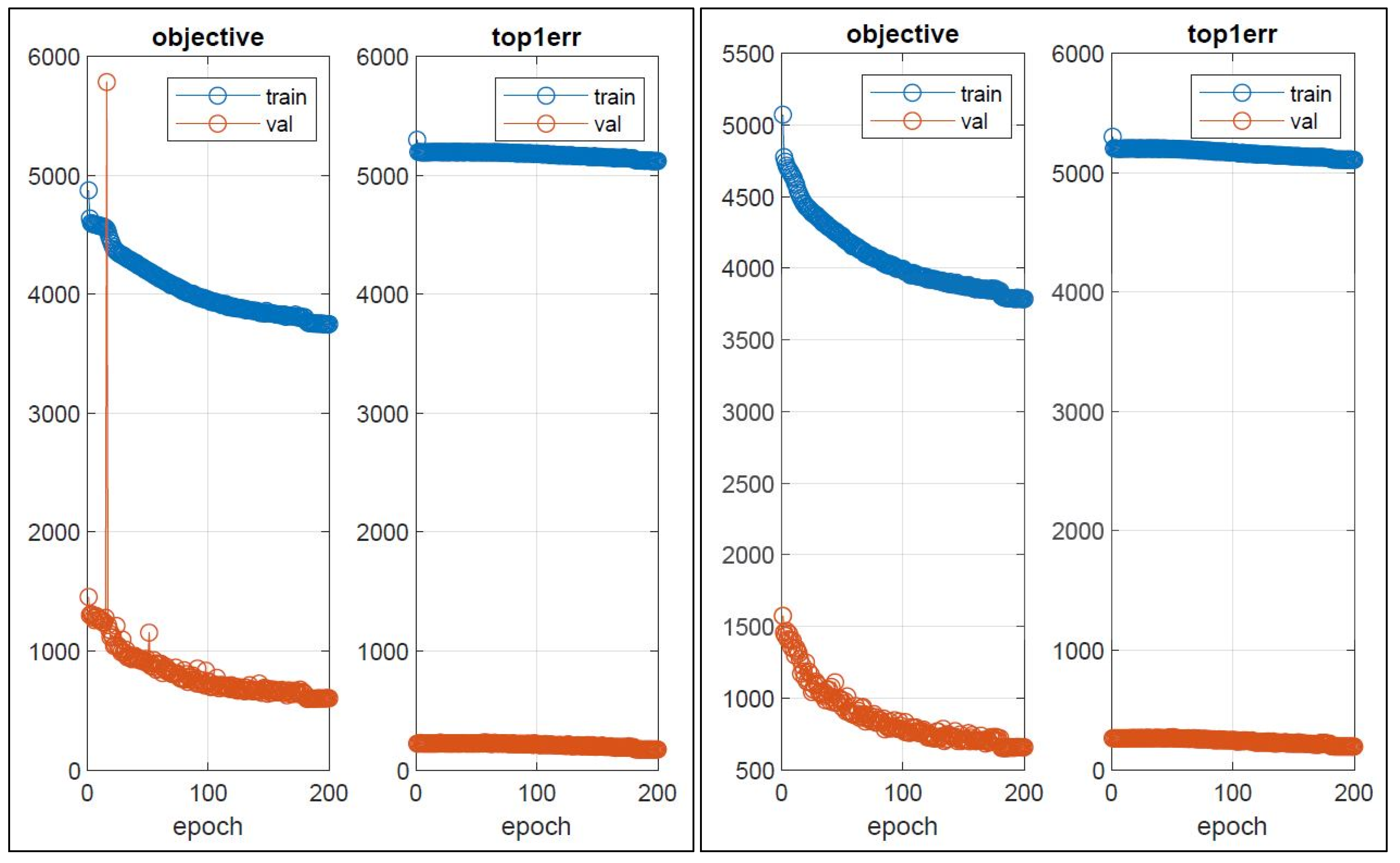
To train the FCN, we randomly extracted 500 patches for training and 500 patches for validation from each training tile. All the patches were fully labeled with a patch size of 145 × 145 pixels. Stochastic gradient descent with a momentum of 0.9 was used to optimize the loss function. The training is performed in multiple stages using a different learning rate. We use a learning rate of for the first 180 epochs and a learning rate of for another 20 epochs. A sudden decrease can be observed in the learning curves when the learning rate changes (Figure 4). The implementation of the network is based on the MatConvNet (http://www.vlfeat.org/matconvnet/) library. All experiments were performed on a desktop workstation with an Intel Core CPU i7-8750H at 2.2 GHz, 16 GB of RAM, and a Nvidia Quadro P1000 GPU. The training time for the FCN was 6 h for each study area.
3.2.2. Globalized Probability of Boundary (gPb)
Globalized Probability of Boundary (gPb) was proposed by Arbeláez et al. in 2011 [11]. gPb (global Pb) is a linear combination of mPb (multiscale Pb) and sPb (spectral Pb). The former conveys local multiscale Pb signals and the latter introduces global information. Multiscale Pb is an extension of the Pb detector advanced by Martin, Fowlkes and Malik [21]. The core block of Pb detector is calculating the oriented gradient signal (x,y,θ) from the intensity images. By placing a circular disc at the pixel location (x,) and dividing it into two half-discs at angle θ, we can obtain two histograms of pixel intensity values within each half-disc. (x,y,θ) is defined by the χ2 distance between the two histograms. For each input image, the Pb detector divides it into four intensity images, including brightness, color a, color b and texture channel. The oriented gradient signals are calculated separately for each channel. Multiscale Pb modifies the Pb detector by considering the gradients at three different scales, which means we give the discs three different diameters. Therefore, we can obtain local cues at different scales, from fine to coarse structures. For each pixel, the final mPb is obtained by combining the gradients of brightness, color a, color b and texture channel on three scales. Spectral Pb combines the multiscale image cues into an affinity matrix which defines the similarity between pixels. The eigenvectors of the affinity matrix which carry contour information are computed. They are treated as an image and convolved with Gaussian directional derivative filters. The sPb is calculated by combing the information from different eigenvectors.
Generally speaking, mPb detects all the edges while sPb extracts only the most salient one from the whole image. gPb combines the two and provides uniformly better performance. After detecting the boundary probability of each pixel using gPb, we also applied a grouping algorithm using the Oriented Watershed Transform and Ultrametric Contour Map (gPb–owt–ucm) to extract connected contours [11].
3.2.3. Multi-Resolution Segmentation (MRS)
We conducted MRS in eCognition software (version 9.4). MRS is a region-merging technique starting from each pixel forming one image object or region [22,23]. The merging criteria is local homogeneity, which describes the similarity between adjacent image objects. The merging procedure stops when all the possible merges exceed the homogeneity criteria.
MRS relies on several parameters, which are image layer weights, scale parameter (SP), shape and compactness. Image layer weights define the importance of each image layer to the segmentation process. In this research, we had three layers (RGB) in the input image. We gave them equal weights. Scale parameter is the most important parameter, which controls the average image object size [9]. A larger scale parameter allows higher spectral heterogeneity within the image objects, hence allowing more pixels within one object. Defining the proper SP is critical for MRS. In our research, we selected the SP resorting to the automatic Estimation of Scale Parameters 2 (ESP2) tool, which was advanced in [9]. Shape parameter ranges from 0 to 1. It indicates a weighting between the object’s shape and its spectral color. A high value in shape parameter means less importance is put on spectral information. We set a shape parameter of 0.3 in our research. Compactness defines how compact the segmented objects are. The higher the value, the more compact the image objects may be. It was set to 0.5 in this research.
3.3. Accuracy Assessment
The results in this research were evaluated considering the detection accuracy on the testing tiles. While validating the predicted results with reference data, a certain tolerance is often used in cadastral mapping. According to the International Association of Assessing Officers (IAAO), the horizontal spatial accuracy for cadastral maps in urban environments is usually 0.3 m or less, and in rural areas an accuracy of 2.4 m is sufficient [24]. Besides, FFP approaches advocates the flexibility in terms of accuracy to best accommodate social needs [3]. Complying with FFP land administration, we chose a 0.4 m tolerance for urban and peri-urban environments in this research. When adopted for other applications, this number can be adjusted correspondingly and according to the demands.
The accuracy assessment resorted to precision-recall measures, which are a standard evaluation technique especially for boundary detection in computer vision fields [21]. Precision (P), also called correctness, measures the ratio of correctly detected boundary pixels to the total detected boundary pixels. Recall (R), also called completeness, indicates the percentage of correctly detected boundaries to the total boundaries in the reference. The F measure (F) represents the harmonic mean between precision and recall [25]. As F combines both precision and recall, it can be regarded as an overall quality measure. The range of these three measures is between 0 and 1. Larger values represent higher accuracy.
Specifically, the accuracy assessment was done by overlapping the detected boundary with buffered reference data (0.4 m buffer). With the following table and formulas, we indicated how to calculate precision, recall and the F-score. Pixels labelled as boundary class in both detection and the buffered reference are called True Positive (TP), while pixels labelled as boundary in detection but non-boundary in the buffered reference are called False Positive (FP). The term False Negative (FN) and True Negative (TN) are defined similarly (Table 2). By overlaying the detection result with the buffered reference, we can obtain the value of TP, FP, TN and FN, respectively. TP stands for the number of correctly detected boundary pixels, and the sum of TP and FP indicates the number of total detected boundary pixels. Hence, we can calculate the value of precision through Formula 1. However, the sum of TP and FN stands for the number of total boundaries in the buffered reference, rather than the original reference. Therefore, we need to divide the sum of TP and FN by 8, which is the width of the buffered reference, to get the number of total boundaries in the original reference. This is because the buffered reference has a uniform width of 8 pixels, while the original reference is only single-pixel wide. Equations (2) and (3) show how to calculate recall and the F-score.
In order to know the capability of different methods in detecting visible and invisible cadastral boundaries, we calculated the classification accuracy for the visible cadastral boundary, invisible cadastral boundary and all cadastral boundaries, separately. By overlapping the detected boundary with the buffered reference of only visible, invisible or all cadastral boundaries, we obtain three sets of accuracy assessment results for each algorithm on every testing tile.
4. Results
The proposed method along with the competing methods were implemented on both study sites, Busogo and Muhoza, to test their generalization ability. The results are evaluated considering the classification accuracy on the testing tiles using the precision-recall framework. The visual and numerical results of the testing tiles are demonstrated in the following table and figures.
Table 3 presents the separate accuracy for visible and invisible boundaries, as well as the overall accuracy for all cadastral boundaries of each algorithm on TS1 and TS2. Taking the classification accuracy of FCN on visible cadastral boundaries in TS1 as an example, FCN achieves 0.75 in precision, which means the ratio of truly detected visible boundaries to the total detected boundaries is 75%. The value of recall is 0.65, indicating 65% of visible cadastral boundaries among all the visible boundaries in the reference are detected. The final F-score of FCN is 0.70, which can be regarded as an overall measure of quality performance. Other results from Table 3 could be interpreted in the same way. Interestingly, according to the mathematical implications of precision, the sum of the P value on visible and invisible boundaries should be equal to the P value on all cadastral boundaries. We can easily verify this through the six sets of data in Table 3, with a small tolerance of .
According to Table 3, FCN achieves an F-score of 0.70 on visible boundaries and 0.06 on invisible boundaries in TS1. The score of the former is much higher than the latter. A similar situation can also be witnessed in TS2, which indicates that FCN detects mainly visible cadastral boundaries. The F-score of FCN on all boundaries in TS1 is 0.52, larger than that in TS2 (0.48). We can interpret this result considering the proportion of visible cadastral boundaries (The proportion of visible cadastral boundaries in each tile are calculated by computing the ratio of the total length of visible cadastral boundaries to that of all cadastral boundaries) in each tile, which is 57% in TS1 and 72% in TS2. Surprisingly, with more visible cadastral boundaries, TS2 get poorer detection results. According to the R value of visible boundaries, 65% of visible cadastral boundaries are detected in TS1 and the number is only 45% in TS2. It means that although TS2 has more visible cadastral boundaries, less of them are detected. The main difference in detection ability of the FCN in TS1 and TS2 can be understood by considering the various types of visible cadastral boundaries. TS1 is located in a sub-urban area, with fences and strips of stones being the most predominant visible boundaries, whereas TS2 is in an urban area, where building walls and fences play the leading role. The better performance of FCN in TS1 indicates that FCN is good in detecting visible boundaries like fences and strips of stones, while cadastral boundaries that coincide with building walls are more difficult for FCN to recognize. Based on the above analysis we can conclude that FCN detects mainly visible cadastral boundaries, especially those demarcated by fences or strips of stones.
Comparing FCN to gPb–owt–ucm and MRS, the most salient finding is that under the same situation, like the detection accuracy for visible boundary in TS1 or all boundaries in TS2, the P value of FCN is always larger than that of gPb–owt–ucm and MRS, while the R value of FCN is always smaller. FCN always achieves the highest F-score. These results show that gPb–owt–ucm and MRS can detect large proportion of cadastral boundaries, but also many false boundaries. FCN has a very high precision rate, leading to the best overall performance.
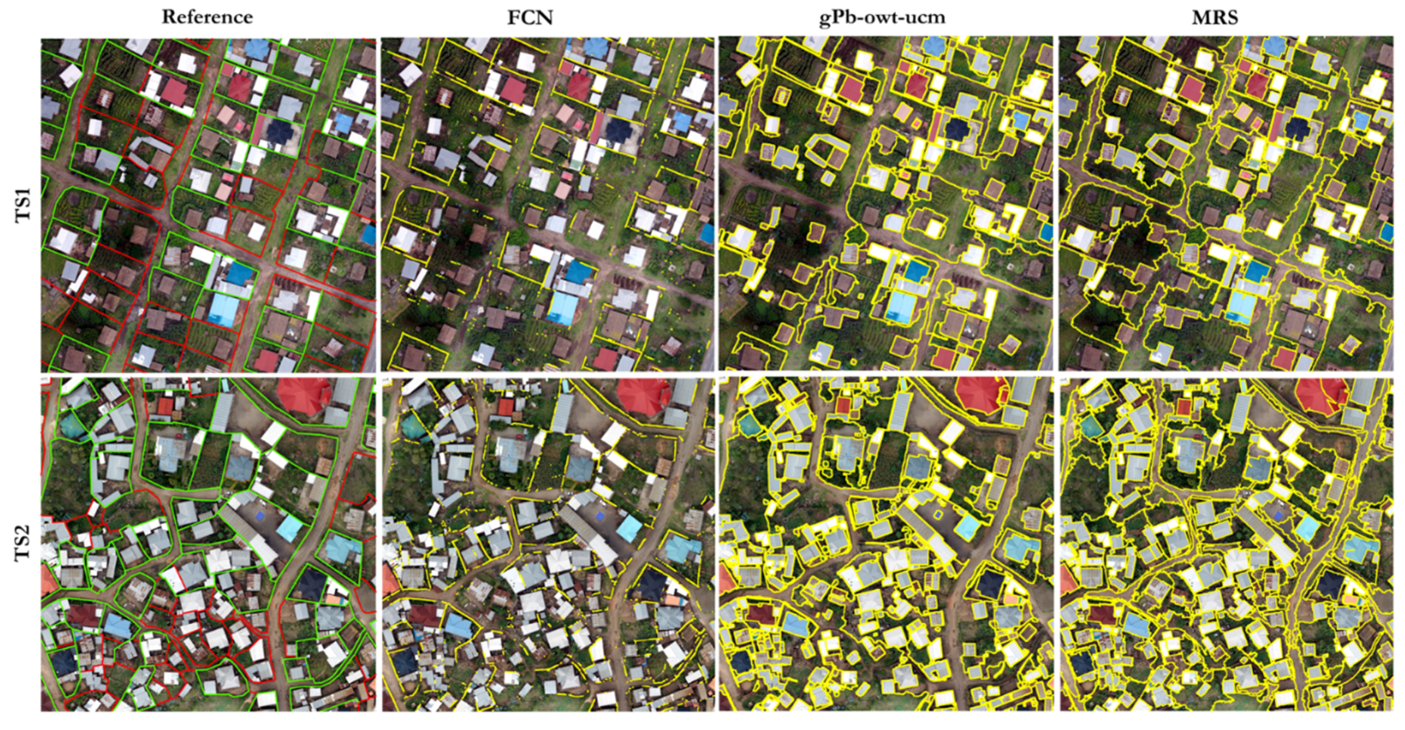
Figure 5 shows the visible and invisible boundary references and the detected results of the investigated algorithms. According to Figure 5, the missing boundary fragments in the FCN classification output are mainly invisible boundaries. Besides, FCN has a more regular and cleaner output than gPb–owt–ucm and MRS. Although the outlines of buildings and trees correspond to strong edges, they are not confused by FCN with cadastral boundaries.
Figure 6 presents the error map of the detection results. By overlapping the detection map with the boundary reference, the correctly detected boundaries are marked as yellow; the false detection rea marked as red; and the missing boundaries are marked as green. Figure 6 supplies a better intuition of the detection results. Fewer red lines can be observed in the FCN output as compared to the other two algorithms, once again proving that FCN has higher precision.
The difference in computational cost between these methods is also worth highlighting. As mentioned earlier, it takes 6 h to train the FCN. However, once trained well, one tile is classified in 1 min with the proposed FCN, whereas it takes 38 min for MRS and 1.5 h for gPb–owt–ucm, respectively.
5. Discussion
Considering the constraints of the invisible cadastral boundaries, land administration professionals perceived that a 40 to 50 percent automatic delineation would be very significant in reducing time and labor involved in cadastral mapping practices [26]. This goal is reached by FCN with a 0.4 m tolerance in both Busogo and Muhoza, indicating good generalization and transferability of the proposed approach in cadastral boundary mapping. From Section 4, the numerical results and visual results proves and supplements each other, suggesting two main findings: (1) The true positives detected by the FCN are mainly visible boundaries like fences and strips of stones; and (2) gPb–owt–ucm and MRS have high recall, while FCN has high precision and better overall performance.
Compared with alternative edge detection and image segmentation approaches, FCN achieved better overall performance. The reason lies in the strong feature learning and abstraction ability of FCN. Lacking abstraction ability, standard edge detection and image segmentation cannot fill the semantic gap between the high-level cadastral boundary concept and low-level image features. As a result, gPb–owt–ucm and MRS achieved high recall but low precision. In other words, gPb–owt–ucm cannot determine cadastral boundaries from all the detected contours, while MRS cannot eliminate over-segmentation caused by the spectral differences within one cadastral parcel. It is also worth noticing that FCN performs supervised boundary detection, while MRS and gPb–owt–ucm are both unsupervised techniques. This may explain their differences in the abstraction ability. Being supervised, the proposed FCN-based detector is trained to detect cadastral boundaries and to disregard other irrelevant edges like building outlines.
FCN can supply high precision, while gPb–owt–ucm and MRS can supply high recall. Therefore, for further study, we can consider a combination of these methods. We can combine them in two ways. The first one is to involve the output of gPb or MRS along with UAV images as input for FCN. FCN has a strong feature learning ability. It is possible that FCN can determine cadastral boundaries from the outputs of gPb or MRS, hence increasing both precision and recall. The second way is to apply an approach similar to [27], where the boundary map of FCN and the probability map of gPb are linearly combined and followed by the owt–ucm procedure to extract connected boundaries.
6. Conclusions
The deep FCN proposed in this research is capable of extracting visible cadastral boundaries from raw UAV images. Experiments carried out on both study sites achieved an F-score around 0.5. Very clean and clear boundaries were extracted by the proposed method, avoiding the effect of messy building contours. In both study sites, the proposed method performed better than contending algorithms. The knowledge of the local experts is needed to correct the extracted boundaries and include them in a final cadastral system. We conclude that the proposed automated method followed by experts’ final correction and verification can reduce the processing time and labor force of the current cadastral mapping and data updating practices.
So far, the proposed technique is mainly suitable when a large proportion of boundaries are visible. Detecting invisible boundaries, i.e., not demarcated by physical objects, from remotely sensed images is obviously extremely challenging. In other researches, invisible boundaries are identified by manual digitization via post-processing steps. The its4land project proposed a QGIS plugin (https://its4land.com/automate-it-wp5/) which supports an interactive, semi-automatic delineation to expedite the process. In the beginning of this research, the authors also attempted to fill this research gap by considering the fact that a cadastral boundary often lies in between two buildings. We tried to introduce building information as an additional input to train the FCNs for identifying the invisible boundaries. However, our experimental results obtained so far showed that there was no obvious improvement by adding building information in cadastral boundary detection. Further research is required in this direction. In future research, we will consider to improve the capability to detect cadastral boundaries (visible and invisible) using Generative Adversarial Networks (GANs) [28]. Within this framework, the generative model and discriminative model form an adversarial training, which is sharpening the training process by focusing on the most critical samples to learn. This approach is expected to improve the accuracy in boundary detection tasks which are often characterized by scarce training data.
Author Contributions
M.K., C.P., and X.X. conceptualized the aim of this research; X.X. wrote the majority of the paper; C.P. and M.K revised and edited the paper over several rounds; and X.X. set up and performed the experimental analysis using parts of the software codes developed by C.P. and under the supervision of both C.P. and M.K.
Funding
This research received no external funding.
Acknowledgments
The authors would like to thank the team of “its4land” research project number 687828 which is part of the Horizon 2020 program of the European Union, for providing UAV data for this research.
Conflicts of Interest
The authors declare no conflict of interest.
References
- Luo, X.; Bennett, R.M.; Koeva, M.; Lemmen, C. Investigating Semi-Automated Cadastral Boundaries Extraction from Airborne Laser Scanned Data. Land 2017, 6, 60. [Google Scholar] [CrossRef]
- Williamson, I. The justification of cadastral systems in developing countries. Geomatica 1997, 51, 21–36. [Google Scholar]
- Enemark, S.; Mclaren, R.; Lemmen, C.; Antonio, D.; Gitau, J.; De Zeeuw, K.; Dijkstra, P.; Quinlan, V.; Freccia, S. Fit-For-Purpoes Land Administration: Guiding Principles for Country Implementation; GLTN: Nairobi, Kenya, 2016. [Google Scholar]
- Enemark, S.; Bell, K.C.; Lemmen, C.; McLaren, R. Fit-For-Purpose Land Administration; International Federation of Surveyors: Copenhagen, Denmark, 2014; p. 44. [Google Scholar]
- Ramadhani, S.A.; Bennett, R.M.; Nex, F.C. Exploring UAV in Indonesian cadastral boundary data acquisition. Earth Sci. Inform. 2018, 11, 129–146. [Google Scholar] [CrossRef]
- Crommelinck, S.; Bennett, R.; Gerke, M.; Nex, F.; Yang, M.; Vosselman, G. Review of Automatic Feature Extraction from High-Resolution Optical Sensor Data for UAV-Based Cadastral Mapping. Remote Sens. 2016, 8, 689. [Google Scholar] [CrossRef]
- Pal, N.R.; Pal, S.K. A review on image segmentation techniques. Pattern Recognit. 1993, 26, 1277–1294. [Google Scholar] [CrossRef]
- García-Pedrero, A.; Gonzalo-Martín, C.; Lillo-Saavedra, M. A machine learning approach for agricultural parcel delineation through agglomerative segmentation. Int. J. Remote Sens. 2017, 38, 1809–1819. [Google Scholar] [CrossRef] [Green Version]
- Drǎguţ, L.; Csillik, O.; Eisank, C.; Tiede, D. Automated parameterisation for multi-scale image segmentation on multiple layers. ISPRS J. Photogramm. Remote Sens. 2014, 88, 119–127. [Google Scholar] [CrossRef] [PubMed]
- Li, Y.; Wang, S.; Tian, Q.; Ding, X. A survey of recent advances in visual feature detection. Neurocomputing 2015, 149, 736–751. [Google Scholar] [CrossRef]
- Arbeláez, P.; Maire, M.; Fowlkes, C.; Malik, J. Contour Detection and Hierarchical Image Segmentation. IEEE Trans. Pattern Anal. Mach. Intell. 2011, 33, 898–916. [Google Scholar] [CrossRef] [PubMed]
- Zhu, X.X.; Tuia, D.; Mou, L.; Xia, G.-S.; Zhang, L.; Xu, F.; Fraundorfer, F. Deep Learning in Remote Sensing: A Comprehensive Review and List of Resources. IEEE Geosci. Remote Sens. Mag. 2017, 5, 8–36. [Google Scholar] [CrossRef] [Green Version]
- Bergado, J.R.; Persello, C.; Gevaert, C. A Deep Learning Approach to the Classification of sub-decimetre Resolution Aerial Images. In Proceedings of the IEEE International Geoscience and Remote Sensing Symposium, Beijing, China, 10–15 July 2016; pp. 1516–1519. [Google Scholar]
- LeCun, Y.; Bengio, Y.; Hinton, G. Deep learning. Nature 2015, 521, 436–444. [Google Scholar] [CrossRef] [PubMed]
- Shelhamer, E.; Long, J.; Darrell, T. Fully Convolutional Networks for Semantic Segmentation. IEEE Trans. Pattern Anal. Mach. Intell. 2017, 39, 640–651. [Google Scholar] [CrossRef] [PubMed]
- Maurice, M.J.; Koeva, M.N.; Gerke, M.; Nex, F.; Gevaert, C. A photogrammetric approach for map updating using UAV in Rwanda. In Proceedings of the GeoTechRwanda 2015, Kigali, Rwanda, 18–20 November 2015; pp. 1–8. [Google Scholar]
- Stöcker, C.; Ho, S.; Nkerabigwi, P.; Schmidt, C.; Koeva, M.; Bennett, R.; Zevenbergen, J. Unmanned Aerial System Imagery, Land Data and User Needs: A Socio-Technical Assessment in Rwanda. Remote Sens. 2019, 11, 1035. [Google Scholar] [CrossRef]
- Persello, C.; Stein, A. Deep Fully Convolutional Networks for the Detection of Informal Settlements in VHR Images. IEEE Geosci. Remote Sens. Lett. 2017, 14, 2325–2329. [Google Scholar] [CrossRef] [Green Version]
- Ioffe, S.; Szegedy, C. Batch Normalization: Accelerating Deep Network Training by Reducing Internal Covariate Shift. In Proceedings of the International Conference on Machine Learning, Lille, France, 6–11 July 2015. [Google Scholar]
- He, K.; Zhang, X.; Ren, S.; Sun, J. Delving Deep into Rectifiers: Surpassing Human-Level Performance on ImageNet Classification. In Proceedings of the 2015 IEEE International Conference on Computer Vision (ICCV), Santiago, Chile, 7–13 December 2015; pp. 1–11. [Google Scholar] [CrossRef]
- Martin, D.R.; Fowlkes, C.C.; Malik, J. Learning to detect natural image boundaries using local brightness, color, and texture cues. IEEE Trans. Pattern Anal. Mach. Intell. 2004, 26, 530–549. [Google Scholar] [CrossRef] [PubMed]
- Baatz, M.; Schäpe, A. Multiresolution Segmentation: An Optimization Approach for High Quality Multi-Scale Image Segmentation; Wichmann Verlag: Karlsruhe, Germany, 2000. [Google Scholar]
- Nyandwi, E.; Koeva, M.; Kohli, D.; Bennett, R.; Nyandwi, E.; Koeva, M.; Kohli, D.; Bennett, R. Comparing Human Versus Machine-Driven Cadastral Boundary Feature Extraction. Remote Sens. 2019, 11, 1662. [Google Scholar] [CrossRef]
- IAAO. Standard on Digital Cadastral Maps and Parcel Identifiers; International Association of Assessing Officers: Kansas City, MO, USA, 2015. [Google Scholar]
- Hossin, M.; Sulaiman, M.N. Review on Evaluation Metrics for Data Classification Evaluations. Int. J. Data Min. Knowl. Manag. Process 2015, 5, 1–11. [Google Scholar] [CrossRef]
- Wassie, Y.A.; Koeva, M.N.; Bennett, R.M.; Lemmen, C.H.J. A procedure for semi-automated cadastral boundary feature extraction from high-resolution satellite imagery. J. Spat. Sci. 2018, 63, 75–92. [Google Scholar] [CrossRef]
- Persello, C.; Tolpekin, V.A.; Bergado, J.R.; de By, R.A. Delineation of agricultural fields in smallholder farms from satellite images using fully convolutional networks and combinatorial grouping. Remote Sens. Environ. 2019, 231, 111253. [Google Scholar] [CrossRef]
- Goodfellow, I.J.; Pouget-Abadie, J.; Mirza, M.; Xu, B.; Warde-Farley, D.; Ozair, S.; Courville, A.; Bengio, Y. Generative Adversarial Networks. In Proceedings of the Neural Information Processing Systems, Montreal, QC, Canada, 8–13 December 2014; pp. 2672–2680. [Google Scholar]
Figure 1.
Study areas. Two case study sites in Rwanda were selected, namely Busogo and Muhoza, representing a sub-urban and urban setting, respectively.
Figure 1.
Study areas. Two case study sites in Rwanda were selected, namely Busogo and Muhoza, representing a sub-urban and urban setting, respectively.

Figure 2.
The Unmanned Aerial Vehicle (UAV) images and boundary reference for selected tiles. TR1, TR2, TR3 and TS1 are selected tiles from Busogo; TR4, TR5, TR6 and TS2 are selected tiles from Muhoza. For each area, the former three were used for training and the last one was used for testing the algorithms. The boundary references in TR1~TR6 are the yellow lines. In TS1 and TS2, we separated the boundary references as visible (green lines) and invisible (red lines).

Figure 3.
Architecture of the proposed FCN.

Figure 4.
Learning curves of the FCNs in Busogo (left) and Muhoza (right).

Figure 5.
Reference and classification maps obtained by the investigated techniques. The visible boundary references are the green lines; the invisible are the red lines; and the detected boundaries are the yellow lines.
Figure 5.
Reference and classification maps obtained by the investigated techniques. The visible boundary references are the green lines; the invisible are the red lines; and the detected boundaries are the yellow lines.

Figure 6.
The error map of the investigated techniques. Yellow lines are TP; red lines are FP; and green lines are FN.
Figure 6.
The error map of the investigated techniques. Yellow lines are TP; red lines are FP; and green lines are FN.


Table 1.
Extraction guide for visible cadastral boundaries.
| Object class | Visible Cadastral Boundary | |
| Input data | 0.1 m × 0.1 m UAV image | |
| Reference frame | Coordinate System: WGS 1984 UTM zone 35S Projection: Transverse Mercator False Easting: 500,000 False Northing: 10,000,000 Central Meridian: 27 Scale factor: 0.9996 Latitude of origin: 0.000 Units: Meter | |
| Definition | A visible cadastral boundary is a line of geographical features representing limits of an entity considered to be a single area under homogeneous real property rights and unique ownership. | |
| Identifying visible cadastral boundaries |  | (a) Strip of stone (b) Water drainage (c) Road ridges (d) Fences(e) Textural pattern transition (f) Edge of rooftop |
| Extraction |
| |
Table 2.
Confusion matrix for binary classification.
| Positive Prediction | Negative Prediction | |
|---|---|---|
| Positive Class | True Positive (TP) | False Negative (FN) |
| Negative Class | False Positive (FP) | True Negative (TN) |
Table 3.
Classification accuracies of the Fully Convolutional Network (FCN), Globalized Probability of Boundary–Oriented Watershed Transform–Ultrametric Contour Map (gPb–owt–ucm) and Multi-Resolution Segmentation (MRS) on TS1 and TS2. Three kinds of accuracies are calculated by comparing the detected boundary to the reference of visible, invisible and all cadastral boundaries.
| Algorithm | Reference | TS1 | TS2 | ||||
|---|---|---|---|---|---|---|---|
| P | R | F | P | R | F | ||
| FCN | visible | 0.75 | 0.65 | 0.70 | 0.74 | 0.45 | 0.56 |
| invisible | 0.06 | 0.07 | 0.06 | 0.06 | 0.09 | 0.07 | |
| all | 0.78 | 0.39 | 0.52 | 0.79 | 0.35 | 0.48 | |
| gPb-owt-ucm | visible | 0.21 | 0.87 | 0.34 | 0.23 | 0.93 | 0.37 |
| invisible | 0.03 | 0.19 | 0.06 | 0.04 | 0.39 | 0.07 | |
| all | 0.24 | 0.57 | 0.33 | 0.26 | 0.78 | 0.39 | |
| MRS | visible | 0.19 | 0.82 | 0.31 | 0.18 | 0.90 | 0.30 |
| invisible | 0.05 | 0.27 | 0.08 | 0.04 | 0.56 | 0.08 | |
| all | 0.23 | 0.57 | 0.33 | 0.22 | 0.80 | 0.35 | |
© 2019 by the authors. Licensee MDPI, Basel, Switzerland. This article is an open access article distributed under the terms and conditions of the Creative Commons Attribution (CC BY) license (http://creativecommons.org/licenses/by/4.0/).
Share and Cite
MDPI and ACS Style
Xia, X.; Persello, C.; Koeva, M. Deep Fully Convolutional Networks for Cadastral Boundary Detection from UAV Images. Remote Sens. 2019, 11, 1725. https://0-doi-org.brum.beds.ac.uk/10.3390/rs11141725
AMA Style
Xia X, Persello C, Koeva M. Deep Fully Convolutional Networks for Cadastral Boundary Detection from UAV Images. Remote Sensing. 2019; 11(14):1725. https://0-doi-org.brum.beds.ac.uk/10.3390/rs11141725
Chicago/Turabian StyleXia, Xue, Claudio Persello, and Mila Koeva. 2019. "Deep Fully Convolutional Networks for Cadastral Boundary Detection from UAV Images" Remote Sensing 11, no. 14: 1725. https://0-doi-org.brum.beds.ac.uk/10.3390/rs11141725
Note that from the first issue of 2016, this journal uses article numbers instead of page numbers. See further details here.