Automatic Building Outline Extraction from ALS Point Clouds by Ordered Points Aided Hough Transform


1
Department of Geoscience and Remote Sensing, Delft University of Technology, 2628CN Delft, The Netherlands
2
GRID–UNSW Built Environment, Sydney, NSW 2052, Australia
3
Geospatial Information Agency, Cibinong, Bogor 16911, Indonesia
*
Author to whom correspondence should be addressed.
Remote Sens. 2019, 11(14), 1727; https://0-doi-org.brum.beds.ac.uk/10.3390/rs11141727
Submission received: 6 June 2019
/
Revised: 16 July 2019
/
Accepted: 19 July 2019
/
Published: 21 July 2019
(This article belongs to the Section Urban Remote Sensing)
Abstract
:Many urban applications require building polygons as input. However, manual extraction from point cloud data is time- and labor-intensive. Hough transform is a well-known procedure to extract line features. Unfortunately, current Hough-based approaches lack flexibility to effectively extract outlines from arbitrary buildings. We found that available point order information is actually never used. Using ordered building edge points allows us to present a novel ordered points–aided Hough Transform (OHT) for extracting high quality building outlines from an airborne LiDAR point cloud. First, a Hough accumulator matrix is constructed based on a voting scheme in parametric line space (θ, r). The variance of angles in each column is used to determine dominant building directions. We propose a hierarchical filtering and clustering approach to obtain accurate line based on detected hotspots and ordered points. An Ordered Point List matrix consisting of ordered building edge points enables the detection of line segments of arbitrary direction, resulting in high-quality building roof polygons. We tested our method on three different datasets of different characteristics: one new dataset in Makassar, Indonesia, and two benchmark datasets in Vaihingen, Germany. To the best of our knowledge, our algorithm is the first Hough method that is highly adaptable since it works for buildings with edges of different lengths and arbitrary relative orientations. The results prove that our method delivers high completeness (between 90.1% and 96.4%) and correctness percentages (all over 96%). The positional accuracy of the building corners is between 0.2–0.57 m RMSE. The quality rate (89.6%) for the Vaihingen-B benchmark outperforms all existing state of the art methods. Other solutions for the challenging Vaihingen-A dataset are not yet available, while we achieve a quality score of 93.2%. Results with arbitrary directions are demonstrated on the complex buildings around the EYE museum in Amsterdam.
1. Introduction
The detection of straight and accurate building outlines is essential for urban mapping applications like 3D city modeling, disaster management, cadaster, and taxation. To accommodate the high demand of various applications, accurate building outline extraction requires an automated procedure. Rottensteiner and Briese [1] stated that in the building reconstruction task, building boundary determination is a crucial but difficult step. In recent years, automatic approaches for detecting building roof outlines are still intensively studied. In urban remote sensing, automatic building line detection has a low success rate due to scene complexity, incomplete cue extraction, and sensor dependencies [2].
LiDAR point clouds have become one of the most commonly used input data for large-scale mapping. For efficiency purposes, the need to optimize LiDAR data usage has increased rapidly. As LiDAR is able to provide accurate three-dimensional (x, y, z) point clouds free from relief displacement, the use of LiDAR data to extract building polygons automatically has become a key target for researchers and practitioners within the geospatial industry. However, extracting building boundaries from point clouds is still a challenging task because LiDAR points do not always exactly hit the edge of a building. As a result, LiDAR point clouds feature jagged edges instead of straight and continuous lines. In addition, different kind of building roof configurations (size, shape, color, etc.) and the surrounding context increase the difficulties to design an automated method. A robust approach is required to adapt to different kinds of buildings and overcome the influence of noise. Efforts on building outline extraction were also conducted on the combination of LiDAR point clouds and aerial images to use each of their advantages. Unfortunately, to fuse different input data is not easy as building representations may suffer from relief displacement or building distortion in image scenes [3]. In many cases, the geometric position of images and LiDAR point clouds hardly match.
Machine learning approaches, such as Support Vector Machine (SVM), Random Forest (RF), deep learning, etc., undeniable provided a breakthrough in the field of point cloud processing. Machine learning has been widely used to improve object extraction (e.g., building, road, trees, etc.), classification, and segmentation. Many geo-applications (base map production, cadaster, road inventory, etc.) require fine object boundaries to generate Geographic Information System (GIS) vector data as a final product. However, machine learning methods use neighborhood information to obtain learned or handcrafted features. Notably at borders between segments, such as at building outlines, such features are fuzzy. As a consequence, extracting sharp edges is difficult for machine learning methods and results typically do not meet map production requirements. Therefore, post processing is necessary. Currently, a limited number of image-based building delineation tools exist, including BREC [4], as well as point cloud-based commercial software such as TerraScan [5] and ENVI [6]. Nevertheless, the quality (geometric accuracy, straightness, and completeness) of the extracted building outline results need to be improved, especially for complex buildings [7,8]. This study aims to provide an alternative solution to extract accurate and straight building outlines from point clouds automatically.
The problem of line detection method is one of establishing meaningful groups of edge points that lies along straight lines. Hough transformation is a well-known model-based approach that uses length-angle or slope-intercept parameters to detect lines [9]. Hough transform was introduced by Paul Hough in 1962 to detect curves in images and was applied to the field of computer vision by Duda and Hart [10], who encouraged the use of the length from origin R and orientation angle θ for line parameterization. It was designed to solve a number of computer vision problems. Vosikis and Jansa [11] stated that Hough transformation is a powerful tool for automated building extraction and creation of digital city models, but also that the degree of automation is still highly correlated to the quality of the input data. Another challenging problem of the use of the Hough transform is the limited accuracy of the object extraction, which is sensitive to the resolution of the accumulator space and to the noise in the data [12,13]. Performance on detecting different sizes and orientations of buildings automatically also remains a problem.
This study proposes a new method to extract accurate building outlines from ALS (Airborne Laser Scanner) point clouds automatically using an extension of Hough transform that exploits lists of ordered points to define line segments and corners. We provide the following three significant contributions to overcome common issues when dealing with the use of Hough transformation for line extraction:
- Detection of arbitrary directions. Regularization should not hamper the extraction of consecutive roof edges that are not perpendicular or roof edges with an orientation not matching the overall orientation of a building;
- Extraction of different interrupted segments of different lengths belonging to the same line. Instead of a line, collinear line segments should be distinguishable for preserving the original building geometry;
- Robustness to noise, flaws, and irregularity. The shape and size of a building should be preserved in case jaggy points or due to objects exist (e.g., trees) adjacent to the building causing flaws in the building segmentation result.
The rest of this article is organized as follows: Section 2 describes related work on 2D building outline extraction. The methodological framework is presented in Section 3. Section 4 describes different test sets and data preprocessing steps used in this study. Section 5 presents the sensitivity analyses and experiments followed by Section 6 that presents and discusses results. Finally, conclusions and recommendations are given in Section 7.
2. Related Work
Several methods to extract building outlines from point clouds have been proposed in the past. This literature review first discusses building extraction methods using various remote sensing techniques, followed by the use of LiDAR data and regularization for building extraction. Second, the use of Hough transform for line extraction is discussed.
Recent studies on edge detection using deep learning techniques focus more on natural images [14,15,16,17,18,19] and remote sensing images [20]. Resulting edges are often thick and noisy and require post processing before thinned and sharp boundaries are obtained [21]. In 2018, Microsoft conducts building footprints extraction for the US and Canada areas from satellite images by first classify building pixels using a deep learning toolkit (called CNTK), followed by a polygonization step that converts building pixel into polygon. The polygonization is conducted by imposing a priori building properties that are manually defined and automatically tuned [22]. Some of these a priori properties are
- Building edge should have some minimal some minimal length, both relative and absolute, e.g., 3 m;
- Consecutive edge angles are likely to be 90 degrees;
- Consecutive angles cannot be very sharp, i.e., smaller than some auto-tuned threshold, e.g., 30 degrees;
- Building angles likely have few dominant angles, meaning that all building edges are forming an angle of (dominant angle ± nπ/2).
Yu et al. [23] claim to present the first edge-aware deep learning network for 3D reconstruction from point cloud data, namely EC-Net. Edge-aware means here that the network learns the geometry of edges from training data, and during testing, it identifies edge points and generates more points along edges (and over the surface). This method has limitations in cases of large holes and otherwise incomplete data. Sharp edges around tiny structures that are severely under-sampled may not be extracted because the training patches become too large for tiny structures.
Many studies combine different type of remote sensing to acquire accurate building outlines. Sohn and Downman [2] proposed a method for building footprint extraction from a combination of IKONOS and LiDAR data. They apply a model-driven approach on a LiDAR point cloud and a data-driven approach on satellite images. Li et al. [24] present an automatic boundary extraction method by combining LiDAR and aerial images to handle various building shapes. Their method consists of three main steps. First, roof patch points are detected from filtering, building detection, and removal of wall points. Second, initial edges are obtained using a Canny detector constrained by buffer areas of edges extracted in the first step. In the final step, roof patches and initial edges are fused using mathematical morphology to form complete building boundaries. It is stated that the boundary result contains redundancies, which need further simplification. The low point density causes a high number of false negatives and false positives.
Zhao et al. [25] propose building footprint extraction and regularization using connected components from airborne LiDAR data and aerial images. Building candidates are separated from a LiDAR Digital Surface Model (DSM) using connected operators and trees are removed using NDVI values derived from the image. Building boundary lines are traced by a sleeve line simplification algorithm and are regularized based on the principal building direction. This study identifies different sources of errors like the regularization process, DSM interpolation, and vegetation points near the buildings. Awrangjeb [26] determined building outlines from point cloud data by boundary tracing and regularization to preserve high detail boundaries and return high pixel-based completeness. Errors occur due to failures to estimate a dominant direction. The method is extended by Akbulut et al. [27] to smooth jagged building boundaries generated by an active contour algorithm. LiDAR point clouds and aerial images were combined to improve the segmentation quality of the active contour method. Siddiqui et al. [28] performed a gradient-based approach to extract building outlines from both LiDAR and photogrammetric images. Gradient information obtained from LiDAR height and local color matching is used to separate trees from buildings. Prominent building orientations are regularized based on the assumption that building edges are mainly oriented at 0° (parallel), 90° (perpendicular), 45° (diagonally), 22.5°, or 11.25° to each other. The proposed method is able to deliver consistent results. However, their method is designed to extract buildings with flat and sloped roofs. Xie et al. [29] presented a method for hierarchical regularization of building boundaries in noisy ALS and photogrammetric point clouds consisting of two stages. First, boundary points are shifted along their refined normal vector and divided into piecewise smooth line segments. In the second stage, parallel and vertical relationships between line segments are discovered to further regularize edges. 2D building footprints extraction was tested on two ISPRS Toronto benchmark datasets and obtained 0.77 m and 0.68 m RMSE.
Several studies focus on the utilization of LiDAR data as a single input for building extraction and apply regularization to improve the result [25,28,30,31,32,33,34]. Regularization is applied to enforce rectangularity and orthogonality of human-made objects. Lach and Kerekes [35] report on boundary extraction from LiDAR point cloud using 2D α-shapes and apply consecutive regularization. Line simplification based on a sleeve-fitting approach is applied once the edge points are extracted. Then, regularization is used to force boundary line segments to be either parallel or perpendicular to dominant building orientations. In this study, a quantitative analysis and geometric accuracy of the result is not given. Dorninger and Pfeifer [31] use mean shift segmentation to detect a building and use 2D α-shape generalization to extract initial roof outlines from an airborne LiDAR point cloud. Based on the angular direction of subsequent line segments and connected linear components of the α-shape, regularization is then applied to enforce orthogonality and parallelism of linear components. Hence, the adjusted building edges are either parallel or orthogonal, and the method is not applicable for a building that has more than two edge directions.
Sampath and Shan [34] modified a convex hull algorithm to trace building boundaries from raw point cloud data and determine dominant directions. Then, regularization is applied using hierarchical least-squares to extract building outlines such that the slopes of line segments are either equal or perpendicular. However, the regularization quality was found to be dependent on the point density of the LiDAR data and only considers two dominant directions. Gilani et al. [32] propose building detection and regularization using multisource data which are ALS point cloud data, orthoimages, and Digital Terrain Models (DTM). Candidate buildings are identified using connected component analysis from a building mask generated from ALS data. Building outlines are then detected by hierarchical clustering and filtering. Building footprints are generated using image lines and extracted building boundaries. Regularization begins with the selection of the longest line and it next adjusts nearby lines. The regularized building outlines may deviate from the correct building orientations since the result depends on the selection of longest lines.
A comprehensive review on the use of Hough transforms in image processing and computer vision is presented in Illingworth and Kittler [36]. Mukhopadhyay and Chaudhuri [37] present a comprehensive and up-to-date survey of Hough transform on various issues of Hough transforms, which even after 51 years of discovery is a lively topic of research and applications. Herout et al. [38] specifically review the use of Hough transforms for line detection. Morgan and Habib [39] used Hough transforms from a TIN model of LiDAR point clouds to determine building boundaries. Triangles incident to the building edges (internal breaklines) that connect buildings and ground points are selected and used to obtain triangle centers. These points are fed into a Hough transform to detect lines. Because of limited point density and smaller numbers of extracted triangles on some short building boundaries, the Hough transform detects less building lines than it should. Guercke and Sester [40] used Hough transforms to simplify and straighten the shape of building footprints extracted from LiDAR data. A jagged building outline is divided into small line segments and is then transformed into Hough space. Line hypotheses are determined based on the dominant direction detected as peaks in Hough space. These hypothesis lines are then refined by least squares to form a closed polygon. The method has problems on buildings with multi-parallel short building edges (stair-like shape) due to peak detection failures.
Iterative Hough transform is proposed [41] to detect building edges from 3D point clouds. Each line is optimized with an orthogonal least square fit. After a line is found, points belonging to this line are removed and the Hough transform procedure is repeated until no points are left or a sufficient number of lines is found. However, the proposed method has drawbacks such as memory insufficiency and overflow in the accumulator matrix because many points belong to a specific line. Another drawback is a premature stop of the iteration process due to many identical points with the same coordinates, which then yield no line direction due to zero covariance matrix. The Hough Transform suffers from several well-known problems including spurious peaks and quantization effects. Miller [42] extracted building edges from a DSM generated from a LiDAR point cloud. Each edge is converted to lines using a Hough transform to get the building footprint. Inaccuracy of the extracted building footprint of a large dormer and tall extruding roof structure are mainly caused by rotation and bigger pixel size (down sampling) that ultimately reduced the performance of their approach. Oesau [43] proposes a multiline extraction method for shape detection of mobile laser scanner (MLS) point cloud data. 2D line segments are extracted through a Hough Accumulator that combines both a Hough transform and global maxima in a discrete parameter space. However, over-simplification is introduced by the coarse resolution of the Hough Accumulator. Albers et al. [44] use Hough transform to extract building line segments from airborne LiDAR point clouds. The building edge points are selected by a 2D α-shape algorithm and then repositioned based on energy minimization using three terms: distance estimated line to input points, angle between consecutive lines, and line segment length. The proposed method allows presenting more than one building orientation but is reported that to work for consecutive segments with 45° and 90° angle difference (angle ∈ {45°,90°,135°,180°}). Hohle [45] generates straight building polygons from aerial images using Hough transform. It follows an orthogonality and parallelism scheme by assuming that consecutive building edges are orthogonal.
In summary, obtaining accurate building boundaries are still an open problem. Prior Hough transform works mentioned above have certain limitation either to determine arbitrary building orientation or in accurate peak detection. Thus, the absence of building detection of arbitrary directions from point cloud motivates us to develop an automatic approach to extract building outlines accurately from a given point cloud.
3. Methodology
The goal of this study is to obtain the 2D outline or bounding polygon of a building automatically. We propose a hierarchical approach to select accurate lines by generating a point accumulator matrix from ordered building edge points.
The expected result from this study is a set of 2D building polygons in vector format that meet the map following specifications:
- A building is defined based on a nadir representation of its roof;
- The building outline consists of straight and single lines that form a closed polygon;
- The extracted 2D building outlines shall at least meet the criteria for Indonesian 1:5000 map scale specifications regarding the positional accuracy and level of detail [46]. That is the expected building outline has a positional accuracy of at least 1 m. The minimum building size that must be extracted is equal to 2.5 2.5 meter.
We propose a general framework for obtaining building outlines and demonstrate its ability by applying it to different test sets. The general framework of this study consists of five major steps: pre-processing, edge point selection, building line segment detection using Ordered point aided Hough Transform (OHT), line segment intersection, and 2D closed building polygon extraction from ordered building corners. The whole framework is shown in Figure 1.
The novelty of our method lies in the use of ordered points, which to the best our knowledge has never been used to detect building lines of different length in Hough space. The capability of the proposed method to detect arbitrary building orientations provides another advantage over existing methods. The proposed OHT (approach consists of the following steps:
- Extract ordered 2D edge points from a given building segment by applying K-NN concave hull;
- Parameterize all possible lines through the 2D edge points, and store the distances to the origin r of these lines in a matrix R. A Hough accumulator matrix HA counts accumulated points of the same orientation angle and distance r;
- Detect dominant building directions;
- Identify candidate cells representing prominent lines along dominant directions;
- Create an Ordered Point List matrix OPL to store lists of ordered points. OPL is then used for detecting and filtering line segments, generating building corners, and forming a closed polygon.
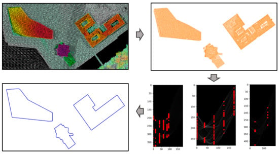
An overview of the proposed building outline extraction is illustrated in Figure 2.
3.1. Edge Point Selection
Our method requires ordered building edge points. Only the 2D coordinates of the edge points will be kept to extract building outlines. For this task, we apply the concave hull K-Nearest Neighbor algorithm [47] that uses the value of k as the only parameter to control the smoothness of the result. In the beginning, this algorithm finds its first vertex (point A) based on the lowest Y value. Then it will search k-nearest points (for k = 3: point B, C, D), as candidate for the next vertex. Point C will be assigned as the next vertex if it has the largest angle of right-hand turn measured from the horizontal line through point A. In the next step, the k nearest points of point C are queried, and the selected vertex is appointed once it has the largest angle of right-hand turn from line A–C. The process is repeated until the first vertex is selected once again as candidate.
Higher k will lead to smoother polygons. In this study, the k values vary from 3 to 11 depending on the point density. A building with irregular point intervals may require higher value of k to derive suitable edges.
3.2. Hough Accumulator Matrix
The key idea of the Hough transform is to select straight-line candidates based on a voting scheme in a parameter space. To parameterize a line, we use two parameters: distance to the origin, r, and orientation angle, . The mapping relations of a point in object space (x, y) and () parameter space is specified in Equation (1).
The chosen polar parameters are advantageous over the slope-intercept (m, c) parameterization since the (m, c) may have a singularity when the slope of the line is infinite. The number of rows and columns of the matrix is adjusted according to the bin sizes of the two parameters. Each cell contains a number of lines having and r values.
As illustrated in Figure 3a, one line defined by a pair may contain different building edge points, here A, B, and C. The fan of all lines passing through one point (Figure 3a) corresponds to a sinusoidal curve in Hough space (Figure 3b), while each point in Hough space corresponds to one straight line in object space.
For a given set of n ordered LiDAR points Pi = (xi, yi), for i = 1, 2, …n, forming a building roof boundary, a matrix R containing line distance r parameter values is created as follows:
- Fix origin O at (min xi, min yi) for (xi, yi), i = 1, 2, …, n and initiate a matrix R with dimension (n × 181);
- For point Pi and for each {0°, 1°, 2°,.., 180°}, determine ri() using Equation (1);
- Store ri in matrix R at position (i, ).
Matrix R stores r-values for lines of different angles (0° to 180°) through each point Pi. Next, it will be considered if points share lines. Lines common to many points are likely to define a building edge. To identify common lines, i.e., lines defined by different points but sharing the same values, the Hough Accumulator (HA) is created next. HA requires binning of r and θ to represent the location of its cells. Each cell in HA stores the number of points with matching θ and r. Different cells in HA represent different combinations of θ and r values. The higher the number in a HA cell, the more likely the cell produces a correct line for an edge.
HA is a 2D array of size (number of binr × 180). The trade-off between the number of bins of the matrix and the number of available observations is crucial [8]. Too many bins may lead to a sparse representation of the density that will decrease the ability to detect prominent lines. On the other hand, too few bins will reduce the resolution and accuracy of the building line results. We recommended that the bin width of r, (binr), is set according to the average point interval.
3.3. Detection of Arbitrary Building Directions
Building shapes and other man-made objects are often characterized by certain geometrical regularities [45], mostly appearing as perpendicularity or parallelism. However, in a reality, not every building is constructed using such geometrical regularities. Therefore, determining possibly arbitrary building direction is an important strategy for the building extraction process.
One limitation of Hough Transform is that when the number of lines increases, the correlated error around the peak in the parameter space could cause ambiguities for line [48]. To limit the search space for selecting line candidates, the proposed algorithm uses local maxima detection instead of global maxima. Local maxima are detected by identifying peaks in the graph of the variance of along the columns of the matrix HA. The variance is defined as the average of the squared deviations from the mean number of lines along the column of matrix HA. Finding local maxima means to detect accumulator cells that have higher vote than their neighborhood (peak). For detecting peaks, we first apply a Savitzky Golay filter [49] to denoise the data. The basic idea of Savitzky Golay filtering is to replace each point by the corresponding value of a least squares fit of a low order polynomial fitted to points in a window centered at that point.
In the smoothed variance data, peaks are detected if they meet two criteria: normalized threshold (amp) and minimum distance (mindist) between each detected peak. The normalized threshold will select peaks with higher amplitude than the threshold. Figure 4 illustrates the one-dimensional peak detection from a smoothed variance input (magenta graph) to define the direction. In most cases, the difference between two dominant building directions is close to 90°.
3.4. Hotspot Selection
After dominant directions are detected, the algorithm will next search along the corresponding columns for cells in matrix HA that have at least minL edge points. These cells are then preserved as initial hotspots. An initial hotspot is a candidate cell to represent a building line. The minimum edge length (minL) parameter is set based on the required building length, ℓ, as minL = , where d denotes the point interval. If, for example, the point interval is 0.5 m and the minimum length of the building edge to be extracted ℓ is 2.5 m, the required threshold minL = 5.
However, in HA, different column adjacent hotspots (one cell difference) may represent lines belonging to the same edge. This happens because some noise from the same edge points result in slightly different combinations. Hotspot filtering is applied by searching for any adjacent hotspots along a dominant direction. Only the hotspot that has maximal HA(i,j) value is kept. Figure 2d,e, respectively, present the result of initial hotspot detection and hotspot filtering.
3.5. Ordered Point List
One of our main contributions is to extract building outlines using a so-called Ordered Point List (OPL) matrix. This matrix is generated based on the classic Hough accumulator. OPL has the same dimension as HA and the same () parameters. The difference is that HA stores just the number of accumulated points voting for a line while OPL stores the actual ordered lists of points voting for a line. This means that each cell in OPL () contains an ordered list of points Pi that are on the parametric line r = .
To obtain more accurate and complete building edges, in OPL, the contents of each filtered hotspot is merged with its adjacent cells of the same column (Δbinr = 0 and Δbinr = 1). Matrix OPLm contains the merged point members. The difference cell value between HA, OPL, HAm, and OPLm of specific () is llustrated in Figure 5. Points accumulated in HA (Figure 5a) are specified in OPL (Figure 5b). The red cell marks one of the hotspots. Point members of hotspot cells of merged OPLm (a red cell in Figure 5d) are adapted by include neighboring cells. As an example, OPLm(105,87) has 11 additional points that complement the existing ordered point members of OPL(105,87).
3.6. Segment Detection and Filtering
Our algorithm yields arbitrary main directions that are used to select prominent lines. For some buildings with a complex shape, a false main direction may get detected because the corresponding θ has the highest vote in HA. Therefore, we apply hierarchical filtering to eliminate false lines resulting from a wrong main direction.
Using filtered hotspots and the merged Point Accumulator matrix OPLm as main input, the algorithm measures the distance of each point belonging to a filtered hotspot, to the hotspot line parameterized by the pair (). Then, it counts the number of hotspot points that have a distance more than binr. A hotspot will be removed from the list if one of two following conditions holds:
- It has at least 3 points having a distance more than binr;
- It has a mean distance d bigger than half binr value.
This mean distance threshold is set based on an empirical observation for detecting false lines and distinguishing those from correct but noisy lines.
A line resulting from the traditional Hough transform cannot distinguish different segments belonging to the same line. In this case, two different building edge segments that share the same () will not be detected. The proposed edge extraction algorithm requires segments, instead of lines, for producing a closed polygon. In this study, a segment is defined as a part of a line that is bounded by two building corner points. Note that a building line may contain more than one segment.
Segment detection exploits ordered edge points stored in OPLm. Each segment has a θ, an r, and a number of ordered points. Multiple segments on a line are identified by a gap or point jump between ordered points in the list. We set the gap threshold to 2 (two points jump). In this case, a gap is detected if there are at least two consecutive points missing from the list of ordered points.
An example of segment detection is illustrated in Figure 6. The red line in Figure 6a consists of two segments as a gap exists in the list of ordered points (L9) as presented in Figure 6b. Line L9 has two different segments. Point members of segment L9A are marked in red (from 58 to 77), while the point members of segment L9B are marked in blue (from 116 to 135). The two segments are separated by a large point interval.
A segment is then identified and selected as a list containing a minimum number of points minL. The minimum segment length is adjusted according to the output requirements. As an example, L1 in Figure 6b consists of two lists of ordered points separated by a big gap. Nevertheless, it will return one segment only because the first list of ordered points only has two members, points 0 and 1.
After all segments are identified, matrix OPLm contains different segments. These segments are sorted based on the first element of the list of points. Finally, segment filtering is performed. This last filtering step is needed to remove false segments that may remain in the result. A shorter segment having all points the same as a longer segment will be removed if one of two following conditions holds:
- The first point is not assigned as the last point of a longer segment;
- The last point is not assigned as first or last point of a longer segment.
Lists of points are input for corner extraction. First, all building segments are sorted based on their lowest participating point label. Then, the algorithm extracts intersections from consecutive segments. A closed building polygon is formed by connecting all consecutive segment intersections.
From two given parametric lines,
The intersection point c (xc, yc) is computed as
Table 1 summarizes different kind of point and line representations used in our proposed method. A point in object space is translated into a row in R, as a curve in HA, and as part of a list in OPL. Lines and segments in object space are represented by a subset of a column in R and as a cell in HA. A cell in HA shows the number of points belonging to the same line, while a cell in OPL shows the list of points of a line. Hence, in OPL, lines and segments are represented by list of several points.
3.7. Validation
Two different quantitative analyses are performed to evaluate the result of the building outline extraction: performance metrics and positional accuracy. The ground truth used as reference to assess our results is described in Section 4. We used three performance metrics [50] to evaluate the building polygon results, completeness (Cp), correctness (Cr), and quality (Q). The performance metrics are calculated based on an area comparison of buildings in the reference data and in the result in the unit m2.
The positional accuracy is a geometric validation that evaluates if the quality of the extracted building polygons meets the geometric accuracy criteria. The positional accuracy is determined using a Root Mean Square Error (RMSE) value. The squared root of the average of the squared differences between corner positions (X and Y coordinate) in the reference and in the result is calculated to estimate the RMSE.
where
- = Coordinates of resulting corner points
- = Coordinates of corner points in the ground truth
- n = Total number of corner points
4. Test Area and Preprocessing
4.1. Test Set Makassar
The test set is located in a newly built sub-urban area of Makassar city (Figure 7b), Sulawesi island of Indonesia. The LiDAR point density is between 8–10 points/m2 (ppm) and was acquired in 2012 using a Leica ALS70. The total study area is 1.2 km2 (Figure 7c). A topographic base map in vector format is used as ground truth (Figure 7a).
The LiDAR data we use has already been filtered into ground and non-ground points using TerraScan software. The software implements a Progressive TIN Densification, originating by Axelsson [51], to filter non-ground points. From the non-ground points, the building roof points are separated from the tree points using two thresholds: point distance to planar surface (0.2 m) and minimum segment size (30 m2).
The 3D building points as output by TerraScan are then segmented into different clusters using the DBSCAN algorithm. DBSCAN segmentation [52] requires two parameters: radius distance (eps) and minimum number of points (minPts). To find a segment, DBSCAN starts with an arbitrary seed point p and then retrieves all neighboring points (density-reachable) from p that are located within a given eps and contains a given minPts. Outliers are defined once minPts cannot be achieved within the given eps. The cluster will grow as long as nearby points within the eps distance from seed p fulfill the minPts threshold. In case minPts within distance eps is not fulfilled, a point or group of points is considered as outlying. During the cluster growing, outliers may change into a member of one of the clusters once they are within the eps distance from the active seed point. To grow the next cluster, a next seed that does not belong to any cluster is chosen. The clustering stops once all points are assigned.
The parameter thresholds used for the Makassar dataset are eps = 1.2m and minPts = 3. This means that the required minimum number of points assigned as a cluster within 1.2 m from the seed points is three points. The segmented 3D building points resulting from DBSCAN after size filtering are shown in Figure 7d.
4.2. Test Set Vaihingen
The second area of study belongs to the Vaihingen test set provided by the ISPRS (International Society for Photogrammetry and Remote Sensing). The LiDAR point density varies between 4–7 points/m2 (ppm). This data was acquired in August 2008 by a Leica ALS50 airborne LiDAR system. There are two sub areas, Vaihingen-A and Vaihingen-B, as presented in Figure 8. The Vaihingen-A dataset consists of residential buildings of complex shape surrounded by trees. Ground truth for Vaihingen-A comprises a set of building references from OpenStreetMap (OSM), confirmed by true orthophotos provided by the ISPRS. The Vaihingen-B test set, which is basically the same dataset as Vaihingen Area 2 as described on the ISPRS webpage [53], is characterized by complex high-rise buildings that have several roof layers at different height. This benchmark dataset is chosen and used by several similar studies [25,28,32,33] to test and compare their algorithms. For Vaihingen-B, we use 2D building outlines in vector format as provided by ISPRS [54] as ground truth.
For the Vaihingen-A test set, we use the surface growing function of Point Cloud Mapper (PCM) developed by Vosselman [55] to perform point cloud segmentation. Surface growing thresholds implemented in this study are as follows:
- Seed surface selection. At least 10 points out of 20 nearest points within a 1-m radius are used to check for neighborhood planarity and apply a 3D Hough transform. Seeds are extended to other points located within a 1-m radius with a height difference of less than 20 cm to the fitted plane. The bin sizes of the distances and angles of the 3D Hough transform are set to 20 cm and 3 degrees;
- Growing expansion. Once a seed segment is found, region growing looks for adjacent points belonging to the same plane. Points are assigned to a plane if the distance to the corresponding plane is 50 cm maximum.
A different segmentation method is applied for Vaihingen-B. First, the point cloud is classified using the LAStools software developed by Rapidlasso [56]. We then preserved only the planar points using plane detection to remove remaining tree points. The planar points are then segmented using DBSCAN (eps = 1.2m and minPts = 3). The test set of the Vaihingen-A and the Vaihingen-B, as well as the segmentation and classification results, are presented in Figure 9.
4.3. Test Set Amsterdam
An additional point cloud dataset sampling the EYE-Amsterdam neighborhood (Figure 10a) demonstrates the ability of our algorithm to extract complex buildings of multiple arbitrary directions. We use an open source AHN3 point cloud dataset downloaded from PDOK [57]. Point clouds of AHN3 acquired in 2014 are already classified into several classes (ground, building, water, etc.). The AHN3 classified building points of our EYE-Amsterdam study area is shown in Figure 10d.
5. Sensitivity Analysis and Experiments
This section describes common issues that highlight specific features of our algorithm to answer the research objectives. The last paragraph presents a sensitivity analysis of the parameters used.
5.1. Detecting Multiple Arbitrary Direction
The EYE building (as indicated by a white star in Figure 10d) has a unique shape, which makes it impossible to apply perpendicularity rules. The A’DAM Lookout building (as indicated by a green star in Figure 10d) is another complex building in this area with five building directions of different edge length. The ability of our proposed algorithm for extracting outlines of such complex building shapes is illustrated in Figure 11. Based on the detection of multiple arbitrary building directions (Figure 11a), the building segments are identified (Figure 11b). As the final output, based on corners of consecutive building segments, a closed building polygon is formed (Figure 11c).
Herout [12] stated that the accuracy of the Hough Transform is strongly dependent on the detection of maxima in parameter space. As local maxima for detecting arbitrary building directions depend on the number of votes, it is possible that edge points of a complex building dominantly vote for an incorrect building direction. This situation may cause the algorithm to detect false building lines that are supported by many edge points but are not part of any building segment.
Figure 12 illustrates the detection of a false dominant direction resulting in a false building line. The false main direction is likely caused by a special building geometry shape that allows most of the edge points from two different directions to vote for the same direction. In this case, parallel short building edges result in false lines. However, by adding a filtering step to our workflow, the algorithm is able to eliminate and remove these false lines. In Figure 12a, initial hotspots are detected based on three dominant directions at = 7°, = 78°, and = 96°. The yellow line, at = 78°, marks the falsely detected dominant direction corresponding to the false green lines in Figure 1b. All lines corresponding to initial hotspots are shown in Figure 12b, where false lines are shown in green and correct lines in red. Figure 12c shows the results of our proposed segment filtering procedure.
5.2. Extraction of Different Interrupted Segments of Different Length
One drawback of traditional Hough Transform is its difficulty to distinguish different segments that are collinear as any segment with the same () parameters will be considered as the same line [58]. Moreover, in the application of traditional Hough transform, short segments only result in low peaks, which makes them difficult to identify [13,59]. Because of this limitation, it is a problem to identify short building edges especially if long edges exist of different direction. Figure 13a,b, respectively, show that building outlines of different length and building outlines of collinear line segments (as indicated by red ellipses) are correctly extracted using the proposed method. By exploiting gaps in the ordered edge points of each line, segments that are collinear can be detected and separated.
5.3. Robustness to Noise and Irregularity
In general, our method has the ability to create correct outlines of noisy edge points and straighten up such imperfect building edges. Adjacent trees may cause flaws or irregularities in building segmentation results. This situation, later on, may induce an incorrect building outline. Our proposed method eliminates and removes the influence of such building irregularity. Figure 14a,c, respectively, show the outline results in case of over-segmentation for a rectangular and complex building shape by using the proposed method. Both buildings have flaws due to connected trees. In such cases, the algorithm has two possibilities to produce a correct building outline. First, due to sparse and irregular distribution of tree points, the number of edge points of the tree is less than the minimum length edge (minL) threshold. Second, in case the number of edge tree points is more than minL, the extracted line segments of the tree edges do not form a fully closed polygon. As the proposed algorithm uses consecutive lines based on ordered points to extract the corresponding corners, extraction of false corners is avoided.
The capability of our algorithm to deal with irregularities may extend to an incomplete building roof case (under-segmentation). Figure 14b shows the outline of a building roof that is partially covered by an adjacent tree. Correct lines are still obtained although there is a gap consisting of missing edge points in the middle building edge part.
5.4. Sensitivity Analysis
We have implemented a data-driven method that may require parameter tuning for areas of different characteristics. Parameters need to be set for using the proposed procedure are discussed as follows:
- Bin size: to determine cell size and distribute the edge points in a specific row (binr) and column (binθ). We fix binθ at (1 degree), while the size of the binr is variable, depending on the point density. For the Makassar and the Vaihingen datasets, binr varies between 0.3 to 0.6 m.
- Local maxima: to detect dominant building directions. Two parameters to determine dominant directions are the amplitude (amp) and the minimum distance (mindist) between each detected local maximum. The recommended threshold for amp is 0.5 m and mindist is 30°. In case of complex building shapes and noisy data, an amp threshold between 0.15–0.2 m and a mindist value between 15°–30° is recommended.
- Minimum number of points: to determine initial hotpots. The minL value is determined based on the length of the building edge that is required to be extracted. We applied a smaller edge threshold for the Vaihingen test set as this dataset has complex buildings with many short edges (±1.5 m). The edge threshold for Vaihingen is set to 3 points. For AOI-1 Makassar, minL is set to five points. This threshold is set as the minimum length of a building segment length that needs to be extracted is 2.5 m.
Recap of parameter setting used in this study is presented in Table 2.
Each Hough Accumulator matrix HA cell contains the number of edge points that vote for the same () value. Bin size determination is a crucial step that influences the point distribution of edge points into each cell in HA. If the bin size is set too big, it may result in the coinciding of different edges or less accurate line results. On the other hand, if we set the bin size too small, some particular building edges may not be identified. The bin size for θ (binθ) is set to 1°. Experiments show that the determined binθ is sufficient to find line candidate. For point clouds with a point interval between 0.3 and 0.7 m, we set the binr size to 0.5 m.
We conducted an additional experiment to identify a sufficient binr value as well as to evaluate the sensitivity of the binr parameter. Two different building shapes (simple and complex) with a point interval from 0.4 to 0.7 m are used for this experiment. As simple building case, a building with a rectangular roof with 4 lines/corners is used. As complex case, we select a building with 24 lines/corners. The results of the experiment are presented in Table 3.
For the experiment, all required parameters have the same value except binr. The results indicate that the smaller the bin size, the smaller the average of standard deviation and the RMSE. However, at the same time, the possibility to produce additional segments or corners that are not always correct increases. We also present the total number of edge points that is not used by any line to notify any incomplete or suspicious line result. In Table 3, a simple (square shape) building with binr = 30 cm and binr = 20 cm yields three dominant directions that could result in false lines. However, for binr = 30 cm, our method is able to eliminate these false lines by obtaining four building line segments with acceptable RMSE. Meanwhile, for binr = 20 cm, our method fails to deliver a complete building outline, as five points remain unused.
The sensitivity of binr is increasing for a complex building. As this building has many line segments with significant length difference between the short and long segments (short edges have 3–4 points, while longer edges have 12–20 points), the determination of binr affects the line segments results (number of extracted segments and RMSE). Moreover, the small distance between several parallel building edges yields false dominant directions. In Table 3 a binr size that is smaller or bigger than the point interval (which is between 40 and 70 cm) results in an incomplete building outline, which is indicated by the presence of remaining points or no RMSE result (N/A).
The distribution of resulted segment intersections for different bin sizes (from binr = 40 cm to binr = 80 cm) is illustrated in Figure 15a. Different intersections of different bin sizes are indicated by different colors. Grey circles indicate a 1-m buffer of reference building corner. Some intersections located in the middle of building edge (as indicated by the blue circle in Figure 15b) are obtained using binr = 70 cm and binr = 80 cm. However, these corners do not affect the shape of the polygon, as they are collinearly located between two other corners.
The proposed building outline extraction works for single buildings. It requires a pre-processing step to select and acquire the outer building edge points. In certain cases, the proposed algorithm may fail to extract building outlines correctly due to heavy noise and errors in the segmentation. In this case, parameter tuning (binr and/or local maxima) may solve the problem, as the binning process of such irregular edge points may result in bad point division, and a voting scheme that makes the algorithm fail to detect correct local maxima.
Considering the aforementioned problems, a scheme for quality checking of the output is necessary to increase the applicability of our method for map production. We define a strategy to assist the quality checker in case of an incorrect or doubtful result. A missing line or a shifted line that causes incomplete or incorrect building polygons can be detected from the number of edge points that is not used by any extracted line. Based on this, the human operator may decide to perform a manual check and confirm the result. This procedure is expected to accelerate quality control and minimize manual editing.
6. Results and Discussion
In the following, we will discuss the overall results of the proposed method. A more detailed discussion of the experiments for the Makassar test set and the Vaihingen test sets respectively, are given next. Finally, a comparison to previous results on the benchmark test set (Vaihingen-B) is presented.
6.1. General Evaluation
Goal of this study is to provide a robust procedure for automatic building outline extraction from airborne LiDAR point clouds. Using the ground truth described in Section 4, we evaluate our method. Our method is able to achieve high completeness and correctness for both study areas as shown in Table 4. For Makassar, building polygons results achieve 91.8% completeness, 99.2% correctness and 91.1% quality. The quality metrics of the Vaihingen-A test set are also high, 96.4%, 96.5%, and 93.2%, respectively. Vaihingen-B achieves slightly less good quality metrics of 90.1% completeness, 99.4% correctness and 89.6% quality.
We use different methods of point cloud filtering, classification, and segmentation to assure that our building extraction method is able to adapt to and is not limited to a specific processing workflow. The proposed workflow for extracting building outlines requires segmentation as a pre-processing step. The quality of the segmentation result influences the extracted building outlines. Irregular concave hull outlines as shown in Figure 2b, are not suitable as input for map products. Table 2 shows a comparison between an object-based evaluation of our results and the concave hull of the segmented building points. Our results have better quality and correctness, with an increase of between 1% and 3%, except for Vaihingen-B. This proves that our algorithm is able to increase the quality of building outlines resulting from the concave hull and improve the segmentation result quality.
It should also be noted that the computational performance of the proposed method is not an issue. The average computation time of the proposed OHT method for delineating 2D building outlines on an Intel Core 2Duo CPU with a 2.4 GHz processor is about 0.579s per-building.
The completeness of our building outlines results is lower than the correctness. This means that, on average, building polygons are smaller than the ground truth data. As LiDAR points rarely sample a building edge, only points located within the building roof are used, which causes a shrinking of the polygons. We estimated the percentage of shrinking area using all buildings of simple (square) size that are well-segmented in our test sets. The average of the building shrinking is consistent at 4.24% for the Makassar test set and 4.36% for the Vaihingen test sets.
6.2. Results for Makassar
Indonesian base map specifications [46] require that each building edge of at least 2.5 m should be presented on the map. Accordingly, the minimum length minL of a segment for the Makassar test set is five points (2.5m/0.5m). The binr size is set to 0.5 m. The ground truth data used as reference for Makassar is the Indonesian base map at a scale of 1:10,000. The base map is obtained by manual 3D-compilation of stereo-photos acquired at the same time and from the same platform as the LiDAR data we use.
The comparison between the extracted building polygons of Makassar and the ground truth is presented in Figure 16b. From 42 buildings present on the base map, 37 buildings are extracted. The five missing buildings are indicated by blue stars. In addition, our method is able to extract one building that is not present in the ground truth (as indicated by a black arrow in Figure 16b). This building has a size of 15.5 m by 43 m and should have been present in the base map.
Even though some noise exists in the segmented building points, the proposed method is still able to extract accurate building polygons. As highlighted in Figure 16a, most filtered building segments (showed in blue) are noisy. High vegetation points connecting to the buildings cause most of the noise. Six buildings have a size or shape different from the base map (indicated by black stars) due to imperfect filtering and segmentation of building points. Low elevation of building roof points is assumed as the main cause why five buildings (indicated by blue arrows) are completely missing.
Positional accuracy is measured for buildings that exist in our result and the base map. RMSE is measured based on the coordinate differences between building corners from our result and reference data. The RMSE for complete building polygons is between 0.38–0.57 m. For a building where some parts of its roof are not completely detected (as indicated by the black circle in Figure 16b), the building corners shift reaches 10.84 m.
During the experiment, the proposed method can actually extract building edges of a length less than the required 2.5 m from the Makassar data. The two buildings, as indicated by red arrows in Figure 16b, are annexes of a size of 1.3 m by 6 m. These building annexes are likely not included in the map, as their size does not meet the 1:10,000 base map specification. Our method is able to extract such small building parts by applying the minimum edge length paramater minL to minL = 3.
6.3. Results for Vaihingen
The chosen test sets of Vaihingen consist of high-residential buildings that have complex shape and are surrounded by trees. Several buildings have multiple roof layers of different heights and various length of edges. We set 1.5 m as the minimum length of a building line segment corresponding to minL = 3 for both of the Vaihingen test sets. The binr size setting is between 0.3 and 0.6 m.
We succeeded to extract all buildings in the Vaihingen-A and the Vaihingen-B test set. For the Vaihingen-A test set, the reference data is acquired by Open Street Map (OSM) validated by aerial orthophotos provided by ISPRS. For the Vaihingen-B test set, we use a set of building outlines provided by ISPRS as the ground truth. The RMSE result of buildings in the Vaihingen-A data that are completely segmented is between 0.2–0.37 m. As shown in Figure 17b, five out of 27 buildings have different shape due to over-segmentation (three red stars) or under-segmentation (three black stars) due to dense trees above the building roof.
The RMSE of extracted building corners is between 0.19–0.96 m. According to the ground truth, the Vaihingen-B results have the lowest quality metrics among our three test sets. The main cause for a lower quality metric is mis-detection of a vegetated building roof part of significant size (8.5 m by 9.5 m), marked by the black circle in Figure 17c, which is likely a low roof covering an underground basement. The filtering process failed to detect this roof part as a building as the height difference between this basement roof and the ground is less than 1 m. The Digital Surface Model (DSM) of this subset area, as presented in Figure 18b, shows that height information may not help to detect this kind of building (inside the white circle). In addition, some vegetated building roofs are not completely detected (indicated by brown circles in Figure 18a,b). This happens because the trees and their surroundings disturb the expected planarity.
In the results, several building polygons have a shape and size different from the ground truth because of tree points allocated to the segmented building points. High vegetation adjacent to buildings is the main cause for the high false positive rate of the building polygon results. Moreover, neighboring trees that cover some parts of the roof induce some false negatives. For example, in Figure 19a, the building segment contains parts of four adjacent trees. These tree points have similar height as the building roof, which range from 275.5 to 276.5 m. The height difference to the mean is about 40 cm as shown in Figure 19c. However, our line extraction algorithm is able to ignore 1 out of 4 trees as indicated by the yellow circle in Figure 19a. An extra feature, such as intensity as shown in Figure 19d may not work for obtaining a correct outline for this building case. A trade off in using the intensity value to remove trees will reduce the building completeness as there is a roof part covered by a big tree. An additional clustering step (using e.g., DBSCAN) may work to remove trees. Nevertheless, when a building roof is covered by dense trees (e.g., as marked by the purple circle in Figure 19a), orthogonal input data (such as ALS point cloud data or airborne images) may not work to detect the building boundaries accurately.
6.4. Comparison to Previous Building Outline Works
An analysis is performed to compare the performance of the proposed method to previous methods. Several previous results are selected from the Vaihingen-B evaluation, which is available on the ISPRS web page (http://www2.isprs.org/commissions/comm3/wg4/results/a2_detect.html) and confirmed by the corresponding articles. We only consider methods aiming at obtaining straight building outlines that implement a data-driven approach and apply a regularization approach similar to our research objective. The selection is also limited to works that use ALS point clouds or a combination of ALS point clouds and aerial photos as input. We also include two results that are not presented on the ISPRS web page [25,33] in our comparison.
As shown in Table 5, the MON3 represents Siddiqui et al. [28] method has highest completeness but this method uses additional color information from aerial photos to get straight lines. Building boundaries in the Vaihingen-B test set are clearly recognizable as bold white pixels in the aerial photos. Hence, the low building roof (as marked by the white circle in Figure 18a) as well as vegetated roofs (as marked by the brown circle in Figure 18a) can still be detected. However, the lower correctness metric of the MON3 method indicates that some buildings may be over-segmented. On the contrary, our method has best correctness and quality metric for this test set. The higher quality metric indicates that our method delivers complete and accurate building polygon results.
Our proposed method requires building roof points as input. Then, the 2D edge points are transformed to Hough space to obtain prominent building outlines. Based on this scheme, as long as building points are given, our method should work for arbitrary point cloud data including point clouds generated from images by for example dense image matching process.
7. Conclusions and Future Work
We have presented a framework for delineating 2D building outlines automatically from segmented ALS point clouds. An adaptive approach to obtain boundary lines of different building shapes and sizes is developed based on an extension of Hough transformation exploiting the order of points forming a building outline. Point votes for all possible lines passing through given edge points are stored in a Hough accumulator matrix. Based on the accumulator matrix, the algorithm uses local maxima for detecting dominant building orientations. The prominent lines are selected based on detected dominant directions. A hierarchical filtering approach by empowering the Hough transform with ordered edge points is introduced to select correct building segments and derive accurate building corners. Many problems that occur with the original Hough Transform are avoided.
Our enhanced Hough transformation method, which exploits the ordered points and regularity, gives a substantial improvement in the quality of building outline extraction as concluded from a comparison to existing benchmark results. Based on our extensive evaluation, the proposed procedure is able to deliver high completeness and correctness as well as high positional accuracy. Even though the Hough transformation involves many matrices, aside from the pre-processing step, the processing speed to process the building outline is not an issue as the proposed algorithm works per single building. Another advantage of the proposed method is that it directly uses the point cloud. No data conversion or additional data is required. The proposed procedure is tested on different areas to verify the robustness of our method to the variation of different data specifications, and urban landscape characteristics. In case noise and small flaws exist in the data, the voting scheme of the Hough transform makes our method feasible for preserving the actual building shape and size. Implementation of the proposed outline extraction on different building segmentation attests that the use of the algorithm is not limited to a particular segmentation method.
We implemented a data-driven method that involves directed regularization that works effectively to detect multiple building orientations and derive accurate straight outlines. Our algorithm, accordingly, has limitation to detect curved outlines. As the algorithm requires edge points for delineating outlines, it is sensitive to the pre-processing steps, which are segmentation and concave hull. It may require parameter tuning for different dataset and different output requirements to achieve satisfactory results. Therefore, to guarantee an optimal result, understanding the input data and determining output criteria is necessary.
Extension of the present work should consider the implementation and performance evaluation of the proposed method for massive map production. Applying a robust classification and segmentation method for a larger area may become one of the challenges in future, as it may influence the outline extraction result. Application of Hough transform for curved buildings should also be elaborated.
Author Contributions
E.W. designed the workflow and conducted the experiments described in the paper, and responsible for the main structure and writing of the paper. R.L. gave comments and editions to paper writing, B.G. provided comments for the paper.
Funding
This research was financially supported by the Indonesia Endowment Fund for Education (LPDP) as a part of PhD research conducted under the Department of Geoscience and Remote Sensing of TU Delft and the APC was funded by Delft University of Technology.
Acknowledgments
The authors acknowledge Indonesian Geospatial Agency (www.big.go.id) for providing the Makassar dataset in this research.
Conflicts of Interest
The authors declare no conflict of interest.
References
- Rottensteiner, F.; Briese, C. A new method for building extraction in urban areas from high-resolution LIDAR data. Int. Arch. Photogramm. Remote Sens. Spat. Inf. Sci. 2002, 34, 295–301. [Google Scholar]
- Sohn, G.; Dowman, I. Data fusion of high-resolution satellite imagery and LiDAR data for automatic building extraction. ISPRS J. Photogramm. Remote Sens. 2007, 62, 43–63. [Google Scholar] [CrossRef]
- Widyaningrum, E.; Gorte, B.G.H. Comprehensive comparison of two image-based point clouds from aerial photos with airborne LiDAR for large-scale mapping. Int. Arch. Photogramm. Remote Sens. Spat. Inf. Sci. 2017, 42. [Google Scholar] [CrossRef]
- Gamba, P.; Dell’Acqua, F.; Lisini, G. BREC: The Built-up area RECognition tool. In Proceedings of the 2009 IEEE Joint Urban Remote Sensing Event, Shanghai, China, 20–22 May 2009; pp. 1–5. [Google Scholar]
- TerraScan. Available online: http://www.terrasolid.com/products/terrascanpage.php (accessed on 3 July 2019).
- ENVI. Available online: https://www.harrisgeospatial.com/Software-Technology/ENVI (accessed on 3 July 2019).
- Golubiewski, N.; Lawrence, G.; Fredrickson, C. Constructing Auckland: 2013 Building Outlines Update in the Urban Core and Its Periphery; Auckland Technical Report TR2019/006; Auckland Council: Auckland, New Zealand, 2019.
- Susetyo, D.B.; Hidayat, F.; Hariyno, M.I. Automatic building model extraction using LiDAR data. In Proceedings of the Asian Conference and Remote Sensing, Kuala Lumpur, Malaysia, 15–19 October 2018. [Google Scholar]
- Princen, J.; Illingworth, J.; Kittler, J. A formal definition of the Hough transform: Properties and relationships. J. Math. Imag. Vis. 1992, 1, 153–168. [Google Scholar] [CrossRef]
- Duda, R.O.; Hart, P.E. Use of the Hough transform to detect lines and curves in pictures. Commun. ACM 1972, 15, 11–15. [Google Scholar] [CrossRef]
- Vozikis, G.; Jansa, J. Advantages and disadvantages of the Hough transformation in the frame of automated building extraction. In Proceedings of the XXI ISPRS Congress, Beijing, China, 3–11 July 2008; Volume 37, pp. 719–724. [Google Scholar]
- Herout, A.; Dubská, M.; Havel, J. Variants of the Hough transform for straight line detection. In Real-Time Detection of Lines and Grids; Springer: London, UK, 2013; pp. 17–34. [Google Scholar]
- Lee, J.W.; Kweon, I.S. Extraction of line features in a noisy image. Pattern Recognit. 1997, 30, 1651–1660. [Google Scholar] [CrossRef]
- Bertasius, G.; Shi, J.; Torresani, L. High-for-low and low-for-high: Efficient boundary detection from deep object features and its applications to high-level vision. In Proceedings of the IEEE International Conference on Computer Vision, Santiago, Chile, 11–18 December 2015; pp. 504–512. [Google Scholar]
- Shen, W.; Wang, X.; Wang, Y.; Bai, X.; Zhang, Z. Deepcontour: A deep convolutional feature learned by positive-sharing loss for contour detection. In Proceedings of the IEEE Conference on Computer Vision and Pattern Recognition, Boston, MA, USA, 7–12 June 2015; pp. 3982–3991. [Google Scholar]
- Liu, Y.; Cheng, M.; Hu, X.; Bian, J.; Zhang, L.; Bai, X.; Tang, J. Richer convolutional features for edge detection. IEEE Trans. Pattern Anal. Mach. Intell. 2017, 41, 1939–1946. [Google Scholar] [CrossRef] [PubMed]
- Yang, J.; Price, B.; Cohen, S.; Lee, H.; Yang, M. Object contour detection with a fully convolutional encoder-decoder network. In Proceedings of the IEEE Conference on Computer Vision and Pattern Recognition (CVPR), Las Vegas, NV, USA, 27–30 July 2016; pp. 193–202. [Google Scholar]
- Wang, Y.; Zhao, X.; Li, Y.; Huang, K. Deep crisp boundaries: From boundaries to higher-level tasks. IEEE Trans. Image Process. 2019, 28, 1285–1298. [Google Scholar] [CrossRef]
- Kelm, A.P.; Rao, V.S.; Zolzer, U. Object Contour and Edge Detection with RefineContourNet. arXiv 2019, arXiv:1904.13353. [Google Scholar]
- Lu, T.; Ming, D.; Lin, X.; Hong, Z.; Bai, X.; Fang, J. Detecting building edges from high spatial resolution remote sensing imagery using richer convolution features network. Remote Sens. 2018, 10, 1496. [Google Scholar] [CrossRef]
- Deng, R.; Shen, C.; Liu, S.; Wang, H.; Liu, X. Learning to predict Crisp Boundaries. In Proceedings of the European Conference on Computer Vision (ECCV), Munich, Germany, 8–14 September 2018; pp. 562–578. [Google Scholar]
- Microsoft GitHub Repository. Available online: https://github.com/Microsoft/USBuildingFootprints (accessed on 19 May 2019).
- Yu, L.; Li, X.; Fu, C.W.; Cohen-Or, D.; Heng, P.A. EC-Net: An Edge-aware Point set Consolidation Network. In Proceedings of the European Conference on Computer Vision (ECCV), Munich, Germany, 8–14 September 2018; pp. 386–402. [Google Scholar]
- Li, Y.; Wu, H.; An, R.; Xu, H.; He, Q.; Xu, J. An improved building boundary extraction algorithm based on fusion of optical imagery and LIDAR data. Optik 2013, 124, 5357–5362. [Google Scholar] [CrossRef]
- Zhao, Z.; Duan, Y.; Zhang, Y.; Cao, R. Extracting buildings from and regularizing boundaries in airborne LiDAR data using connected operators. Int. J. Remote Sens. 2016, 37, 889–912. [Google Scholar] [CrossRef]
- Awrangjeb, M. Using point cloud data to identify, trace, and regularize the outlines of buildings. Int. J. Remote Sens. 2016, 37, 551–579. [Google Scholar] [CrossRef]
- Akbulut, Z.; Özdemir, S.; Acar, H.; Karsli, F. Automatic Building Extraction from Image and LiDAR Data with Active Contour Segmentation. J. Indian Soc. Remote Sens. 2018, 46, 2057–2068. [Google Scholar] [CrossRef]
- Siddiqui, F.U.; Teng, S.W.; Awrangjeb, M.; Lu, G. A robust gradient based method for building extraction from LiDAR and photogrammetric imagery. Sensors 2016, 16, 1110. [Google Scholar] [CrossRef]
- Xie, L.; Zhu, Q.; Hu, H.; Wu, B.; Li, Y.; Zhang, Y.; Zhong, R. Hierarchical Regularization of Building Boundaries in Noisy Aerial Laser Scanning and Photogrammetric Point Clouds. Remote Sens. 2018, 10, 1996. [Google Scholar] [CrossRef]
- Awrangjeb, M.; Lu, G.; Fraser, C. Automatic building extraction from LiDAR data covering complex urban scenes. Int. Arch. Photogramm. Remote Sens. Spat. Inf. Sci. 2014, 40, 25. [Google Scholar] [CrossRef]
- Dorninger, P.; Pfeifer, N. A comprehensive automated 3D approach for building extraction, reconstruction, and regularization from airborne laser scanning point clouds. Sensors 2008, 8, 7323–7343. [Google Scholar] [CrossRef] [PubMed]
- Gilani, S.A.N.; Awrangjeb, M.; Lu, G. An automatic building extraction and regularisation technique using LiDAR point cloud data and orthoimage. Remote Sens. 2016, 8, 258. [Google Scholar] [CrossRef]
- Huang, R.; Yang, B.; Liang, F.; Dai, W.; Li, J.; Tian, M.; Xu, W. A top-down strategy for buildings extraction from complex urban scenes using airborne LiDAR point clouds. Infrared Phys. Technol. 2018, 92, 203–218. [Google Scholar] [CrossRef]
- Sampath, A.; Shan, J. Building boundary tracing and regularization from airborne LiDAR point clouds. Photogramm. Eng. Remote Sens. 2007, 73, 805–812. [Google Scholar] [CrossRef]
- Lach, S.R.; Kerekes, J.P. Robust extraction of exterior building boundaries from topographic LiDAR data. IEEE Int. Geosci. Remote Sens. Symp. 2008, 2, 85–88. [Google Scholar] [CrossRef]
- Illingworth, J.; Kittler, J. A survey of the Hough transform. Comput. Vis. Graph. Image Process. 1988, 44, 87–116. [Google Scholar] [CrossRef]
- Mukhopadhyay, P.; Chaudhuri, B.B. A survey of Hough Transform. Pattern Recognit. 2015, 48, 993–1010. [Google Scholar] [CrossRef]
- Herout, A.; Dubská, M.; Havel, J. Review of Hough Transform for Line Detection. In Real-Time Detection of Lines and Grids; Springer: London, UK, 2013; pp. 3–16. [Google Scholar] [CrossRef]
- Morgan, M.; Habib, A. Interpolation of LiDAR data and automatic building extraction. In Proceedings of the ACSM-ASPRS Annual Conference, Washington, DC, USA, 19–26 April 2002; pp. 432–441. [Google Scholar]
- Guercke, R.; Sester, M. Building footprint simplification based on Hough transform and least squares adjustment. In Proceedings of the 14th Workshop of the ICA commission on Generalisation and Multiple Representation, Paris, France, 30 June–1 July 2011. [Google Scholar]
- Dalitz, C.; Schramke, T.; Jeltsch, M. Iterative Hough transform for line detection in 3D point clouds. Image Process. Line 2017, 7, 184–196. [Google Scholar] [CrossRef]
- Miller, J. Building Extraction from LiDAR Using Edge Detection. Ph.D. Thesis, Department of Geoinformatics and Geospatial Intelligence, Shenandoah University, Winchester, VA, USA, 2016. [Google Scholar]
- Oesau, S. Geometric Modeling of Indoor Scenes from Acquired Point Data. Ph.D. Thesis, Université Nice Sophia Antipolis, Nice, France, 2015. [Google Scholar]
- Albers, B.; Kada, M.; Wichmann, A. Automatic extraction and regularization of building outlines from airborne LiDAR point clouds. Int. Arch. Photogramm. Remote Sens. Spat. Inf. Sci. 2016, 41. [Google Scholar] [CrossRef]
- Hohle, J. Generating topographic map data from classification results. Remote Sens. 2017, 9, 224. [Google Scholar] [CrossRef]
- SNI 8205:2015. Indonesian National Standard for Base Map Accuracy (Ketelitian Peta Dasar). Available online: http://sispk.bsn.go.id/SNI (accessed on 25 August 2018).
- Moreira, A.; Santos, M.Y. Concave hull: A k-nearest neighbours approach for the computation of the region occupied by a set of points. In Proceedings of the GRAPP International Conference on Computer Graphics Theory and Applications, Barcelona, Spain, 8–11 March 2007. [Google Scholar]
- Leavers, V.F. The dynamic generalized Hough transform: Its relationship to the probabilistic Hough transform and an application to the concurrent detection of circles and ellipses. CVGIP Image Underst. 1992, 56, 381–398. [Google Scholar] [CrossRef]
- Savitzky, A.; Golay, M.J. Smoothing and differentiation of data by simplified least squares procedures. Anal. Chem. 1964, 36, 1627–1639. [Google Scholar] [CrossRef]
- Rutzinger, M.; Rottensteiner, F.; Pfeifer, N. A comparison of evaluation techniques for building extraction from airborne laser scanning. IEEE J. Sel. Top. Appl. Earth Observ. Remote Sens. 2009, 2, 11–20. [Google Scholar] [CrossRef]
- Axelsson, P.E. DEM generation from laser scanner data using adaptive TIN models. Int. Arch. Photogramm. Remote Sens. 2000, 32, 110–117. [Google Scholar]
- Ester, M.; Kriegel, H.P.; Sander, J.; Xu, X. A density-based algorithm for discovering clusters in large spatial databases with noise. In Proceedings of the 2nd International Conference on Knowledge Discovery and Data Mining (KDD-96), Portland, OR, USA, 2–4 August 1996. [Google Scholar]
- ISPRS Test Project on Urban Classification and 3D Building Reconstruction. Available online: http://www2.isprs.org/tl_files/isprs/wg34/docs/ComplexScenes_revision_v4.pdf (accessed on 24 August 2018).
- ISPRS. Vaihingen Results: Urban Object Detection in Area 2. Available online: http://www2.isprs.org/commissions/comm3/wg4/results/a2_detect.html (accessed on 11 December 2018).
- Vosselman, G.; Gorte, B.G.H.; Sithole, G.; Rabbani, T. Recognising structure in laser scanner point clouds. In ISPRS 2004: Proceedings of the ISPRS Working Group VIII/2: Laser Scanning for Forest and Landscape Assessment; Thies, M., Koch, B., Spiecker, H., Weinacher, H., Eds.; University of Freiburg: Freiburg, Germany, 2004; pp. 33–38. [Google Scholar]
- LAStools. “Efficient LiDAR Processing Software” (Version 141017, Academic). Available online: http://rapidlasso.com/LAStools (accessed on 6 October 2018).
- Kadaster and Geonovum. Publieke Dienstverlening Op de Kaart (PDOK). Available online: https://www.pdok.nl/ (accessed on 24 August 2018).
- Zhang, Y.; Webber, R. A windowing approach to detecting line segments using Hough transform. Pattern Recognit. 1996, 29, 255–265. [Google Scholar] [CrossRef]
- Guerreiro, R.F.; Aguiar, P.M. Connectivity-enforcing Hough transform for the robust extraction of line segments. IEEE Trans. Image Process. 2012, 21, 4819–4829. [Google Scholar] [CrossRef] [PubMed]
Figure 1.
The general procedure for extracting high quality straight building outlines.

Figure 2.
The proposed Ordered point aided Hough Transform (OHT) workflow for building outline extraction. (a) Building points; (b) concave hull of a building roof; (c) detection of dominant directions using local maxima; (d) detection of initial hotspots along dominant directions yields14 initial hotspots; (e) reduction to 10 filtered hotpots; (f) 10 lines corresponding to filtered hotspots; (g) Point accumulator analysis yields 12 segments; (h) segment intersection identifies 12 corners.

Figure 3.
Hough transform using (θ, r) parameters for detecting lines. (a) In object space, a line represented by an angle-distance (θ, r) passing through three points A, B, and C; (b) In Hough space, this line appears as the point of intersection of the curves , , and .
Figure 3.
Hough transform using (θ, r) parameters for detecting lines. (a) In object space, a line represented by an angle-distance (θ, r) passing through three points A, B, and C; (b) In Hough space, this line appears as the point of intersection of the curves , , and .

Figure 4.
Peak detection in smoothed data. The yellow graph represents the original variance and the magenta line represents smoothed data obtained after Savitzky Golay filtering. Vertical dashed-lines indicate detected dominant directions.
Figure 4.
Peak detection in smoothed data. The yellow graph represents the original variance and the magenta line represents smoothed data obtained after Savitzky Golay filtering. Vertical dashed-lines indicate detected dominant directions.

Figure 5.
Cells in HA, OPL, HAm, and OPLm for r = 86–88 and θ = 104°–106°. Red cells correspond to hostspots. (a) HA(θ, r) cell containing accumulated numbers of points voting for a line; (b) OPL(θ, r) cell containing lists of points voting for the same line; (c) HAm(θ, r) cell containing merged accumulated number of points from its adjacent cell; (d) OPLm(θ, r) cell containing lists of merged points from its adjacent cell.

Figure 6.
Representation of ordered edge point distribution of a building. Lines are separated in segments by gap identification. (a) Line L9 (red) consists of two segments: L9A and L9B; (b) List of points supporting the same line. The line points in L2 and L9 are both divided over two segments, indicated by red and blue numbers.

Figure 7.
Test set of Makassar. (a) Test set area (inside red outline) overlaid to Indonesian 1:10.000 base map; (b) Test set areas (inside yellow outline) overlaid to aerial orthoimage. (c) ALS point cloud of the Makassar test set; (d) LiDAR points of the test area; (c) Clustered building points. Different color indicates different segment. ©BIG.

Figure 8.
The test sets of Vaihingen. (a) Test set areas (inside red outlines) overlaid to OSM map; (b) Test set areas (inside yellow outlines) overlaid to ISPRS orthoimage. ©OSM and ISPRS.
Figure 8.
The test sets of Vaihingen. (a) Test set areas (inside red outlines) overlaid to OSM map; (b) Test set areas (inside yellow outlines) overlaid to ISPRS orthoimage. ©OSM and ISPRS.

Figure 9.
Two test sets of Vaihingen benchmark dataset. (a) ALS points of Vaihingen-A; (b) segmented points of Vaihingen-A; (c) ALS points of Vaihingen-B; (d) classified points of Vaihingen-B. ©ISPRS.
Figure 9.
Two test sets of Vaihingen benchmark dataset. (a) ALS points of Vaihingen-A; (b) segmented points of Vaihingen-A; (c) ALS points of Vaihingen-B; (d) classified points of Vaihingen-B. ©ISPRS.

Figure 10.
EYE-Amsterdam test set. (a) Map of the EYE-Amsterdam; (b) 2017 Aerial image of the EYE-Amsterdam; (c) 2014 AHN3 point cloud; (d) AHN3 classified building points (orange). ©PDOK of the Netherlands and ESRI-NL.
Figure 10.
EYE-Amsterdam test set. (a) Map of the EYE-Amsterdam; (b) 2017 Aerial image of the EYE-Amsterdam; (c) 2014 AHN3 point cloud; (d) AHN3 classified building points (orange). ©PDOK of the Netherlands and ESRI-NL.


Figure 11.
Extraction of buildings with multiple arbitrary directions. (a) Hotspots (red points) of multiple arbitrary directions; (b) Line detection; (c) Building outlines results.
Figure 11.
Extraction of buildings with multiple arbitrary directions. (a) Hotspots (red points) of multiple arbitrary directions; (b) Line detection; (c) Building outlines results.

Figure 12.
Outline extraction of a building with one false dominant direction. (a) Initial hotspots (red) in three dominant directions are detected where the highest peak (yellow line) is a false dominant direction; (b) Representation of all initial lines including five false lines (green); (c) Line segments after filtering.

Figure 13.
Building outline result of different segment lengths with two collinear segments. (a) Outline extraction of a building that has two collinear line segments (inside the red ellipse); (b) Outline extraction of a building that has four collinear line segments (inside the red ellipse).
Figure 13.
Building outline result of different segment lengths with two collinear segments. (a) Outline extraction of a building that has two collinear line segments (inside the red ellipse); (b) Outline extraction of a building that has four collinear line segments (inside the red ellipse).

Figure 14.
Building outline results in case flaws exist in the segmentation results. (a) Outline of a building connected to a tree; (b) Outline of a building roof partially covered by a tree; (c) Outline of a complex building shape connected to a tree.
Figure 14.
Building outline results in case flaws exist in the segmentation results. (a) Outline of a building connected to a tree; (b) Outline of a building roof partially covered by a tree; (c) Outline of a complex building shape connected to a tree.

Figure 15.
Experiment to evaluate the influence of the bin size parameter in case of extracting a complex building outline within a 1-m buffer of the reference corners (grey circle). (a) Scatter plot of building corners for different bin sizes. Different plus (+) color indicate corners of different binr; (b) Zoomed in a part of building corners.

Figure 16.
Illustration on how the proposed method regularizes building edges especially in case noise exist in the building segmentation input for the Makassar test set. (a) Building comparison between filtered building points (blue) and base map (red); (b) Building comparison between outlines generated by the proposed method (green) and base map (red).

Figure 17.
Comparison of building outline results with ground truth. (a–b) Vaihingen-A test area; (c–d) Vaihingen-B test area. Left: comparison of filtered building points (blue) and base map (red polygons); Right: outlines generated by the proposed method (green) and base map (red polygons).
Figure 17.
Comparison of building outline results with ground truth. (a–b) Vaihingen-A test area; (c–d) Vaihingen-B test area. Left: comparison of filtered building points (blue) and base map (red polygons); Right: outlines generated by the proposed method (green) and base map (red polygons).

Figure 18.
Vaihingen-B misses some part of building roofs due to vegetation (inside the brown circle) and low roof elevation (inside the white circle). (a) Overlay of building outline results (magenta) and reference (blue) with orthophoto; (b) Overlay of building outline results (magenta) and reference (blue) with Digital Surface Model (DSM).

Figure 19.
Trees connected to building lead to incorrect outline result. (a) Building outline result (green); (b) Reference building polygon; (c) Deviations from the mean roof height; (d) Intensity image of the neighboring building area.
Figure 19.
Trees connected to building lead to incorrect outline result. (a) Building outline result (green); (b) Reference building polygon; (c) Deviations from the mean roof height; (d) Intensity image of the neighboring building area.


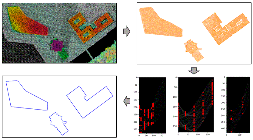
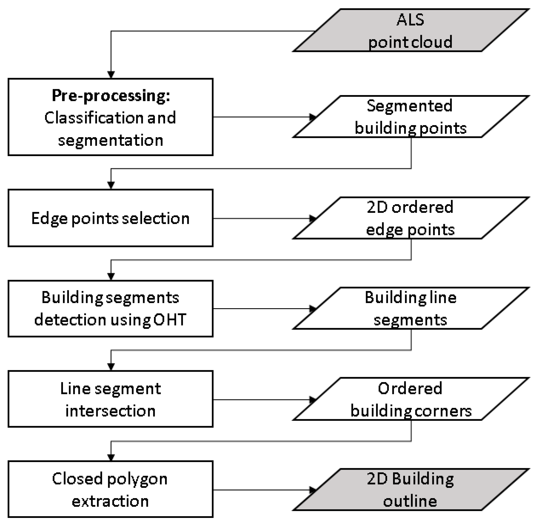
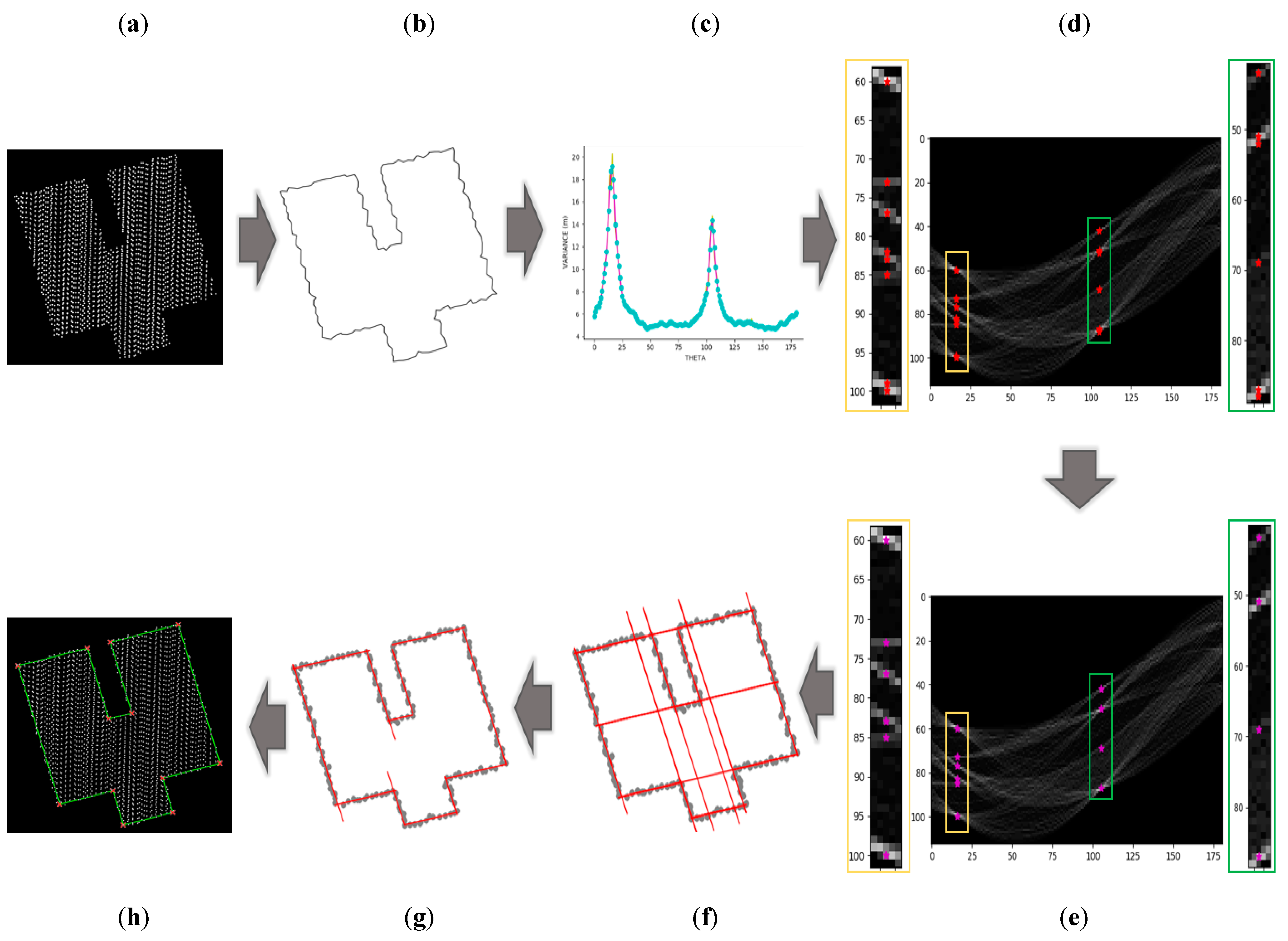
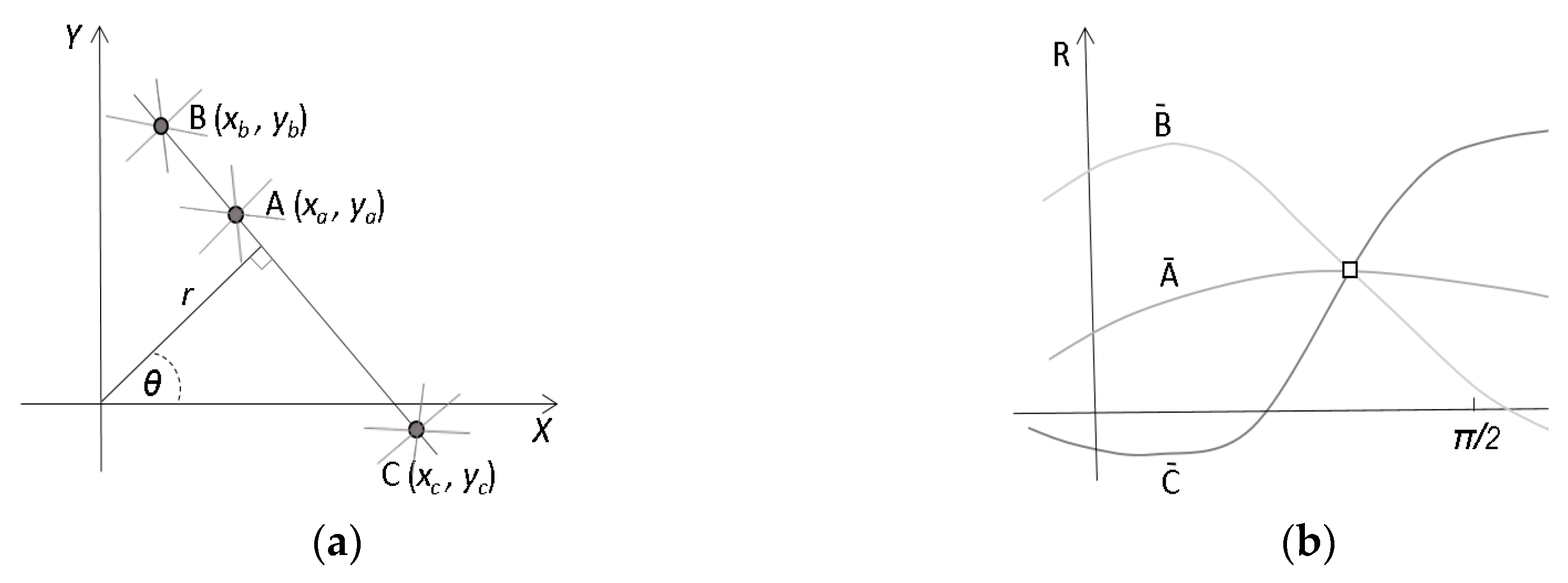
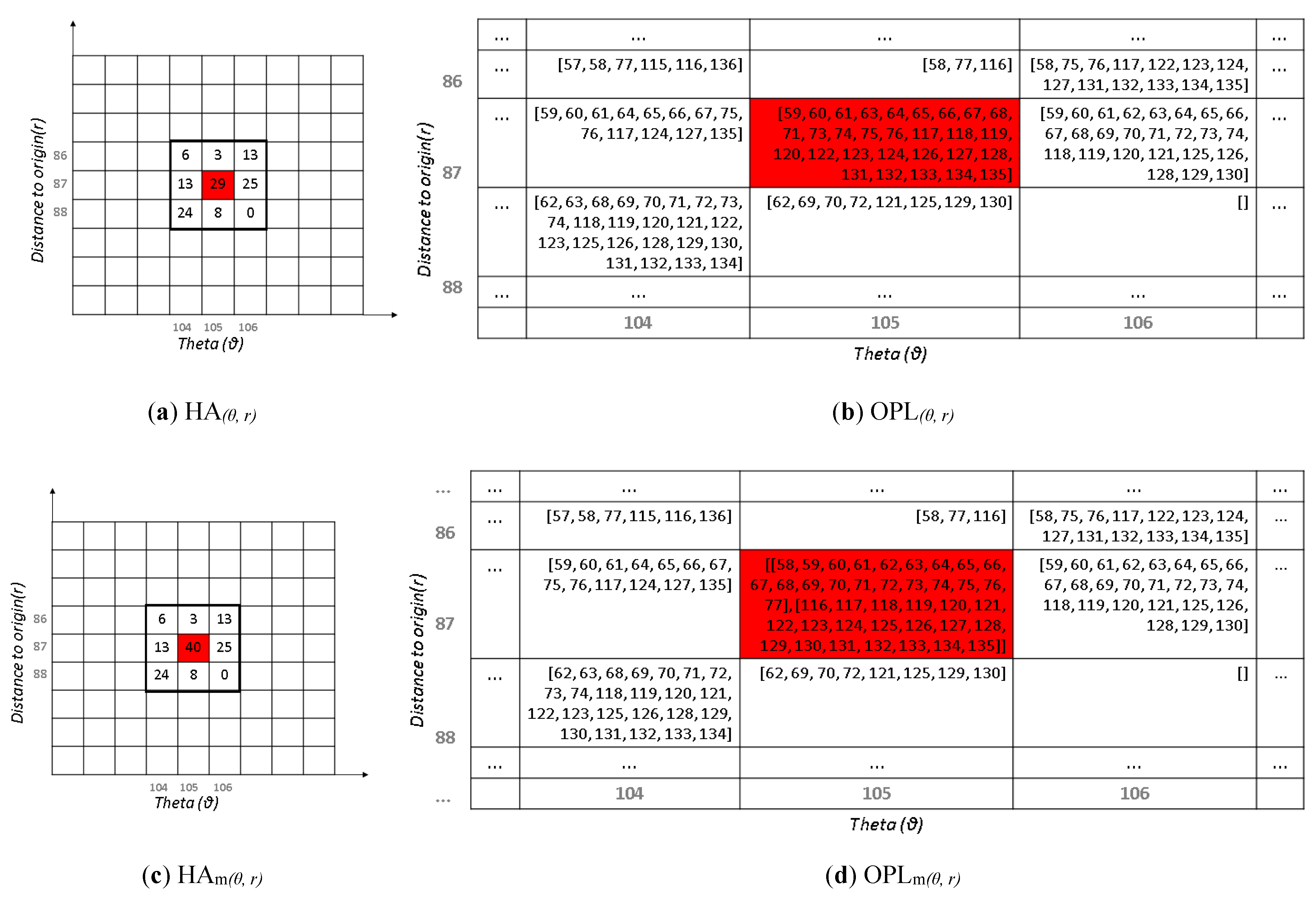
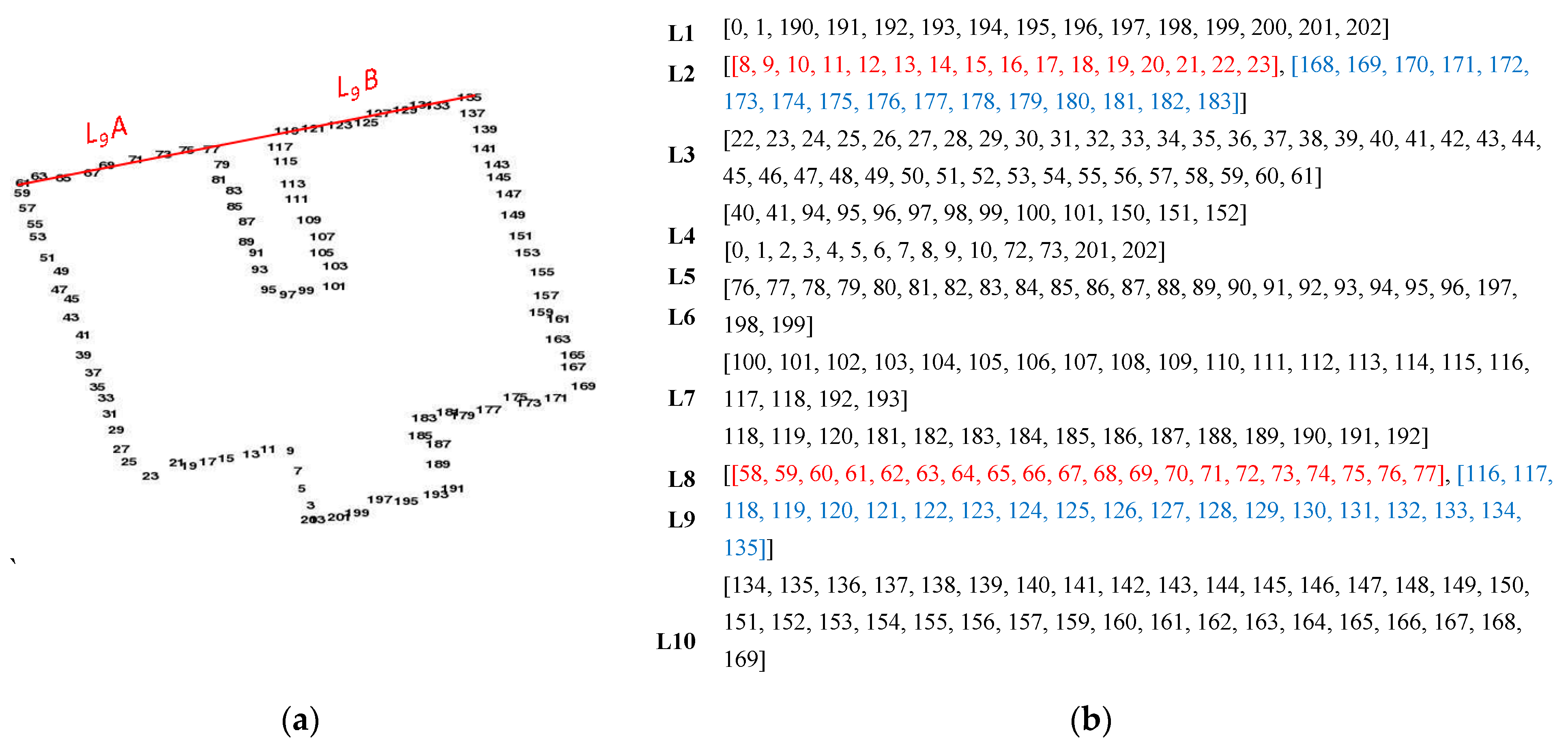
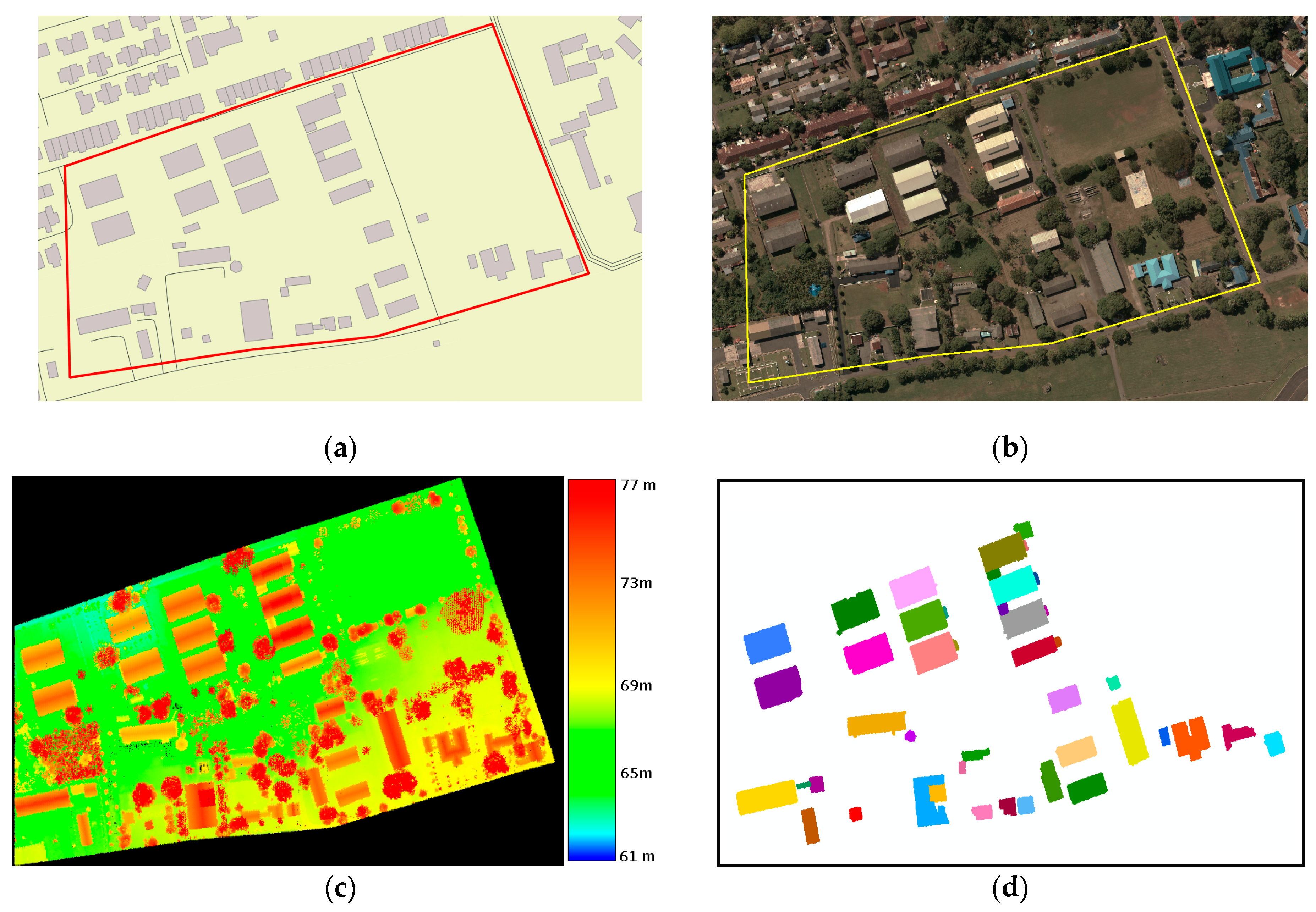
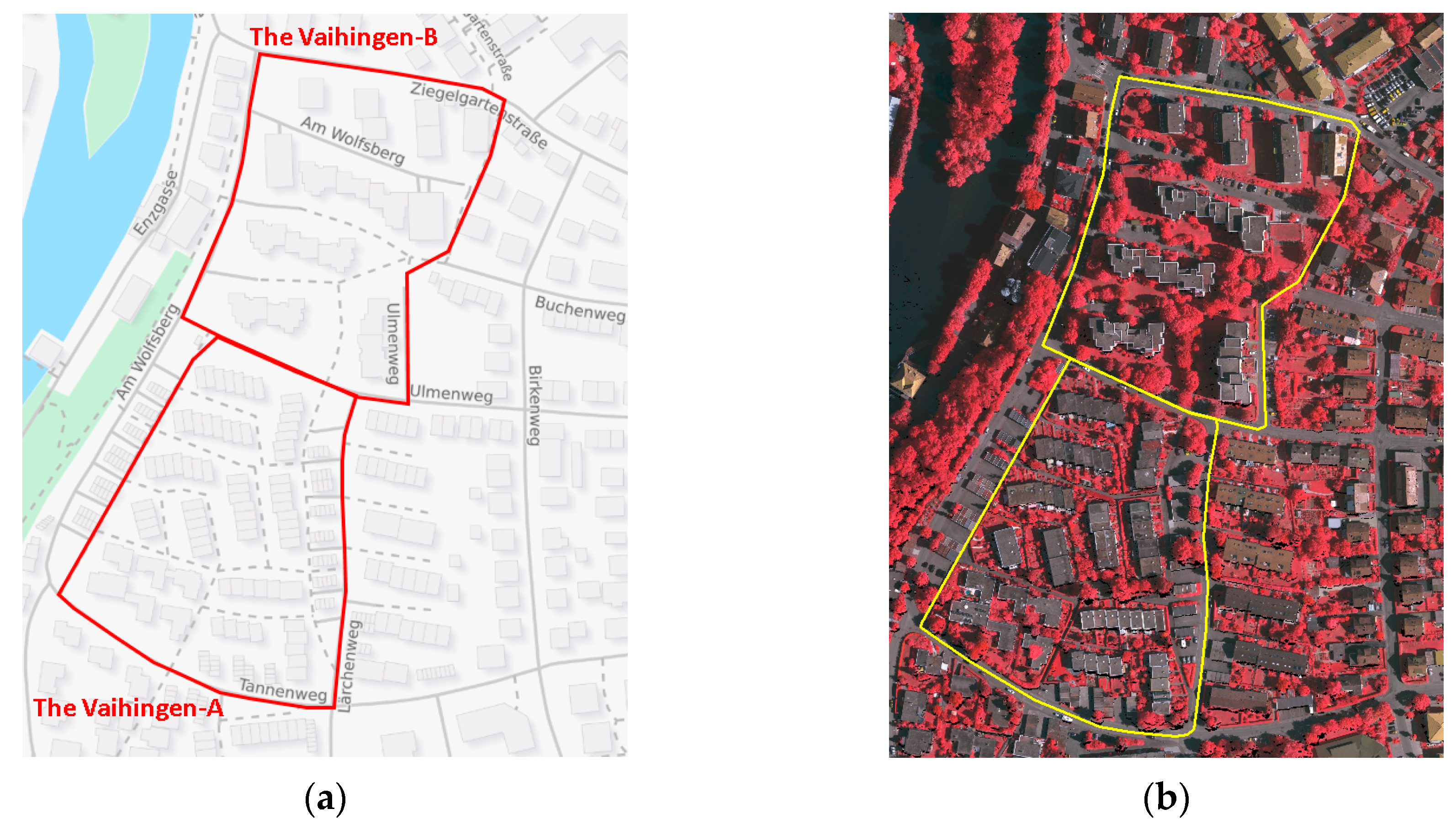
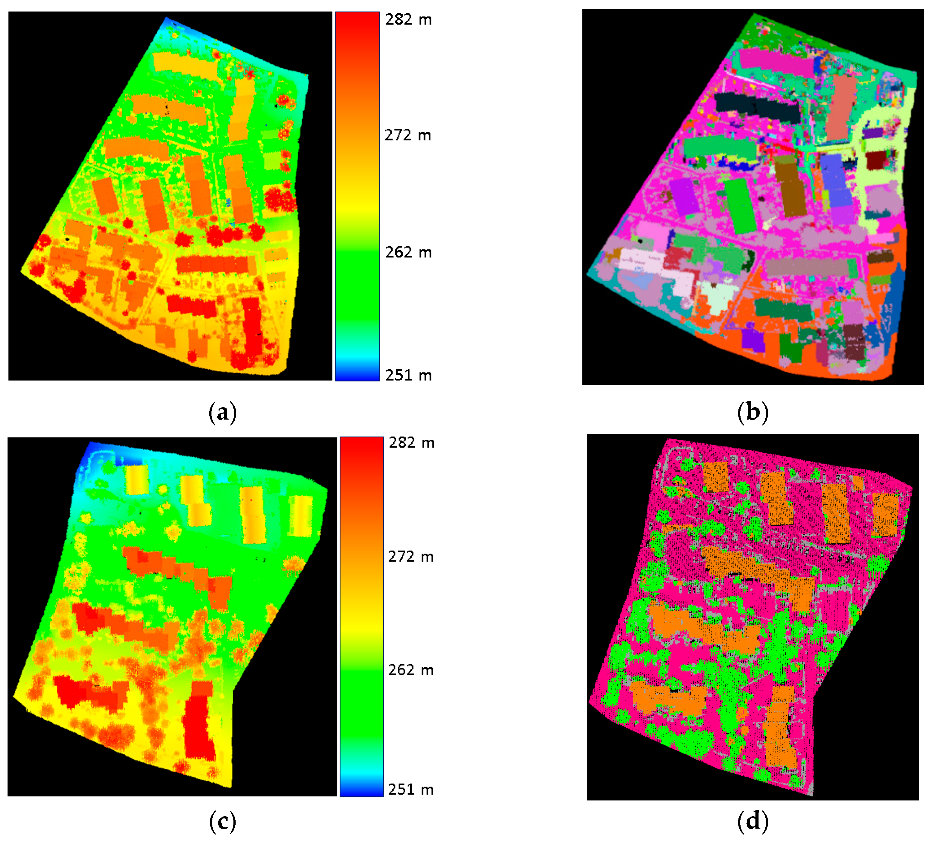
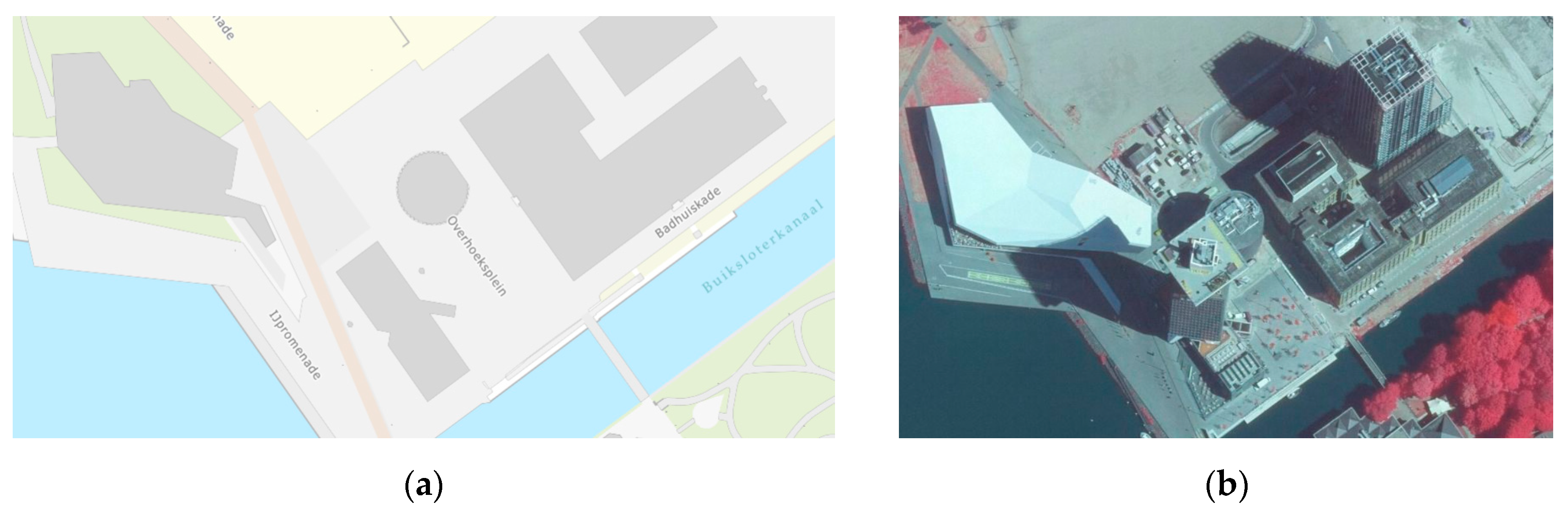
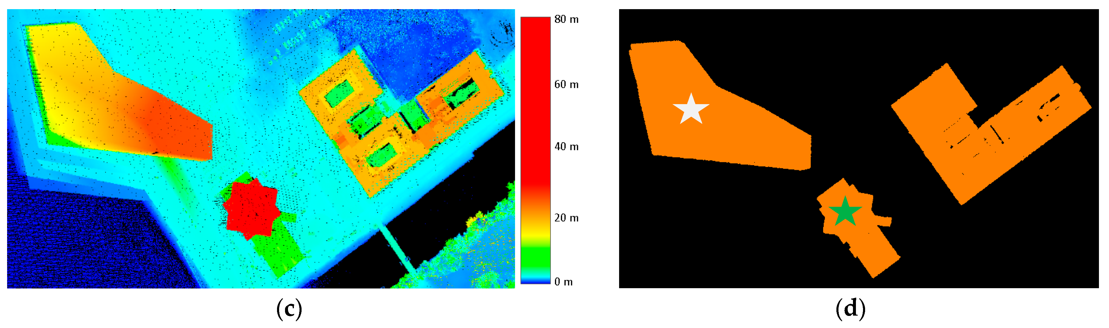
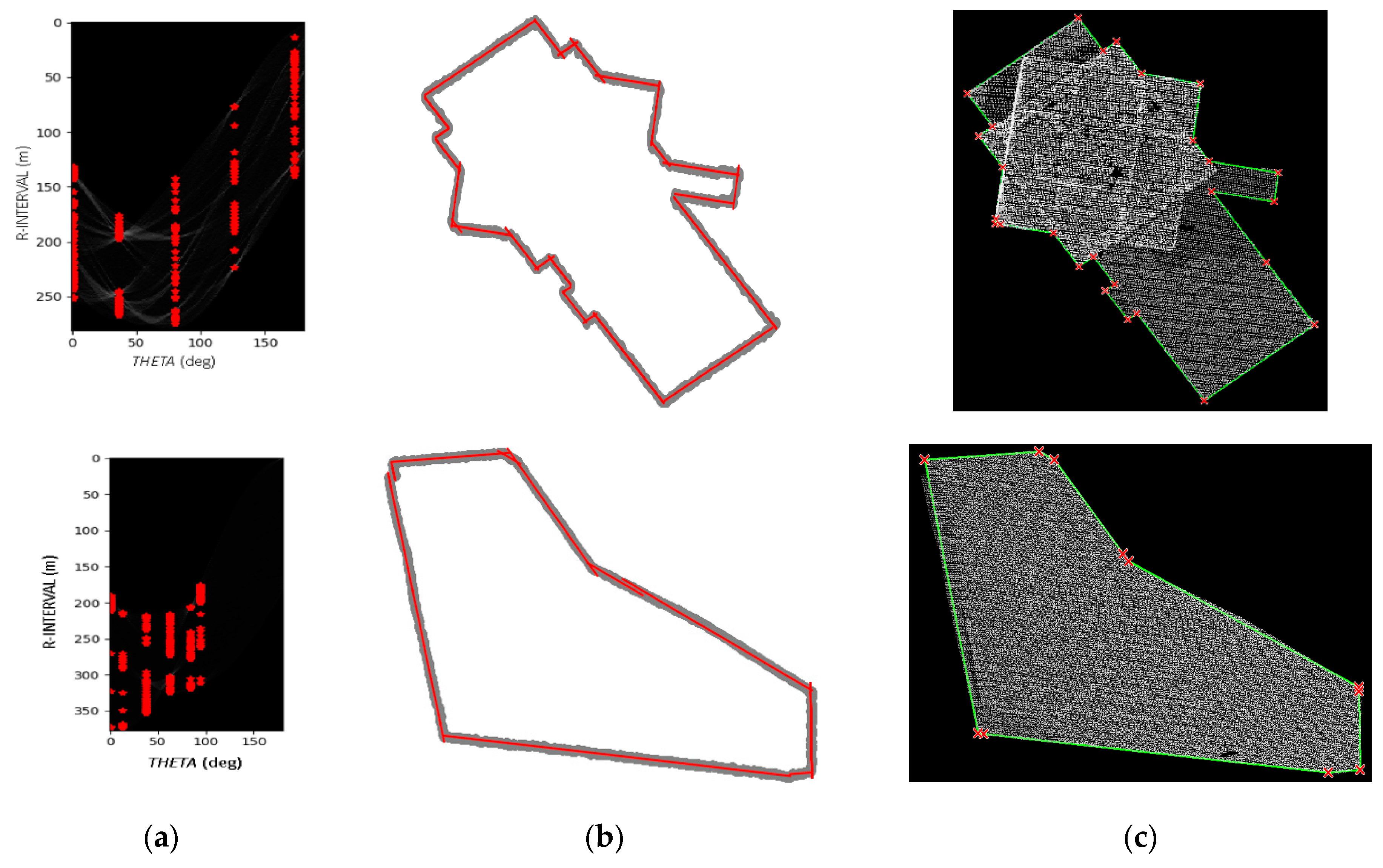
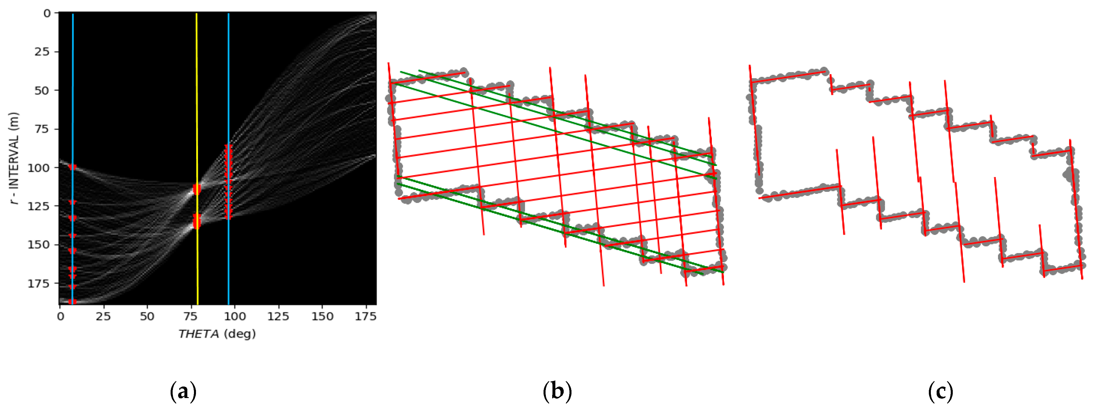
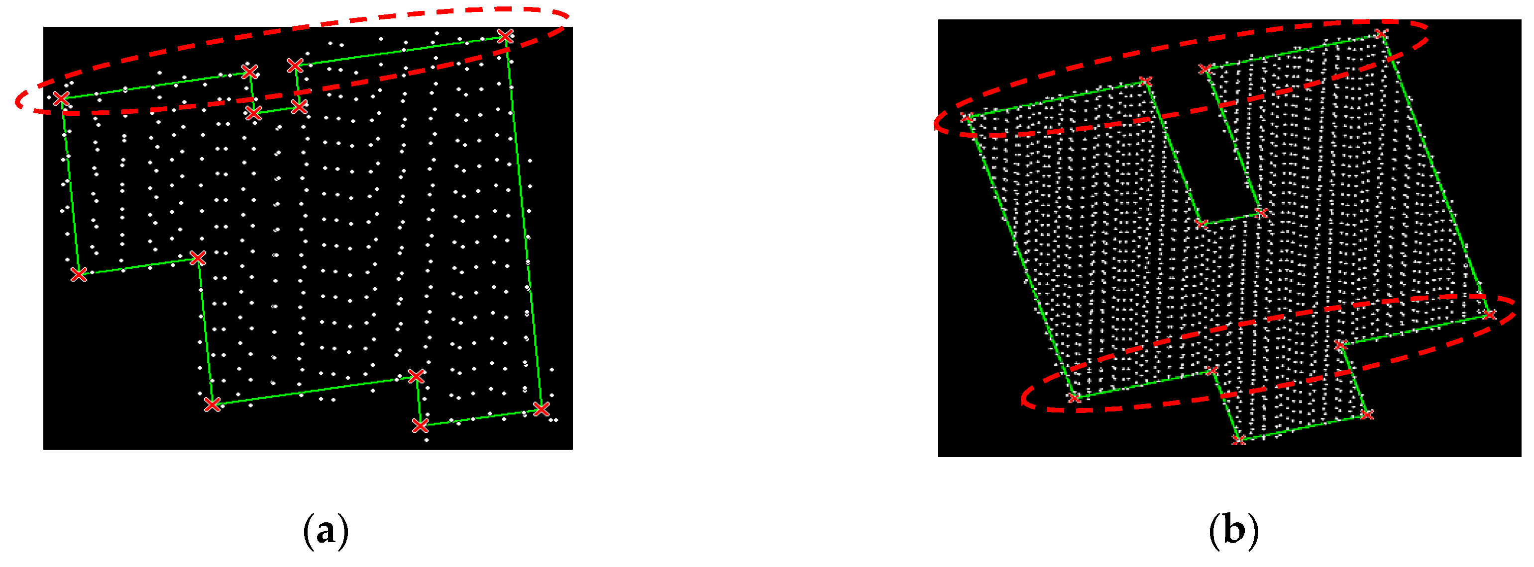
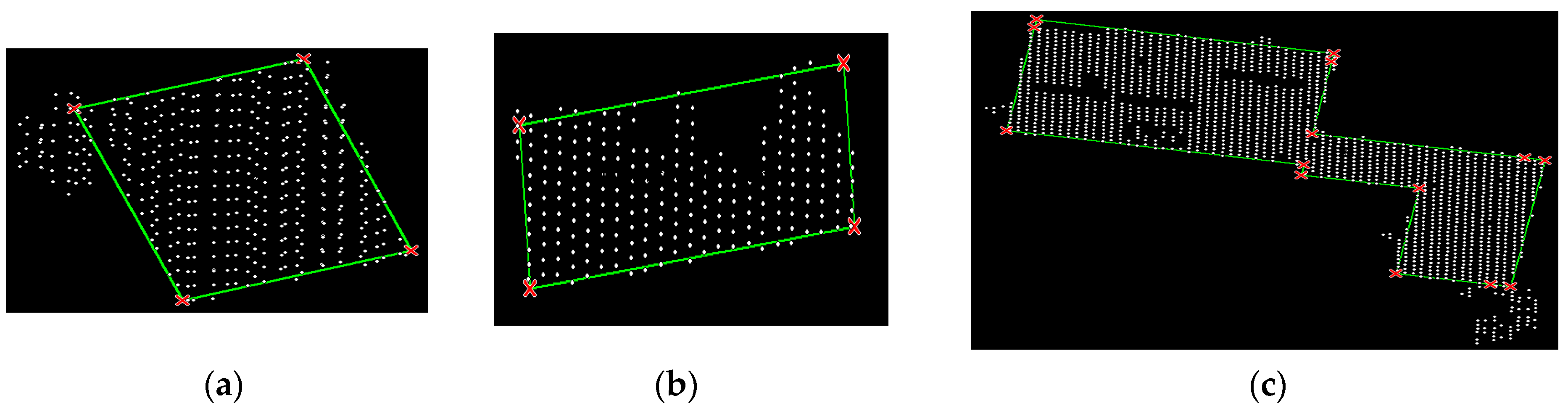
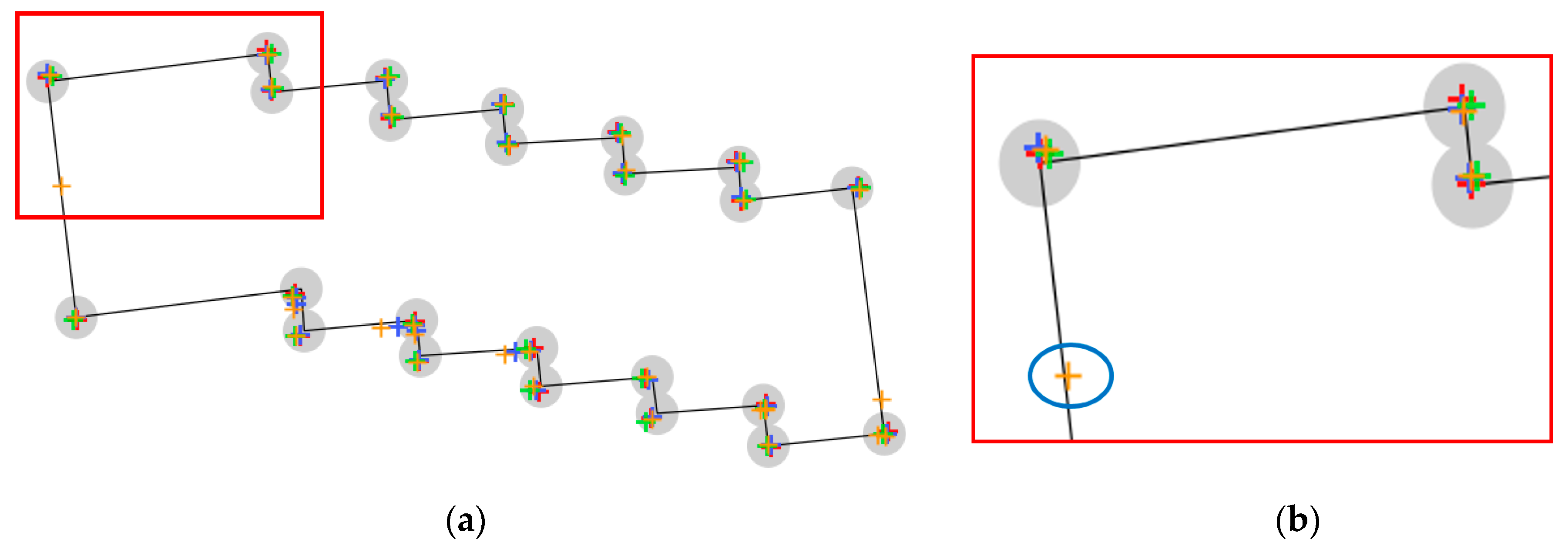
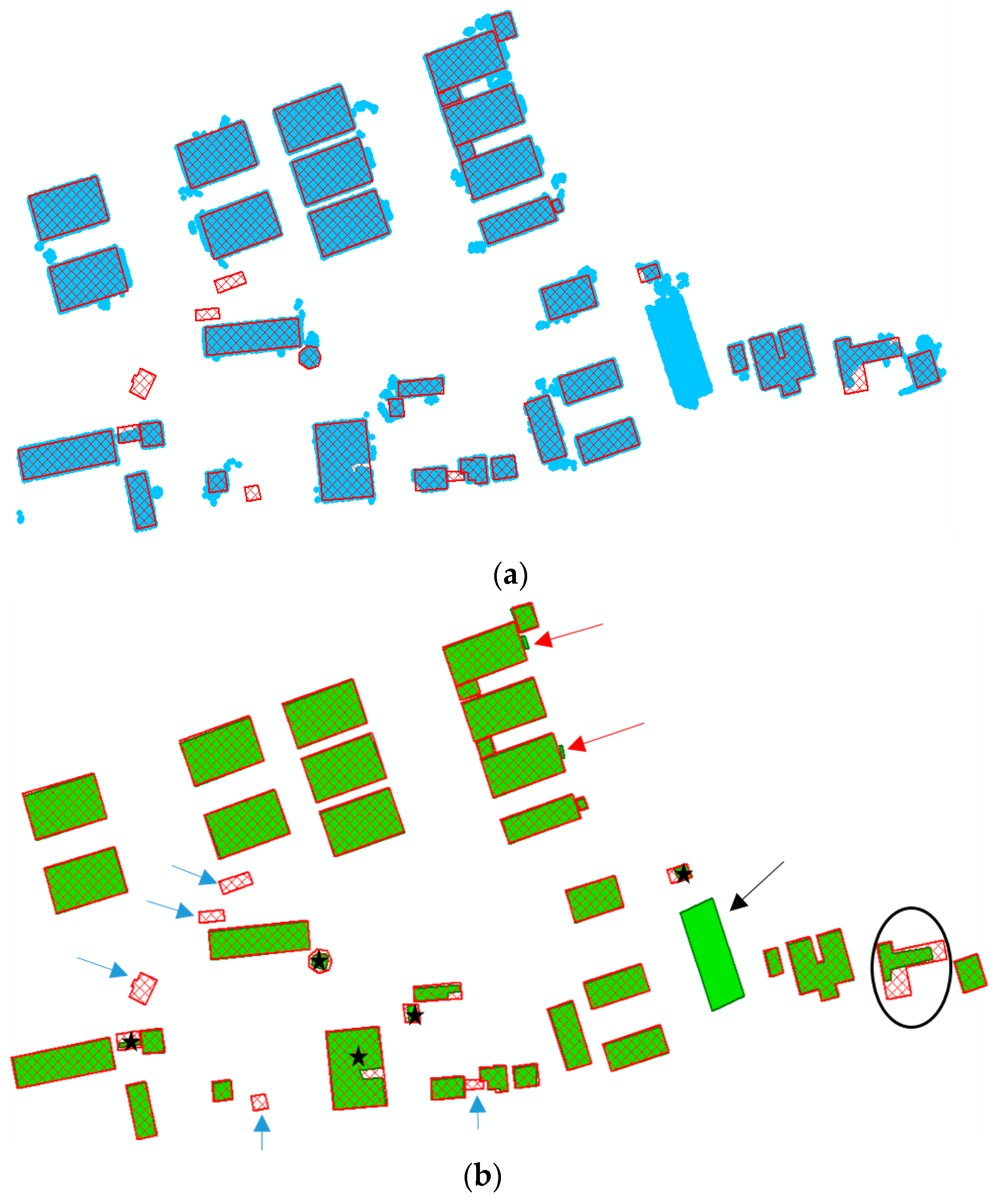
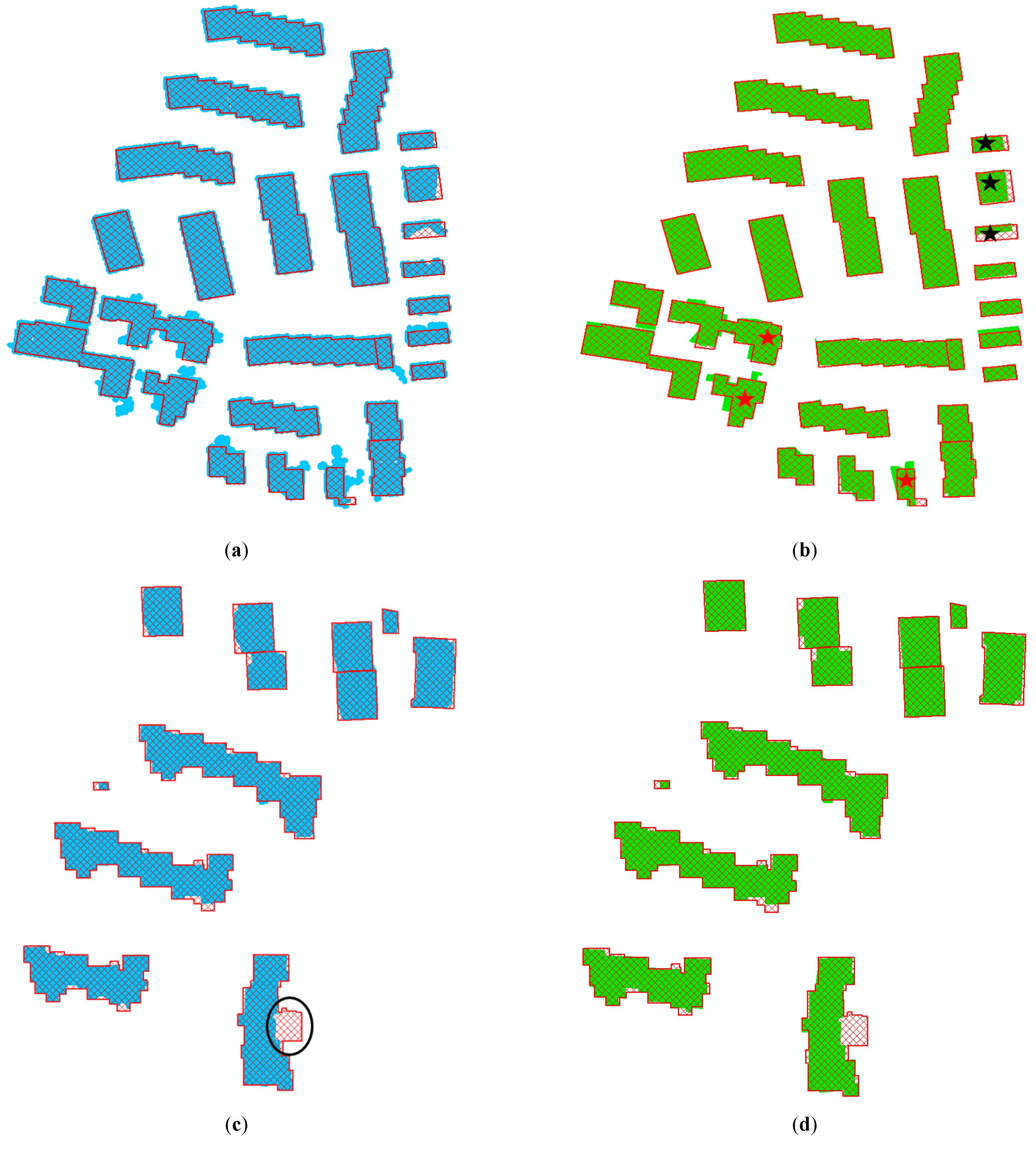
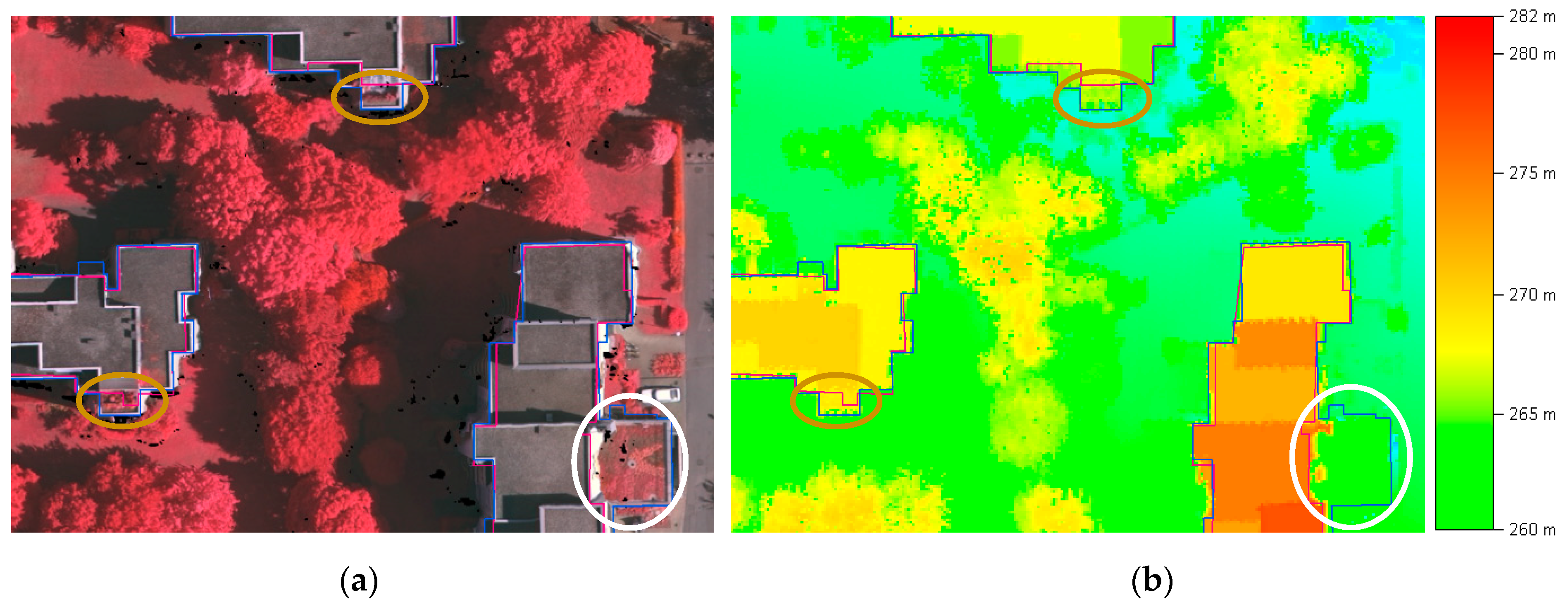
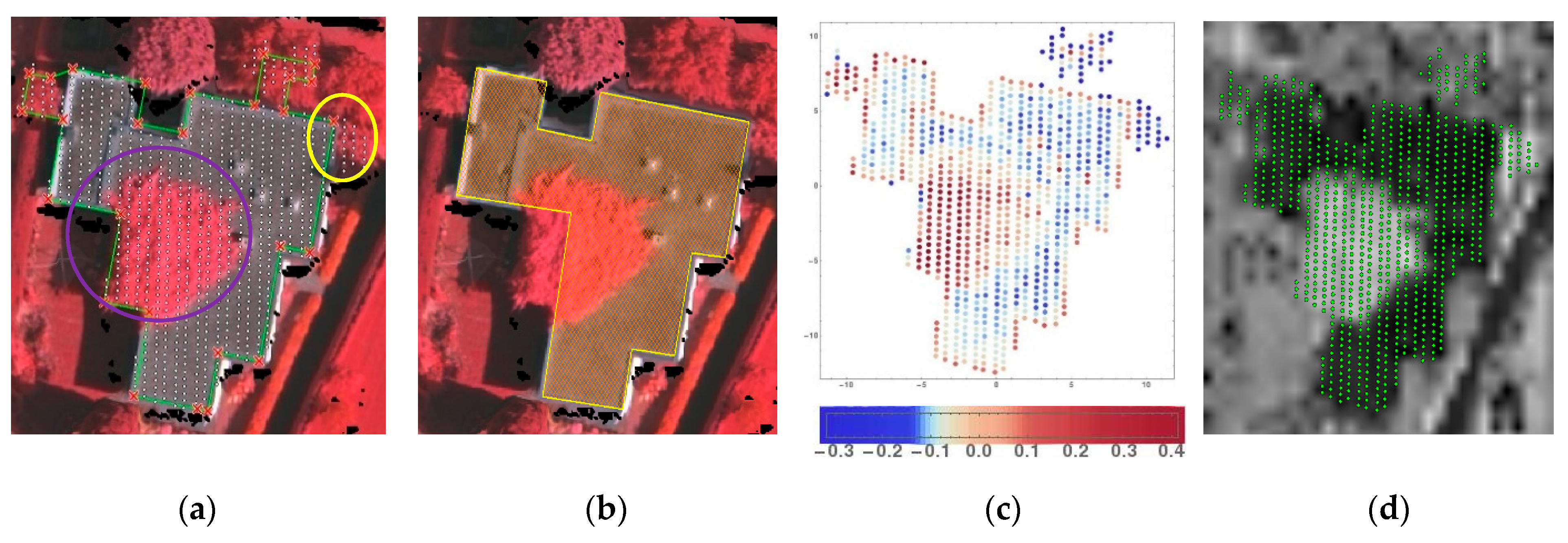
Table 1.
Summary for object representation of different matrix.
| Object Space | Matrix R | Matrix HA | Matrix OPL |
|---|---|---|---|
| Point | Row | Curve | Part of a list |
| Line | Subset of column | Cell/Point | Long list |
| Segment | Sub of subset | Cell/Point | Long list |
Table 2.
Parameter settings for different test sets.
| Test Set | binr | amp | mindist | minL |
|---|---|---|---|---|
| Makassar | 0.3–0.6 m | 0.5 m | 30° | 2.5 m |
| Vaihingen-A | 0.3–0.6 m | 0.15–0.2 m | 15–30° | 1.5 m |
| Vaihingen-B | 0.3–0.6 m | 0.15–0.2 m | 15–30° | 1.5 m |
Table 3.
Evaluation of different bin size.
| Bin Size (cm) | Mean | Std dev | No. of Main Directions | No. of Resulting Segment | No. of Remaining Points | RMSE (m) |
|---|---|---|---|---|---|---|
| Simple Building (four lines/corners) | ||||||
| 20 | 0.071 | 0.043 | 3 | 6 | 5 | 0.224 |
| 40 | 0.126 | 0.105 | 2 | 4 | 0 | 0.206 |
| 50 | 0.121 | 0.101 | 2 | 4 | 0 | 0.198 |
| 60 | 0.167 | 0.161 | 2 | 4 | 0 | 0.223 |
| 80 | 0.223 | 0.195 | 2 | 4 | 0 | 0.248 |
| Complex Building (24 lines/corners) | ||||||
| 20 | 0.086 | 0.059 | 3 | 11 | 62 | N/A |
| 30 | 0.140 | 0.109 | 4 | 17 | 19 | N/A |
| 40 | 0.153 | 0.133 | 3 | 24 | 0 | 0.203 |
| 50 | 0.192 | 0.168 | 3 | 28 | 0 | 0.346 |
| 60 | 0.259 | 0.206 | 3 | 24 | 0 | 0.362 |
| 70 | 0.284 | 0.248 | 3 | 33 | 0 | 0.473 |
| 80 | 0.363 | 0.288 | 3 | 36 | 0 | 0.927 |
| 90 | 0.390 | 0.356 | 3 | 26 | 6 | N/A |
Table 4.
Quality metrics of the building outline results and the concave hull results. (Cp: completeness, Cr: correctness, Q: quality)
Table 4.
Quality metrics of the building outline results and the concave hull results. (Cp: completeness, Cr: correctness, Q: quality)
| Test Set | Building Polygon | Cp (%) | Cr (%) | Q (%) |
|---|---|---|---|---|
| Makassar | OHT results | 91.8 | 99.2 | 91.1 |
| Concave hull | 92.1 | 98.3 | 90.7 | |
| Vaihingen-A | OHT results | 96.4 | 96.5 | 93.2 |
| Concave hull | 95.3 | 95.2 | 90.9 | |
| Vaihingen-B | OHT results | 90.1 | 99.4 | 89.6 |
| Concave hull | 90.9 | 99.6 | 90.6 |
Table 5.
Comparison to previous studies. (Cp: completeness, Cr: correctness, Q: quality)
| Test Set | Input Data | Cp (%) | Cr (%) | Q (%) |
|---|---|---|---|---|
| Awrangjeb, 2014 (MON2) | ALS | 87.1 | 94.0 | 82.6 |
| Siddiqui et al., 2016 (MON3) | ALS + Photos | 97.2 | 84.3 | 82.3 |
| Gilani et al., 2016 (FED_2) | ALS + Photos | 88.8 | 84.5 | 76.4 |
| Zhao et al., 2016 | ALS + Photos | 91.0 | 95.0 | 86.8 |
| Huang et al., 2018 | ALS | 87.3 | 99.0 | 86.5 |
| Proposed method | ALS | 90.1 | 99.4 | 89.6 |
© 2019 by the authors. Licensee MDPI, Basel, Switzerland. This article is an open access article distributed under the terms and conditions of the Creative Commons Attribution (CC BY) license (http://creativecommons.org/licenses/by/4.0/).
Share and Cite
MDPI and ACS Style
Widyaningrum, E.; Gorte, B.; Lindenbergh, R. Automatic Building Outline Extraction from ALS Point Clouds by Ordered Points Aided Hough Transform. Remote Sens. 2019, 11, 1727. https://0-doi-org.brum.beds.ac.uk/10.3390/rs11141727
AMA Style
Widyaningrum E, Gorte B, Lindenbergh R. Automatic Building Outline Extraction from ALS Point Clouds by Ordered Points Aided Hough Transform. Remote Sensing. 2019; 11(14):1727. https://0-doi-org.brum.beds.ac.uk/10.3390/rs11141727
Chicago/Turabian StyleWidyaningrum, Elyta, Ben Gorte, and Roderik Lindenbergh. 2019. "Automatic Building Outline Extraction from ALS Point Clouds by Ordered Points Aided Hough Transform" Remote Sensing 11, no. 14: 1727. https://0-doi-org.brum.beds.ac.uk/10.3390/rs11141727
Note that from the first issue of 2016, this journal uses article numbers instead of page numbers. See further details here.