Comparing Spectral Characteristics of Landsat-8 and Sentinel-2 Same-Day Data for Arctic-Boreal Regions


1
Alfred Wegener Institute for Polar and Marine Research, Telegrafenberg A 45, 14473 Potsdam, Germany
2
Institute of Geosciences, University of Potsdam, Karl-Liebknecht-Str. 24-25, 14476 Potsdam-Golm, Germany
*
Author to whom correspondence should be addressed.
Remote Sens. 2019, 11(14), 1730; https://0-doi-org.brum.beds.ac.uk/10.3390/rs11141730
Submission received: 4 June 2019
/
Revised: 9 July 2019
/
Accepted: 18 July 2019
/
Published: 22 July 2019
(This article belongs to the Section Environmental Remote Sensing)
Abstract
:The Arctic-Boreal regions experience strong changes of air temperature and precipitation regimes, which affect the thermal state of the permafrost. This results in widespread permafrost-thaw disturbances, some unfolding slowly and over long periods, others occurring rapidly and abruptly. Despite optical remote sensing offering a variety of techniques to assess and monitor landscape changes, a persistent cloud cover decreases the amount of usable images considerably. However, combining data from multiple platforms promises to increase the number of images drastically. We therefore assess the comparability of Landsat-8 and Sentinel-2 imagery and the possibility to use both Landsat and Sentinel-2 images together in time series analyses, achieving a temporally-dense data coverage in Arctic-Boreal regions. We determined overlapping same-day acquisitions of Landsat-8 and Sentinel-2 images for three representative study sites in Eastern Siberia. We then compared the Landsat-8 and Sentinel-2 pixel-pairs, downscaled to 60 m, of corresponding bands and derived the ordinary least squares regression for every band combination. The acquired coefficients were used for spectral bandpass adjustment between the two sensors. The spectral band comparisons showed an overall good fit between Landsat-8 and Sentinel-2 images already. The ordinary least squares regression analyses underline the generally good spectral fit with intercept values between 0.0031 and 0.056 and slope values between 0.531 and 0.877. A spectral comparison after spectral bandpass adjustment of Sentinel-2 values to Landsat-8 shows a nearly perfect alignment between the same-day images. The spectral band adjustment succeeds in adjusting Sentinel-2 spectral values to Landsat-8 very well in Eastern Siberian Arctic-Boreal landscapes. After spectral adjustment, Landsat and Sentinel-2 data can be used to create temporally-dense time series and be applied to assess permafrost landscape changes in Eastern Siberia. Remaining differences between the sensors can be attributed to several factors including heterogeneous terrain, poor cloud and cloud shadow masking, and mixed pixels.
1. Introduction
The Arctic-Boreal domain is currently undergoing extensive environmental changes. Mean annual air temperatures increased by up to 1.5–2 C over the 1960–2009 period [1], and precipitation increased, with climate models showing further precipitation increases with additional warming [2]. Both the increase in air temperatures and precipitation also affect the thermal state of permafrost, which is defined as ground that remains at or below a temperature of 0 C for at least two consecutive years and is very widespread in this region [3]. Considering that about a quarter of the Northern Hemisphere is underlain by permafrost, which is 65% of the land north of 60 degrees [4], these changes are of great importance to northern high latitude ecosystems [5]. Continued warming of permafrost across the pan-Arctic region [6] ultimately will result in widespread permafrost thaw and eventually cause near-surface permafrost loss on local to regional scales [7]. Thawing permafrost has direct implications for hydrological systems [8], ecosystems [5], soil carbon decomposition and accumulation [9], greenhouse gas emissions [10], and infrastructure stability in permafrost areas [11]. A multitude of landscape-scale changes, such as active layer deepening, thermokarst and talik formation, soil erosion, and changes in vegetation composition and surface hydrology can be linked to permafrost thaw [12,13,14,15].
While permafrost itself cannot be observed directly with remote sensing, detectable surface disturbance can be linked to permafrost degradation. They can be distinguished between press and pulse disturbances, which are gradual and abrupt disturbance regimes respectively and alter the ecosystem and environment substantially [16]. Press disturbances are driven by impacts and change factors unfolding over decades to centuries and occur gradually and continuously. Press disturbances include processes such as permafrost top-down thaw, as well as vegetation structure and composition changes. They usually occur on extensive regional scales. In contrast to that, pulse disturbances unfold within very short time periods from a few days to years. They are usually extreme in nature and affect the system rapidly as one-time or episodic short-term events, but arise locally in distinct areas. Pulse disturbances include soil erosion, thermokarst lake expansion, lake drainage, and wildfires. Press and pulse disturbances interact with one another as well; for example, press disturbances can trigger pulse disturbances. Exemplary is permafrost top-down thaw initiating rapid thermokarst development or soil erosion [17,18]. To understand the complex feedbacks of permafrost degradation processes and resulting landscape and ecosystem dynamics in space and time, it is critical to track and quantify these not only at the field site scale, but at high spatial resolution across decadal time scales and extensive regions.
Remote sensing provides excellent tools to understand and quantify many of these dynamics linked to surface expressions and land cover changes associated with permafrost degradation across large regions [18,19,20]. For example, Nitze et al. [21] mapped widespread permafrost disturbances based on trend analysis using linear regression on Landsat multispectral index time series, highlighting the abundance and distribution of disturbances such as thermokarst lake changes, wildfires, and thaw slumps. Similarly, Pastick et al. [22] analyzed the diversity of landscape and ecosystem dynamics for Alaska using Landsat-based time series analysis in combination with spectral metrics, climatic data, and topographical and soil information. Using statistical models, they predicted and understood the drivers of change and differentiated between gradual and abrupt disturbances. Apart from understanding the spatial coverage, magnitude, patterns, and dimension of disturbances, the temporal dynamics of disturbances such as initiation timing, duration and persistence, recovery time, and recurrence frequency are highly important parameters for monitoring and projecting Arctic-Boreal ecosystem and landscape trajectories in a changing climate. Space-borne remote sensing with a high temporal and spatial resolution allows detailed monitoring of both gradual and abrupt changes, such as press and pulse disturbances, but requires more detailed insights into the timing and magnitudes of spectral changes of observation targets.
Algorithms developed for monitoring forest disturbances, such as LandTrendr, manage to identify both abrupt and gradual changes with temporally-dense Landsat time series [23]. Likewise, Sulla-Menashe et al. [24] used Normalized Difference Vegetation Index (NDVI) Landsat time series for characterizing vegetation greening and browning patterns in Canadian boreal forests and identified the major driver of the signal to be vegetation recovery following disturbance. Implementing such algorithms developed for boreal ecosystems for extensive monitoring and assessing of disturbance types and dynamics, such as differentiating between press and pulse disturbances, across Arctic-Boreal permafrost regions will improve understanding of climate change and anthropogenic impacts in high latitudes on multiple temporal scales. Most of the schemes so far rely on the extensive Landsat record, which features the longest continuous data archive of optical Earth surface imagery, covering more than 45 years. However, the low temporal resolution of Landsat images and some environmental factors, such as a short growing season length, a challenging solar geometry, frequent snow and ice cover, and especially persistent cloud cover, negatively affect the availability of images for detailed studies [25,26]. Therefore, often, only a rather low number of adequate Landsat images are available for time series analyses in high latitudes. In many regions, these are not sufficient for creating temporally dense time series, which are needed for extracting detailed trends of disturbances and especially their short-term dynamics.
An approach to increase the data base in high latitudes is to combine Landsat time series, which relies on a single platform only, with images from additional optical sensors. A combined data base allows creating temporally much denser time series for the Arctic-Boreal domain, thereby increasing opportunities for monitoring permafrost region disturbances and ecosystem changes. The European Space Agency (ESA) Copernicus Sentinel-2 mission started in 2015 and consists of two satellites (S-2A, S-2B), which have a combined revisit time of five days [27]. Landsat-8 and Sentinel-2’s sensors are both multispectral optical systems, have Sun-synchronous polar orbits, and obtain data with a comparable resolution. Both sensors record multispectral data with bands that cover similar wavelength ranges (Table 1). Sentinel-2 sensors’ similar characteristics to Landsat and shortened revisit time are now leveraging the combined multispectral observation power of three platforms observing the Earth’s surface at 10–30 m resolution, significantly increasing the chance for capturing cloud-free observations at high latitudes. Li and Roy [28] quantified the combined revisit time of Landsat 8, Sentinel-2A, and Sentinel-2B, showing that the global average revisit interval was 2.9 days. With the increased poleward orbit overlap and the enhanced spatial overlap between acquisition swaths, the high latitudes (>70 N) feature the highest number of acquired images within a year (>400 images) and the shortest revisit interval (<1 day) [28]. This dramatic increase in image numbers and shortened revisit time for a combined Landsat-8 and Sentinel-2 time series could facilitate tracking permafrost region disturbances in much higher detail.
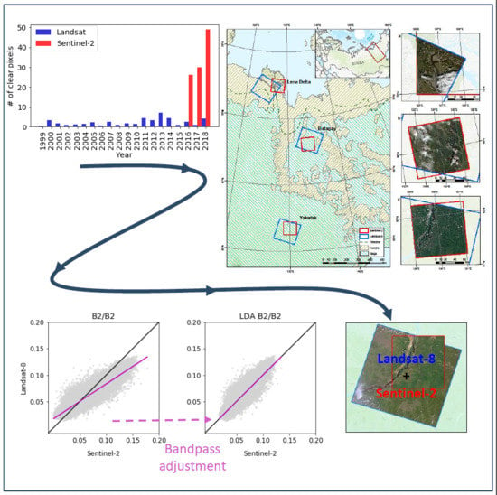
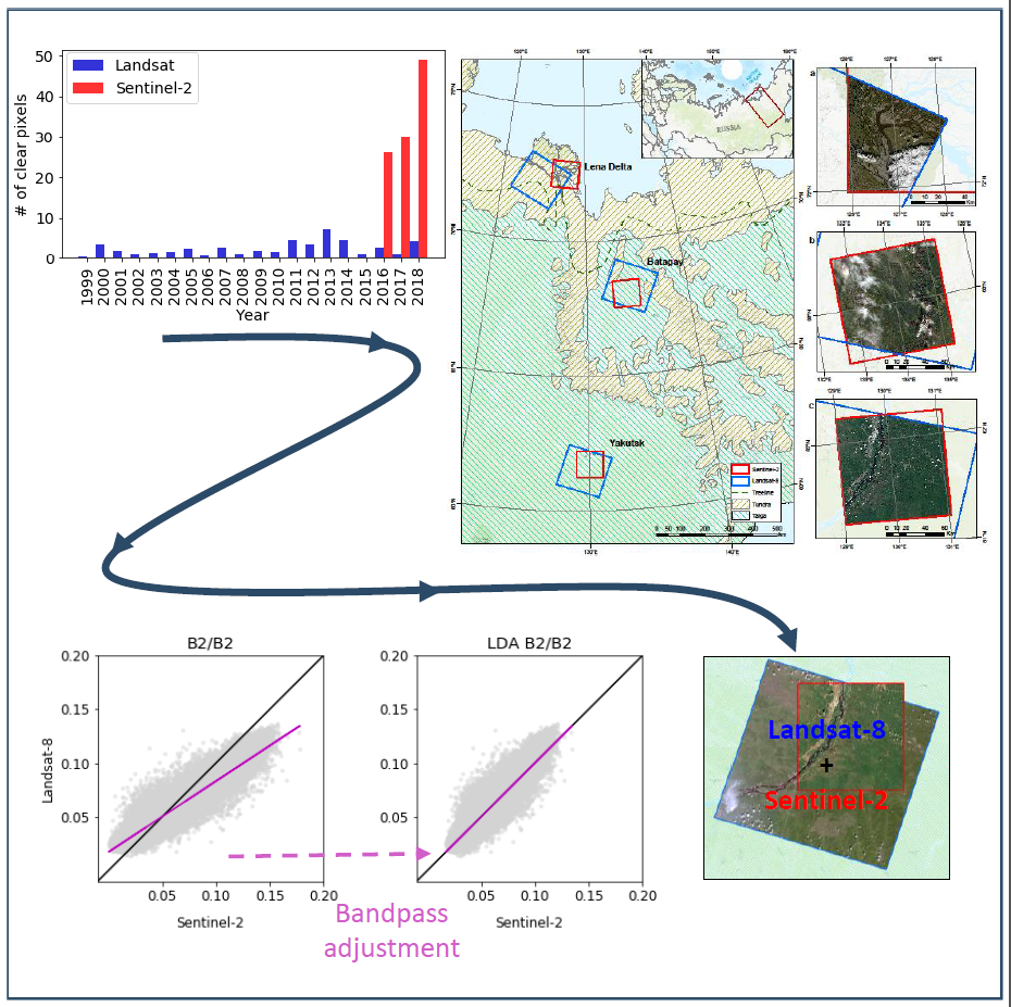
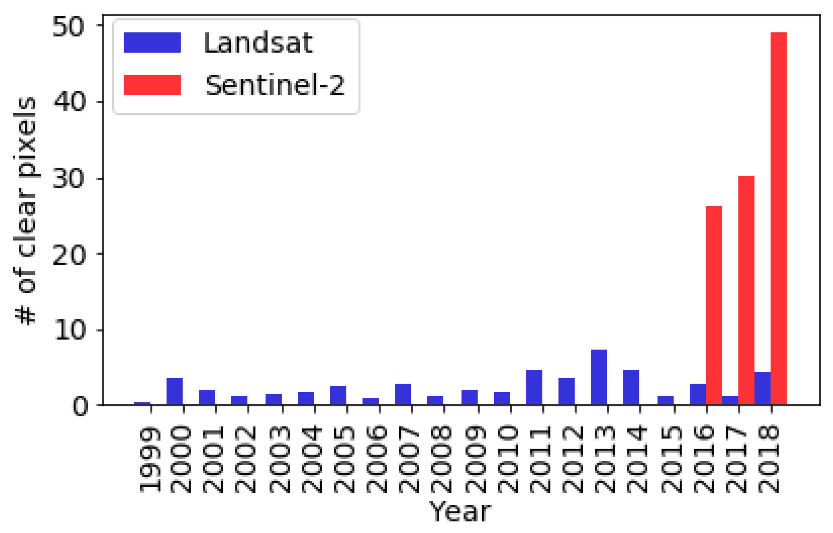
In terms of time series analyses, we do not just require cloud-free images, but rather depend on clear pixels for every location in one study area. A high number of clear pixels available in one observation period (summer months) indicates a good overall data coverage. Figure 1 shows the average number of clear pixels in the Lena Delta (see Section 2.1) for the summer months of every year. It becomes obvious that the average number of clear pixels for every location in the Lena Delta increases dramatically, when adding Sentinel-2 to the analysis. This underlines that relying not only on one sensor platform, but on multiple ones enhances the database drastically.
For a combined time series, it is necessary to align the image products of the different sensors geometrically and radiometrically, ensuring that the same point on the ground is captured with similar spectral reflectance properties in both products. This issue was already addressed for the Landsat sensor series, defining adjustment schemes for slight differences in reflectance measurements, ensuring data continuity and that the Landsat image products from the different sensors (Landsat-5 TM, Landsat-7 ETM+, and Landsat-8 OLI) can be used in a combined time series analysis [29,30,31,32]. To extend the data continuity incentive beyond the Landsat sensors and also to be able to include Sentinel-2, previous studies compared Landsat-8 with Sentinel-2 data and defined bandpass adjustments between corresponding Landsat-8 and Sentinel-2 bands for a better fit. Despite similar wavelength ranges covered by the corresponding bands, the spectral response functions per sensor differ, and this impact has to be assessed before a combined time series is applied [33]. Previous comparison studies varied in application region, scale, input datasets, ranging from simulated to acquired image products, and covered temporally close to same-day acquisitions [33,34,35,36,37]. Regardless of these differences, the comparison approaches are always alike, examining corresponding Landsat-8 and Sentinel-2 bands, comparing pixel-pairs, and deriving regression equations for bandpass alignments. Claverie et al. [38] conducted a comparison between Landsat-8 and Sentinel-2 data for 91 test sites worldwide and created a globally-applicable Harmonized Landsat and Sentinel-2 surface reflectance dataset (HLS). While a few sample sites are situated in Alaska, Canada, and Northern Scandinavia, sites from the Siberian high latitudes are not included. Flood [39] was first to compare same-day Landsat-8 with Sentinel-2 acquisition pixel-pairs of corresponding bands for Australia and defined band-wise adjustment equations. Furthermore, Flood [39] applied the global HLS bandpass correction to the same dataset, but concluded that the HLS adjustment did not sufficiently adjust the Sentinel-2 data to Landsat-8 data. As a consequence, their region-specific derived bandpass adjustments showed a better fit than the HLS adjustment. An overall result of the previous studies was that Landsat-8 and Sentinel-2 data were comparable, but for a combined analysis, the datasets have to be adjusted to avoid detecting change because of a bias between sensors and not because of changes on the ground, which is particularly important for studying trends. Despite the effort of creating a globally-applicable harmonized product [38], local to regional studies showed that locally-derived bandpass adjustments are superior to the HLS product [34,39]. Therefore, it is recommendable to create region-specific adjustments between Landsat-8 and Sentinel-2 for regional assessments and applications.
So far, to the best of our knowledge, no comparison of Landsat-8 and Sentinel-2 data or an assessment of a potential combined use in time series analyses for the Siberian Arctic-Boreal region has been done. The overall objective of this paper is to compare the spectral characteristics of Landsat-8 and Sentinel-2 data across different types of landscapes and ecosystems in the study domain and assess their compatibility in Arctic-Boreal permafrost regions for the potential use in combined time series. To address this objective, we focus on three sub-objectives: (1) comparison of the spectral characteristics of corresponding bands from Landsat-8 and Sentinel-2 data of same-day acquisitions for three individual study sites in Eastern Siberia that broadly differ in ecosystem and land cover characteristics; (2) defining spectral band adjustments between Landsat-8 and Sentinel-2 data for each of the three study sites; and (3) determining a set of spectral band adjustments that is applicable to Eastern Siberia generally and comparing them to the application of the global Harmonized Landsat Sentinel-2 product.
2. Materials and Methods
2.1. Study Sites
For this assessment, we included three study sites that are representative for the range of land cover conditions in Eastern Siberia: the arctic central Lena Delta (73 N, 126 E), the mountainous Batagay region in the Yana Highlands (67 N, 134 E), and the boreal Maya-Yakutsk region in central Yakutia (62 N, 129 E). The three sites are located along an approximate north-south transect and exemplify the different climatic, geologic, geomorphologic, and vegetational conditions of the quite heterogeneous Eastern Siberian permafrost landscapes, bridging from arctic to boreal regions and covering both tundra and taiga biomes (Figure 2).
The Lena Delta has a maritime-influenced polar tundra climate and is located in Northern Siberia at the Laptev Sea coast, within the continuous permafrost zone. It is the biggest Arctic delta with about 29,000 . The land cover in the delta is dominated by Arctic tundra that varies in vegetation composition between three major geomorphological terraces [40]. We here focused on the central part of the delta where the Arctic research station Samoylov is located [41]. Samoylov Island is one of the 1500 delta islands and part of the first river terrace. The first terrace formed during the Holocene and is characterized by low-center ice-wedge polygonal tundra, polygonal ponds, large thermokarst lakes, and active flood plains [41]. Wet and moist tundra dominates this area with a vegetation cover of sedge, grass, moss, and dwarf shrub wetlands [40]. The study area extends further to the adjacent Kurungnakh Island, which is part of the third terrace, an old late Pleistocene accumulation plain dissected by delta channel formation and thermokarst processes and characterized by polygonal microrelief and thermokarst ponds and lakes [42,43]. The second terrace of the Lena Delta consisting of late Pleistocene fluvial deposits is restricted to the northwestern part of the Lena Delta and is therefore not represented in the study area. From 1999–2011, the mean annual air temperature of the central Lena Delta was −12.5 C with a mean temperature range from 10.1 C–−33.1 C in July and February, respectively. In the same period summer, precipitation ranged from 52 mm (2001) to 199 mm (2003) [41].
The Batagay study area represents a highly continental region with strong seasonal air temperature ranges and an overall low mean annual precipitation [44,45]. Batagay is located at the Yana River and in between the Verhoyansk and Chersky Ranges in the Yansk Uplands, a region that features the cold pole of the Northern Hemisphere and is underlain by continuous permafrost with shallow active layer depths from 0.2–1.2 m [46]. The mean air temperature in July is 15.5 C and in January −44.7 C, while the mean annual precipitation is only 181 mm [45,46]. The land cover in this study area is dominated by light coniferous forests with larch (Larix gmelinii), Siberian dwarf pine (Pinus pumila), and a dense shrub layer. A thick layer of lichens and mosses covers the mostly wet ground [44]. Other portions of the study area consist of barren bedrock surfaces. Ashastina et al. [44] described the bedrock geology as a mix of dark grey siltstone and mudstone that contain layers of sand and clay deposits based on maps and Kunitsky et al. [47]. The Batagay megaslump, the largest known retrogressive thaw slump with a total area of >70 ha and headwall retreat rates of up to 30 m per year in 2016 [48], is located within this study area at about 67 N, 134 E [49]. This large thaw landform indicates the presence of vulnerable ice-rich permafrost as a thick cover deposit in some parts of this region.
The Yakutsk study area in central Yakutia has an extremely continental climate with a mean annual air temperature of −10.2 C, mean January temperatures of −42.6 C, July temperatures of 18.7 C, and an annual precipitation of about 234 mm [50]. The region is dominated by boreal summer green needle forests, mainly by Larix [51]. Ice-rich late Pleistocene permafrost, as well as vegetated dune fields are widespread on the Lena river terraces. Silty clays, sandy silts, and silty sands dominate the Quaternary sediments. Thermokarst lakes and basins dominated by meadow vegetation (alases) are abundant [50,52]. Intensive thermokarst development in the area can reach surface subsidence rates of 5–10 cm per year, and thermokarst lakes more than doubled their area during the 1992–2012 period [50]. The region is also regularly affected by forest fires [53], resulting in a heterogeneous land cover with different disturbance and succession stages of the vegetation.
2.2. Data
In our study, we focused on imagery from Landsat-8 and Sentinel-2. The USGS Landsat-8 satellite was launched in 2013 and is equipped with the Operational Land Imager (OLI) sensor, which is a multi-spectral imager. The satellite has a 16-day repeat cycle, orbiting Sun-synchronously at 705 km altitude. The sensor field of view is 15 degrees, which results in a 185-km swath width. The satellite is also equipped with a co-registered Thermal Infrared Sensor (TIRS) that contains two thermal spectral bands with a ground spatial resolution of 100 m. The nine spectral bands of the OLI sensor have a spatial resolution of 30 m. The Landsat-8 OLI continues the Landsat mission that originally started in 1972 [25]. The ESA Copernicus Sentinel-2A and 2B satellites were launched in 2015 and 2017, respectively, and have the Multi-Spectral Instrument (MSI) aboard, which is also a multi-spectral imager, orbiting at a 786-km altitude Sun-synchronously. The increased orbit altitude together with a field of view of 20.6 degrees results in a swath width of about 290 km. Both Sentinel-2 satellites have a repeat cycle of 10 days, but as they operate out of phase, they have a joint revisit time of five days. The 13 spectral bands of the MSI have different spatial resolutions, 10 m, 20 m, and 60 m (Table 1) [27,54].
We accessed and processed both Landsat-8 and Sentinel-2 imagery predominantly on the Google Earth Engine (GEE) platform. GEE is a cloud-based platform that incorporates analysis-ready data catalogs allowing the user to access and analyze data easily. GEE hosts the entire multi-petabyte Landsat archive, as well as data from Sentinel-2 [55]. The images are ingested and cut into tiles for efficient collection handling in GEE, but remain stored with their original projection, resolution, and bit depth. For this study, we used the “USGS Landsat 8 Surface Reflectance Tier 1” image collection. The images in this collection are atmospherically corrected to surface reflectance based on the Landsat 8 Surface Reflectance Code (LaSRC) and already contain a mask for clouds, shadows, waters, and snow, derived from the CFMASK algorithm [56,57]. For Sentinel-2, we accessed the image products in two ways. First, we selected the “Sentinel-2 MSI: Multi-Spectral Instrument, Level-1C” image collection in GEE, containing Top-Of-Atmosphere (TOA) reflectance images, the only full Sentinel-2 collection provided in GEE at the time. The datasets contain the QA60 band that includes cloud mask information as pre-processed by ESA [54]. We used the GEE Sentinel-2 collection for preparing the filtering and masking step (Step A) as described in Section 2.3.1 and Figure 3. Based on the GEE filtering results, we downloaded the Sentinel-2 Level-1C images from the ESA Copernicus Open Access Hub to process them to surface reflectance data with ESAs’ Sen2Cor atmospheric correction processor that corrects Sentinel-2 Level-1C orthophoto products to Level-2A surface reflectance products (see Section 2.3.3) [58,59]. After processing, we ingested the atmospherically-corrected Sentinel-2 Level-2A images into GEE to continue with Step C of the workflow (Figure 3).
2.3. Data Processing
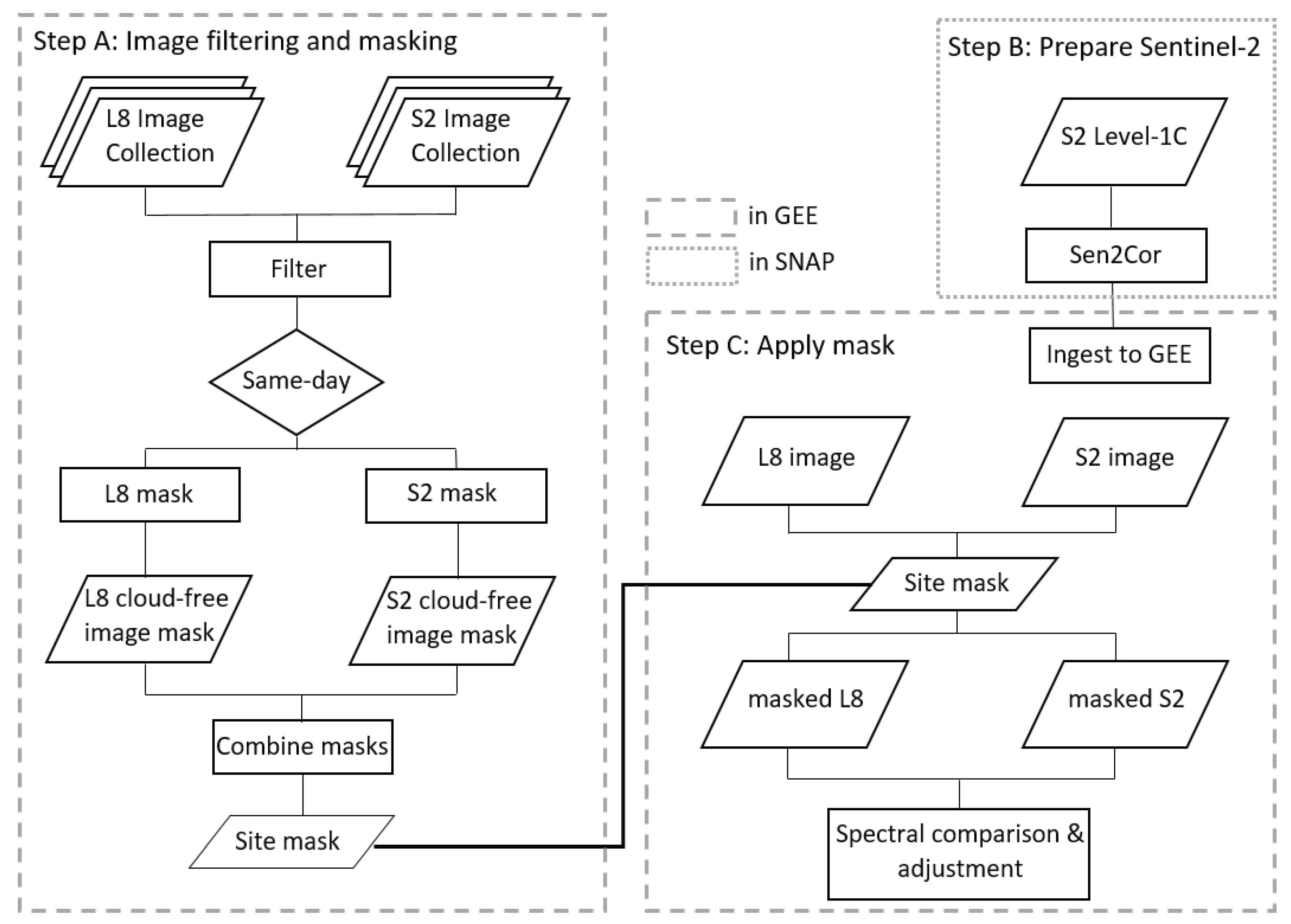
The data processing workflow consisted of three steps (Figure 3). In Step A, we filtered and cloud-masked the imagery. In Step B, we processed Sentinel-2 surface reflectance images with the Sentinel Application Platform. In Step C, we masked the Landsat-8 and Sentinel-2 images to prepare the pixel-by-pixel data input for the spectral comparison and adjustment.
2.3.1. Filtering Image Collections
For each study area (Lena Delta, Batagay, and Yakutsk), we filtered the Landsat-8 and Sentinel-2 GEE image collections based on location, date range, and maximum cloud coverage. We filtered the collections for the Arctic summer months (1 July–31 August 2016) and a maximum cloud cover of 80% per image. We then identified same-day acquisitions of overlapping Landsat-8 and Sentinel-2 images for each study site (Figure 2, Table 2, and Table A1 with the GEE image names). For each study site, we identified one Landsat-8 and one Sentinel-2 image that overlapped substantially and had as little cloud cover as possible. We assumed that there was no change on the ground target between the Landsat-8 and Sentinel-2 identified same-day observations since both satellites are Sun-synchronous with mid-morning overpass times, the same-day acquisitions being taken only minutes apart. Likewise, atmospheric conditions were also expected to not have changed significantly between the acquisitions. Additionally, the solar zenith and solar azimuth angles were very similar and only diverged slightly (Table 2). Therefore, any differences found between the Landsat-8 and Sentinel-2 same-day acquisitions were considered differences in sensor responses exclusively.
2.3.2. Creating L8, S2, and Site Masks
Our method was solely based on a clear pixel comparison. In this case, we defined clear pixels not to contain clouds, cloud shadows, water, or snow, and hence, their surface reflectance values were uncontaminated by these environmental properties. The masking of clouds, cloud shadows, and snow was done in GEE. For Landsat-8, we used the provided “pixel_qa” band that contains cloud, shadow, snow, and water masks derived with the CFMask algorithm [57]. Based on the CFMask information in the “pixel_qa” band, we selected clear pixels only and created a “clear pixel” mask for each Landsat-8 image of the three study sites (L8 mask). For Sentinel-2, we applied a simple cloud score algorithm that uses band thresholds as cloud filtering steps [54]. We also included a cloud shadow shift algorithm taking into account the average cloud height and projecting the estimated cloud shadow based on the cloud position, a GEE code fragment introduced by Donchyts [60]. With this method, we also created a mask for each Sentinel-2 image that selects only clear pixels of that image, creating a “clear pixel” mask (S2 mask).
To identify clear pixels in both datasets, we joined the two masks. First, we reprojected both L8 and S2 clear pixel masks (L8 masks and S2 masks) to the same projection, taking the Landsat-8 image projection as the default projection (WGS 84/ UTM zone 51 N, 52 N, or 53 N for the different study sites). Additionally, we resampled the S2 masks to 30-m spatial resolution to fit to the Landsat-8 resolution. GEE offers a resampling algorithm for images called “reproject”. This algorithm requires two input parameters and then performs nearest neighbor resampling. Firstly, one needs to specify the projection to be used and secondly the desired scale or better spatial resolution in meters of the output image. Then, the L8 mask and S2 mask (30 m) for each image pair per study site were combined. The result was a single mask that contained only overlapping clear pixels from the Landsat-8 and Sentinel-2 same-day acquisitions for every study site (“site mask”).
2.3.3. Preparing Sentinel-2 Surface Reflectance Images in SNAP
We downloaded the same-day Sentinel-2 Level-1C images from ESA’s distribution platform Copernicus Open Access Hub. The images were processed in SNAP to Sentinel-2 Level-2A surface reflectance images with the Sen2Cor tool. Sen2Cor can be run from the Sentinel Application Platform (SNAP) desktop toolbox. We used SNAP Version 6.0.5 including the Sentinel-2 Toolbox (S2TBX) Version 6.0.2 with Sen2Cor Version 255. The input for the Sen2Cor tool is the Sentinel-2 Level-1C image and processing parameters. We defined the processing resolution to 10 m, the aerosol input for the Lena Delta as “Maritime” and for Batagay and Yakutsk as “Rural”, and the type of atmosphere as “mid-latitude summer”, and the remaining parameters were kept as default. The results were Sentinel-2 Level-2A image products, corrected to surface reflectance. After exporting the images as Geotiffs from SNAP, we ingested them into GEE.
2.3.4. Applying Site Masks
The final processing step included the surface reflectance image products. For the L8, we again relied on the image collection “USGS Landsat 8 Surface Reflectance Tier 1” available in GEE. For S2, we used the SNAP-processed Sentinel-2 Level 2A images newly ingested into GEE. To avoid errors due to georeferencing differences, we reprojected the same-day surface reflectance images to the same projection, as described in Section 2.3.2, and resampled the images uniformly to 60-m spatial resolution with an averaging algorithm. The resampling ensured that the Landsat-8 and Sentinel-2 pixel-pairs covered the same ground target [61], in addition to their already good relative co-registration of <6.6 m [62]. Even residual geolocation errors of Landsat-8, which can lead to geographic misalignments between Landsat-8 and Sentinel-2 of up to 38 m, were then reduced [63]. The overall mask per study site (“site mask”) was also resampled to 60 m and then applied to the Landsat-8 and Sentinel-2 surface reflectance (60 m) images. The resulting masked images were now clipped to the site masks’ extent and only contained the corresponding Landsat-8 and Sentinel-2 cloud-free pixels of the same-day acquisitions per study site. The obtained Landsat-8 and Sentinel-2 surface reflectance pixel-pair dataset from the same-day acquisitions was then used as the input for the spectral band comparison and adjustment.
Both the cloud and especially cloud shadow masking were not very reliable, neither for the Landsat-8, nor for the Sentinel-2 images [57,64]. This particularly affected the Batagay and Yakutsk sites. Therefore, we additionally had to identify manually cloud- and cloud shadow-free overlapping image regions of the same-day image pairs and select only these areas for the data output to ensure an appropriately clear dataset. We exported these pixel-pair datasets from GEE as csv-files to continue with the analyses in Jupyter Notebook (Python).
2.4. Spectral Band Comparison and Adjustment
We compared the Sentinel-2 pixel surface reflectance values of the individual bands to the corresponding pixel surface reflectance values of the matching Landsat-8 bands (Table 1) and used scatter plots to display the relationship of the pixel-pairs of corresponding bands. A 1-to-1 line in every plot represents the potential perfect agreement between the two bands and allows a first visual assessment of misalignment between the two sensors. The divergence of the variables from the 1-to-1 line displays the error between the two corresponding bands. We further calculated the Pearson correlation coefficient (r) as a measure of linear correlation between the corresponding band pairs per study site. A correlation coefficient of 1.0 shows perfect correlation between two variables and a coefficient of 0.0 that there is no linear relationship [65]. Additionally, we derived the Root Mean Squared Error (RMSE), which is a measure of the absolute difference between the value pairs. The lower the RMSE, the smaller the difference of the x and y value, hence a closer relationship [65]. Most importantly, we derived the ordinary least squares regression for every band comparison. The resulting prediction fit model can be generally described as in Equation (1).
where S2 stands for the surface reflectance values of the Sentinel-2 MSI bands, L8 for the surface reflectance values of the Landsat-8 OLI bands, and slope and intercept the coefficients derived in the ordinary least squares regression. A slope of 1 and an intercept of 0 would indicate a perfect fit between L8 and S2.
We applied the explicit slope and intercept values per band of the derived ordinary least squares regression model to the Sentinel-2 MSI reflectance values. Hence, we calculated adjusted Sentinel-2 reflectance values that resembled the Landsat-8 values and reduced potential errors between Landsat-8 and Sentinel-2 reflectance values per band. This analysis and adjustment was conducted for every corresponding Sentinel-2 and Landsat-8 band pair and every study site individually.
In addition to the local assessment of the individual study sites, we aimed for a more regional approach. We combined all pixel pairs of the three study sites, Lena Delta, Batagay, and Yakutsk, as they represent the heterogeneity of Eastern Siberia (ES), and conducted the spectral band comparison for ES as a whole as well. We applied the resulting ES ordinary least squares regression model to all three study sites to assess the potential differences between locally- and regionally-derived adjustment coefficients and discussed whether a spectral comparison and adjustment were possible on the regional scale. Likewise, we also applied the globally-derived ordinary least squares regression coefficients from the Harmonized Landsat Sentinel-2 product (HLS) [38] to all three study sites individually to assess the potential use of the globally applicable product versus the locally-derived adjustment. The HLS adjustment coefficients were taken from [38].
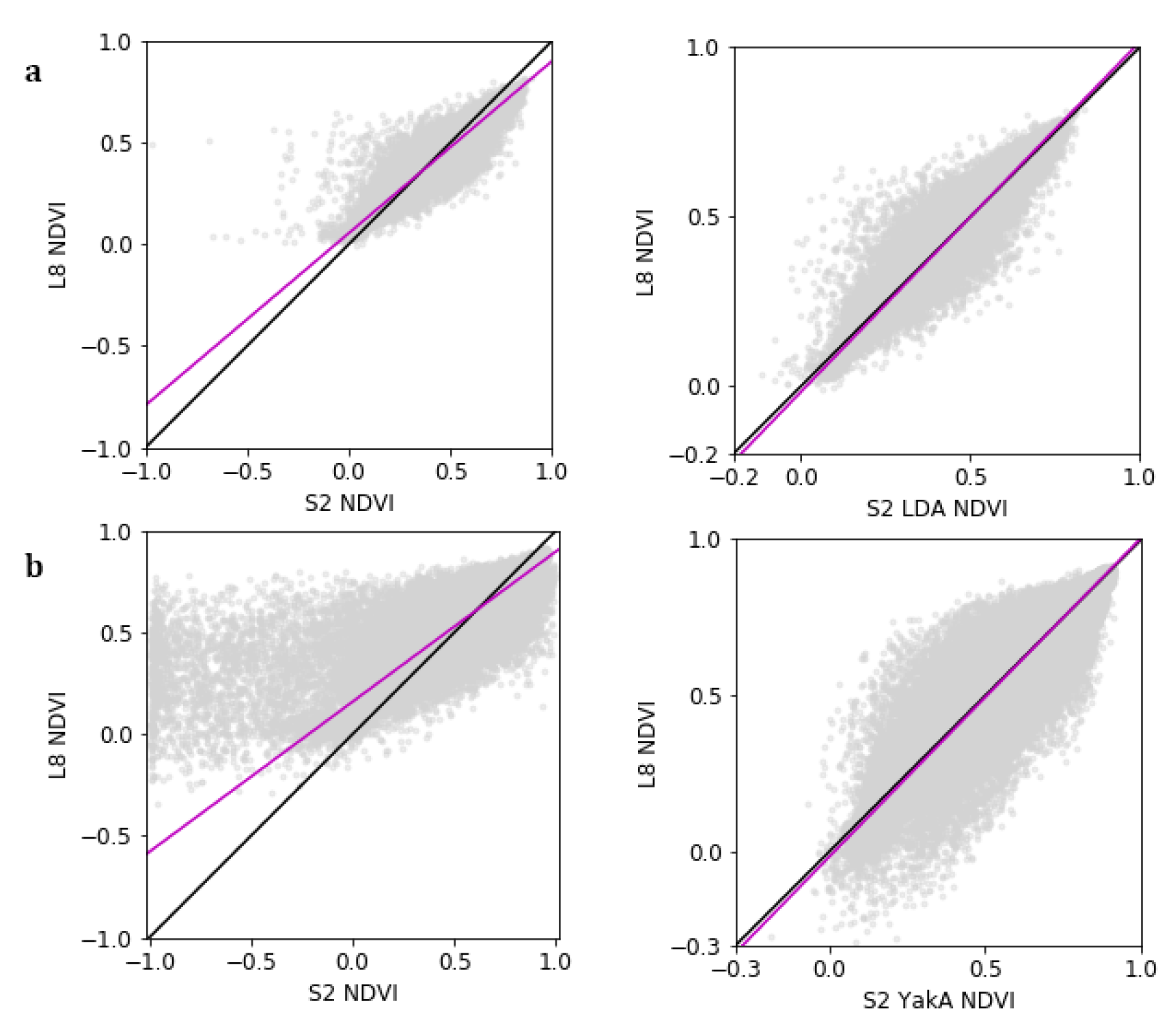
As vegetation indices are extensively used for qualitative and quantitative vegetation cover analyses from spectral measurements, we extended the adjustment assessment to the Normalized Difference Vegetation Index (NDVI). We derived the NDVI, which is commonly used as an indicator of green vegetation cover, for both the Landsat-8 and Sentinel-2 data products. The NDVI is calculated by using two spectral bands, as shown in Equation (2)
where NIR stands for the Near-Infrared wavelength band values and Red for the red wavelength band values of the individual sensor [66]. The NDVI can range between −1 and 1, where an NDVI close to 1 indicates high green vegetation cover and a value close to 0 no vegetation, possibly urban areas, and negative NDVI values mainly result from water, clouds or snow. For the Landsat-8 NDVI calculation, we used B5 for NIR and B4 for red, and for the Sentinel-2 NDVI calculation, we used B8A for NIR and B4 for red (Table 1). We calculated the NDVI for the measured surface reflectance Landsat-8 and Sentinel-2 values and also for the spectrally-adjusted Sentinel-2 reflectance values to assess what effect the spectral differences of Landsat-8 and Sentinel-2 might have on vegetation indices.
3. Results
3.1. Spectral Band Comparison
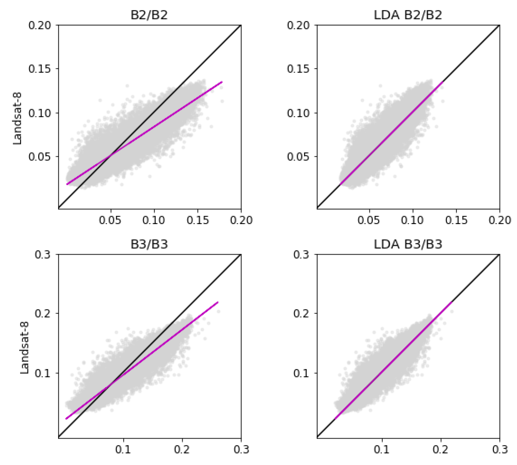
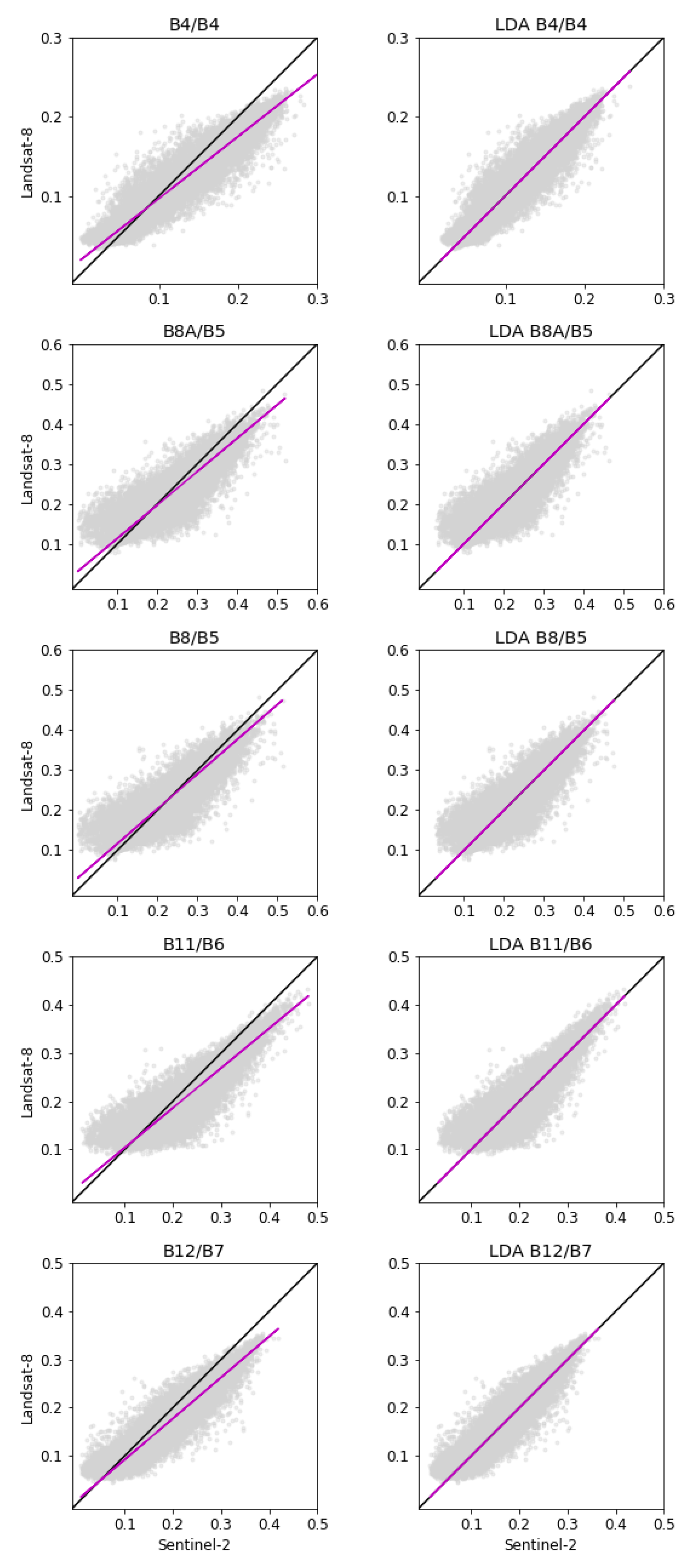
The spectral band comparisons were conducted for all pixels of the overlapping areas from the same-day Sentinel-2 and Landsat-8 acquisitions for every corresponding band combination and for all study sites. Table 3 summarizes the analysis for each study area and provides the intercept and slope of the resulting ordinary least squares regression, Pearson’s correlation coefficients, and associated root mean squared errors. Exemplarily, Figure 4 shows the scatter plots of band combinations and adjusted Sentinel-2 data for the Lena Delta. Figure 4 depicts the expected offset between corresponding bands and scatter around the one-to-one line. In general, the scatter plots affirm that the Landsat-8 and Sentinel-2 bands have a strong overall correlation. This is also represented by high r coefficients and promising ordinary least squares regression coefficients as low intercept and high slope values (Table 3). The comparison scatter plots of Batagay, Yakutsk, and Eastern Siberia are provided in the Appendix (Figure A1, Figure A2 and Figure A3).
The band comparisons of the visible wavelength bands, B2/B2, B3/B3, and B4/B4 for Batagay (Figure A1), showed noticeably lower correlation coefficients, 0.624, 0.726, and 0.818, respectively. The slope coefficients from the ordinary least squares regression were lower for these band combinations in Batagay as well, compared to the other two study sites and the regional ES assessment (Table 3).
We compared both possible NIR band combinations, B8A/B5 and B8/B5, to inspect if one Sentinel-2 NIR band, B8A or B8, was more similar and fits spectrally better to the Landsat-8 NIR band (B5) in combined studies in Eastern Siberia. The results showed no striking trend favoring one band combination. The B8A/B5 comparison overall had slightly higher correlation coefficients than the B8/B5 comparison. Likewise, the RMSE was also smaller for B8A/B5, indicating a closer fit between Sentinel-2 B8A and Landsat-8 B5 reflectance values. The ordinary least squares regression analyses showed contrasting trends, however. The B8A/B5 band comparisons resulted in intercepts that were slightly lower and therefore indicated a marginally better fit. In contrast, the B8/B5 comparison yielded higher slopes, which suggested a regression fit of the two variables.
Overall, the study sites did not differ from one another significantly. The r coefficients ranged between 0.89 (ES B2/B2) and 0.974 (Yakutsk and ES B12/B7), which points at very strong correlations between the Sentinel-2 and Landsat-8 surface reflectance values for all assessed corresponding bands at all study sites. Furthermore, the ordinary least squares regression analyses mainly showed very low intercept and reasonably high slope values.
3.2. Spectral Band Adjustment
The ordinary least squares regression results (Table 3) were used as the input for the spectral band adjustment, using Equation (1). With these coefficients, we adjusted the observed Sentinel-2 surface reflectance values to fit the Landsat-8 values with respect to the band combination and specific study sites. The adjusted Sentinel-2 results are shown exemplarily for the Lena Delta site in Figure 4, while the other two sites, as well as the overall adjustment for Eastern Siberia are shown in the Appendix (Figure A1, Figure A2 and Figure A3).
The overall results showed that the Sentinel-2 surface reflectance values can be fitted to the Landsat-8 pixel surface reflectance values (Table 4). After the spectral band adjustment by band pair, we recalculated the r coefficient, RMSE, and also the new ordinary least squares regression. Visually, the adjusted Sentinel-2 and Landsat-8 surface reflectance values were well aligned with the one-to-one line (Figure 4, Figure A1, Figure A2, and Figure A3). The new intercept and slope results of the ordinary least squares regression now showed that the adjusted datasets had no offset (0) and a slope that was either 0.99 or 1.0, indicating a very good agreement between the two variables. The spread around the mean, demonstrated by the r coefficient, was unchanged, but the RMSE decreased for all band combinations in all study sites. This indicates that the absolute difference between the adjusted Sentinel-2 and Landsat-8 reflectance values for corresponding pixels declined overall. Our results showed that the individual bands correlated better after the Sentinel-2 adjustment for all three study sites and also the Eastern Siberian (ES) regional scale analysis.
The comparison of the NDVI calculations showed one distinct feature. Negative Landsat-8 NDVI values were found only for few pixels, whereas for Sentinel-2 NDVI values before the adjustment, there were considerably more negative values, especially in Yakutsk. However, after spectral band adjustment, there were hardly any remaining negative Sentinel-2 NDVI values. This was valid for all study sites (Figure 5 and Figure A4). Negative NDVI values normally indicate non-vegetated land cover types such as snow, clouds, or water with their higher reflectance properties in the visible wavelengths and then a reflectance decline towards near infrared. Despite this, the NDVI comparisons depicted overall a good fit between Landsat-8 NDVI and Sentinel-2 NDVI values for all study sites, with r coefficients ranging from 0.85 (Batagay) to 0.98 (Lena Delta) (Table 5). The ordinary least squares regression coefficients, as well as the r and RMSE improved with the Sentinel-2 spectral band adjustment when recalculating the Sentinel-2 NDVI with the adjusted NIR and red values (Figure 5 and Table 5).
3.3. ES and HLS Spectral Band Adjustment
We used the ES ordinary least squares regression coefficients (Table 3) as input for Equation (1) and applied these for spectral band adjustment to the three study sites. The results showed that using the ES coefficients for band adjustment also significantly improved the relationship between ES-adjusted Sentinel-2 and Landsat-8 surface reflectance pixel values (Table 6). Visually, there was an improvement and a better relationship between ES-adjusted Sentinel-2 and Landsat-8 reflectance values (Figure A5). The already previously-observed lower correlation of the visible wavelength bands (B2/B2, B3/B3, and B4/B4) in Batagay were noticeable in this assessment as well.
The slope coefficients of the ordinary least squares regression after ES adjustment ranged from 0.928 (Lena Delta B2/B2) to 1.059 (Lena Delta B8/B5). Applying the ES-adjustment coefficients led to some slope coefficients exceeding 1.0 and intercepts that were slightly negative. This was the case for individual band combinations in the Lena Delta and Yakutsk.
Yakutsk seemed to be adjusted the best compared to the Lena Delta and Batagay. This likely was because the ES dataset was dominated by the Yakutsk site, which provided about 80% of the data to the analysis with 1,944,414 pixels compared to 156,315 and 346,053 pixels from the Lena Delta and Batagay sites, respectively (Table 2).
Applying the globally-available HLS coefficients for band adjustment to the three study sites showed no significant improvement (Table 6). The HLS results actually very much resembled the original spectral band comparisons (Table 3). Hence, the relationship between HLS-adjusted Sentinel-2 and Landsat-8 pixel values was not enhanced after HLS adjustment.
4. Discussion
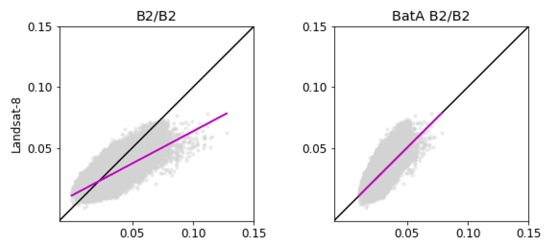
Our overall comparison and adjustment results showed a good fit between Sentinel-2 and Landsat-8 in the high latitudes. Despite this, the Batagay study site showed the biggest differences between Landsat-8 and Sentinel-2 reflectance values in the visible wavelength bands. The Batagay same-day image pair, compared to the Lena Delta and Yakutsk example, also contained the highest cloud cover with 38.6% and 49.8% (Table 2). While the cloud and cloud shadow detection algorithms still had high omission errors [57,64], the Batagay images particularly were visibly contaminated with thin cirrus clouds that were difficult to mask. This decreased the quality of the images [67] and likely was the main cause for a lower correlation coefficient between spectral bands, since the visible wavelength ranges were particularly affected by clouds and cirrus [68]. Landsat-8 and Sentinel-2 were differently sensitive to cirrus clouds, and the acquisition delay of 25 min between the two sensors was sufficient for a change in cirrus conditions in terms of cirrus presence and intensity, which decreased the comparison quality. Claverie et al. [38] observed this in images with a high cloud cover content as well. The geographic location of the Batagay site between two mountain ranges with very frequent cloud cover and highly variable cloud dynamics precludes better same-day image pair qualities. Arguably, the Batagay image pair should therefore be considered with additional caution; however, in spite of the slightly less favorable adjustment fit, the Batagay study site still had good overall adjustment results and illustrated the applicability of this approach also for challenging areas.
All scatter plots had a reasonable amount of scatter around the one-to-one relationship. Experiments with simulated Landsat-8 and Sentinel-2 data by Zhang et al. [33] demonstrated that the scatter was emerging from the differing spectral response functions of the bands. Another source for value scatter likely was the different spatial resolutions of the sensors. Mandanici and Bitelli [34] performed tests that showed that spatially-heterogeneous target surfaces created a lower Pearson correlation coefficient in band comparisons [34]. The Sentinel-2 sensors’ high-resolution bands most likely capture the landscape heterogeneity to a greater extent compared to Landsat-8, which then is not averaged out completely in the resampling process to 60-m pixels. Flood [39] and Roy et al. [69,70] further looked at misregistration, different viewing geometries, and atmospheric path length as potential sources for errors between the sensors. All these points contribute to the scatter between Sentinel-2 and Landsat-8 reflectance values. Overall, we are confident with our adjustment results as the Pearson’s correlation coefficients were high throughout the analyses.
When inspecting the scatter plots, a noticeable number of pixels displayed data discrepancies in the NIR (B8A/B5, B8/B5) and SWIR (B11/B6, B12/B7) band comparisons of Yakutsk and the Lena Delta. In the Lena Delta, Landsat-8 captured little reflectance variability in bands B5 and B6 (between 0.08 and 0.13), while Sentinel-2 recorded reflectance values from 0–0.35 in bands B8A, B8, and B11 for the corresponding pixels. In Yakutsk, the relationship was reversed, where Sentinel-2 recorded nearly no variation in values (0–0.05) in bands B8A, B8, and B11, while Landsat-8 indicated values ranging from 0–0.2 in bands B5 and B6 for the same pixels. This data illustrated the different sensitivities of the two sensors in signal reception and translation to reflectance values. We identified these pixels by building masks to only select the pixels associated with these discrepancies. The majority of these pixels were water or mixed water-land pixels. In the Lena Delta, those pixels were mainly from sandbanks. Despite applying a water mask, these pixels were not masked as they did not fully comply with water characteristics only. The sandbanks have a high bottom reflectance through the thin water column, resulting in mixed reflectance signals, and the extent of water coverage changes strongly with water level changes. Therefore, the water mask failed to mask these pixels properly, and evidently, the Landsat-8 and Sentinel-2 NIR and SWIR bands picked up and converted the mixed signals differently. Likewise, the striking pixels in the Yakutsk NIR and SWIR bands were water body pixels, as well. The Yakutsk area contains many thermokarst lakes and ponds that vary in size and depth, which fosters the likelihood of pixels containing a mixed water and ground signal. Vuolo et al. [35] made similar observations in pixel differences and accredited the bigger differences to three error sources: heterogeneous and complex terrains, the quality of cloud and cloud shadow masking algorithms, and the challenging and differing atmospheric correction results. Our analyses and study site characteristics confirmed these points and challenges, which underlines that a spectral band comparison can only be based on clear, high-quality images, as reflectance artifacts decrease the quality of the comparison and the adjustment scheme results. Further attention has to be given to the cloud, cloud shadow, and water masking. Under challenging conditions, a manual selection and masking of clear areas for analysis may be inevitable. The NDVI comparison results showed that both Landsat-8 and Sentinel-2 NDVI captured similar vegetation traits and that green vegetation estimations derived from either system would be very similar. However, in this case, it was inevitable to adjust the Sentinel-2 bands spectrally to Landsat-8 since a moderate amount of non-adjusted Sentinel-2 NDVI values were negative in contrast to the Landsat-8 NDVI values.
The overall results demonstrated that Sentinel-2- and Landsat-8-acquired reflectance values for corresponding pixels correlated well in Arctic-Boreal permafrost regions in Eastern Siberia. This was observed for all three study sites separately and also in the combined adjustment for the Eastern Siberian region. This underlines the expected sensor compatibility and agrees with results from similar studies [33,34,36,38,39]. However, our study went slightly beyond some of the previous ones, which partly based their evaluation on simulated Landsat-8 and/or Sentinel-2 image products [33,34,36], and not on acquired images. We showed that it is possible to reduce the persistent difference in spectral responses between the measured reflectance values of the spectral bands by deriving and then applying an ordinary least squares regression model, adjusting Sentinel-2 to resemble Landsat-8 reflectance values in Arctic-Boreal permafrost regions. It is possible to create a seemingly perfect fit between spectrally corresponding bands at the individual study site. The best adjustment results were obtained in the local assessments (LDA, BatA, YukA), but closely followed by the regional approach (esA). The ES analysis shows that combining regional data, and deriving overarching adjustment coefficients will lead to a very good fit between Landsat-8 and ES adjusted Sentinel-2 reflectance values in Eastern Siberia as well. We therefore considered our derived adjustment coefficients to be representative for Eastern Siberia and that they were applicable for a Sentinel-2 to Landsat-8 adjustment throughout Eastern Siberia. The implementation of the globally-applicable HLS coefficients did not improve the spectral comparability of Landsat-8 and Sentinel-2 reflectance values at any of our three Arctic-Boreal study sites or on the regional ES level. This might be because only a few Arctic study sites and merely one Siberian site were included in the HLS product, and therefore, the Eastern Siberian landscape and vegetation forms were not represented enough in the HLS study. This finding is similar to the adjustment results from Flood [39] for Australian landscapes, and thus, we do not recommend using globally-derived adjustment coefficients for local or regional scale studies, but instead determine region-specific coefficients for a Sentinel-2 to Landsat-8 adjustment.
Being able to adjust Sentinel-2 to Landsat-8 gives the possibility of combining Landsat and Sentinel-2 data in analysis applications. Here, we relied on the already existing data continuity strategy for the Landsat sensors and would like to extend the range of sensors by adjusting Sentinel-2 to Landsat-8 [29,30,31,32]. Considering the substantial increase in available multispectral images for the high latitudes with Sentinel-2 (Figure 1) [28], the creation of dense time series is possible. A combined Landsat and Sentinel-2 time series will improve land cover and vegetation mapping and monitoring approaches in detecting shifts in vegetation composition and structure, as well as permafrost region disturbances in a warming climate. A key advantage of dense time series analysis is the capability to detect landscape dynamics and to differentiate between rapid and gradual changes, therefore describing permafrost region disturbances better and being able to conduct detailed trend analysis in Arctic-Boreal permafrost regions.
One of the main motivation to combine Landsat-8 and Sentinel-2 in high latitudes is the frequent cloud cover and therefore the low data availability of cloud-free images. To avoid this disadvantage of optical remote sensing altogether, one can consider using Synthetic Aperture Radar (SAR) sensors that penetrate the cloud cover and acquire data during bad weather conditions, as well. SAR data were applied to a variety of studies focusing on different aspects and applications in northern high latitudes, such as land cover mapping, successfully already [20]. Nonetheless, one general conclusion is that the best results can be obtained from polarimetric SAR data together with optical remote sensing [71]. Despite the advantages of active sensors, in particular SAR, towards frequent cloud cover, we trust assessing permafrost landscape changes with optical remote sensing. On the one hand, the optical remote sensing data archive, mainly Landsat, is the longest archive spanning more than 45 years, providing extensive records of the past. On the other hand, we see high potential in change detection and time series segmentation algorithms, such as LandTrendr, which we would like to apply to permafrost regions and assess disturbance regimes. However, the availability and advantages of SAR data will be an asset when assessing permafrost disturbances, as SAR data can potentially fill data gaps and help as supplementary material to identify and evaluate permafrost landscape disturbances well.
5. Conclusions
The overall objective of our study was to compare the spectral characteristics of Landsat-8 and Sentinel-2 across Arctic-Boreal permafrost regions and to assess their compatibility and potential use in a combined time series. Our spectral comparison of Landsat-8 and Sentinel-2 corresponding bands showed that these two sensors correlate well and depict similar trends with only minor differences in Eastern Siberian permafrost regions. Depending on the application purpose, one has to assess whether these differences are negligible or of relevance. With an ordinary least squares regression based on band comparisons of corresponding Landsat-8 and Sentinel-2 bands, we can successfully adjust the Sentinel-2 reflectance values to resemble Landsat-8 more and homogenize the two data sets. To avoid geolocation errors and account for the sensors’ different spatial resolutions, we downscaled our images to 60 m.
The comparison method was valid for adjustments on the local level for sites with different ecological and landscape characteristics, but also when merging data across Eastern Siberia and conducting the spectral comparison and adjustment regionally. This underlines the comparability and compatibility of the two sensors. In contrast, we found that the application of the Harmonized Landsat Sentinel-2 product generated no improvement in spectral adjustment. Relying on global adjustment schemes between Landsat-8 and Sentinel-2 is therefore not advisable for Eastern Siberia or for local to regional time series studies in general. Therefore, we recommend at least regionally-fitted spectral adjustments when jointly using Landsat-8 and Sentinel-2 data products. This minimizes the potentially introduced error from different spectral band responses when combining data from multiple sensors. Our data enable the combined use of Landsat and Sentinel-2 in future time series analysis and other landscape change approaches in Arctic-Boreal permafrost regions of Eastern Siberia. Despite the overall good adjustment results, small differences between the sensors remained, which can be attributed to several factors including heterogeneous terrain, poor cloud and cloud shadow masking, and mixed pixels.
Our assessment was solely based on the use of open source software (GEE, SNAP, Jupyter Notebook) and freely-available data sets (Landsat-8, Sentinel-2). This makes the methodological approach reproducible and allows wide usage also for other study areas. As our results were in line with previous local and regional studies, we acknowledge that these services and softwares are a valuable and useful tool appropriate for such comparison studies.
Author Contributions
A.R. conceptualized the study design, processed, analyzed, and visualized the data, and wrote the original manuscript. G.G. contributed to the study concept and the writing and editing of the manuscript and was responsible for funding acquisition and project administration.
Funding
This research was funded by the BMBF project KoPf (Grant Number 03F0764B), ESA GlobPermafrost, and ERC PETA-CARB (Grant Number 338335).
Acknowledgments
We acknowledge the support of the Deutsche Forschungsgemeinschaft und Open Access Publishing Fund of University of Potsdam. The authors thank Google for providing the GEE platform at no cost, as well as ESA and USGS for providing Sentinel-2 and Landsat-8 satellite imagery at no cost. Furthermore, the authors thank the three reviewers and editors for their time and valuable input to this manuscript.
Conflicts of Interest
The authors declare no conflict of interest.
Abbreviations
The following abbreviations are used in this manuscript:
| BatA | Batagay adjusted |
| ES | Eastern Siberia |
| ESA | European Space Agency |
| esA | Eastern Siberia adjusted |
| GEE | Google Earth Engine |
| HLS | Harmonized Landsat Sentinel-2 Product |
| L8 | Landsat-8 |
| LaSRC | Landsat 8 Surface Reflectance Code |
| NDVI | Normalized Difference Vegetation Index |
| S2 | Sentinel-2 |
| SAR | Synthetic Aperture Radar |
| SNAP | Sentinel Application Platform |
| USGS | United States Geological Survey |
| YakA | Yakutsk Adjusted |
Appendix A

Table A1.
The selected same-day images in Google Earth Engine (GEE) after data filtering for the three study sites.
Table A1.
The selected same-day images in Google Earth Engine (GEE) after data filtering for the three study sites.
| Study Site | Sensor | Image Name GEE |
|---|---|---|
| Lena Delta | L8 | LC08_132009_20160823 |
| S2 | 20160823T034732_20160823T091448_T51XXA | |
| Batagay | L8 | LC08_122012_20160801 |
| S2 | 20160801T030546_20160801T064303_T53WMR | |
| Yakutsk | L8 | LC08_121017_20160709 |
| S2 | 20160709T030011_20160709T081153_T52VEP |
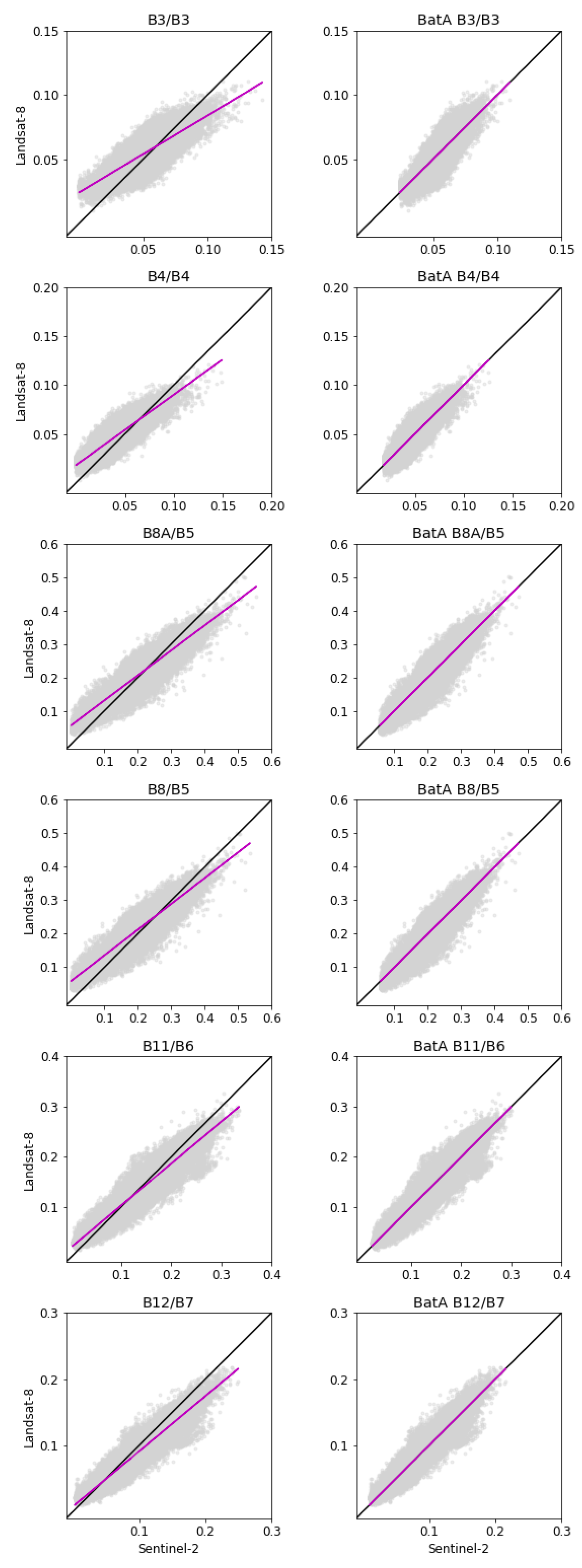
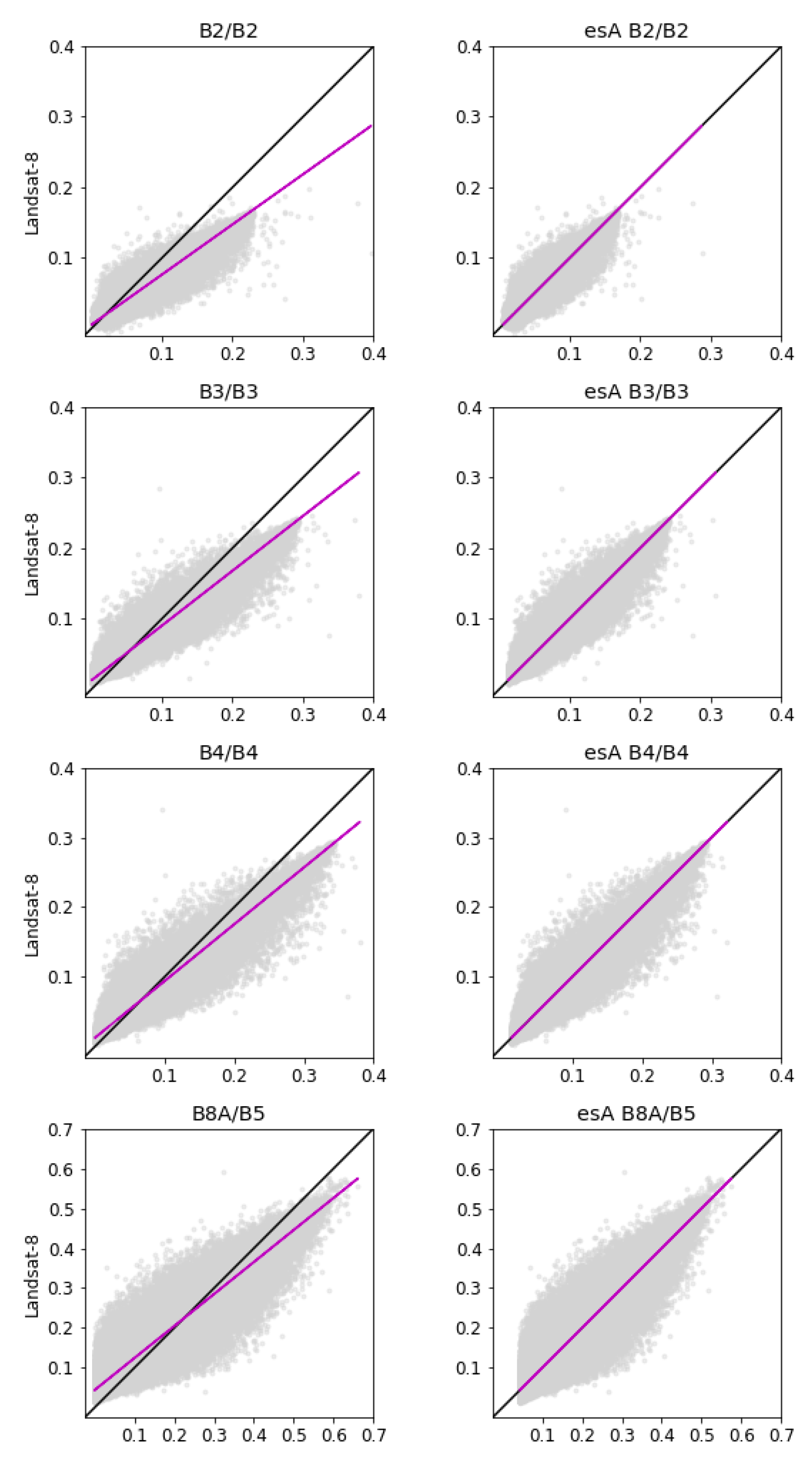
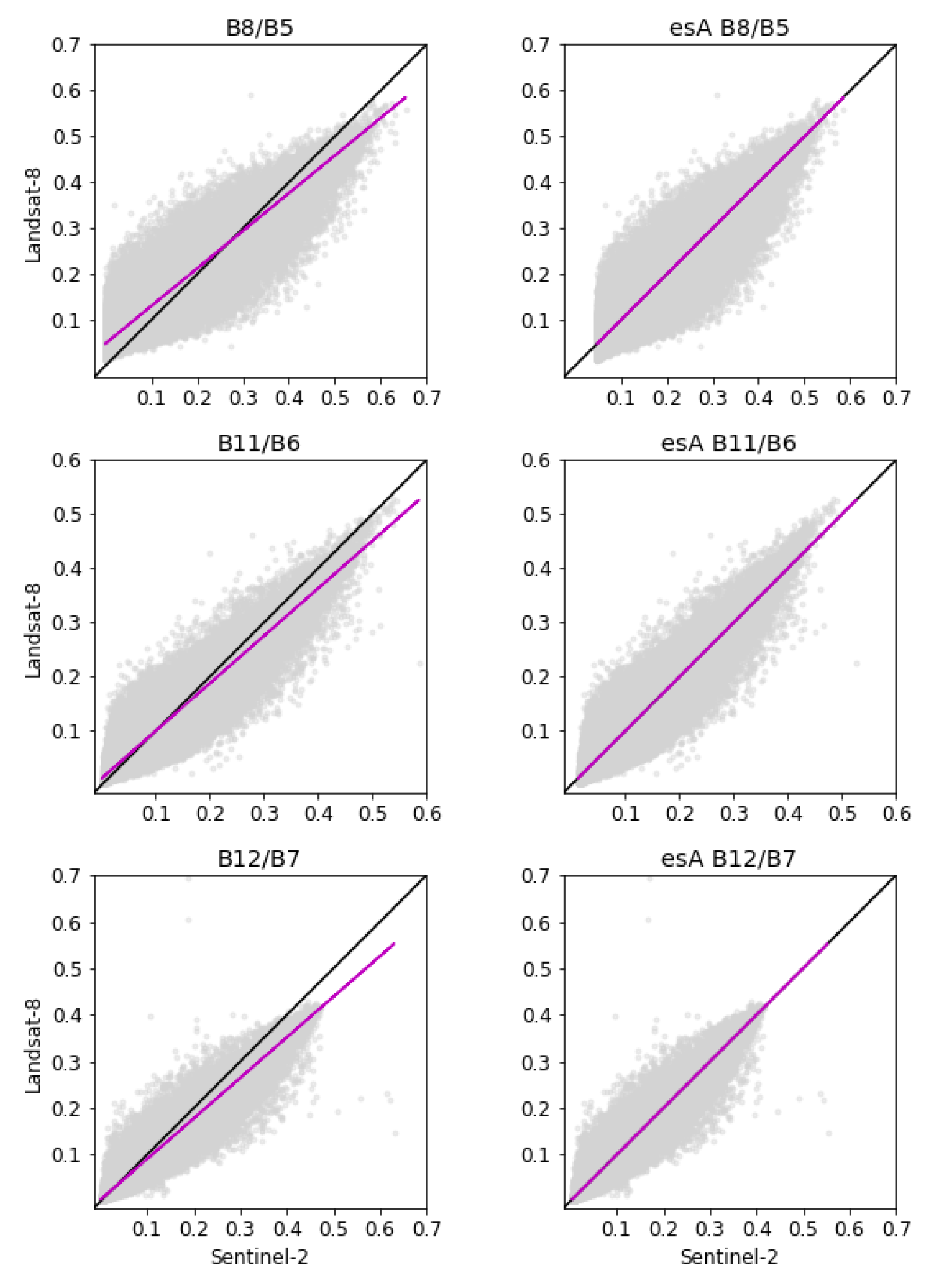
Figure A1.
Comparison of surface reflectance values from the Sentinel-2 and Landsat-8 corresponding bands for Batagay. Left plots: observed surface reflectance values. Right plots: Batagay Adjusted (BatA) Sentinel-2 reflectance values. The solid black line is one-to-one, and the pink line is the ordinary least squares regression trend line.


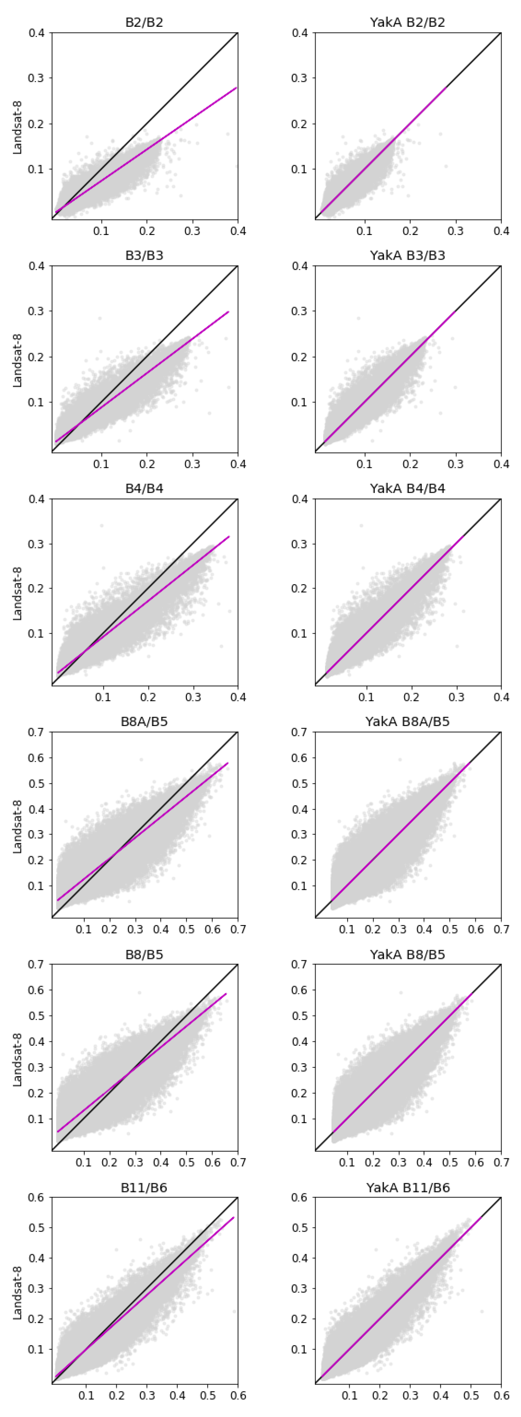
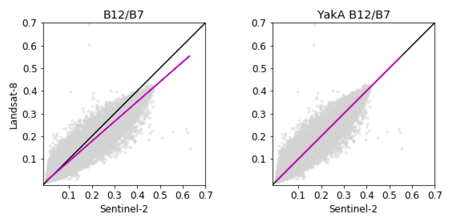
Figure A2.
Comparison of surface reflectance values from the Sentinel-2 and Landsat-8 corresponding bands for Yakutsk. Left plots: observed surface reflectance values. Right plots: Yakutsk Adjusted (YukA) Sentinel-2 reflectance values. The solid black line is one-to-one, and the pink line is the ordinary least squares regression trend line.


Figure A3.
Comparison of surface reflectance values from the Sentinel-2 and Landsat-8 corresponding bands for Eastern Siberia. Left plots: observed surface reflectance values. Right plots: Eastern Siberia Adjusted (esA) Sentinel-2 reflectance values. The solid black line is one-to-one, and the pink line is the ordinary least squares regression trend line.


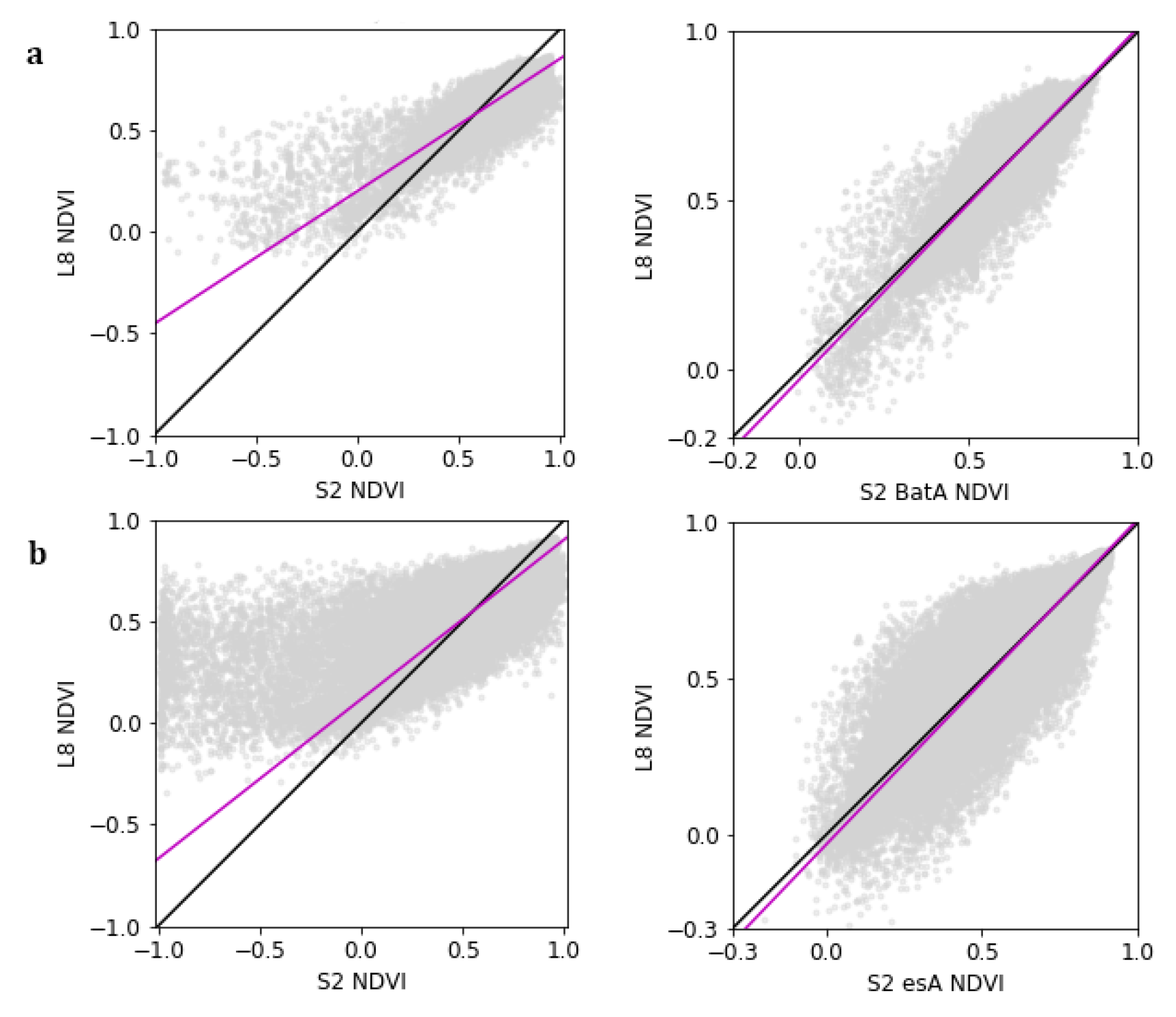
Figure A4.
Comparison of NDVI values from Batagay ((a), upper row) and Eastern Siberia ((b), lower row). Left plots: NDVI calculated from observed surface reflectance values. Right plots: NDVI calculated from adjusted Sentinel-2 reflectance values. The solid black line is one-to-one, and the pink line is the ordinary least squares regression trend line.

Figure A5.
Comparison of Eastern Siberian Adjusted (esA) the Sentinel-2 reflectance values and Landsat-8 corresponding bands for the individual study sites. In the order from left to right: Lena Delta, Batagay, and Yakutsk. The solid black line is one-to-one, and the pink line is the ordinary least squares regression trend line.

References
- Serreze, M.C.; Barry, R.G. Processes and impacts of Arctic amplification: A research synthesis. Glob. Planet. Chang. 2011, 77, 85–96. [Google Scholar] [CrossRef]
- Kaplan, J.O.; New, M. Arctic climate change with a 2 °C global warming: Timing, climate patterns and vegetation change. Clim. Chang. 2006, 79, 213–241. [Google Scholar] [CrossRef]
- Brown, J.; Ferrians, O.; Heginbottom, J.; Melnikov, E. Circum-Arctic Map of Permafrost and Ground-Ice Conditions; Version 2; National Snow and Ice Data Center: Boulder, CO, USA, 2002. [Google Scholar]
- Zhang, T.; Barry, R.; Knowles, K.; Heginbottom, J.; Brown, J. Statistics and characteristics of permafrost and ground-ice distribution in the Northern Hemisphere. Pol. Geogr. 2008, 31, 47–68. [Google Scholar] [CrossRef]
- Schuur, E.A.; Mack, M.C. Ecological response to permafrost thaw and consequences for local and global ecosystem services. Ann. Rev. Ecol. Evol. Syst. 2018, 49, 279–301. [Google Scholar] [CrossRef]
- Biskaborn, B.K.; Smith, S.L.; Noetzli, J.; Matthes, H.; Vieira, G.; Streletskiy, D.A.; Schoeneich, P.; Romanovsky, V.E.; Lewkowicz, A.G.; Abramov, A.; et al. Permafrost is warming at a global scale. Nat. Commun. 2019, 10, 264. [Google Scholar] [CrossRef] [PubMed]
- Chadburn, S.E.; Burke, E.; Cox, P.; Friedlingstein, P.; Hugelius, G.; Westermann, S. An observation-based constraint on permafrost loss as a function of global warming. Nat. Clim. Chang. 2017, 7, 340. [Google Scholar] [CrossRef]
- Francis, J.A.; White, D.M.; Cassano, J.J.; Gutowski, W.J.; Hinzman, L.D.; Holland, M.M.; Steele, M.A.; Vörösmarty, C.J. An arctic hydrologic system in transition: Feedbacks and impacts on terrestrial, marine, and human life. J. Geophys. Res. Biogeosci. 2009, 114, G04019. [Google Scholar] [CrossRef]
- Hicks Pries, C.E.; Van Logtestijn, R.S.; Schuur, E.A.; Natali, S.M.; Cornelissen, J.H.; Aerts, R.; Dorrepaal, E. Decadal warming causes a consistent and persistent shift from heterotrophic to autotrophic respiration in contrasting permafrost ecosystems. Glob. Chang. Biol. 2015, 21, 4508–4519. [Google Scholar] [CrossRef]
- Anthony, K.W.; von Deimling, T.S.; Nitze, I.; Frolking, S.; Emond, A.; Daanen, R.; Anthony, P.; Lindgren, P.; Jones, B.; Grosse, G. 21st-century modeled permafrost carbon emissions accelerated by abrupt thaw beneath lakes. Nat. Commun. 2018, 9, 3262. [Google Scholar] [CrossRef]
- Hjort, J.; Karjalainen, O.; Aalto, J.; Westermann, S.; Romanovsky, V.E.; Nelson, F.E.; Etzelmüller, B.; Luoto, M. Degrading permafrost puts Arctic infrastructure at risk by mid-century. Nat. Commun. 2018, 9, 5147. [Google Scholar] [CrossRef]
- Grosse, G.; Goetz, S.; McGuire, A.D.; Romanovsky, V.E.; Schuur, E.A. Changing permafrost in a warming world and feedbacks to the Earth system. Environ. Res. Lett. 2016, 11, 040201. [Google Scholar] [CrossRef]
- Jorgenson, M.; Grosse, G.; Jones, B.; Arp, C.; Glasser, N.; Cherkauer, K.; Bowling, L.; Naz, B.; Davies, T. 8.20 Thermokarst Terrains; Elsevier: Amsterdam, The Netherlands, 2013. [Google Scholar]
- Romanovsky, V.E.; Smith, S.L.; Christiansen, H.H. Permafrost thermal state in the polar Northern Hemisphere during the international polar year 2007–2009: A synthesis. Permafr. Periglac. Process. 2010, 21, 106–116. [Google Scholar] [CrossRef]
- Woo, M.K.; Kane, D.L.; Carey, S.K.; Yang, D. Progress in permafrost hydrology in the new millennium. Permafr. Periglac. Process. 2008, 19, 237–254. [Google Scholar] [CrossRef]
- Collins, S.; Swinton, S.; Anderson, C.; Gragson, T.; Grimm, N.; Grove, M.; Knapp, A.; Kofinas, G.; Magnuson, J.; McDowell, B.; et al. Integrated science for society and the environment: A strategic research initiative. Albuquerque, Long-Term Ecological Research Network, Publication. 2007. Available online: https://lternet.edu/ (accessed on 5 July 2019).
- Grosse, G.; Harden, J.; Turetsky, M.; McGuire, A.D.; Camill, P.; Tarnocai, C.; Frolking, S.; Schuur, E.A.; Jorgenson, T.; Marchenko, S.; et al. Vulnerability of high-latitude soil organic carbon in North America to disturbance. J. Geophys. Res. Biogeosci. 2011, 116. [Google Scholar] [CrossRef] [Green Version]
- Jorgenson, M.T.; Grosse, G. Remote sensing of landscape change in permafrost regions. Permafr. Periglac. Process. 2016, 27, 324–338. [Google Scholar] [CrossRef]
- Stow, D.A.; Hope, A.; McGuire, D.; Verbyla, D.; Gamon, J.; Huemmrich, F.; Houston, S.; Racine, C.; Sturm, M.; Tape, K.; et al. Remote sensing of vegetation and land-cover change in Arctic Tundra Ecosystems. Remote Sens. Environ. 2004, 89, 281–308. [Google Scholar] [CrossRef] [Green Version]
- Bartsch, A.; Höfler, A.; Kroisleitner, C.; Trofaier, A. Land cover mapping in northern high latitude permafrost regions with satellite data: Achievements and remaining challenges. Remote Sens. 2016, 8, 979. [Google Scholar] [CrossRef]
- Nitze, I.; Grosse, G.; Jones, B.M.; Romanovsky, V.E.; Boike, J. Remote sensing quantifies widespread abundance of permafrost region disturbances across the Arctic and Subarctic. Nat. Commun. 2018, 9, 5423. [Google Scholar] [CrossRef]
- Pastick, N.J.; Jorgenson, M.T.; Goetz, S.J.; Jones, B.M.; Wylie, B.K.; Minsley, B.J.; Genet, H.; Knight, J.F.; Swanson, D.K.; Jorgenson, J.C. Spatiotemporal remote sensing of ecosystem change and causation across Alaska. Glob. Chang. Biol. 2019, 25, 1171–1189. [Google Scholar] [CrossRef]
- Kennedy, R.E.; Yang, Z.; Cohen, W.B. Detecting trends in forest disturbance and recovery using yearly Landsat time series: 1. LandTrendr—Temporal segmentation algorithms. Remote Sens. Environ. 2010, 114, 2897–2910. [Google Scholar] [CrossRef]
- Sulla-Menashe, D.; Woodcock, C.E.; Friedl, M.A. Canadian boreal forest greening and browning trends: An analysis of biogeographic patterns and the relative roles of disturbance versus climate drivers. Environ. Res. Lett. 2018, 13, 014007. [Google Scholar] [CrossRef]
- USGS. Landsat 8 (L8) Data Users Handbook; USGS: Reston, VA, USA, 2015; Volume 1.
- Hope, A.; Stow, D. Shortwave reflectance properties of arctic tundra landscapes. In Landscape Function and Disturbance in Arctic Tundra; Springer: Berlin/Heidelberg, Germany, 1996; pp. 155–164. [Google Scholar]
- Drusch, M.; Del Bello, U.; Carlier, S.; Colin, O.; Fernandez, V.; Gascon, F.; Hoersch, B.; Isola, C.; Laberinti, P.; Martimort, P.; et al. Sentinel-2: ESA’s optical high-resolution mission for GMES operational services. Remote Sens. Environ. 2012, 120, 25–36. [Google Scholar] [CrossRef]
- Li, J.; Roy, D. A global analysis of Sentinel-2A, Sentinel-2B and Landsat-8 data revisit intervals and implications for terrestrial monitoring. Remote Sens. 2017, 9, 902. [Google Scholar] [CrossRef]
- Flood, N. Continuity of reflectance data between Landsat-7 ETM+ and Landsat-8 OLI, for both top-of-atmosphere and surface reflectance: A study in the Australian landscape. Remote Sens. 2014, 6, 7952–7970. [Google Scholar] [CrossRef]
- Mishra, N.; Haque, M.; Leigh, L.; Aaron, D.; Helder, D.; Markham, B. Radiometric cross calibration of Landsat 8 operational land imager (OLI) and Landsat 7 enhanced thematic mapper plus (ETM+). Remote Sens. 2014, 6, 12619–12638. [Google Scholar] [CrossRef]
- Teillet, P.; Barker, J.; Markham, B.; Irish, R.; Fedosejevs, G.; Storey, J. Radiometric cross-calibration of the Landsat-7 ETM+ and Landsat-5 TM sensors based on tandem datasets. Remote Sens. Environ. 2001, 78, 39–54. [Google Scholar] [CrossRef]
- Teillet, P.; Markham, B.; Irish, R.R. Landsat cross-calibration based on near simultaneous imaging of common ground targets. Remote Sens. Environ. 2006, 102, 264–270. [Google Scholar] [CrossRef] [Green Version]
- Zhang, H.K.; Roy, D.P.; Yan, L.; Li, Z.; Huang, H.; Vermote, E.; Skakun, S.; Roger, J.C. Characterization of Sentinel-2A and Landsat-8 top of atmosphere, surface, and nadir BRDF adjusted reflectance and NDVI differences. Remote Sens. Environ. 2018, 215, 482–494. [Google Scholar] [CrossRef]
- Mandanici, E.; Bitelli, G. Preliminary comparison of sentinel-2 and landsat 8 imagery for a combined use. Remote Sens. 2016, 8, 1014. [Google Scholar] [CrossRef]
- Vuolo, F.; Żółtak, M.; Pipitone, C.; Zappa, L.; Wenng, H.; Immitzer, M.; Weiss, M.; Baret, F.; Atzberger, C. Data service platform for Sentinel-2 surface reflectance and value-added products: System use and examples. Remote Sens. 2016, 8, 938. [Google Scholar] [CrossRef]
- Gorroño, J.; Banks, A.C.; Fox, N.P.; Underwood, C. Radiometric inter-sensor cross-calibration uncertainty using a traceable high accuracy reference hyperspectral imager. ISPRS J. Photogramm. Remote Sens. 2017, 130, 393–417. [Google Scholar] [CrossRef] [Green Version]
- Li, S.; Ganguly, S.; Dungan, J.L.; Wang, W.; Nemani, R.R. Sentinel-2 MSI radiometric characterization and cross-calibration with Landsat-8 OLI. Adv. Remote Sens. 2017, 6, 147. [Google Scholar] [CrossRef]
- Claverie, M.; Ju, J.; Masek, J.G.; Dungan, J.L.; Vermote, E.F.; Roger, J.C.; Skakun, S.V.; Justice, C. The Harmonized Landsat and Sentinel-2 surface reflectance dataset. Remote Sens. Environ. 2018, 219, 145–161. [Google Scholar] [CrossRef]
- Flood, N. Comparing Sentinel-2A and Landsat 7 and 8 using surface reflectance over Australia. Remote Sens. 2017, 9, 659. [Google Scholar] [CrossRef]
- Schneider, J.; Grosse, G.; Wagner, D. Land cover classification of tundra environments in the Arctic Lena Delta based on Landsat 7 ETM+ data and its application for upscaling of methane emissions. Remote Sens. Environ. 2009, 113, 380–391. [Google Scholar] [CrossRef] [Green Version]
- Boike, J.; Kattenstroth, B.; Abramova, E.; Bornemann, N.; Chetverova, A.; Fedorova, I.; Fröb, K.; Grigoriev, M.; Grüber, M.; Kutzbach, L.; et al. Baseline characteristics of climate, permafrost and land cover from a new permafrost observatory in the Lena River Delta, Siberia (1998–2011). Biogeosciences 2013, 10, 2105–2128. [Google Scholar] [CrossRef]
- Morgenstern, A.; Grosse, G.; Günther, F.; Fedorova, I.; Schirrmeister, L. Spatial analyzes of thermokarst lakes and basins in Yedoma landscapes of the Lena Delta. Cryosphere Discuss. 2011, 5, 1495–1545. [Google Scholar] [CrossRef]
- Strauss, J.; Schirrmeister, L.; Grosse, G.; Fortier, D.; Hugelius, G.; Knoblauch, C.; Romanovsky, V.; Schädel, C.; von Deimling, T.S.; Schuur, E.A.; et al. Deep Yedoma permafrost: A synthesis of depositional characteristics and carbon vulnerability. Earth-Sci. Rev. 2017, 172, 75–86. [Google Scholar] [CrossRef] [Green Version]
- Ashastina, K.; Schirrmeister, L.; Fuchs, M.; Kienast, F. Palaeoclimate characteristics in interior Siberia of MIS 6–2: First insights from the Batagay permafrost mega-thaw slump in the Yana Highlands. Clim. Past 2017, 13, 795–818. [Google Scholar] [CrossRef]
- Lydolph, P.E.; Temple, D.; Temple, D. The Climate of the Earth; Government Institutes, 1985. [Google Scholar]
- Ivanova, R. Seasonal thawing of soils in the Yana River valley, northern Yakutia. In Proceedings of the Eighth International Conference on Permafrost, Zürich, Switzerland, 21–25 July 2003; pp. 21–25. [Google Scholar]
- Kunitsky, V.; Syromyatnikov, I.; Schirrmeister, L.; Skachov, Y.B.; Grosse, G.; Wetterich, S.; Grigoriev, M. Ice-rich permafrost and thermal denudation in the Batagay area (Yana Upland, East Siberia). Earth Cryosphere 2013, 17, 56–58. [Google Scholar]
- Günther, F.; Grosse, G.; Jones, B.M.; Schirrmeister, L.; Romanovsky, V.E.; Kunitsky, V. Unprecedented permafrost thaw dynamics on a decadal time scale: Batagay mega thaw slump development, Yana Uplands, Yakutia, Russia. In AGU Fall Meeting Abstracts; American Geophysical Union: Washington, DC, USA, 2016. [Google Scholar]
- Opel, T.; Murton, J.B.; Wetterich, S.; Meyer, H.; Ashastina, K.; Günther, F.; Grotheer, H.; Mollenhauer, G.; Danilov, P.P.; Boeskorov, V.; et al. Middle and Late Pleistocene climate and continentality inferred from ice wedges at Batagay megaslump in the Northern Hemisphere’s most continental region, Yana Highlands, interior Yakutia. Clim. Past Discuss. 2018, 2018, 1–32. [Google Scholar] [CrossRef]
- Fedorov, A.; Gavriliev, P.; Konstantinov, P.; Hiyama, T.; Iijima, Y.; Iwahana, G. Estimating the water balance of a thermokarst lake in the middle of the Lena River basin, eastern Siberia. Ecohydrology 2014, 7, 188–196. [Google Scholar] [CrossRef]
- Fedorov, A.N.; Iwahana, G.; Konstantinov, P.Y.; Machimura, T.; Argunov, R.N.; Efremov, P.V.; Lopez, L.M.; Takakai, F. Variability of permafrost and landscape conditions following clear cutting of larch forest in central Yakutia. Permafr. Periglac. Process. 2017, 28, 331–338. [Google Scholar] [CrossRef]
- Ulrich, M.; Matthes, H.; Schirrmeister, L.; Schütze, J.; Park, H.; Iijima, Y.; Fedorov, A.N. Differences in behavior and distribution of permafrost-related lakes in C entral Y akutia and their response to climatic drivers. Water Resour. Res. 2017, 53, 1167–1188. [Google Scholar] [CrossRef]
- Boike, J.; Grau, T.; Heim, B.; Günther, F.; Langer, M.; Muster, S.; Gouttevin, I.; Lange, S. Satellite-derived changes in the permafrost landscape of central Yakutia, 2000–2011: Wetting, drying, and fires. Glob. Planet. Chang. 2016, 139, 116–127. [Google Scholar] [CrossRef]
- ESA. Sentinel-2 User Handbook; ESA, 2015; Volume 1. Available online: https://sentinel.esa.int/web/sentinel/user-guides/document-library (accessed on 13 March 2018).
- Gorelick, N.; Hancher, M.; Dixon, M.; Ilyushchenko, S.; Thau, D.; Moore, R. Google Earth Engine: Planetary-scale geospatial analysis for everyone. Remote Sens. Environ. 2017, 202, 18–27. [Google Scholar] [CrossRef]
- USGS. Landsat Processing Details. 2018. Available online: https://landsat.usgs.gov/landsat-processing-details (accessed on 5 March 2018).
- Foga, S.; Scaramuzza, P.L.; Guo, S.; Zhu, Z.; Dilley, R.D., Jr.; Beckmann, T.; Schmidt, G.L.; Dwyer, J.L.; Hughes, M.J.; Laue, B. Cloud detection algorithm comparison and validation for operational Landsat data products. Remote Sens. Environ. 2017, 194, 379–390. [Google Scholar] [CrossRef] [Green Version]
- Louis, J.; Debaecker, V.; Pflug, B.; Main-Knorn, M.; Bieniarz, J.; Mueller-Wilm, U.; Cadau, E.; Gascon, F. Sentinel-2 Sen2Cor: L2A processor for users. In Proceedings of the Living Planet Symposium, Prague, Czech Republic, 9–13 May 2016; pp. 9–13. [Google Scholar]
- Müller-Wilm, U.; Devignot, O.; Pessiot, L. Sen2Cor Configuration and User Manual; Telespazio VEGA Deutschland GmbH: Darmstadt, Germany, 2016. [Google Scholar]
- Donchyts, G. Implementation of Basic Cloud Shadow Shift. In Google Earth Engine Code; An Optional Note; Google: Menlo Park, CA, USA, 2017. [Google Scholar]
- Korhonen, L.; Packalen, P.; Rautiainen, M. Comparison of Sentinel-2 and Landsat 8 in the estimation of boreal forest canopy cover and leaf area index. Remote Sens. Environ. 2017, 195, 259–274. [Google Scholar] [CrossRef]
- Storey, J.; Choate, M.; Lee, K. Landsat 8 Operational Land Imager on-orbit geometric calibration and performance. Remote Sens. 2014, 6, 11127–11152. [Google Scholar] [CrossRef]
- Storey, J.; Roy, D.P.; Masek, J.; Gascon, F.; Dwyer, J.; Choate, M. A note on the temporary misregistration of Landsat-8 Operational Land Imager (OLI) and Sentinel-2 Multi Spectral Instrument (MSI) imagery. Remote Sens. Environ. 2016, 186, 121–122. [Google Scholar] [CrossRef] [Green Version]
- Zhu, Z.; Wang, S.; Woodcock, C.E. Improvement and expansion of the Fmask algorithm: Cloud, cloud shadow, and snow detection for Landsats 4–7, 8, and Sentinel 2 images. Remote Sens. Environ. 2015, 159, 269–277. [Google Scholar] [CrossRef]
- Cowan, G. Statistical Data Analysis; Oxford University Press: Oxford, UK, 1998. [Google Scholar]
- Bannari, A.; Morin, D.; Bonn, F.; Huete, A. A review of vegetation indices. Remote Sens. Rev. 1995, 13, 95–120. [Google Scholar] [CrossRef]
- Gómez-Chova, L.; Camps-Valls, G.; Calpe-Maravilla, J.; Guanter, L.; Moreno, J. Cloud-screening algorithm for ENVISAT/MERIS multispectral images. IEEE Trans. Geosci. Remote Sens. 2007, 45, 4105–4118. [Google Scholar] [CrossRef]
- Bartlett, J.S.; Ciotti, Á.M.; Davis, R.F.; Cullen, J.J. The spectral effects of clouds on solar irradiance. J. Geophys. Res. Oceans 1998, 103, 31017–31031. [Google Scholar] [CrossRef]
- Roy, D.P.; Li, J.; Zhang, H.K.; Yan, L.; Huang, H.; Li, Z. Examination of Sentinel-2A multi-spectral instrument (MSI) reflectance anisotropy and the suitability of a general method to normalize MSI reflectance to nadir BRDF adjusted reflectance. Remote Sens. Environ. 2017, 199, 25–38. [Google Scholar] [CrossRef]
- Roy, D.; Li, Z.; Zhang, H. Adjustment of Sentinel-2 multi-spectral instrument (MSI) Red-Edge band reflectance to Nadir BRDF adjusted reflectance (NBAR) and quantification of red-edge band BRDF effects. Remote Sens. 2017, 9, 1325. [Google Scholar] [CrossRef]
- Ullmann, T.; Schmitt, A.; Roth, A.; Duffe, J.; Dech, S.; Hubberten, H.W.; Baumhauer, R. Land cover characterization and classification of arctic tundra environments by means of polarized synthetic aperture X-and C-Band Radar (PolSAR) and Landsat 8 multispectral imagery—Richards Island, Canada. Remote Sens. 2014, 6, 8565–8593. [Google Scholar] [CrossRef]
Figure 1.
Average number of clear pixels for the study site Lena Delta for the summer periods covering 1999–2018 (blue bars: Landsat; red bars: Sentinel-2).
Figure 1.
Average number of clear pixels for the study site Lena Delta for the summer periods covering 1999–2018 (blue bars: Landsat; red bars: Sentinel-2).

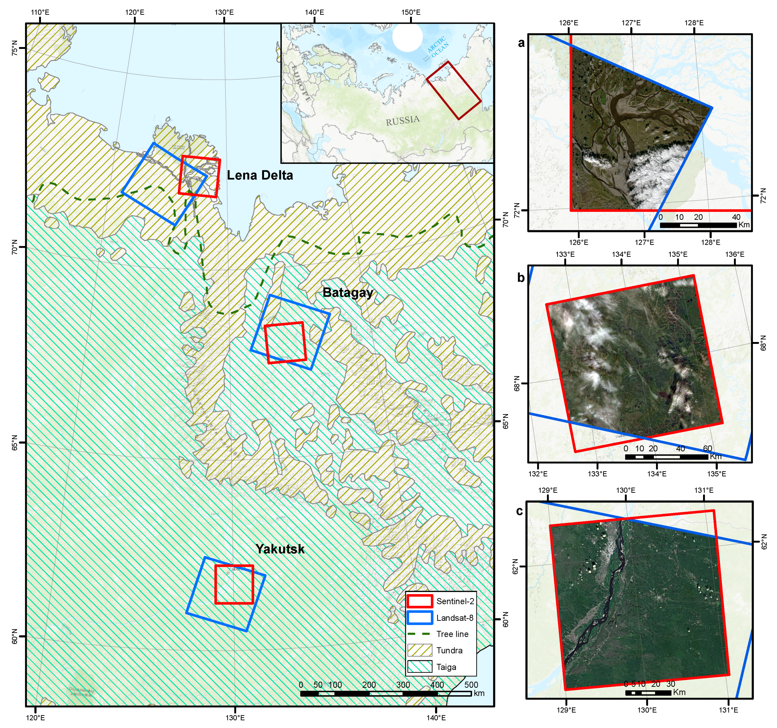
Figure 2.
The three Arctic-to-Boreal study sites, Lena Delta, Batagay region, and Yakutsk region, are located along an approximate north-south transect in Eastern Siberia. The blue frames show the Landsat-8 image footprint, and the red frames show the Sentinel-2 image footprint of the same-day acquisitions used in this study. Sentinel-2 RGB composites of the overlapping area for the Lena Delta (a), Batagay region (b), and Yakutsk region (c).

Figure 3.
Data processing workflow used for the spectral band comparison and adjustment. Landsat-8 is abbreviated to L8 and Sentinel-2 to S2.
Figure 3.
Data processing workflow used for the spectral band comparison and adjustment. Landsat-8 is abbreviated to L8 and Sentinel-2 to S2.

Figure 4.
Comparison of surface reflectance values from the Sentinel-2 and Landsat-8 corresponding bands for the Lena Delta. Left plots: observed surface reflectance values. Right plots: Lena Delta Adjusted (LDA) Sentinel-2 reflectance values. The solid black line is one-to-one, and the pink line is the ordinary least squares regression trend line. In all plots, the Sentinel-2 values and bands are on the x-axis, while Landsat-8 is depicted on the y-axis.


Figure 5.
Comparison of NDVI values from the Lena Delta ((a), upper row) and Yakutsk ((b), lower row). Left plots: NDVI calculated from observed Landsat-8 and Sentinel-2 surface reflectance values. Right plots: NDVI calculated from adjusted Sentinel-2 and observed Landsat-8 reflectance values. The solid black line is one-to-one, and the pink line is the ordinary least squares regression trend line.

Table 1.
Corresponding Landsat-8 and Sentinel-2 bands and characteristics.
| Landsat-8 | Sentinel-2 | |||||
|---|---|---|---|---|---|---|
| Band | Wavelength (μm) | Resolution (m) | Band | Wavelength (μm) | Resolution (m) | |
| Coastal Aerosol | 1 | 0.45–0.451 | 30 | 1 | 0.430–0.450 | 60 |
| Blue | 2 | 0.452–0.51 | 30 | 2 | 0.448–0.546 | 10 |
| Green | 3 | 0.533–0.590 | 30 | 3 | 0.538–0.583 | 10 |
| Red | 4 | 0.636–0.673 | 30 | 4 | 0.646–0.684 | 10 |
| NIR | 5 | 0.851–0.879 | 30 | 8A | 0.848–0.881 | 20 |
| NIR2 | 8 | 0.763–0.908 | 10 | |||
| SWIR1 | 6 | 1.566–1.651 | 30 | 11 | 1.542–1.685 | 20 |
| SWIR2 | 7 | 2.107–2.294 | 30 | 12 | 2.081–2.323 | 20 |
| Cirrus | 9 | 1.363–1.384 | 30 | 10 | 1.336–1.441 | 60 |
Table 2.
Data filtering and selection result for same-day Landsat-8 and Sentinel-2 image pairs for the three study sites.
Table 2.
Data filtering and selection result for same-day Landsat-8 and Sentinel-2 image pairs for the three study sites.
| Location | Date 2016 | Sensor | Cloud Cover % | Acquisition Time (UTC) | Solar Azimuth Angle | Solar Zenith Angle | No. of Clear Pixels | |
|---|---|---|---|---|---|---|---|---|
| Lena Delta | 72.37 N | 23 August | L8 | 24 | 03:40:06 | 178.97 | 60.89 | 156,315 |
| 126.50 E | S2 | 18.5 | 03:47:34 | 184.34 | 61.18 | |||
| Batagay | 67.77 N | 1 August | L8 | 38.6 | 02:39:23 | 170.97 | 50:57 | 346,053 |
| 134.58 E | S2 | 49.8 | 03:05:46 | 179.39 | 50.10 | |||
| Yakutsk | 61.77 N | 9 July | L8 | 1.3 | 02:35:06 | 161.32 | 40.17 | 1,944,414 |
| 130.50 E | S2 | 0.1 | 03:00:11 | 171.07 | 39.65 |
Table 3.
Comparison of surface reflectance values from the Sentinel-2 and Landsat-8 corresponding bands, for same-day acquisitions. Displaying the results of the ordinary least squares regression, Pearson correlation, and root mean squared error for every study site.
Table 3.
Comparison of surface reflectance values from the Sentinel-2 and Landsat-8 corresponding bands, for same-day acquisitions. Displaying the results of the ordinary least squares regression, Pearson correlation, and root mean squared error for every study site.
| Bands | Study | Ordinary Least Squares Regression | Pearson’s Correlation | Root Mean Square | ||
|---|---|---|---|---|---|---|
| S2 Band | L8 Band | Site | Intercept | Slope | Coefficient (r) | Error (RMSE) |
| 2 | 2 | Lena Delta | 0.017 | 0.66 | 0.927 | 0.012 |
| Batagay | 0.0107 | 0.531 | 0.624 | 0.008 | ||
| Yakutsk | 0.0052 | 0.689 | 0.92 | 0.007 | ||
| ES | 0.0053 | 0.711 | 0.89 | 0.0073 | ||
| 3 | 3 | Lena Delta | 0.0186 | 0.767 | 0.962 | 0.0096 |
| Batagay | 0.0240 | 0.599 | 0.726 | 0.008 | ||
| Yakutsk | 0.0129 | 0.752 | 0.945 | 0.006 | ||
| ES | 0.0125 | 0.777 | 0.937 | 0.0065 | ||
| 4 | 4 | Lena Delta | 0.0182 | 0.784 | 0.97 | 0.0104 |
| Batagay | 0.018 | 0.721 | 0.818 | 0.011 | ||
| Yakutsk | 0.012 | 0.8 | 0.964 | 0.009 | ||
| ES | 0.0125 | 0.815 | 0.97 | 0.0095 | ||
| 8A | 5 | Lena Delta | 0.0302 | 0.835 | 0.95 | 0.021 |
| Batagay | 0.056 | 0.749 | 0.902 | 0.019 | ||
| Yakutsk | 0.044 | 0.806 | 0.945 | 0.018 | ||
| ES | 0.044 | 0.804 | 0.941 | 0.019 | ||
| 8 | 5 | Lena Delta | 0.030 | 0.869 | 0.943 | 0.0187 |
| Batagay | 0.058 | 0.771 | 0.900 | 0.020 | ||
| Yakutsk | 0.049 | 0.82 | 0.942 | 0.0201 | ||
| ES | 0.049 | 0.82 | 0.94 | 0.020 | ||
| 11 | 6 | Lena Delta | 0.021 | 0.826 | 0.951 | 0.0241 |
| Batagay | 0.0194 | 0.836 | 0.933 | 0.015 | ||
| Yakutsk | 0.0095 | 0.894 | 0.967 | 0.014 | ||
| ES | 0.012 | 0.877 | 0.97 | 0.015 | ||
| 12 | 7 | Lena Delta | 0.007 | 0.852 | 0.962 | 0.019 |
| Batagay | 0.0077 | 0.834 | 0.938 | 0.0111 | ||
| Yakutsk | 0.0031 | 0.874 | 0.974 | 0.012 | ||
| ES | 0.004 | 0.87 | 0.974 | 0.013 | ||
Table 4.
Comparison of surface reflectance values from the Sentinel-2 and Landsat-8 corresponding bands after spectral band adjustment, for same-day acquisitions. Displaying the results of the ordinary least squares regression, Pearson correlation, and root mean squared error for every study site.
Table 4.
Comparison of surface reflectance values from the Sentinel-2 and Landsat-8 corresponding bands after spectral band adjustment, for same-day acquisitions. Displaying the results of the ordinary least squares regression, Pearson correlation, and root mean squared error for every study site.
| Bands | Study | Ordinary Least Square Regression | Pearson’s Correlation | Root Mean Square | ||
|---|---|---|---|---|---|---|
| S2 Band | L8 Band | Site | Intercept | Slope | Coefficient (r) | Error (RMSE) |
| 2 | 2 | Lena Delta | 0 | 0.99 | 0.927 | 0.007 |
| Batagay | 0 | 1.00 | 0.624 | 0.006 | ||
| Yakutsk | 0 | 0.99 | 0.92 | 0.004 | ||
| ES | 0 | 1.00 | 0.89 | 0.005 | ||
| 3 | 3 | Lena Delta | 0 | 0.99 | 0.962 | 0.006 |
| Batagay | 0 | 1.00 | 0.726 | 0.006 | ||
| Yakutsk | 0 | 1.00 | 0.945 | 0.0042 | ||
| ES | 0 | 1.00 | 0.937 | 0.005 | ||
| 4 | 4 | Lena Delta | 0 | 0.99 | 0.97 | 0.007 |
| Batagay | 0 | 0.99 | 0.818 | 0.006 | ||
| Yakutsk | 0 | 0.99 | 0.964 | 0.0048 | ||
| ES | 0 | 1.00 | 0.97 | 0.0054 | ||
| 8A | 5 | Lena Delta | 0 | 1.00 | 0.95 | 0.016 |
| Batagay | 0 | 0.99 | 0.902 | 0.0153 | ||
| Yakutsk | 0 | 0.99 | 0.945 | 0.0152 | ||
| ES | 0 | 1.00 | 0.941 | 0.0154 | ||
| 8 | 5 | Lena Delta | 0 | 1.00 | 0.943 | 0.017 |
| Batagay | 0 | 0.99 | 0.900 | 0.0154 | ||
| Yakutsk | 0 | 0.99 | 0.942 | 0.0155 | ||
| ES | 0 | 0.99 | 0.94 | 0.0158 | ||
| 11 | 6 | Lena Delta | 0 | 0.99 | 0.951 | 0.013 |
| Batagay | 0 | 1.00 | 0.933 | 0.0112 | ||
| Yakutsk | 0 | 1.00 | 0.967 | 0.0102 | ||
| ES | 0 | 1.00 | 0.97 | 0.0106 | ||
| 12 | 7 | Lena Delta | 0 | 0.99 | 0.962 | 0.011 |
| Batagay | 0 | 1.00 | 0.938 | 0.0075 | ||
| Yakutsk | 0 | 0.99 | 0.974 | 0.0074 | ||
| ES | 0 | 0.99 | 0.974 | 0.0077 | ||
Table 5.
Comparison of NDVI calculations from Sentinel-2 and Landsat-8 before and after spectral band adjustment (NDVI adj), for same-day acquisitions. Displaying the results of the ordinary least squares regression, Pearson correlation, and root mean squared error for every study site.
Table 5.
Comparison of NDVI calculations from Sentinel-2 and Landsat-8 before and after spectral band adjustment (NDVI adj), for same-day acquisitions. Displaying the results of the ordinary least squares regression, Pearson correlation, and root mean squared error for every study site.
| Bands | Study | Ordinary Least Square Regression | Pearson’s Correlation | Root Mean Square | ||
|---|---|---|---|---|---|---|
| S2 Band | L8 Band | Site | Intercept | Slope | Coefficient (r) | Error (RMSE) |
| NDVI | NDVI | Lena Delta | 0.054 | 0.847 | 0.98 | 0.054 |
| Batagay | 0.2 | 0.65 | 0.85 | 0.078 | ||
| Yakutsk | 0.16 | 0.74 | 0.93 | 0.068 | ||
| ES | 0.12 | 0.79 | 0.95 | 0.068 | ||
| NDVI adj | NDVI | Lena Delta | −0.017 | 1.03 | 0.98 | 0.033 |
| Batagay | −0.027 | 1.04 | 0.88 | 0.037 | ||
| Yakutsk | −0.017 | 1.02 | 0.96 | 0.03 | ||
| ES | −0.031 | 1.04 | 0.97 | 0.033 | ||
Table 6.
Comparison of surface reflectance values from the Sentinel-2 and Landsat-8 corresponding bands after spectral band adjustment, for same-day acquisitions, using the Eastern Siberian (ES) and Harmonized Landsat and Sentinel-2 (HLS) adjustment coefficients. Displaying the results of the ordinary least squares regression, Pearson correlation, and root mean squared error.
| ES Adjustment | HLS Adjustment | |||||||||
|---|---|---|---|---|---|---|---|---|---|---|
| Bands | Study | Ordinary Least Squares | Pearson’s | Root Mean | Ordinary Least Squares | Pearson’s | Root Mean | |||
| Site | Regression | Correlation | Squared | Regression | Correlation | Squared | ||||
| S2 Band | L8 Band | Intercept | Slope | Coefficient (r) | Error (RMSE) | Intercept | Slope | Coefficient (r) | Error (RMSE) | |
| 2 | 2 | Lena Delta | 0.0123 | 0.928 | 0.927 | 0.0121 | 0.020 | 0.675 | 0.927 | 0.014 |
| Batagay | 0.007 | 0.747 | 0.624 | 0.0058 | 0.013 | 0.54 | 0.624 | 0.0069 | ||
| Yakutsk | 0 | 0.970 | 0.92 | 0.004 | 0,008 | 0.705 | 0.92 | 0.0055 | ||
| 3 | 3 | Lena Delta | 0.006 | 0.987 | 0.962 | 0.0083 | 0.019 | 0.763 | 0.962 | 0.010 |
| Batagay | 0.014 | 0.771 | 0.726 | 0.0066 | 0.025 | 0.596 | 0.726 | 0.0082 | ||
| Yakutsk | 0.0008 | 0.968 | 0.945 | 0.0043 | 0.014 | 0.75 | 0.945 | 0.0061 | ||
| 4 | 4 | Lena Delta | 0.006 | 0.962 | 0.97 | 0.0077 | 0.017 | 0.799 | 0.97 | 0.010 |
| Batagay | 0.007 | 0.884 | 0.818 | 0.0067 | 0.0174 | 0.734 | 0.818 | 0.0109 | ||
| Yakutsk | 0.00012 | 0.977 | 0.964 | 0.0049 | 0.012 | 0.81 | 0.964 | 0.0086 | ||
| 8A | 5 | Lena Delta | −0.0155 | 1.038 | 0.95 | 0.018 | 0.030 | 0.834 | 0.95 | 0.021 |
| Batagay | 0.0153 | 0.932 | 0.902 | 0.0155 | 0.057 | 0.748 | 0.902 | 0.0188 | ||
| Yakutsk | –0.0001 | 1.003 | 0.945 | 0.0152 | 0.044 | 0.805 | 0.945 | 0.0186 | ||
| 8 | 5 | Lena Delta | −0.022 | 1.059 | 0.943 | 0.019 | ||||
| Batagay | 0.012 | 0.94 | 0.900 | 0.0157 | ||||||
| Yakutsk | 0.0003 | 0.99 | 0.942 | 0.0155 | ||||||
| 11 | 6 | Lena Delta | 0.0098 | 0.94 | 0.951 | 0.014 | 0.021 | 0.825 | 0.951 | 0.024 |
| Batagay | 0.008 | 0.953 | 0.933 | 0.0113 | 0.020 | 0.835 | 0.933 | 0.015 | ||
| Yakutsk | −0.0028 | 1.02 | 0.967 | 0.0102 | 0.0096 | 0.89 | 0.967 | 0.014 | ||
| 12 | 7 | Lena Delta | 0.003 | 0.98 | 0.962 | 0.011 | 0.008 | 0.856 | 0.962 | 0.018 |
| Batagay | 0.0039 | 0.959 | 0.938 | 0.0076 | 0.0039 | 0.959 | 0.938 | 0.0103 | ||
| Yakutsk | −0.0009 | 1.004 | 0.974 | 0.0075 | 0.004 | 0.88 | 0.974 | 0.011 | ||
© 2019 by the authors. Licensee MDPI, Basel, Switzerland. This article is an open access article distributed under the terms and conditions of the Creative Commons Attribution (CC BY) license (http://creativecommons.org/licenses/by/4.0/).
Share and Cite
MDPI and ACS Style
Runge, A.; Grosse, G. Comparing Spectral Characteristics of Landsat-8 and Sentinel-2 Same-Day Data for Arctic-Boreal Regions. Remote Sens. 2019, 11, 1730. https://0-doi-org.brum.beds.ac.uk/10.3390/rs11141730
AMA Style
Runge A, Grosse G. Comparing Spectral Characteristics of Landsat-8 and Sentinel-2 Same-Day Data for Arctic-Boreal Regions. Remote Sensing. 2019; 11(14):1730. https://0-doi-org.brum.beds.ac.uk/10.3390/rs11141730
Chicago/Turabian StyleRunge, Alexandra, and Guido Grosse. 2019. "Comparing Spectral Characteristics of Landsat-8 and Sentinel-2 Same-Day Data for Arctic-Boreal Regions" Remote Sensing 11, no. 14: 1730. https://0-doi-org.brum.beds.ac.uk/10.3390/rs11141730
Note that from the first issue of 2016, this journal uses article numbers instead of page numbers. See further details here.