Automatic Semi-Global Artificial Shoreline Subpixel Localization Algorithm for Landsat Imagery


1
School of Geography and Information Engineering, China University of Geosciences (Wuhan), Wuhan 430074, China
2
Key Laboratory of Geological Survey and Evaluation of Ministry of Education, China University of Geosciences (Wuhan), Wuhan 430074, China
3
Key Laboratory for Environment and Disaster Monitoring and Evaluation, Institute of Geodesy and Geophysics, Chinese Academy of Sciences, Wuhan 430077, China
*
Author to whom correspondence should be addressed.
Remote Sens. 2019, 11(15), 1779; https://0-doi-org.brum.beds.ac.uk/10.3390/rs11151779
Submission received: 4 June 2019
/
Revised: 19 July 2019
/
Accepted: 25 July 2019
/
Published: 29 July 2019
(This article belongs to the Special Issue Applications of Remote Sensing in Coastal Areas)
Abstract
:Shoreline mapping using satellite remote sensing images has the advantages of large-scale surveys and high efficiency. However, low spatial resolution, various geometric morphologies and complex offshore environments prevent accurate positioning of the shoreline. This article proposes a semi-global subpixel shoreline localization method that considers utilizing morphological control points to divide the initial artificial shoreline into segments of relatively simple morphology and analyzing the local intensity homogeneity to calculate the intensity integral error. Combined with the segmentation-merge-fitting method, the algorithm determines the subpixel location accurately. In experiments, we select five artificial shorelines with various geometric morphologies from Landsat 8 Operational Land Imager (OLI) data. The five subpixel artificial shoreline RMSE results lie in the range of 3.02 m to 4.77 m, with line matching results varying from 2.51 m to 3.72 m. Thus, it can be concluded that the proposed subpixel localization algorithm is effective and applicable to artificial shoreline in various geometric morphologies and is robust to complex offshore environments, to some extent.
1. Introduction
The coastline, the boundary of land and sea, is one of the 27 most important land surface features, and is vulnerable to natural processes such as coastal erosion/accretion, sea level changes and human activities [1]. Coastline mapping is, therefore, becoming a fundamental work for coastal erosion monitoring, coastal resource management, coastal environmental protection and coastal sustainable development [2,3,4,5,6]. In reality, the shoreline accurate position is difficult to be localized, as the position changes continually through time, because of cross-shore and alongshore sediment movement in the littoral zone and especially because of the dynamic nature of water levels at the coastal boundary (e.g., waves, tides, groundwater, storm surges, setups, runups, etc.) [7].
With the advantages of cost-effectiveness and large spatial and temporal scales, satellite remote sensing data have been used widely for coastline mapping [1,7,8,9]. When shoreline changes are sufficiently large (several tens of meters), satellite remote sensing can enable semi-automated comparison of large-scale areas by providing a common protocol for all sites [10], thus making comparisons consistent [11]. However, most observed shoreline changes are presently much smaller [12], so that the coarse spatial resolution of pixels prevent the accurate determination of shoreline positions when monitoring shoreline changes [13]. In this case, shoreline change observations can only be obtained by means of repeated in situ surveys, analysis of aerial or satellite high-resolution photographs at several time intervals, or a combination of both approaches [11,14]. However, the expensive price and shortage of historical data cannot meet large-scale shoreline supervision demands and the requirements of shoreline change analysis. Thus, it is important to conduct research on how to accurately determine the shoreline’s position from long-term sequences of medium spatial resolution satellite images.
In recent years, many articles have appeared on how to use super resolution mapping (SRM) or subpixel edge localization (SEL) algorithms to extract the shoreline accurately. In these articles, positioning accuracy is quantitatively evaluated by four indicators: mean absolute error (MAE), standard deviation (SD), root mean squared error (RMSE), and line matching (LM) [15].
SRM has been applied to low- or medium-resolution satellite remote sensing images to overcome the limitation of the image spatial resolution of the original image. Li et al. [16] proposed that SRM can be categorized into two groups. The first group [17,18,19,20] is directly applied to satellite images instead of the intermediate spectral unmixing result, whereas the second group [21,22,23,24,25,26,27,28,29] is expected to improve the result’s accuracy when highly-accurate fraction images are available from a spectral unmixing model [30]. According to shoreline SRM, Foody et al. [31] presented a soft fuzzy classification utilizing a geostatistical approach to obtain accurate waterline locations. Muslim et al. [32] proposed a localized soft classification approach to predict the shoreline location by a two-point histogram and pixel-swapping algorithms. Muslim et al. [33] proposed a contouring and geostatistical method to geographically position the coastline within image pixels. Zhang et al. [34] integrated a geostatistical approach and the high-resolution spatial structure prior model to undertake super-resolution mapping, which can properly illustrate the spatial distribution of the coastline at a fine scale. Comparisons [35] have been made using three soft classification methods and three subpixel mapping methods for coastal area classification.
SEL algorithms are often designed as follows: first, the initial position is obtained by edge detection; second, a local edge model is adopted to refine the initial edge position to the subpixel level. Subpixel detection techniques can be grouped into three categories [36]: moment-based; least-squares-error-based; and interpolation-based. Concerned with subpixel shoreline localization, Pardo-Pascual et al. [37] extracted subpixel shorelines utilizing local spatial structures from Landsat TM and ETM+, where the RMSE obtained ranged from 4.69 to 5.47 m. Almonacid-Caballer et al. [38] determined the annual mean shoreline subpixel position from Landsat images, and the extracted shorelines were biased from the seaward direction by approximately 4–5 m. Qingxiang Liu [39] presented a subpixel vector-based shoreline method to monitor shoreline changes at Narrabeen–Collaroy Beach, Australia, over 29 years. The experimental results show that after the correction of tidal effects, the RMSEs of annual mean shorelines are within 5.7 m. Pardo-Pascual et al. [40] evaluated the accuracy of shoreline positions obtained from the infrared (IR) bands of Landsat 7, Landsat 8, and Sentinel-2 imagery on natural beaches, where the mean error reached 3.06 m (± 5.79 m) from Landsat 8 and Sentinel-2 images.
In fact, there are different types and various geometric morphologies of shorelines in complex offshore environments. From the point of view of different shoreline types, there are artificial shorelines and natural shorelines. A shoreline may also be considered over a slightly longer timescale, such as a tidal cycle, where the horizontal/vertical position of the shoreline could vary anywhere between centimeters and tens of meters (or more), depending on the beach slope, tidal range, and prevailing wave/weather conditions [7]. It is, therefore, more difficult and challenging to evaluate the shoreline location accurately, especially natural shorelines.
From a geometric morphology point of view, shorelines include simple straight, quasi-straight, and high curvature shorelines, or combinations of these. It is difficult for traditional subpixel shoreline algorithms to determine various geometric morphological shoreline subpixel positions. Most algorithms mentioned above obtain the most accurate shoreline position for simple straight shorelines, but fail for high curvature shorelines in which the positional error increases [37].
Owing to the complex offshore environment, which includes suspended sediment, foam, different land-cover types etc., there are many mixed pixels and noise along the shoreline. Thus, it is difficult to find pure pixels along the natural or artificial shoreline for spectral unmixing, and the pure pixels obtained by global spectral analysis may not represent shoreline local spectra finely. Meanwhile, these conditions may also lead to difficulties in modeling the local edge for SEL algorithms.
Compared with a natural shoreline, an artificial shoreline is stable and its position is not affected by tidal effects or other factors, thus the reference shoreline can be extracted from high-resolution satellite images from different imaging times. Thus, artificial shorelines have the advantage of being more easily validated than natural shorelines. In this study, we focus on how to determine the artificial shoreline position accurately. In addition, we propose a method called the semi-global shoreline subpixel localization (SGSSL) algorithm. The main thoughts underlying SGSSL are simplifying the shoreline subpixel localization problem to a segmented shoreline subpixel fitting problem, expressing a shoreline segment geometric morphology perfectly, and minimizing the intensity integral error in local windows. To express various geometric morphological shorelines, we utilize multi-scale corner points to divide the initial shoreline into relatively simpler shoreline segments. To prevent offshore environment interference on subpixel localization, we analyze the water index intensity homogeneity for designing local windows. In designed local windows, intensity integral errors are minimized to obtain the subpixel shoreline positions. The entire method is dependent not only on shoreline geometric morphology and global spectral features but also local window intensity analysis and segmented shoreline geometric morphology. Thus, the proposed method is named semi-global subpixel shoreline localization (SGSSL).
2. Study Areas & Datasets
2.1. Study Areas
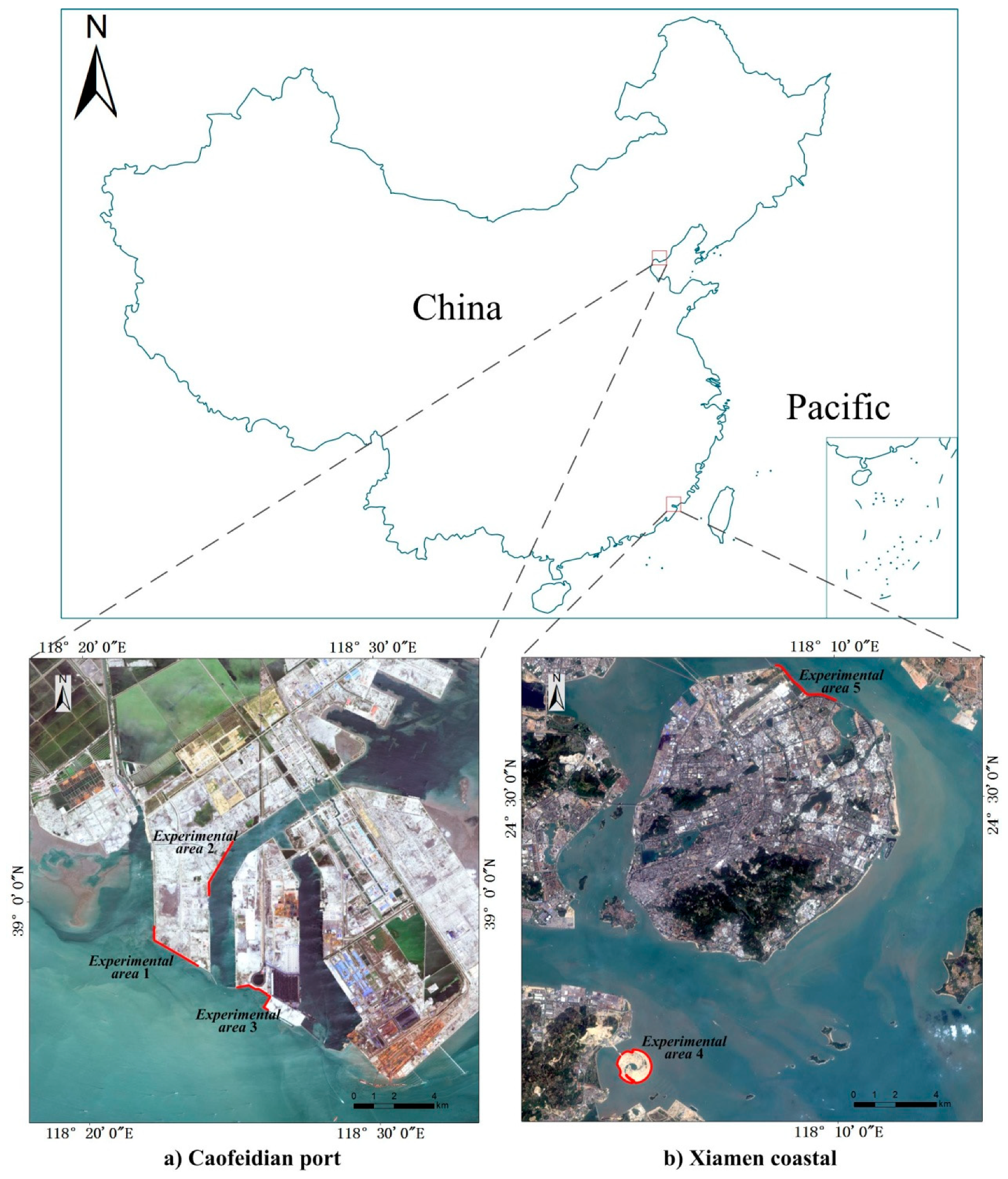
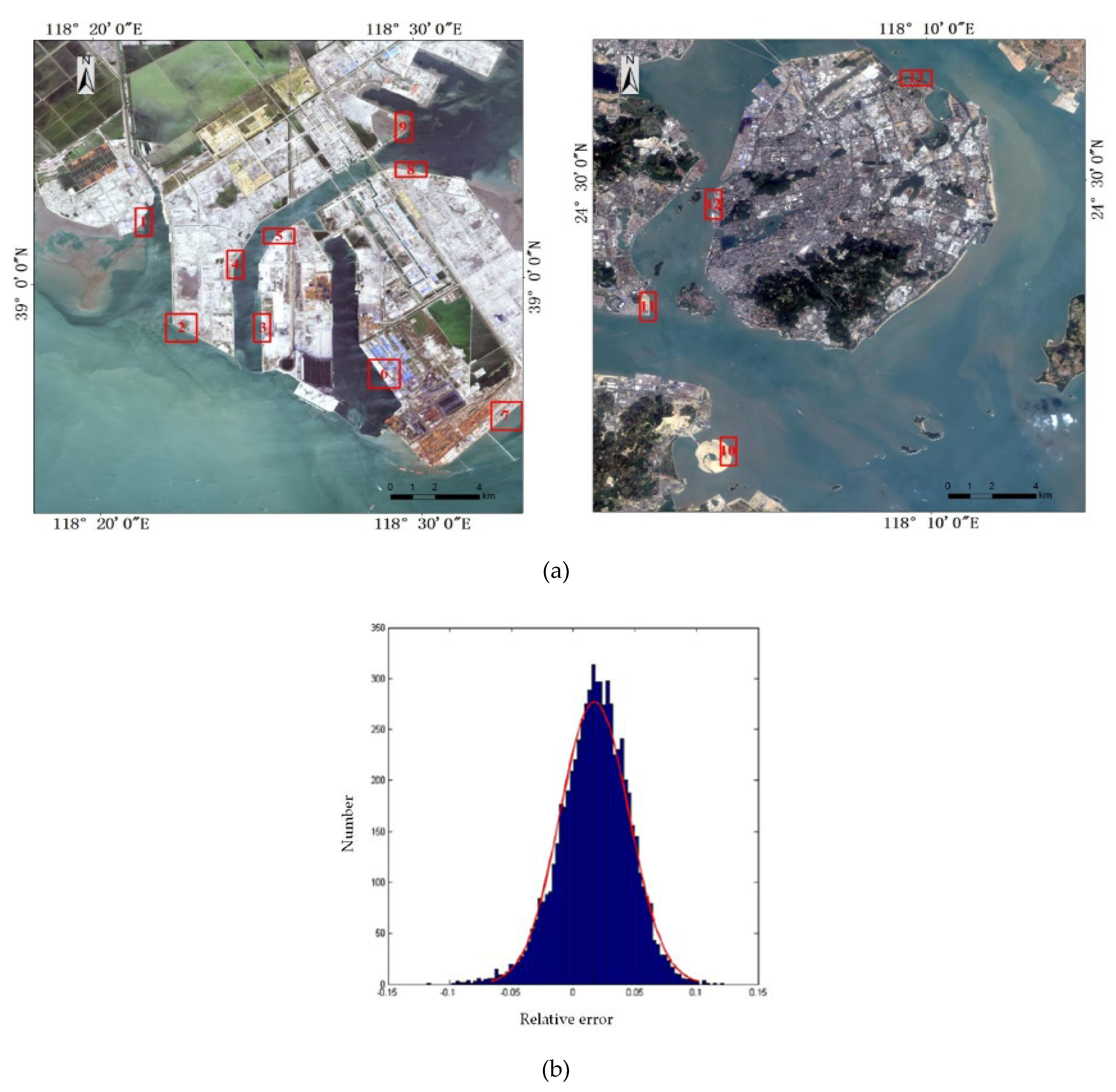
With urbanized development, there are increasingly more artificial shorelines located along Chinese coastal areas. Caofeidian Port and the Xiamen coastal area were selected as the study areas. As shown in Figure 1a, the Caofeidian Port located at 118.5°E, 39°N, is adjacent to China’s Beijing Tianjin Hebei urban agglomeration and is one of China’s important ore transportation ports. As shown in Figure 1b, the Xiamen coastal area, located between 118°E–118.5°E and 24.35°N–24.6°N, is next to the Taiwan Strait, and Xiamen is an important port for international economic and cultural exchange. Five artificial shorelines of various geometric morphologies as experimental areas were chosen to evaluate SGSSL, and their key characteristic parameters are listed in Table 1. The Gaofen-2 (GF-2) satellite data is selected as our reference data. GF-2 is the first civil optical remote sensing satellite independently developed by China with a spatial resolution better than 1 meter [41].
Our experiments verify the proposed algorithm from the following aspects. First, the subpixel shoreline localization results are superimposed on the original data to evaluate the visual effect of the proposed algorithm. Subsequently, compared with reference shoreline from GF-2, the four error indicators of the subpixel shoreline are calculated to verify the correctness and adaptability of the algorithm to different geometric morphology shorelines. Finally, the differences between the subpixel shoreline length and the reference shoreline length are calculated, which could illustrate ability of the proposed method to preserve details.
2.2. Data Pre-Processing
First, using the rational polynomial coefficient (RPC) of the GF-2 image, ortho-rectification of the GF-2 multi-spectral (MS) data and panchromatic (PAN) data were performed separately.
Then, the Gram Schmidt [42] pan sharpening algorithm was used to fuse the MS data with the PAN data; then, the spatial resolution of the Landsat 8 OLI fusion images was 15 m and that of the GF-2 fusion images was 1 m.
The registration parameters were estimated by correspondence feature points that were selected manually and by the polynomial model. The maximum registration error between the two fusion images (15 m/pixel fused Landsat8 OLI image, 1 m/pixel fused GF-2 image) is less than 3 m. The registration error will bring uncertainty to the accuracy assessment and is discussed in Section 5.1.
3. Materials and Methods
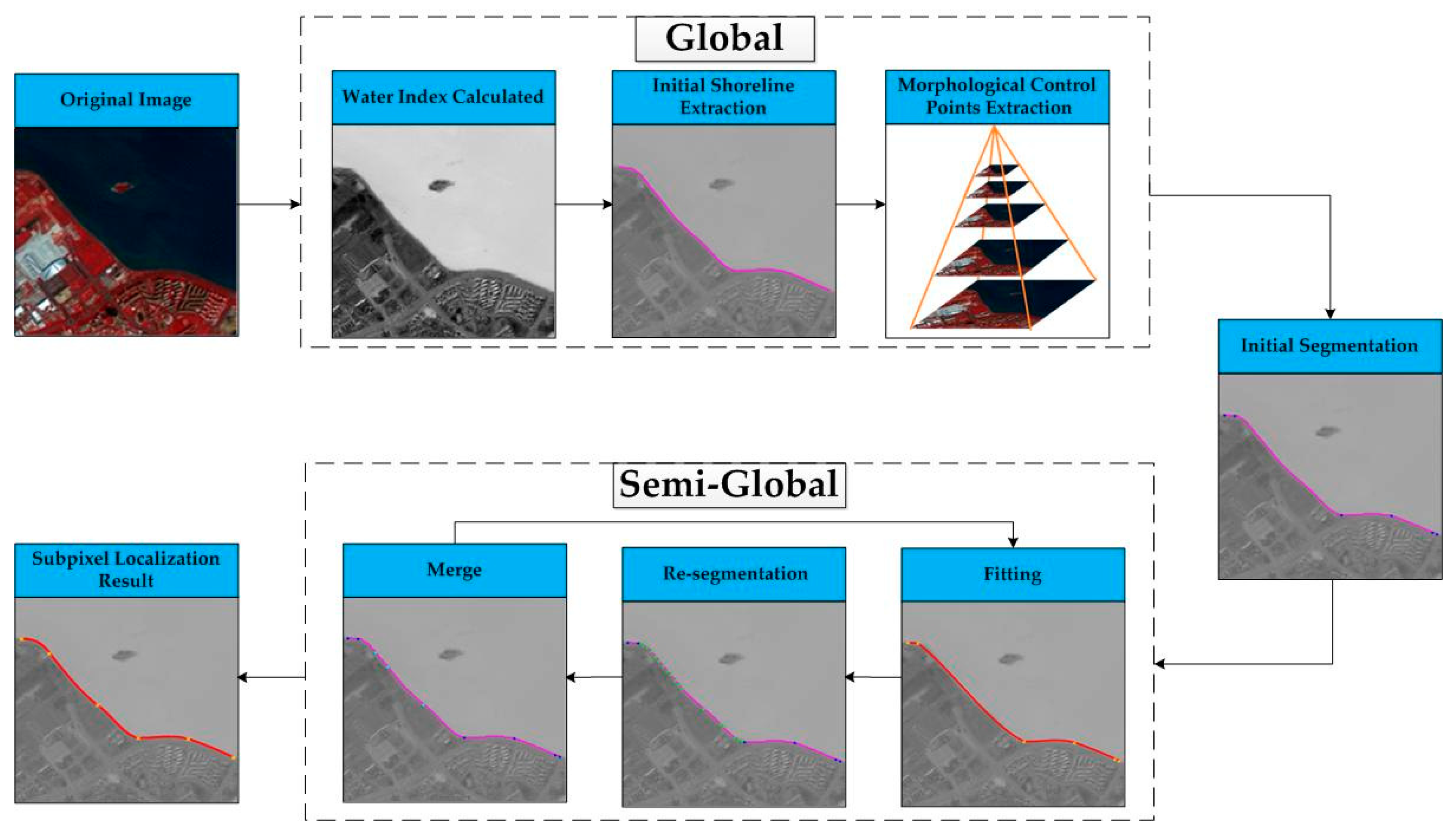
According to the main thoughts underlying SGSSL, the overall process is shown in Figure 2. First, global spectral and geometric morphology analysis are conducted: the initial shoreline is extracted using the Otsu [43] automatic threshold method from water index images; and geometric morphology control points, abbreviated as morphology control points (MCPs), are extracted using the multi-scale Harris algorithm [44]. The primary MCPs are utilized to divide the initial shoreline. Then, semi-global analysis is performed by the segmentation-merge-fitting (SMF) method. In the SMF process, the segmented shoreline subpixel location is determined by minimizing the intensity integral error, finally obtaining a continuous subpixel shoreline vector.
In Section 3.1, an ideal image is taken as an example to illustrate the basic principle of SGSSL. In Section 3.2, the challenges faced when the basic principle is applied to real satellite images are explained. In Section 3.3, the method of conducting the global analysis for SGSSL is introduced, including obtaining the initial shoreline position and extracting the MCPs. In Section 3.4, the process of performing a semi-global shoreline analysis for SGSSL is proposed, including designing local windows and details of the SMF processes.
3.1. Basic Principles of Subpixel Shoreline Localization
The entire shoreline can be regarded as consisting of many shoreline segments. The proposed subpixel shoreline localization algorithm is based on the following two assumptions:
Assumption 1: Any shoreline segment can be approximated by the polynomial function y = f(x).
Assumption 2: The shoreline segment divides the image into two homogeneous regions with intensities A and B (A < B).
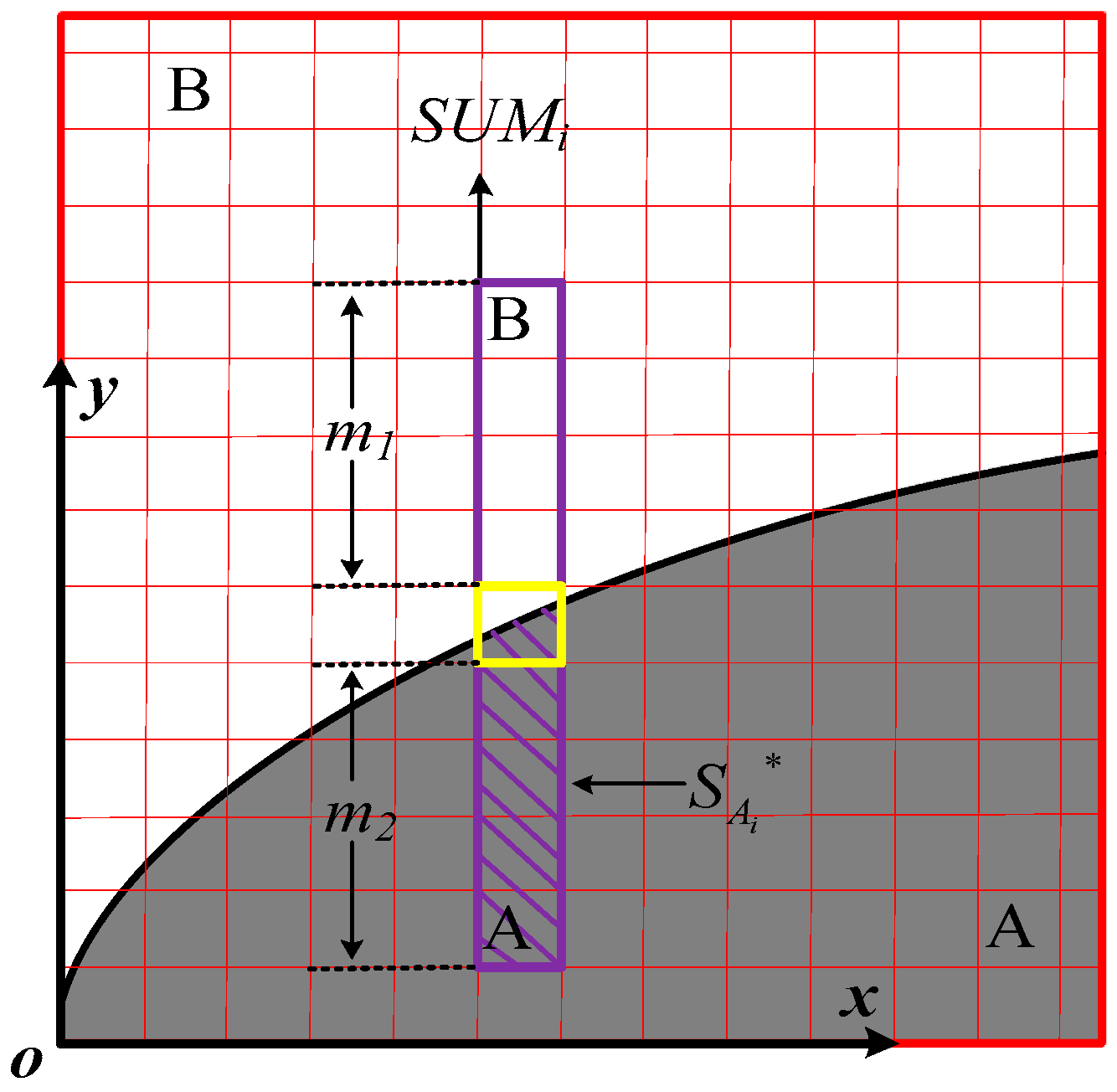
The ideal binary image is built in the image coordinate system O-xy, as shown in Figure 3, in which there is one shoreline segment.
A local window (the purple box in Figure 3) centered on the ith shoreline pixel (xi,yi) is set, so the sum of intensity in the ith window is:
where (xi,yi) is the current shoreline point’s pixel coordinate, G the pixel’s intensity, n the number of pixels in the shoreline segment, and m1, m2 are the pixels’ number above or under the shoreline csegment in the local window, respectively. According to Assumption 2, the integral of the intensity in the ith window is:
where and are areas covered by A or B in the local window, respectively:
According to Assumption 1, as the cubic function can express more geometric details and has superior morphological adaptability, the shoreline segment’s polynomial function is:
So, the area under the shoreline segment in the ith local window () can be calculated as:
With the above derivations, the intensity integral of the ith local window’s (SUMi*) can be described as:
In ideal conditions,
A similar idea has been researched by Trujillo-Pino et al. [36] for medical and indoor images, in which a subpixel edge location algorithm based on the partial area effect (PAE) was proposed. However, in that work, the algorithm neither considered the various geometric morphologies of the real shoreline/contour nor proved its application to actual satellite remote sensing images.
To solve Equation (7), the equation can be represented simply as:
where:
The following non-homogeneous equation can be obtained:
The intensity integral error in the ith local window (ei) is defined as:
By the least squares methodology, the cubic polynomial coefficients vector = (a,b,c,d)T can be solved with intensity integral error minimization, and then the shoreline subpixel localization is determined.
3.2. Challenges for Subpixel Shoreline Localization in Remote Sensing Images
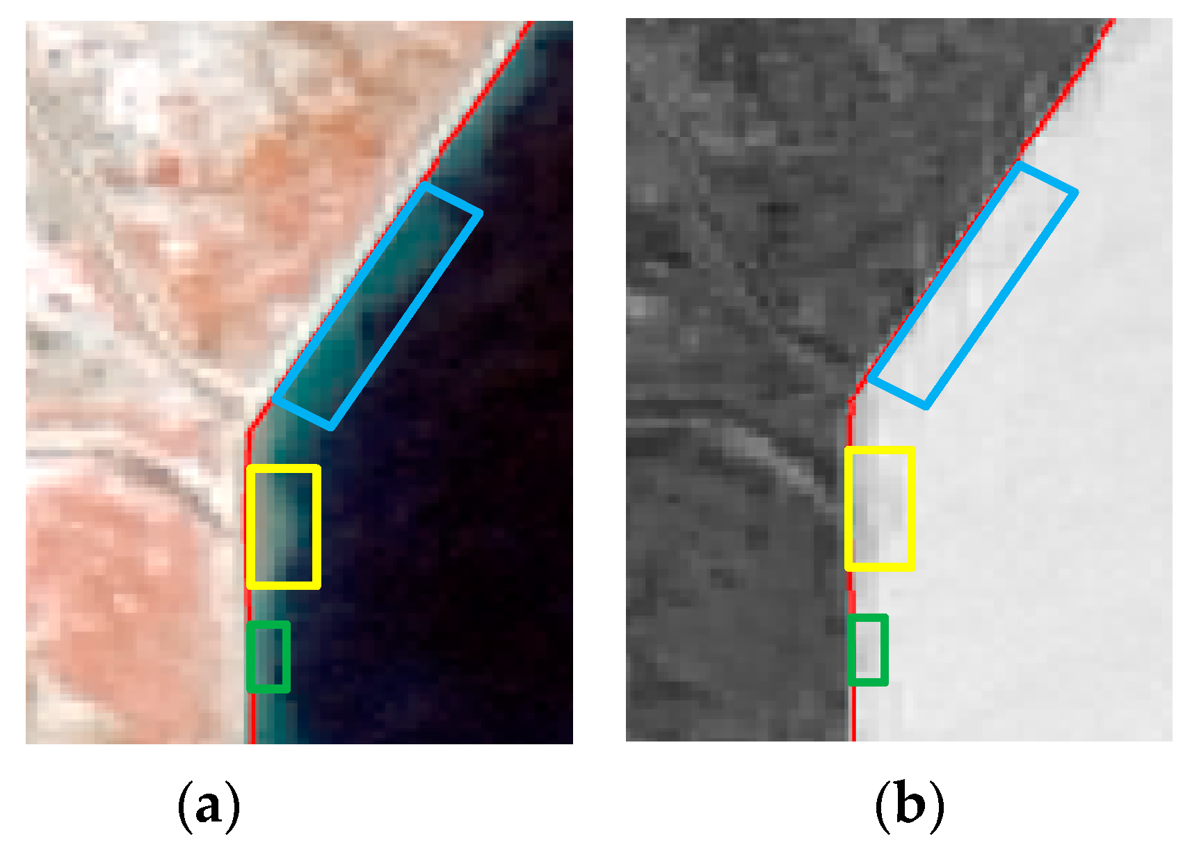
In Section 3.1, the derivation was based on the ideal image in Figure 3. When dealing with real shorelines, as Figure 4a shows, the initial shoreline (colored in purple) with various geometric morphologies does not satisfy Assumption 1. Therefore, the initial shoreline should be divided into segments of relatively simple morphologies, which can be approximated by the cubic polynomial function. For a shoreline to be divided appropriately, the multi-scale Harris corner algorithm [44] should be utilized to extract the MCPs.
When processing actual satellite images, the water index result is affected by sensor imaging noise and the interaction between adjacent classes. Meanwhile, heterogeneous pixels exist in the local window with intensity changes (Figure 4b, green box). Then, Assumption 2 is not satisfied, which leads to the intensity integral error expressed in Equation (10) not equaling zero.
It is therefore necessary to design the local window to guarantee the intensity integral error approaches zero to ensure the performance of SGSSL correctly.
3.3. Shoreline Global Analysis
3.3.1. Determination of Initial Shoreline Position
To make full use of satellite image global information, we will conduct a shoreline global analysis, which includes a spectral feature analysis and geometric morphology analysis to determine the initial shoreline position at the pixel level and extract appropriate MCPs.
3.3.2. Determination Initial Shoreline Position
Before extracting MCPs, we should determine the initial pixel level shoreline from the original fused satellite images. This procedure includes the following steps. First, the water index image is calculated. The modified normalized difference water index (MNDWI) [45] is preferred, and the reason why MNDWI is preferred is discussed in Section 5.1. Subsequently, the Otsu method [43] is applied to the water index image, in which an optimal threshold T* is selected automatically by maximizing the inter-class discrepancy. Third, using the optimal threshold value T*, the water index image is divided into a binary image, which includes non-water and water classes. A series of points representing the pixel level shoreline is obtained.
3.3.3. MCP Extraction
To satisfy Assumption 1, the initial pixel level shoreline with various geometric morphologies should be divided into segments with relatively simple morphology by MCPs. As multi-scale Harris detection [44] is sensitive to corners, MCPs are extracted by multi-scale Harris detection [44] from a binarized water index image:
where σI is the integral scale, g(σI) the Gaussian convolution kernel with integral scale σI, and La the derivative computed in the a direction. The multi-scale Harris cornerness measure combines the trace and the determinant of the scale-adapted second moment matrix:
where is an empirical coefficient, . It should be noted that decreasing the value of will increase the cornerness. Since our aim is to extract MCPs from the water/non-water binary image, the value of can be set to 0.06 (the maximum empirical value). The local maximum of cornerness at each scale determines the scales’ corner positions.
Second, each corner is verified depending on whether the Laplacian of Guassian (LOG) attains the maximum at the scale, and the LoG values are calculated by:
Comparing the LoG values with the adjacent two scale space images at the same position, if:
these corners would be reserved as multi-scale Harris corners.
Considering shoreline geometric morphological changes can be classified as dramatic variations and minor variations, the MCPs should include primary MCPs and supplementary MCPs. As the primary MCPs locate the positions at which the shoreline’s morphology changes drastically, theoretically, the multi-scale Harris corner points can be directly viewed as primary MCPs. However, during the process of building multi-scale image pyramids, images would be blurred and image structure details could be missed. Therefore, the initial scale’s corner subset is also preserved from multi-scale Harris detection [44] as supplementary MCPs. The partial area effect (PAE) subpixel algorithm [36] should be conducted for MCP positions to obtain their accurate subpixel position. These two types of MCPs and subpixel positions will be used in the SMF process.
3.4. Shoreline Semi-Global Analysis
To utilize the semi-global information of a shoreline segment correctly, we conduct shoreline semi-global analysis, which includes a designed local window and the SMF method to determine the local homogeneous intensity and obtain proper shoreline segments for subpixel localization.
3.4.1. Designing Local Window
In this subsection, we introduce how to design the local window [36] and estimate homogeneous intensities A and B [36] to ensure that the intensity integral error ei in Equation (10) is close to zero, so as to satisfy Assumption 2.
First, the maximum gradient direction of each shoreline point is calculated, and for every shoreline point, Sobel edge detection is utilized to calculate the gradient (Gx, Gy). Then, the larger gradient is preserved as the points’ maximum gradient direction.
It should be noted that the shoreline segment consists of numerous points. Therefore, if shoreline points of a certain maximum gradient direction (Gx or Gy) have a larger proportion in the segment, then that direction will be used as the main direction for the segment.
If the main direction for the segment is Gy, the (m1+m2+1) ×1 local window is designed, and the cubic polynomial function of a segment is:
If the main direction for the segment is Gx, the 1×(m1+m2+1) window is designed and the cubic polynomial function of segment is:
Second, since the homogeneous pixels’ intensities are stable, they have a minimum gradient in the local window’s direction. The algorithm adjusts m1, m2 to find the minimum gradient pixels (pixels in the blue box in Figure 4b). Once we find the minimum gradient pixels, their water index intensities are used to estimate the intensity A, B and their coordinates are used to set the window size [36].
In the ith window, the intensities Ai and Bi are the farthest pixels from the shoreline. To ensure the correlation between pixels in the local window, we limit .
Since there is a correlation between the intensities of adjacent points in the shoreline segment, to ensure that the homogeneity of A or B further prevents isolated noises, according to the adjacent shoreline points’ relative positions, we determine slope k of this shoreline point and calculate the more homogeneous intensity estimation values Ai* and Bi*:
where , (xi,yi) and (xi+1,yi+1) are the adjacent shoreline points’ coordinates.
3.4.2. Segmentation-Merge-Fitting Method
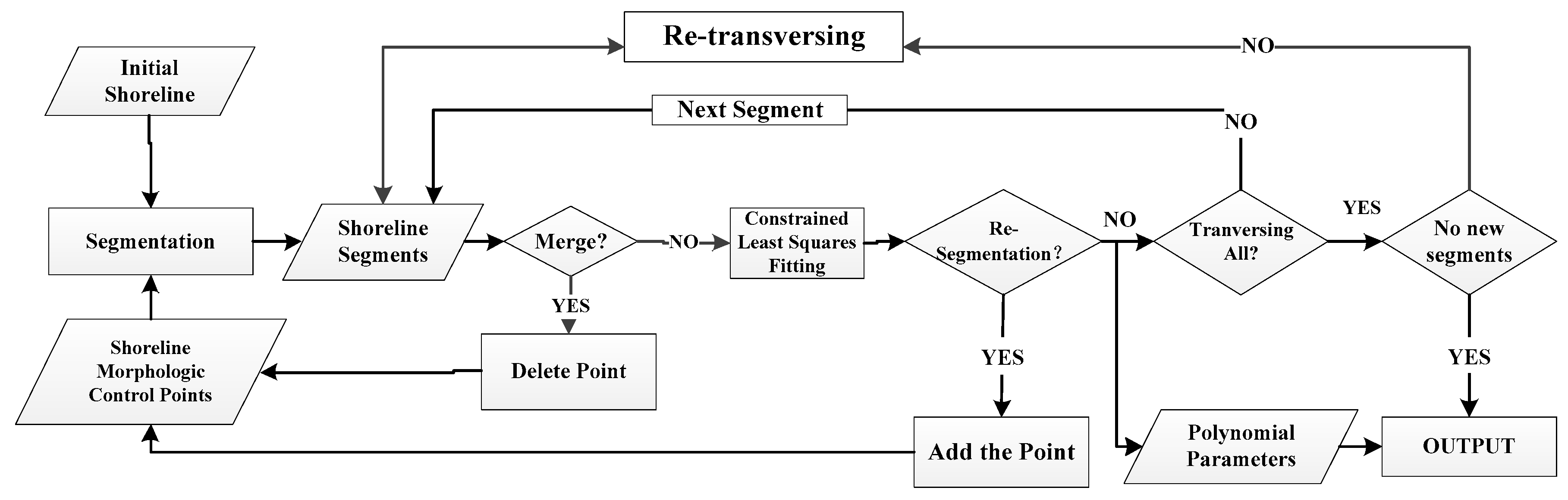
The MCPs determined in Section 3.3.2 include the primary MCPs and the supplementary MCPs, which have been derived from multi-scale Harris corners to represent the major and minor shoreline geometric morphologies. However, utilizing them all without any selection it will lead to over-segmented shorelines and a high computational burden for the subpixel localization algorithm. The segmentation-merge-fitting (SMF) method is proposed to obtain appropriate shoreline segments adaptively, according to the residuals of the least-squares process and the main directions of the adjacent shoreline segments. In the SMF, the least-squares fitting process and the subpixel positions of the MCPs are added as constraints (Equation (19)) to connect adjacent shoreline segments and obtain the continuous subpixel shoreline.
The detailed steps are shown in Figure 5.
The detailed explanation for all of the above steps follows:
0. Preparatory work: Build the shoreline morphological control point set (SMCPS) and add all primary MCPs to the SMCPS; set the threshold t of the least squares residual to 0.08.
1. Segmentation: Utilize the SMCPS to divide shoreline to obtain shoreline segments and calculate the main direction of each shoreline segment.
2. Merge: Judge whether the main direction of the current shoreline segment is the same as the main direction of the adjacent segment:
If TRUE, merge these two adjacent segments and go to the Step 3 ‘Delete Point’; else, go to Step 4.
3. Delete point: Remove the current morphological control point connecting the two adjacent segments from the SMCPS.
4. Fitting: Polynomial coefficients are calculated by the constrained least squares methodology, and the least squares residuals are computed for each point. If there are four shoreline points adjacent to the shoreline MCP, the residuals of which are larger than the threshold t, this shoreline MCP should be removed from the least square constraints. Then, the current shoreline segment must be recalculated. Else, go to Step 5.
5. Judge the ‘re-segmentation’ condition: If, in a shoreline segment, shoreline points with least-squares residuals larger than the threshold t continuously appear and these points’ number is larger than 4, the shoreline segment must be re-segmented. Go to Step 6; else go to Step 7.
6. Add Point:
① If the segment is a merged shoreline in Step 2, the MCPs removed in Step 2 should be restored in the SMCPS.
② If the segment is not a merged shoreline in Step 2, the supplementary MCPs located in the segment are added into the SMCPS.
③ If there are no supplementary MCPs in the segment, the point with the largest least squares residual should be selected and added into the SMCPS.
Update the SMCPS, and go to Step 1.
7. Traversing: If all shoreline segments have been traversed, keep the subpixel results and go to Step 8; else, select the next shoreline segment and go to Step 2.
8. End: If the SMCPS is constant during this traversal, end the loop and go to Step 9; else, go to the Step 2 and re-traverse.
9. Output: The subpixel shoreline results are output.
3.5. Verification Method
The reference shorelines are extracted manually from GF-2 fusion images, which satisfy the standards of the “Technical Regulations for Satellite Remote Sensing Survey on Island & Coastal Zones” [14]. Using the SGSSL algorithm, a subpixel shoreline can be obtained. The reference shoreline and the shoreline determined by SGSSL can be compared.
We choose four error indicators to assess the SGSSL performance: the MAE, RMSE, SD and LM. The MAE (Equation (20)) is obtained by averaging all distance errors, because all the errors are obtained by calculating the absolute value of the distance from the SGSSL shoreline to the GF-2 reference shoreline. The MAE and RMSE describe the SGSSL result bias towards the reference shoreline. The SD indicates the variability around the MAE (Equation (21)):
where is the distance from the subpixel shoreline point to the reference shoreline.
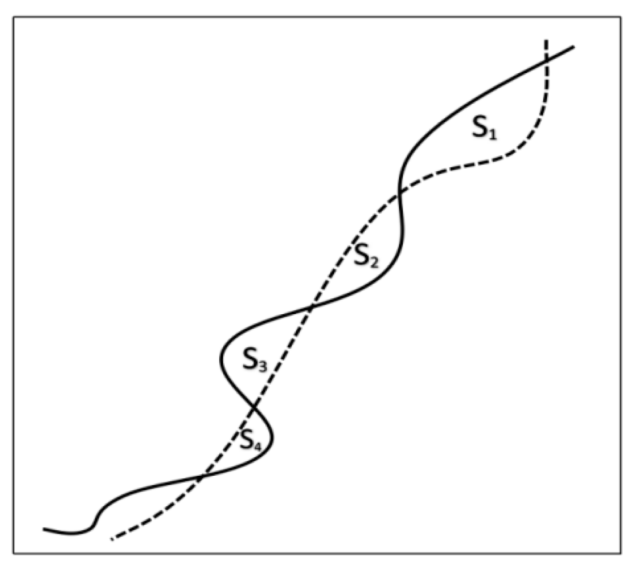
As Figure 6 shows, for the calculation of the LM [15], SΔ is the sum of the area enclosed by the SGSSL shoreline and the reference shoreline, and Lreal is the length of the reference shoreline. In Figure 6, the black dotted line represents the reference shoreline and the solid line represents the shoreline determined by SGSSL.
where .
4. Results
Here, we evaluate the results of the proposed SGSSL in terms of visual comparison, quantitative assessment, and shoreline detail preservation ability.
4.1. Visual Comparison
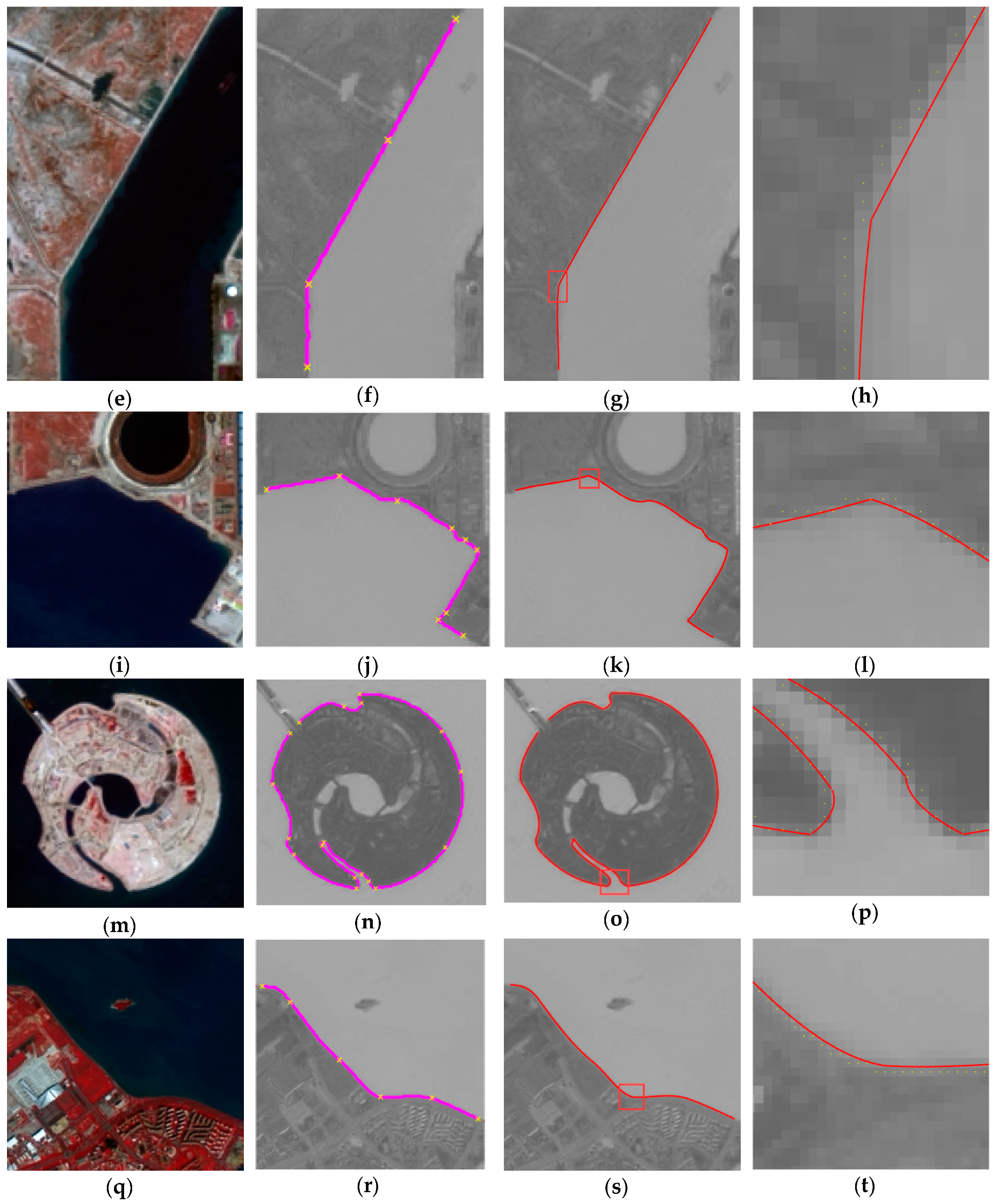
There are various geometric morphological shorelines in the selected coastal experimental areas. In the first two experimental areas (Figure 7a,e), the initial shoreline colored in purple has been extracted by Otsu [43] in Figure 7b,f. Owing to the fact that shoreline morphology is simple, MCPs labeled by yellow crosses can divide the initial shoreline into relatively simpler segments (Figure 7b,f). The proposed SGSSL algorithm determines the subpixel shoreline, which is represented by the red line in Figure 7c,g and which coincides with the real shoreline well. Although in the local zoomed image (Figure 7d,h) the initial pixel level shoreline points in yellow are located slightly landward, the final subpixel shoreline results (red line) still locate accurately.
In the latter three experimental areas (Figure 7i,m,q), the shoreline morphology is relatively complex, and the initial shoreline in purple has also been extracted by Otsu [43] in Figure 7 j,n,r. With the SMF method, we keep the selected MCPs labeled with yellow crosses (Figure 7j,n,r) and using them, the shoreline can be divided into relatively simpler segments to be perfectly expressed by red line in Figure 7k,o,s. Although in the local zoomed image (Figure 7l,p,t) the initial pixel level shoreline points in yellow are located slightly landward, the final subpixel shoreline results also coincide with the actual position well.
4.2. Quantitative Assessments
Table 2 summarizes the quantitative assessment results. In all experimental areas, the MAE at the subpixel level lies in the range of 2.48–3.34 m with an average of 3.03 m; the RMSE varies from 3.02–4.77 m with an average of 3.80 m; while the LM lies in the range of 2.51–3.72 m, with an average of 3.03 m. All quantitative assessments prove that the proposed SGSSL is reliable.
It should be noted that these assessment results may be affected by registration errors. How the registration errors influence the quantitative assessments is discussed in Section 5.1.
4.3. Shoreline Detail Preservation Ability
Some shoreline details observed in the high-resolution images would be blurred or missed in low-resolution images. Hence, it is necessary to verify the detail preservation ability of SGSSL for shoreline details by comparing the lengths between subpixel results and high-resolution images.
In Table 3, the length difference ratios between subpixel results and reference shorelines are calculated, and the maximum value is less than 2.5%, which indicates that the proposed SGSSL can effectively preserve shoreline details.
5. Discussion
5.1. Registration Error Influence on Quantitative Assessment
There are unavoidable registration errors when the accuracy assessment is conducted between the reference shorelines and SGSSL results. The registration errors will bring uncertainty to the quantitative assessment of SGSSL.
For objective analysis, three typical shoreline geometric morphologies are chosen for the registration error effect analysis.
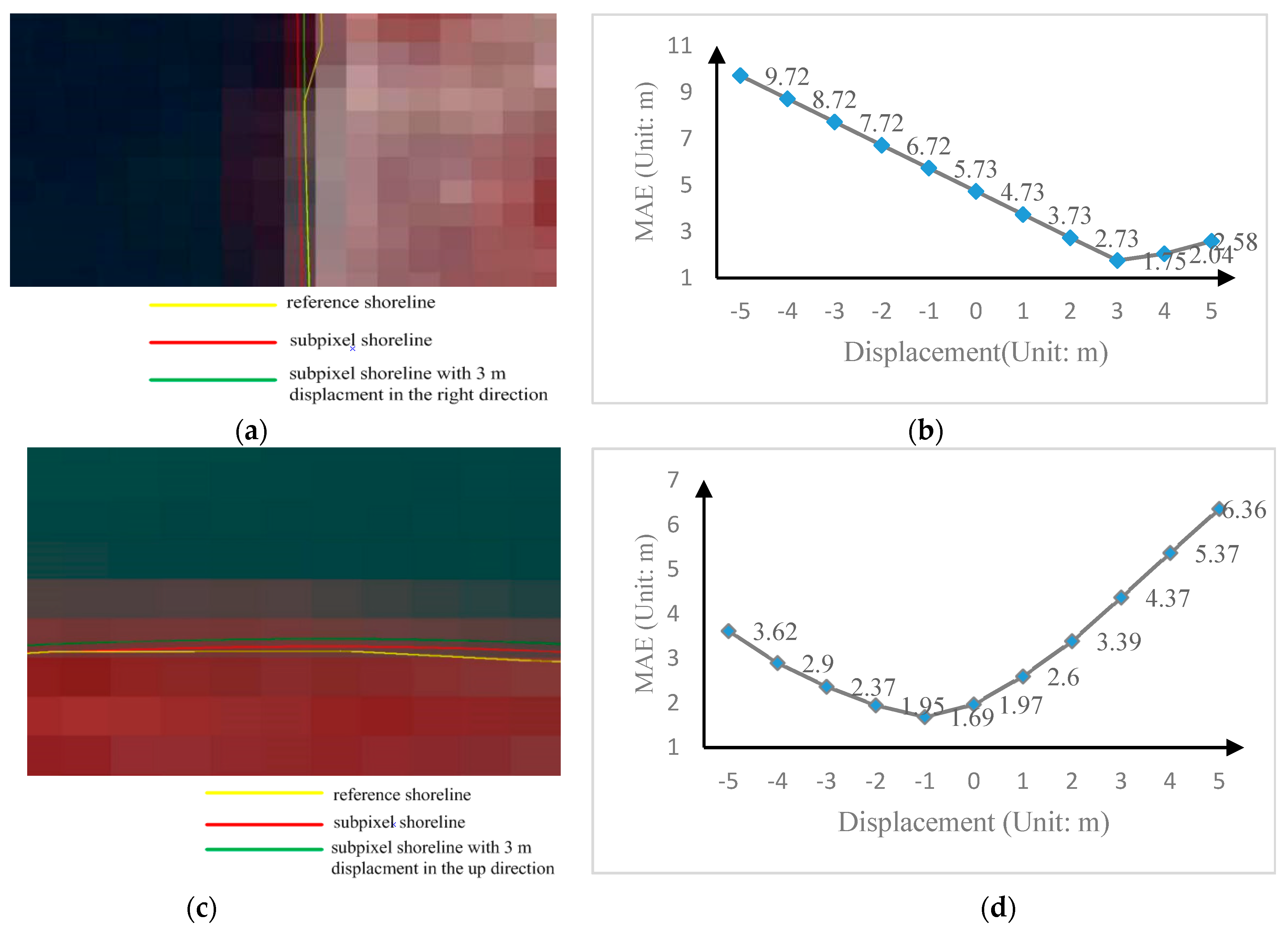
First, the upper part of experimental area 1 is chosen. Because the upper part of experimental area 1 is a nearly vertical shoreline, the displacement of the horizontal direction will bring an apparent influence to the final MAE. Using 1 m as the displacement interval (0.067 pixels for Landsat8 OLI data) and with the maximum displacement limited to 5 m, the registration error influence in the horizontal direction across the range of [–5 m, +5 m] can be calculated and observed in Figure 8a,b.
Second, the middle part of experimental area 5 is chosen. Because the middle part of experimental area 5 is a nearly horizontal shoreline, displacement in the vertical direction will bring an apparent effect on the final MAE. Using 1 m as the displacement interval (0.067 pixels for Landsat8 OLI data) and with the maximum displacement limited to 5 m, the registration error effect at the vertical direction in the range of [–5 m, +5 m] can be calculated and observed in Figure 8c,d.
As Figure 8a,b show, displacements in the right direction will compensate for the registration error influence on the MAE. The MAE without registration error compensation is 5.73 m, which is 2.59 m larger than the entire experimental area 1 MAE result. With registration error compensation in the right direction, the MAE decreases. At a displacement of 3 m in the right direction, the MAE is 2.73 m; at the same direction of displacement of 4 m, the MAE reaches its most accurate value, 1.75 m. After that, MAE results cannot be compensated.
As Figure 8c,d show, for the middle part of experimental area 5, displacement will also have an effect on the final MAE. The MAE is 1.69 m without any registration error compensation, which is smaller by 0.59 m than the entire MAE of experimental area 5. With displacements in the up or down directions, the worse MAE will be obtained. Additionally, at a displacement of 3 m in the up direction, the MAE is 3.39 m; at the displacement 3 m in the down direction, the MAE is 2.9 m.
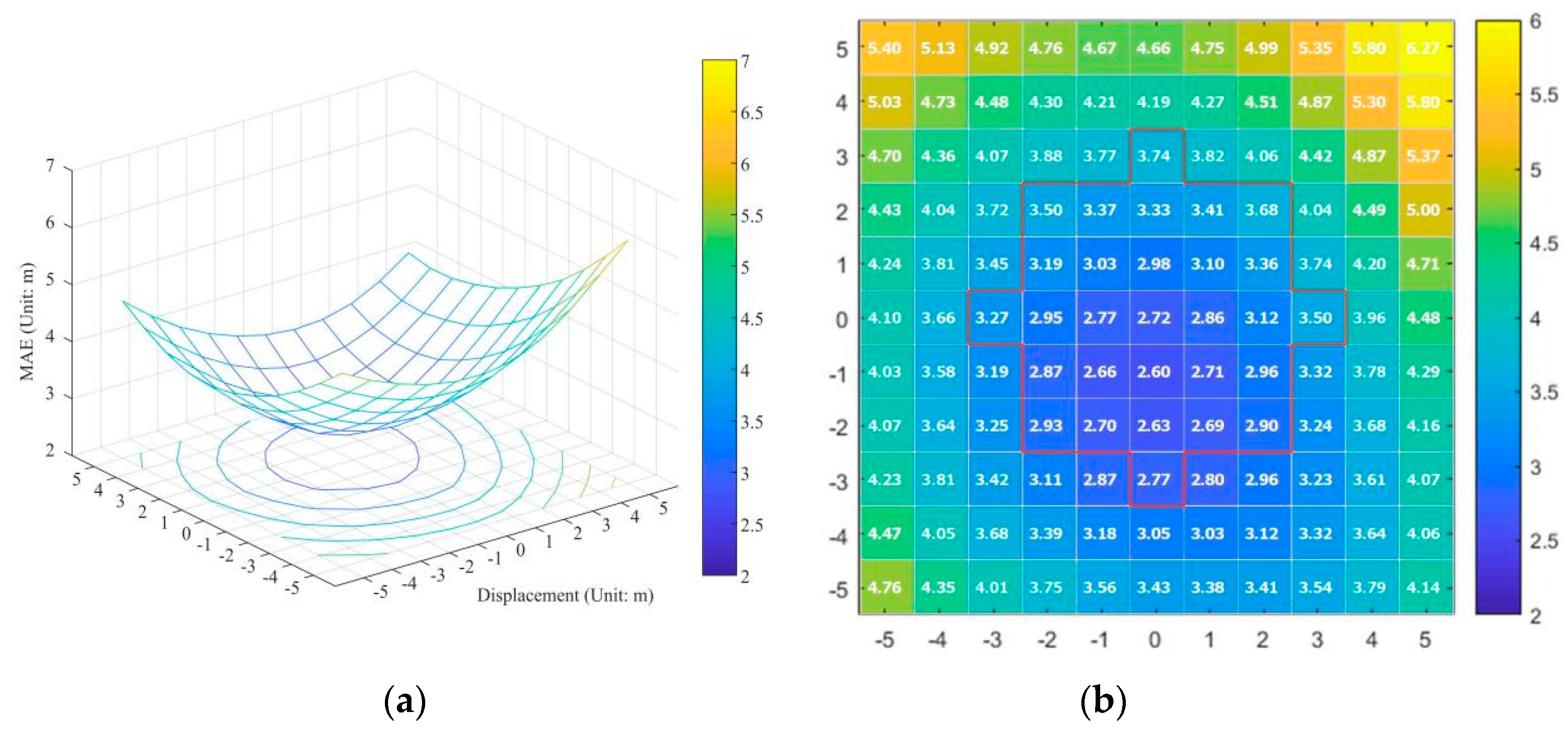
Third, experimental area 4 is chosen. Because the artificial shoreline in experimental area 4 is almost circular, the registration error will not influence the SGSSL result in certain directions. So the reference shoreline is displaced in four different directions, namely up, down, left and right, with 1 m of the displacement interval (0.067 pixels for Landsat8 OLI data), and the maximum displacement is limited to 5 m. In Figure 9, the MAE results of SGSSL with different displacements are shown.
From Figure 9, it can be observed that the MAE becomes more accurate in the 270° direction, namely in the down direction. The MAE first becomes most accurate at 2.60 m, which is the minimum MAE. The MAE then increases to 2.63 m in the 270° direction with a displacement of 2 m, and increases to 2.77 m in the same direction with a displacement of 3 m. For other directions, the MAE results are not better. The worst subpixel accuracy appears in the direction of 90°, the up direction, and the worst MAE is 3.74 m.
From the above analysis, it can be concluded that the registration error brings uncertainty to the SGSSL quantitative assessment results. With the same registration method, different geometric morphological shorelines are influenced by registration errors to different extents. The lowest accuracy of the MAE appears at the vertical shoreline, and the MAE reaches at 5.73 m, which is still better than 0.5 pixels (15 m of the fused Landsat8 OLI image). Hence, the registration error with a maximum value of less than 3 m is acceptable for SGSSL.
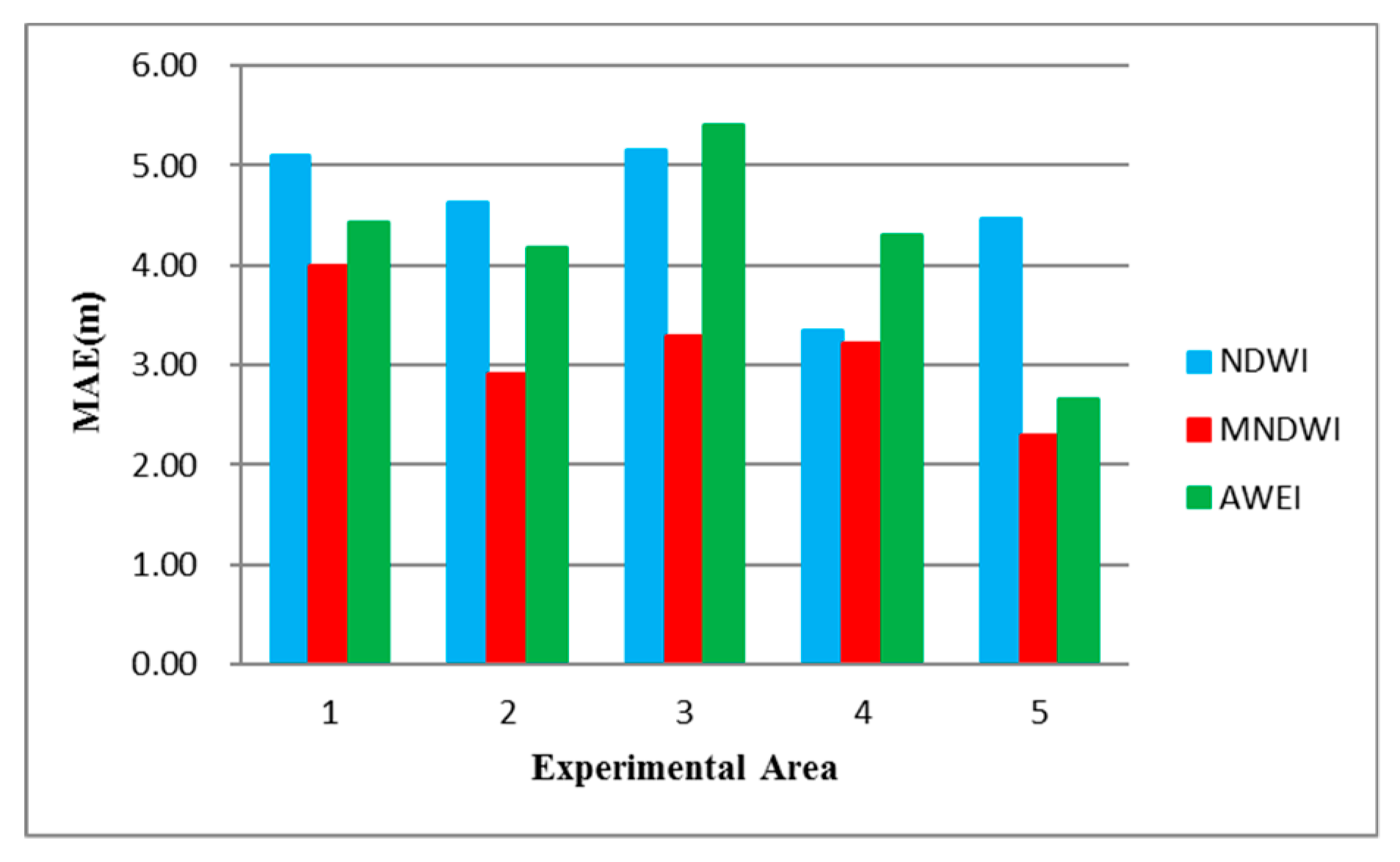
5.2. Water Index
To select the water index with optimal positioning accuracy, the positioning errors of the SGSSL algorithm under three different water indices—the normalized difference water index (NDWI) [46], MNDWI, and automated water extraction index (AWEI) [47]—are calculated and compared.
As Figure 10 shows, the accuracies of shoreline positioning under three different water indices have all reached the subpixel level, indicating that the proposed algorithm is applicable to all water indices. It is obvious that the MNDWI is best in the selected experimental areas. One of the reasons is that the short-wave infrared 1 (SWIR1,1566.50 – 1651.22 nm) band is used in the calculation of the MNDWI, and the most accurate and robust sub-pixel shoreline positioning results are often obtained using the SWIR1 band [40]. Therefore, this paper prefers to use the MNDWI to enhance the differences between land and water, but, considering complicated offshore environments and data sources, in other coastal areas utilizing other water indices is acceptable.
5.3. Intensity Integral Error Analysis
Owing to sensor imaging noise and the interaction between adjacent classes, the intensity integral error in the ith local window is probably not equal to zero.
As Figure 11 shows, the initial shoreline pixel coordinate is (xi,yi), and the red line is the real shoreline that crosses the pixel (xi,yi). The subpixel level coordinates of the point in the real shoreline are (x0,y0), (x0∈[xi−1/2, xi+1/2], y0∈[yi−1/2, yi+1/2]). Once the local window size is determined by finding the minimum gradient pixels along the window direction, the window sizes m1, m2 and the homogeneous intensity Ai, Bi are all obtained. At shoreline point (x0,y0), the intensity profile is drawn along the window direction, presuming the direction lies in the y axes in Figure 11.
If the shoreline segment can be expressed by a cubic polynomial. S1,S2,S3 are areas enclosed by the intensity profile and the y axis (window direction),
Therefore, the sum of the ith local window intensity is:
where, in the local window, G is the pixel intensity. The approximation of the sum of the ith local window intensity is:
Thus, in the local window the intensity integral error ei can be described as:
where the intensity integral error ei is related to three factors: the window size (m1+m2+1), the homogeneous intensity difference (B-A), and the intensity slope at the shoreline point (x0,y0). Regarding the three factors, the intensity slope is determined by image information. The other two factors are determined by appropriate homogeneous intensity estimation A, B and the window’s size (m1+m2+1), which can ensure that the ei approaches zero.
Furthermore, to verify the correctness of the local window design method and to verify whether or not the intensity integral error ei approaches zero, the relative error δ is calculated within the local window in Landsat OLI8 MNDWI images.
The shorelines extracted manually from GF-2 images are viewed as the reference shorelines. In Equation (28), SUMi* is the integral of intensity in the ith window and calculated according to Equation (6). The reference shoreline coordinates are used to calculate S*Ai and S*Bi. SUMi is the sum of intensity in the ith window and calculated according to Equation (3).
As Figure 12a shows, 6743 local windows covering different offshore environments over different periods of time in the study areas were sampled. The relative error distribution is shown in Figure 12b, the mean of δ is 0.0174 and the variance is 0.0278. The probability of δ less than 5% is 87.57%, and that of δ being less than 10% is 99.85%. Thus, it can be concluded that in most local windows, the relative error δ can be seen as a small number, whose absolute value approaches zero.
5.4. Segmentation-Merge-Fitting Process
As mentioned in Section 3.4.2, the initial shoreline may not be perfectly expressed by the cubic polynomial function. In Figure 13a, it can be observed that the initial shoreline could be divided into relatively simpler segments by primary MCPs (colored blue). As shown in Figure 13b,c (a magnified version of Figure 13b), after using primary MCPs and constrained least squares solving, one shoreline segment containing many shoreline points of larger fitting residuals still exists (marked by the yellow box in Figure 13b), which must be segmented further. In Figure 13d, all supplementary MCPs in green would be used to re-segment this problematic segment. Then, as the Figure 13e shows, some segments would be merged. Finally, appropriate shoreline segments that perfectly agree with polynomial functions are obtained using the SMF method, and are named seg1–seg3 in Figure 13f, the final SMCPS selected from MCPs are labeled by yellow crosses. As shown in Figure 13g,h (a magnified version of Figure 13g), the final subpixel positioning results coincide well with the real shoreline position.
Table 4 lists the subpixel assessment indicators (MAE and SD) of shoreline segments marked by yellow boxes in Figure 13 during the SMF process. For the initial longer shoreline segment divided by primary MCP, the MAE and SD of subpixel localization results are 10.53 m and 12.11 m, respectively, which indicate that the initial subpixel localization result is problematic. With the SMF process, the final selected MCPs distribute appropriately along the shoreline and three correct segments are preserved. In addition, the subpixel localization MAE results lie in the range of 2.12 m to 3.22 m and the SD results from 1.84 m to 2.20 m.
5.5. Robustness to Complex Offshore Environment and Salt-And-Pepper Noises
In Figure 14, due to the complex offshore environment, for example, the existence of suspended sediment (Figure 14a), the local window is difficult to obtain, which will directly affect the subpixel localization accuracy.
In Figure 14a,b, suspended sediment situations can be grouped into three different categories depending on the concentration extent and accumulated area.
When the suspended sediment concentration is low (the regions in the blue boxes in Figure 14), the influence will be suppressed or even eliminated in MNDWI images, regardless of the size of the accumulated area.
When the suspended sediment concentration is high and the accumulated area is small with a width less than four pixels, this region (green boxes in Figure 14) will be regarded as the intensity variation region in the local window. In this situation, with the local window design method, the minimum gradient pixels would be found in water, whose intensity is homogeneous.
When the suspended sediment concentration is high and the accumulated area is large (in yellow boxes in Figure 14), with the local window design method, the homogeneous pixels will be selected directly in the suspended sediment region.
In conclusion, regarding the above three forms of suspended sediments, the homogeneous intensity estimations are dealt with effectively and will not reduce the subpixel localization accuracy.
Table 5 summarizes the MAE results of the selected local suspended sediment region, which lie in the range of 0.96–3.55 m, proving that our proposed SGSSL is robust to suspended sediments to some degree.
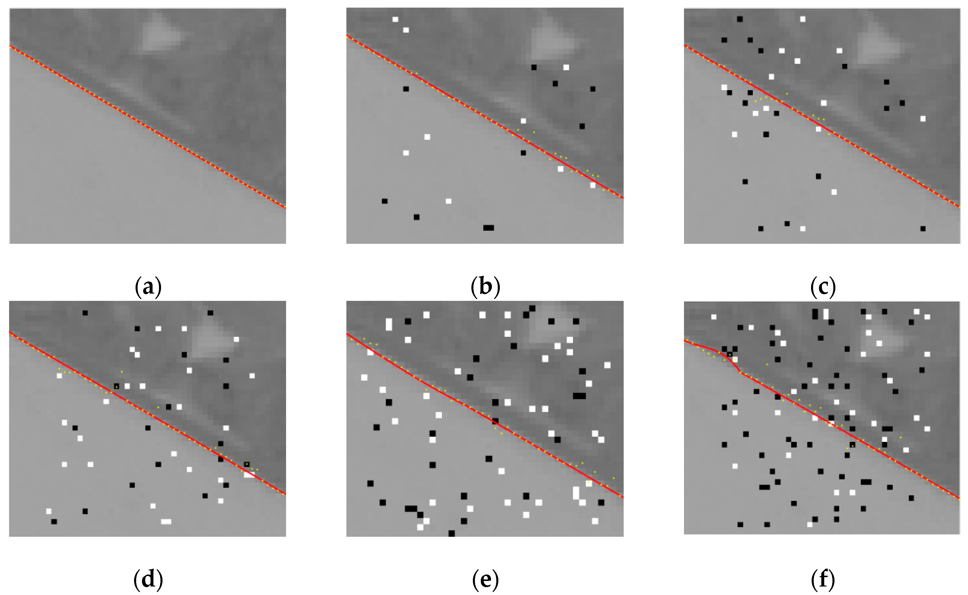
Furthermore, we evaluate the proposed SGSSL performance under the influence of salt-and-pepper noises. In Figure 15, the yellow points are determined by the PAE subpixel algorithm proposed by Trujillo-Pino [36], and the red lines are determined from SGSSL, where the white and black points are salt-and-pepper noise. With increasing noise percentage, the PAE subpixel results become increasingly problematic. However, the results determined by SGSSL are always accurate and are not affected by increasing salt-and-pepper noise.
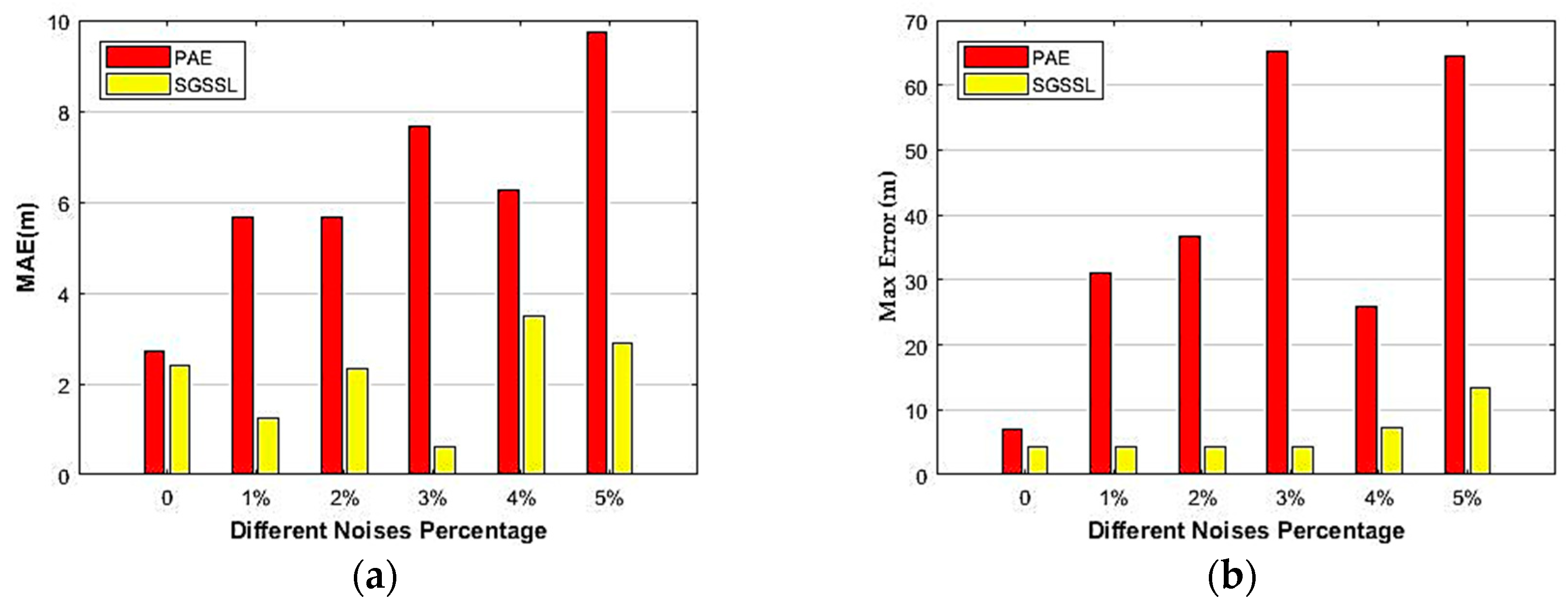
As shown in Figure 16, the positioning accuracy results of the two methods under different percentages of salt-and-pepper noise are quantitatively evaluated. With increasing noise percentage, it is obvious that the SGSSL algorithm exhibits better accuracy, proving that the proposed SGSSL is robust to salt-and-pepper noise to some extent.
6. Conclusions
With the merits of efficient, large-scale investigational capability, satellite remote sensing shoreline mapping plays an important role in the monitoring of coastal resource management. However, low spatial resolution, various shoreline geometric morphologies, and complex offshore environments prevent the accurate positioning of shorelines. In this study, therefore, we proposed a semi-global subpixel shoreline localization (SGSSL) algorithm for accurately determining artificial shorelines.
The proposed method utilizes not only global spectral information and shoreline morphological features, but also local water index homogeneity features and simplifies the entire shoreline subpixel positioning problem with a segmented shoreline fitting solution. The method considers the following factors: (1) MCPs are utilized to divide the initial shoreline into segments of relatively simple geometric morphology; (2) minimum gradient pixels are found to design a local window; (3) the intensity integral error is minimized in every local window within a segment to initially determine the subpixel location; and (4) the SMF process is presented to obtain the shoreline segments that can be perfectly expressed by a cubic polynomial function and to determine the final subpixel results.
In experiments, five artificial shorelines of various geometric morphologies from Landsat 8 OLI images were selected. The accuracy of the proposed method was evaluated using four error indicators: the MAE, SD, RMSE, and LM. The subpixel RMSE results are all less than 5 m, ranging from 3.02–4.77 m; and the LM results are all less than 4 m, ranging from 2.51–3.72 m, proving that subpixel shoreline accuracy obtained by the proposed method is stable over different experimental areas with various morphologies.
It can be concluded that the proposed algorithm is applicable to the various geometric morphologies of artificial shorelines and is robust to complex offshore environments and salt-and-pepper noise, to some extent.
Limitations of the proposed algorithm include the fact that its performance heavily depends on MCP distribution. Although the SMF process helps in obtaining optimum segments, in some experimental images a lack of MCPs will lead to irreparable subpixel accuracy loss. Another issue worth mentioning is that the proposed algorithm relies on the initial pixel level shoreline, which is the local window determination basis. More adaptation thresholding methodology should be applied to guarantee the initial pixel level shoreline’s correct position. Finally, the proposed SGSSL has only been verified on a selected artificial shoreline, other types of shoreline, for example, sandy shorelines and mangrove shorelines, have not been evaluated.
In future research, the performance of the method should be improved by a more flexible MCP extraction algorithm and a more reliable initial shoreline determination method. In terms of application prospects, the method will be combined with multi-source satellite images or ground truth data in the continuous monitoring of shoreline dynamics, coastal terrain mapping and other related research topics.
Author Contributions
Y.S. conceived the idea of the study and designed it. L.F. conducted the experiments. F.L proposed the study on morphological control point distribution and method of how to verify the algorithms effectiveness. L.W.Y help to design the study and verify the results. All authors contributed equally, analyzed the data.
Funding
This work was supported by the Opening Fund of Key Laboratory of Geological Survey and Evaluation of Ministry of Education (Grant No. CUG2019ZR09) and the Fundamental Research Funds for the Central Universities. And this work was also supported by Natural Science Fund of Hubei Province (No.2016CFB690) and the Fund of Key Laboratory of Technology for Safeguarding of Maritime Rights and Interests and Application (No. SCS1610).
Acknowledgments
The authors would like to thank Haitian Zhu (National Satellite Ocean Application Service) for his useful comments from a coastal engineering point of view.
Conflicts of Interest
The authors declare no conflict of interest. The funders had no role in the design of the study; in the collection, analyses, or interpretation of data; in the writing of the manuscript, nor in our decision to publish the results.
References
- Liu, Y.; Wang, X.; Ling, F.; Xu, S.; Wang, C. Analysis of Coastline Extraction from Landsat-8 OLI Imagery. Water 2017, 9, 816. [Google Scholar] [CrossRef]
- Aedla, R.; Dwarakish, G.S.; Reddy, D.V. Automatic shoreline detection and change detection analysis of Netravati-Gurpur River mouth using histogram equalization and adaptive thresholding techniques. Aquat. Procedia 2015, 4, 563–570. [Google Scholar] [CrossRef]
- Moore, L.J. Shoreline mapping techniques. J. Coast. Res. 2000, 16, 111–124. [Google Scholar]
- Lira, C.P.; Silva, A.N.; Taborda, R.; de Andrade, C.F. Coastline evolution of Portuguese low-lying sandy coast in the last 50 years: An integrated approach. Earth Syst. Sci. Data 2016, 8, 265–278. [Google Scholar] [CrossRef]
- Caixia, Y.U.; Wang, J.; Jun, X.U.; Peng, R.; Cheng, Y.; Wang, M.; Academy, D.N. Advance of Coastline Extraction Technology. J. Geomater. Sci. Technol. 2014, 31, 305–309. (In Chinese) [Google Scholar]
- Dewi, R.; Bijker, W.; Stein, A.; Marfai, M. Flzzy Classification for Shoreline Change Monitoring in a Part of the Northern Coastal Area of Java, Indonesia. Remote Sens. 2016, 8, 190. [Google Scholar] [CrossRef]
- Boak, E.H.; Turner, I.L. Shoreline Definition and Detection: A Review. J. Coast. Res. 2005, 214, 688–703. [Google Scholar] [CrossRef]
- Alesheikh, A.A.; Ghorbanali, A.; Nouri, N. Coastline change detection using remote sensing. Int. J. Environ. Sci. Technol. 2007, 4, 61–66. [Google Scholar] [CrossRef] [Green Version]
- Li, W.; Gong, P. Continuous monitoring of coastline dynamics in western Florida with a 30-year time series of Landsat imagery. Remote Sens. Environ. 2016, 179, 196–209. [Google Scholar] [CrossRef]
- Shearman, P.; Bryan, J.; Walsh, J.P. Trends in Deltaic Change over Three Decades in the Asia—Pacific Region. J. Coast. Res. 2013, 290, 1169–1183. [Google Scholar] [CrossRef]
- Le Cozannet, G.; Garcin, M.; Yates, M.; Idier, D.; Meyssignac, B. Approaches to evaluate the recent impacts of sea—Level rise on shoreline changes. Earth-Sci. Rev. 2014, 138, 47–60. [Google Scholar] [CrossRef]
- Bird, E.C.F. The modern prevalence of beach erosion. Mar. Pollut. Bull. 1987, 18, 151–157. [Google Scholar] [CrossRef]
- Gens, R. Remote sensing of coastlines: Detection, extraction and monitoring. Int. J. Remote Sens. 2010, 31, 1819–1836. [Google Scholar] [CrossRef]
- State Oceanic Administration 908 Special Office. Technical Regulations for Satellite Remote Sensing Survey on Island Coastal Zone; Ocean Press: Beijing, China, 2005; ISBN 9787502764852. (In Chinese) [Google Scholar]
- Wang, C.; Zhang, J.; Ma, Y. Coastline interpretation from multispectral remote sensing images using an association rule algorithm. Int. J. Remote Sens. 2010, 31, 6409–6423. [Google Scholar] [CrossRef]
- Li, X.; Ling, F.; Du, Y.; Feng, Q.; Zhang, Y. A spatial–temporal Hopfield neural network approach for super—Resolution land cover mapping with multi—Temporal different resolution remotely sensed images. ISPRS J. Photogramm. 2014, 93, 76–87. [Google Scholar] [CrossRef]
- Kasetkasem, T.; Arora, M.; Varshney, P. Super-resolution land cover mapping using a Markov random field based approach. Remote Sens. Environ. 2005, 96, 302–314. [Google Scholar] [CrossRef]
- Tolpekin, V.A.; Stein, A. Quantification of the effects of land-cover-class spectral separability on the accuracy of Markov-random-field-based super resolution mapping. IEEE Trans. Geosci. Remote Sens. 2009, 47, 3283–3297. [Google Scholar] [CrossRef]
- Ling, F.; Du, Y.; Xiao, F.; Li, X. Subpixel Land Cover Mapping by Integrating Spectral and Spatial Information of Remotely Sensed Imagery. IEEE Geosci. Remote Sens. Lett. 2012, 9, 408–412. [Google Scholar] [CrossRef]
- Zhang, Y.; Du, Y.; Li, X.; Fang, S.; Ling, F. Unsupervised Subpixel Mapping of Remotely Sensed Imagery Based on Fuzzy C-Means Clustering Approach. IEEE Geosci. Remote Sens. Lett. 2014, 11, 1024–1028. [Google Scholar] [CrossRef]
- Atkinson, P.M. Sub-pixel Target Mapping from Soft-classified, Remotely Sensed Imagery. Photogramm. Eng. Remote Sens. 2015, 71, 839–846. [Google Scholar] [CrossRef]
- Ge, Y.; Li, S.; Lakhan, V.C. Development and Testing of a Subpixel Mapping Algorithm. IEEE Trans. Geosci. Remote Sens. 2009, 47, 2155–2164. [Google Scholar]
- Su, Y.; Foody, G.M.; Muad, A.M.; Cheng, K. Combining Hopfield Neural Network and Contouring Methods to Enhance Super-Resolution Mapping. IEEE J.-STARS 2012, 5, 1403–1417. [Google Scholar]
- Ling, F.; Du, Y.; Li, X.; Li, W.; Xiao, F.; Zhang, Y. Interpolation-based super-resolution land cover mapping. Remote Sens. Lett. 2013, 4, 629–638. [Google Scholar] [CrossRef]
- Li, X.; Ling, F.; Du, Y.; Zhang, Y. Spatially Adaptive Superresolution Land Cover Mapping with Multispectral and Panchromatic Images. IEEE Trans. Geosci. Remote Sens. 2014, 52, 2810–2823. [Google Scholar] [CrossRef]
- Li, X.; Du, Y.; Ling, F. Super-Resolution Mapping of Forests With Bitemporal Different Spatial Resolution Images Based on the Spatial-Temporal Markov Random Field. IEEE J.-STARS 2014, 7, 29–39. [Google Scholar]
- Chen, Y.; Ge, Y.; Heuvelink, G.B.M.; Hu, J.; Jiang, Y. Hybrid Constraints of Pure and Mixed Pixels for Soft-Then-Hard Super-Resolution Mapping with Multiple Shifted Images. IEEE J.-STARS 2015, 8, 2040–2052. [Google Scholar] [CrossRef]
- Shi, Z.; Li, P.; Jin, H.; Tian, Y.; Chen, Y.; Zhang, X. Improving Super-Resolution Mapping by Combining Multiple Realizations Obtained Using the Indicator—Geostatistics Based Method. Remote Sens. 2017, 9, 773. [Google Scholar] [CrossRef]
- Chen, Y.; Ge, Y.; An, R.; Chen, Y. Super-Resolution Mapping of Impervious Surfaces from Remotely Sensed Imagery with Points-of-Interest. Remote Sens. 2018, 10, 242. [Google Scholar] [CrossRef]
- Ling, F.; Li, X.; Xiao, F.; Du, Y. Super resolution Land Cover Mapping Using Spatial Regularization. IEEE Trans. Geosci. Remote Sens. 2014, 52, 4424–4439. [Google Scholar] [CrossRef]
- Foody, G.M.; Muslim, A.M.; Atkinson, P.M. Super-resolution mapping of the waterline from remotely sensed data. Int. J. Remote Sens. 2007, 26, 5381–5392. [Google Scholar] [CrossRef]
- Muslim, A.M.; Foody, G.M.; Atkinson, P.M. Localized soft classification for super-resolution mapping of the shoreline. Int. J. Remote Sens. 2007, 27, 2271–2285. [Google Scholar] [CrossRef]
- Muslim, A.M.; Foody, G.M.; Atkinson, P.M. Shoreline Mapping from Coarse–Spatial Resolution Remote Sensing Imagery of Seberang Takir, Malaysia. J. Coast. Res. 2007, 236, 1399–1408. [Google Scholar] [CrossRef]
- Zhang, Y. Super-resolution mapping of coastline with remotely sensed data and geostatistics. J. Remote Sens. 2010, 14, 157–172. [Google Scholar]
- Liu, Q.; Trinder, J.; Turner, I. A Comparison of Sub-Pixel Mapping Methods for Coastal Areas. ISPRS Ann. Photogramm. Remote Sens. Spat. Inf. Sci. 2016, III-7, 67–74. [Google Scholar] [CrossRef]
- Trujillo-Pino, A.; Krissian, K.; Alemán-Flores, M.; Santana-Cedrés, D. Accurate subpixel edge location based on partial area effect. Image Vis. Comput. 2013, 31, 72–90. [Google Scholar] [CrossRef]
- Pardo-Pascual, J.E.; Almonacid-Caballer, J.; Ruiz, L.A.; Palomar-Vázquez, J. Automatic extraction of shorelines from Landsat TM and ETM+ multi-temporal images with subpixel precision. Remote Sens. Environ. 2012, 123, 1–11. [Google Scholar] [CrossRef] [Green Version]
- Almonacid-Caballer, J.; Sánchez-García, E.; Pardo-Pascual, J.E.; Balaguer-Beser, A.A.; Palomar-Vázquez, J. Evaluation of annual mean shoreline position deduced from Landsat imagery as a mid-term coastal evolution indicator. Mar. Geol. 2016, 372, 79–88. [Google Scholar] [CrossRef]
- Liu, Q.; Trinder, J.; Turner, I.L. Automatic super-resolution shoreline change monitoring using Landsat archival data: A case study at Narrabeen-Collaroy Beach, Australia. J. Appl. Remote Sens. 2017, 11, 16036. [Google Scholar] [CrossRef]
- Pardo-Pascual, J.; Sánchez-García, E.; Almonacid-Caballer, J.; Palomar-Vázquez, J.; Priego De Los Santos, E.; Fernández-Sarría, A.; Balaguer-Beser, Á. Assessing the Accuracy of Automatically Extracted Shorelines on Microtidal Beaches from Landsat 7, Landsat 8 and Sentinel-2 Imagery. Remote Sens. 2018, 10, 326. [Google Scholar] [CrossRef]
- Pan, T. Technical characteristics of the Gaofen-2 satellite. Aerospace China 2015, 1, 3–9. [Google Scholar]
- Laben, C.A.; Brower, B.V. Process for Enhancing the Spatial Resolution of Multispectral Imagery Using Pan-Sharpening. U.S. Patent 6,011,875, 4 January 2000. [Google Scholar]
- Otsu, N.A. Threshold Selection Method from Gray-Level Histograms. IEEE Trans. Syst. Man Cybern. 1979, 9, 62–66. [Google Scholar] [CrossRef]
- Mikolajczyk, K.; Schmid, C. Scale Affine Invariant Interest Point Detectors. Int. J. Comput. Vis. 2004, 60, 63–86. [Google Scholar] [CrossRef]
- Xu, H. Modification of normalised difference water index (NDWI) to enhance open water features in remotely sensed imagery. Int. J. Remote Sens. 2006, 27, 3025–3033. [Google Scholar] [CrossRef]
- Gao, B.C. A Normalized Difference Water Index for Remote Sensing of Vegetation Liquid Water from Space. Remote Sens. Environ. 1996, 58, 257–266. [Google Scholar] [CrossRef]
- Feyisa, G.L.; Meilby, H.; Fensholt, R.; Proud, S. Automated Water Extraction Index: A New Technique for Surface Water Mapping Using Landsat Imagery. Remote Sens. Environ. 2014, 140, 23–35. [Google Scholar] [CrossRef]
Figure 1.
Five experimental areas.

Figure 2.
Overall flow chart.

Figure 3.
Ideal binary image. A shoreline segment separates the image into two homogeneous regions with intensities A and B. The ith shoreline point locates in the yellow box, and m1, m2 are the pixels’ number above or under the shoreline segment in the local window; and are areas covered by A or B in the local window.

Figure 4.
Actual remote sensing image. (a) Various shoreline morphology analysis; (b) homogeneous conditions in the water index image.
Figure 4.
Actual remote sensing image. (a) Various shoreline morphology analysis; (b) homogeneous conditions in the water index image.

Figure 5.
Flow chart of SMF method.

Figure 6.
Line matching schematic [15].
Figure 6.
Line matching schematic [15].

Figure 7.
Visual comparison in experimental areas 1–5. Original images (R, band5; G, band4;B, band3) appear in the first column [(a,e,i,m,q)]; final shoreline morphological control point set (SMCPS) and segmented shorelines are in the second column [(b,f,j,n,r)]; semi-global subpixel shoreline localization (SGSSL) results in the third column [(c,g,k,o,s)]; and magnified images of the third column in the fourth column [(d,h,l,p,t)].


Figure 8.
Mean absolute error (MAE) with registration errors compensated illustration (a) vertical shoreline, (b) registration error compensated results for the vertical shoreline, (c) horizontal shoreline and (d) registration error compensated results for the horizontal shoreline.
Figure 8.
Mean absolute error (MAE) with registration errors compensated illustration (a) vertical shoreline, (b) registration error compensated results for the vertical shoreline, (c) horizontal shoreline and (d) registration error compensated results for the horizontal shoreline.

Figure 9.
MAE with registration errors compensated illustration (a) 3D surface results (b) 2D computation results.
Figure 9.
MAE with registration errors compensated illustration (a) 3D surface results (b) 2D computation results.

Figure 10.
MAE of three water indices in different experimental areas.

Figure 11.
Intensity profile in the local window.

Figure 12.
Local window samples and their relative error distribution. (a) Samples of local windows in the experimental areas; (b) distribution of relative error.
Figure 12.
Local window samples and their relative error distribution. (a) Samples of local windows in the experimental areas; (b) distribution of relative error.

Figure 13.
SMF process. (a) Initial shoreline and primary MCPs; (b) one problematic shoreline segment in yellow box; (c) the magnified version of green box in (b); (d) supplementary MCPs in the problematic shoreline segment; (e) the merged MCPs in the problematic shoreline segment; (f) the final shoreline morphological control point set; (g) the fitted subpixel shoreline segments; (h) the magnified version of green box in (g).

Figure 14.
Semi-global subpixel results in complex offshore environment. (a) three categories of suspended sediments in the original image (R, band5; G, band4; B, band3); (b) three categories of suspended sediments in the MNDWI image.
Figure 14.
Semi-global subpixel results in complex offshore environment. (a) three categories of suspended sediments in the original image (R, band5; G, band4; B, band3); (b) three categories of suspended sediments in the MNDWI image.

Figure 15.
PAE and SGSSL results in salt-and-pepper noises. Percentage of area occupied by various levels of noise: (a) 0%; (b) 1%; (c) 2%; (d) 3%; (e) 4%; and (f) 5%.
Figure 15.
PAE and SGSSL results in salt-and-pepper noises. Percentage of area occupied by various levels of noise: (a) 0%; (b) 1%; (c) 2%; (d) 3%; (e) 4%; and (f) 5%.

Figure 16.
Positioning errors comparison of PAE and SGSSL in different noise percentages. (a) MAE difference between PAE and SGSSL in different noise percentages; (b) Max positioning errors comparison between PAE and SGSSL in different noise percentage.
Figure 16.
Positioning errors comparison of PAE and SGSSL in different noise percentages. (a) MAE difference between PAE and SGSSL in different noise percentages; (b) Max positioning errors comparison between PAE and SGSSL in different noise percentage.


Table 1.
Key characteristics of the five experimental areas.
| Experimental Areas 1/2 | Experimental Area 3 | Experimental Areas 4/5 | ||
|---|---|---|---|---|
| Location | Caofeidian Port | Caofeidian Port | Xiamen coastal area | |
| Shoreline type | artificial | artificial | artificial | |
| Geometric morphology | simple straight | combination of quasi-straight and curved shape | high curvature/combination of quasi-straight and curved shape | |
| Experimental image | Data | Landsat-8 OLI images (Path 122, Row 033) | Landsat-8 OLI images (Path 122, Row 033) | Landsat-8 OLI images (Path 119, Row 043) |
| Date | 04/25/2015 | 04/25/2015 | 10/13/2015 | |
| Resolution | 15 m fusion image | 15 m fusion image | 15 m fusion image | |
| Reference image | Data | GF-2 image | GF-2 image | GF-2 image |
| Date | 05/31/2015 | 05/31/2015 | 02/06/2015 | |
| Resolution | 1 m fusion image | 1 m fusion image | 1 m fusion image | |
Table 2.
The quantitative assessments in experimental areas.
| Experimental Area | MAE (m) | SD (m) | RMSE (m) | LM (m) |
|---|---|---|---|---|
| 1 | 2.94 | 1.93 | 3.51 | 2.87 |
| 2 | 3.34 | 2.16 | 3.97 | 3.30 |
| 3 | 3.67 | 3.06 | 4.77 | 3.72 |
| 4 | 2.72 | 2.61 | 3.77 | 2.77 |
| 5 | 2.48 | 1.72 | 3.02 | 2.51 |
Table 3.
Subpixel shoreline length and reference shoreline length.
| Experimental Area | 1 | 2 | 3 | 4 | 5 |
|---|---|---|---|---|---|
| Subpixel Shoreline Length (m) | 3206.22 | 3000.19 | 2739.38 | 6324.41 | 3572.84 |
| Reference Shoreline Length (m) | 3205.25 | 2994.95 | 2675.57 | 6236.77 | 3571.32 |
| Length Difference Ratio | 0.03% | 0.17% | 2.33% | 1.39% | 0.04% |
Table 4.
Quantitative assessments of subpixel shoreline segments.
| Error Indicator | Primary Shoreline | Final Shoreline Segments Result | |||
|---|---|---|---|---|---|
| Total | Seg 1 | Seg 2 | Seg 3 | ||
| MAE (m) | 10.53 | 2.58 | 3.22 | 2.12 | 2.66 |
| SD (m) | 12.11 | 1.84 | 2.20 | 1.26 | 1.97 |
Table 5.
MAE of local regions in suspended sediment environments.
| low Concentration | High Concentration | ||
|---|---|---|---|
| Large Area | Small Area | ||
| MAE (m) | 0.96 | 2.28 | 3.55 |
© 2019 by the authors. Licensee MDPI, Basel, Switzerland. This article is an open access article distributed under the terms and conditions of the Creative Commons Attribution (CC BY) license (http://creativecommons.org/licenses/by/4.0/).
Share and Cite
MDPI and ACS Style
Song, Y.; Liu, F.; Ling, F.; Yue, L. Automatic Semi-Global Artificial Shoreline Subpixel Localization Algorithm for Landsat Imagery. Remote Sens. 2019, 11, 1779. https://0-doi-org.brum.beds.ac.uk/10.3390/rs11151779
AMA Style
Song Y, Liu F, Ling F, Yue L. Automatic Semi-Global Artificial Shoreline Subpixel Localization Algorithm for Landsat Imagery. Remote Sensing. 2019; 11(15):1779. https://0-doi-org.brum.beds.ac.uk/10.3390/rs11151779
Chicago/Turabian StyleSong, Yan, Fan Liu, Feng Ling, and Linwei Yue. 2019. "Automatic Semi-Global Artificial Shoreline Subpixel Localization Algorithm for Landsat Imagery" Remote Sensing 11, no. 15: 1779. https://0-doi-org.brum.beds.ac.uk/10.3390/rs11151779
Note that from the first issue of 2016, this journal uses article numbers instead of page numbers. See further details here.