Characterizing Crop Water Use Dynamics in the Central Valley of California Using Landsat-Derived Evapotranspiration


1
Innovate! Inc.—Contractor to the U.S. Geological Survey, Earth Resources Observation and Science (EROS) Center, Sioux Falls, SD 57198, USA
2
U.S. Geological Survey (USGS), Earth Resources Observation and Science (EROS) Center, North Central Climate Adaptation Science Center, Fort Collins, CO 80523, USA
*
Author to whom correspondence should be addressed.
Remote Sens. 2019, 11(15), 1782; https://0-doi-org.brum.beds.ac.uk/10.3390/rs11151782
Submission received: 30 May 2019
/
Revised: 12 July 2019
/
Accepted: 26 July 2019
/
Published: 30 July 2019
(This article belongs to the Special Issue Advanced Modelling in Water Resources Using GIS and Remote Sensing Techniques)
Abstract
:Understanding how different crops use water over time is essential for planning and managing water allocation, water rights, and agricultural production. The main objective of this paper is to characterize the spatiotemporal dynamics of crop water use in the Central Valley of California using Landsat-based annual actual evapotranspiration (ETa) from 2008 to 2018 derived from the Operational Simplified Surface Energy Balance (SSEBop) model. Crop water use for 10 crops is characterized at multiple scales. The Mann–Kendall trend analysis revealed a significant increase in area cultivated with almonds and their water use, with an annual rate of change of 16,327 ha in area and 13,488 ha-m in water use. Conversely, alfalfa showed a significant decline with 12,429 ha in area and 13,901 ha-m in water use per year during the same period. A pixel-based Mann–Kendall trend analysis showed the changing crop type and water use at the level of individual fields for all of Kern County in the Central Valley. This study demonstrates the useful application of historical Landsat ET to produce relevant water management information. Similar studies can be conducted at regional and global scales to understand and quantify the relationships between land cover change and its impact on water use.

1. Introduction
The Central Valley of California is one of the most productive agricultural regions of the United States with more than 250 different crop types and an agricultural sector that accounts for 77% of the state’s water use [1]. Irrigated agriculture produces nearly 90% of the harvested crops in California, but water resources are limited. Therefore, understanding the consumptive use of water by different crop types and how this consumption changes over time is crucial [2,3]. This study seeks to understand how water is used by different crops in the entire Central Valley since 2008, and in the case of Kern County since 1999, and how that water use shifts over time.
Researchers have attempted to model monthly evapotranspiration (ET) for different vegetation types in the Central Valley using general vegetation coefficients as it was thought that modeling ET using remote sensing was too data-intensive [4]. However, due to advances in thermal remote sensing ET modeling and cloud-based processing, actual evapotranspiration (ETa), from a moderate-resolution satellite such as Landsat, can be used to estimate patterns in water use over large areas like the Central Valley more efficiently. Senay, et al. [5] modeled historical ETa for 31 years of Landsat data over several hydrologic sub-basins in the middle and lower Central Valley and demonstrated the reliability in estimating water use over time with remote sensing. In this study, Landsat imagery was processed through the Operational Simplified Surface Energy Balance (SSEBop) model which integrates weather and remotely sensed images to estimate monthly and annual ETa [6]. This study is the first of its kind to model 30-m resolution actual evapotranspiration from thermal remote sensing for the entire Central Valley to estimate crop water use in irrigated agriculture for the period 2008–2018.
Irrigated agriculture relies on both groundwater and surface water fed by annual precipitation [7]. On average, 80% of surface water in the Central Valley comes primarily from snowmelt off the Sierra Nevada Mountains, which provide the primary water source for rivers and streams that feed the hydrologic system across the state [3]. However, in 2015 alone, persistent drought conditions substantially strained agricultural production with an estimated economic cost of $2.7 billion [1]. During droughts, growers in the Central Valley make up for surface water shortages through expanded use of aquifers [8]. Groundwater plays a critical role in the agricultural sector as it supplies up to 50% of irrigation water in drought years [1]. In 2014, the California Department of Water Resources determined that groundwater levels in 55% of long-term wells in the San Joaquin Valley and 36% of the long-term wells in the Sacramento Valley had declined to levels approaching or surpassing historic lows [7].
During the last 11 years, there have been two major drought events in the Central Valley—the 2007–2009 drought and the most recent 2012–2016 drought. Thomas, et al. [9] noted that the Palmer Drought Stress Index (PDSI) identified June–July 2014 as the most severe drought index in the Central Valley going back to the beginning of the 20th Century. Several studies have noted the 2012–2016 drought as potentially the most severe in the last 1000 years based on the soil moisture index [8,9]. Famiglietti, et al. [10] estimated total consumptive use of groundwater in the valley and determined that groundwater resources in the Central Valley were being depleted since 2000. Xiao, et al. [8] found that the rates of groundwater storage decline were higher during the last two drought events, and although they recovered somewhat during non-drought years, the 2012–2016 drought showed the highest rate of decline in comparison to the long-term average. This research indicates the extent to which growers relied on groundwater resources during periods of substantial drought.
Other researchers have used remote sensing-derived ETa to study crop water use in the Central Valley. Szilagyi and Jozsa [11] found that irrigation ETa has generally declined after the turn of the century and that the ETa to precipitation ratio has gradually increased. Semmens, et al. [12] modeled daily ETa for the 2013 growing season in two grape vineyards on the border between Sacramento and San Joaquin Counties. Shivers, et al. [13] demonstrated with hyperspectral imagery that total crop area had decreased as drought persisted in 2013–2015 and found that alfalfa and cotton declined in area from 2013 to 2015 whereas almonds and pistachios showed overall greater resilience.
Anderson, et al. [14] constructed an ET data cube for the 2015–2016 water year over the California Delta region to provide field-scale water use estimates. They noted that water use analysis for California frequently utilizes water balance or crop coefficient techniques to estimate crop ETa, which may bias the results as they are idealized estimates that neglect real-world factors that limit crop ETa. They argued that diagnostic ETa techniques provided by thermal remote sensing reflects actual conditions and water management behaviors across landscapes [14]. Senay, et al. [5] took a similar approach with thermal remote sensing to determine water use estimates and modeled SSEBop monthly and annual ETa for 1984–2014 for selected hydrologic unit code (HUC)-8 sub-basins in the middle and lower Central Valley.
While several studies, including those listed here, have focused on site-specific analysis of remote sensing-based ETa, this study is the first study to use a remote sensing approach and map actual evapotranspiration for the entire Central Valley of California since 2008. With companion crop classification data for the scale of the Central Valley, we investigated how different crops in the Central Valley utilize water and how crop water use changes over time. We evaluated crop water use at three scales of analysis: the scale of the entire Central Valley, at the county scale, and at the scale of individual fields. At the scale of the entire Central Valley, the only crop classification dataset at the same large spatial scale is the U.S. Department of Agriculture, National Agricultural Statistics Service (USDA-NASS) Cropland Data Layer (CDL), which is available from 2008 to2018 and allows analysis of large changes for the entire valley over the last decade. At the county level and field level, we utilized crop parcel data from Kern County, which is available from 1999 to 2018, and expand the time-series to 20 years of change but at a smaller spatial scale. We also examined pixel-based trends and field-scale water use patterns in Kern County from 1999 to 2018 to better understand small-scale changes in crop water use over time. This study demonstrates how a remote sensing-derived surface energy balance model can be applied using crop classification data at multiple spatiotemporal scales to analyze trends in historical water use, including the response of crop water use to prolonged drought conditions.
2. Materials and Methods
2.1. Study Area
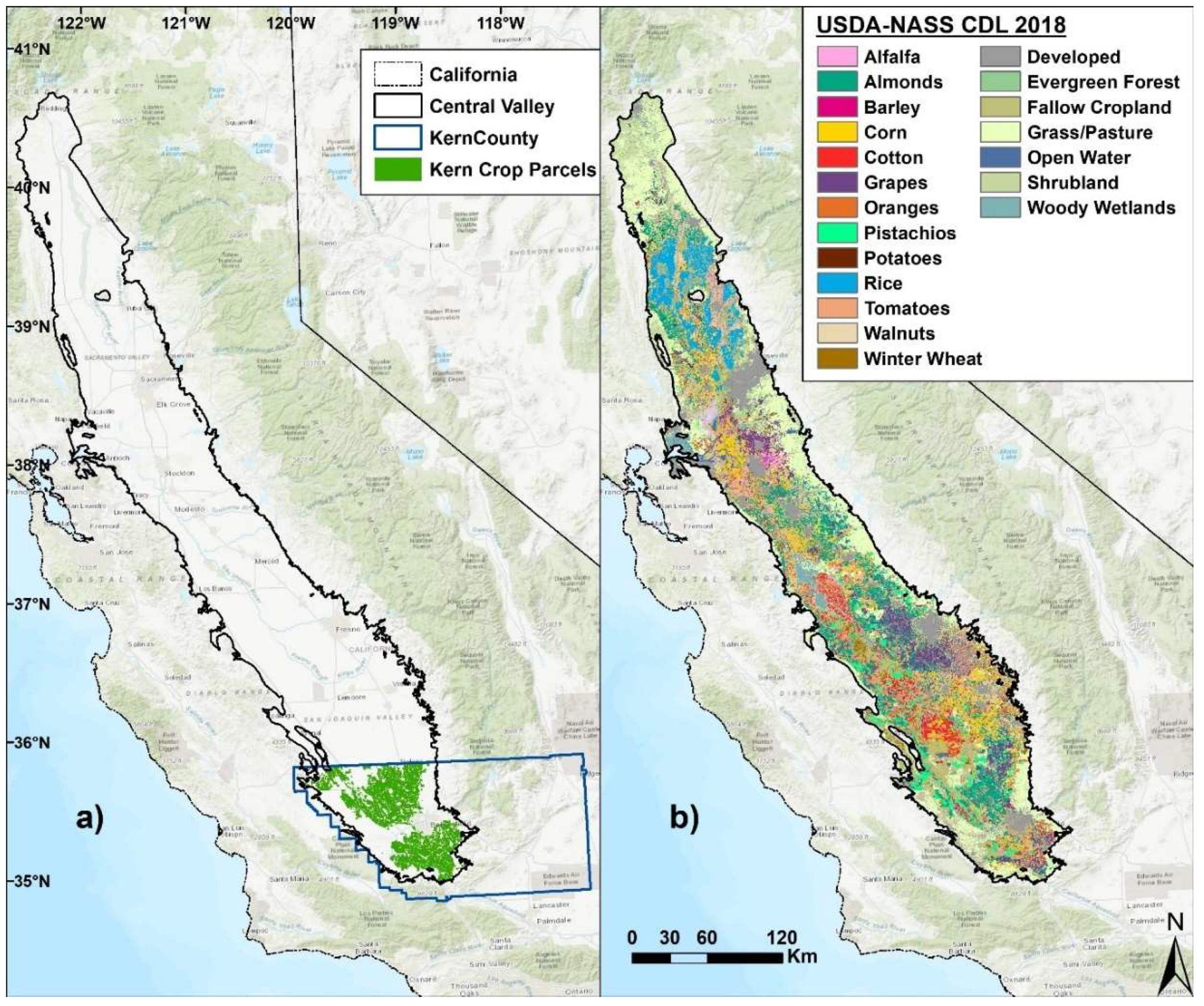
The Central Valley, as shown in Figure 1a, is a large flat valley that covers over 52,000 km2 and dominates the central portion of California extending nearly 720 km along a northwest–southeast axis [15,16]. The Central Valley is composed of the Sacramento Valley in the north, the San Joaquin Valley in the center, and the semi-arid Tulare Basin at the southernmost end [16]. The Central Valley is bordered by the Shasta National Forest on the north, the coastal range including major coastal cities to the west, the Sierra Nevada Mountains to the east (which provide much of the surface water), and the Mojave Desert to the southeast. The Central Valley has a Mediterranean climate especially in the southern part with hot, dry summers and mild, wet winters with most of the precipitation falling between November and March [17]. Kern County comprises the southernmost section of the Central Valley and includes the city of Bakersfield. The county is bordered by the Greenhorn Mountains to the northeast, the Antelope Valley to the southeast, and the Temblor Range in the west. Agricultural commodities in Kern County were valued at over $7.25 billion in 2017 [18].
We estimated crop water use for these areas by combining SSEBop ETa annual estimates with crop classifications. The crop classification grid is at the same 30-m resolution and is created by the USDA-NASS which provides annual grids from 2008 to 2018 [19]. The most recent USDA-NASS CDL for 2018 is shown in Figure 1b.
2.2. Landsat
This study utilized Google Earth Engine (GEE) cloud-based processing and the SSEBop approach on Landsat remote-sensing imagery to calculate annual actual evapotranspiration at 30-m resolution. GEE was used to generate annual ETa estimates for the entire Central Valley for the years 2008–2018, as well as for the last 20 years (1999–2018) for Kern County. For the annual Central Valley ETa, all Landsat Collection 1 Top-of-Atmosphere imagery from 13 Path/Rows (Path 41 Rows 35–36, Paths 42 Rows 34–36, Paths 43 Rows 33–35, Paths 44 Rows 32–34, and Path 45 Rows 32–33) was collected, totaling 4843 Landsat scenes, and processed. This imagery includes 839 Landsat 5 scenes (17%), 2602 Landsat 7 scenes (54%), and 1402 Landsat 8 scenes (29%) with an average of 430 images for each year or 33 images for each Path/Row. This number exceeds the suggested minimum of 10–12 images per year for each Path/Row recommended to generate a reliable remote sensing-derived ETa estimate [20].
Due to the heavy computer resource and processing requirements for ingesting millions of Landsat pixels for the entire Central Valley for multiple years, the SSEBop model has been implemented in the Google Earth Engine processing environment, which provides large-scale processing of thousands of Landsat images [21]. Processing that would normally take weeks or months can now be done in a matter of days. All Landsat pixels containing the Central Valley were processed in GEE using the SSEBop model as well as new cloud-based interpolation and aggregation algorithms for all scenes with 60% cloud cover or less. This includes masking clouds using the Landsat Quality Assessment band and Landsat 7 scan-line errors and filling these pixels through linear interpolation from contemporaneous scenes (within 48 days before/after an image) [22].
2.3. The SSEBop Modeling Approach
The Operational Simplified Surface Energy Balance (SSEBop) model is a thermal remote sensing method that ingests Landsat imagery and generates daily total actual evapotranspiration (ETa) [6]. The primary product of the method is the ET fraction, driven by land surface temperature (Ts) from the Landsat thermal band, which takes a fractional amount of alfalfa-reference potential ET (ETr) derived from GridMET to create actual ET [5,6,23]. GridMET is a gridded dataset at 4-km resolution provided by the University of Idaho that provides daily weather variables for the continental United States from 1979 to present [23]. SSEBop ETa is driven by the thermal band from Landsat 5/7/8 satellites, which is processed at the native spatial resolution—Landsat 5 (120 m), Landsat 7 (60 m), Landsat 8 (100 m)—but then resampled to 30 m. This method is described in detail in Senay [6]. SSEBop actual ET can be summarized with the following equation:
where ETa is actual ET (mm); ETr is alfalfa-reference (maximum potential) ET (mm) from GridMET which represents the maximum amount of daily water use under optimal water supply conditions; Ts is the land surface temperature derived from the Landsat thermal band (K); Tc is the cold/wet limit, derived from gridded maximum air temperature (K) representing the surface temperature at which maximum evapotranspiration is occurring; and is a surface psychrometric constant (K) [6]. The GridMET ETr has been bias-corrected with a coefficient of 0.85 derived from a comparison with California Irrigation Management Information System (CIMIS) station data (https://cimis.water.ca.gov/).
Similar to Senay, et al. [22], before ETa was computed for each scene, cloud-masked pixels were filled using per-pixel linear interpolation from images 48 days before and after the scene date. Daily ETa was calculated using Equation (1) in GEE along with daily GridMET ETr and then aggregated to the annual total.
The relative accuracy of SSEBop ETa has been evaluated multiple times and shown to match well with Ameriflux eddy-covariance flux towers as well as Max Planck Institute monthly ETa, demonstrating that SSEBop can detect spatial variability and monthly and annual trends with reasonable accuracy [20,22,24,25,26,27]. In Senay, et al. [5], we compared monthly SSEBop ETa to monthly MPI ETa from 1984 to 2011 for eight HUC-8 sub-basins in the middle and lower Central Valley and found an average r2 of 0.76 and average root mean square error (RMSE) of 11.7 mm. More recently, we compared monthly SSEBop ETa to Ameriflux eddy-covariance flux tower monthly ETa in the Upper Rio Grande Basin for non-cropland environments such as forest, shrubland, and grassland sites from 2007 to 2014 and found an average r2 of 0.85 and average normalized RMSE of less than 10% [22].
2.4. USDA-NASS Cropland Data Layer (CDL)
The USDA-NASS provides cropland data layers (CDL) for the United States from 2008 to present, which includes spatially explicit land use and land cover classification at 30-m resolution [19]. The CDL is released each year and is meant to represent crop-specific land cover—classifications for over 100 individual crop types—from the previous year’s growing season [28]. The CDL is primarily derived from Landsat 5, 7, and 8 imagery as well as other remote sensing datasets such as Deimos-1 imagery and the National Land Cover Database (NLCD) in a decision-tree classification algorithm [28,29]. The CDL originally provided 30-m resolution data from 2010, whereas 2008/2009 data were provided in coarser resolution; however, recently, USDA-NASS reprocessed 2008/2009 CDL to match the spatial resolution of the other CDL datasets from 2010 onwards [19]. The accuracy reported by USDA-NASS for the large-area crops ranges from 85 to 95% [29].
The CDL is the best crop-specific gridded dataset available for the entire Central Valley Lark, et al. [28], in a review of the use of USDA-NASS CDL in scientific publications, noted several potential biases and recommendations, which we included in this study as detailed in Section 2.5. For this study, only the 10 most expansive crops (in total area) between 2008 and 2018 for the Central Valley were utilized to summarize ETa. These 10 crops (alfalfa, almonds, corn, cotton, grapes, oranges, pistachios, rice, walnuts, and winter wheat) were selected from the larger dataset and other CDL classes were discarded. The top 10 crops in the Central Valley comprise about 17,000 km2 or roughly 33% of the valley area. Misidentified pixels are widely dispersed and isolated in marginal areas, so they were removed for the major CDL crops through a generalization procedure to retain only pixel clusters of 8 or more neighboring pixels. This resulted in a cleaner classification grid that more closely aligns with visual crop fields with minimal reduction in total crop area.
2.5. County Crop Acreage Reports
To estimate the area for the major crops in the entire Central Valley using the generalized CDL, we estimated area using the pixel-counting method but then bias-corrected based on a comparison with the county-reported annual crop reports provided by each individual county’s Agricultural Commissioner. The reported area from each California county was collected from the local Agricultural Commissioner’s annual reports for each major crop similar to the method used in Fulton, et al. [30]; annual county crop reports are publicly available through the California Department of Food and Agriculture (https://www.cdfa.ca.gov/exec/county/CountyCropReports.html).
The county crop areas were then aggregated up to the scale of the entire Central Valley and compared to the area estimates from the annual generalized USDA-NASS CDL. On average, the generalized CDL overestimated crop area by 4% or 6100 ha for all 10 crops. The average bias was determined at the scale of the entire Central Valley for each major crop by comparing the generalized CDL area against the aggregated county reported numbers from 2008 to 2017 (the 2018 acreage reports were not yet available at the time of this writing) and is included in Table 1. Crops such as almonds, cotton, rice, and walnuts were all estimated by the CDL to within 5% of the county crop reports.
The generalized CDL area for the entire Central Valley, including for 2018, for each major crop was then bias corrected using the 2008–2017 average bias of each crop type displayed in Table 1. This resulted in area estimates that were closer to the aggregated county-reported area in both magnitude (within +/− 1%) and annual variation (average ’r’ correlation value of 0.79) for all major crops, especially in alfalfa, almonds, cotton, rice, and walnuts. Overall, the bias correction of the generalized CDL acreage estimates provided a much more accurate reading based on county acreage reports. Estimating the area accurately was crucial in determining the volume of water use for each crop as part of this study; the water use estimates are dependent on not just the accuracy of the ET model but also heavily impacted by the area count utilized.
2.6. Kern County Crop Boundaries
The Kern County Department of Agriculture and Measurement Standards provides digitized annual crop parcel boundaries for all of Kern County from 1997 to the present (http://www.kernag.com/gis/gis-data.asp) as used in Shivers, et al. [13]. The crop parcel boundaries provide county-scale crop type classification for Kern County with a wider temporal extent (1999–2018) as well as more accurate area estimates than the estimated CDL area, and cleaner crop sampling zones for ETa sampling. For the analysis of Kern County crop water use from 1999 to 2018, the area counts reported in each parcel boundary were collected, aggregated, and used to create volumetric water use from SSEBop ETa without any bias correction on the area, as was done with the USDA-NASS CDL, but instead were assumed to be accurate counts. The crop parcel boundaries were an invaluable dataset to this study as an expansion on the crop data information provided by USDA-NASS. Not only does this dataset provide a longer time-series of crop type information dating back to 1999, it also provides more accurate area estimates for each parcel. When compared to the generalized CDL area counts for the matching crops in Kern County, the CDL accurately identifies 87% of the crop parcels produced by Kern County—underestimating the crop area by 13%.
Many of the parcels that the CDL failed to identify had low Normalized Difference Vegetation Index (NDVI) values suggesting that these parcels may not have been actively farmed in that year. Because we considered only “active crop parcels”, the Kern County crop parcels were filtered in each year for parcels that averaged ≥ 0.5 in May–September maximum NDVI, and so, only these parcels were included for further analysis. Water use was determined using the area provided with the crop parcel dataset for those parcels that were “active”. To maintain consistency with the CDL summaries for the entire Central Valley, the SSEBop ETa was averaged for each crop type and converted into volumetric water use estimate for each year using the corresponding crop area.
2.7. Other Datasets
Other remote sensing datasets utilized included gridded annual total precipitation for the Central Valley for the 1999–2018 period extracted from 4-km PRISM (Parameter-elevation Regressions on Independent Slopes Model) precipitation datasets in order to calculate net irrigation [31].
Additionally, maximum NDVI was derived from Landsat to determine the “active” crop parcels in Kern County crop boundaries described in the previous section. The May–September maximum Landsat surface reflectance NDVI was created in GEE for the period of 1999–2018. The May–September seasonal maximum was chosen to identify crop boundaries that were actively vegetated in the peak growing season while not being rainfed. According to PRISM, the May–September period has the lowest precipitation totals for the valley in the 1999–2018 period annually ranging from 3–55 mm and averaging 18 mm as opposed to the April–October period which annually ranges from 90–500 mm and averages 315 mm.
The shapefile of the Central Valley was acquired from the U.S. Geological Survey’s Central Valley Hydrologic Model, which provides the digital extent of the alluvial deposits of the contiguous Sacramento, San Joaquin, and Tulare Lake groundwater basins and encompasses an approximate 50,000 km2 area of central California [16].
2.8. Water Use Estimates and Net Irrigation
To calculate crop water use in volumetric units, the spatially-averaged SSEBop annual ETa (mm) was determined for each crop type at each scale of analysis and then converted into hectare-meters (ha-m) using the corresponding crop area as follows:
where Crop Water Use (ha-m) is the volume of water used by a specific crop in a given year, ETa (m) is the spatially averaged SSEBop ETa for a given crop, and Crop Area (ha) is the surface area of the crop.
One ha-m is equal to 10,000 m3 (8.11 ac-ft). For net irrigation, the annual precipitation is subtracted from the annual ETa. It is important to note that assuming all precipitation is effective may underestimate the net irrigation amount.
2.9. Trend Analysis
For the time-series analysis of crop ETa, the simple Mann–Kendall (MK) trend test was used to test the presence or absence of statistically significant trends in water use at both the county and valley scale as well as the scale of individual pixels. The MK test is a non-parametric rank-based method for identifying monotonic trends and is widely used in time-series analysis of hydrologic data [32,33,34,35]. This test examines the slopes between pairwise samples ranked chronologically and results in an overall MK score that indicates a positive or negative trend along with 95% confidence level (p-value < 0.05) [33,35]. We tested for serial correlation in the sample with the Durbin–Watson statistic (not shown) prior to running the MK test and we found that there was no serial correlation in the statistically significant results. The Theil–Sen estimator was then used to measure the magnitude of the slope over the study period. The Theil–Sen estimator is a non-parametric alternative to the parametric ordinary least squares regression line and is frequently used alongside the Mann–Kendall test in hydrologic time-series analysis [35,36].
One limitation of the MK test is that it requires a minimum of 8–10 data samples to provide a statistically significant result. There are 11 years’ worth of USDA-NASS CDL (2008–2018) and therefore a maximum of 11 annual crop ETa data points which meets the minimum requirement of the test; however, low sample size may affect the ability to detect statistically significant trends in some crops. The MK test was utilized to detect trends in SSEBop ET summarized by USDA-NASS CDL as well as water use characterized by the Kern County crop boundaries from 1999 to 2018. Additionally, the MK test was conducted on a per-pixel basis for all SSEBop annual ETa in Kern County for 1999–2018. The per-pixel MK uses the same statistical process and produces the same resulting MK statistic, Theil–Sen slope, and p-value, but conducts the test for each pixel in the time-series stack of annual grids. The results of this 20-year “trend grid” were then contextualized in the discussion on individual fields within Kern County and how the shifting crop types of those fields affected trends in water use over time.
3. Results
3.1. Crop Water Use in the Central Valley 2008–2018
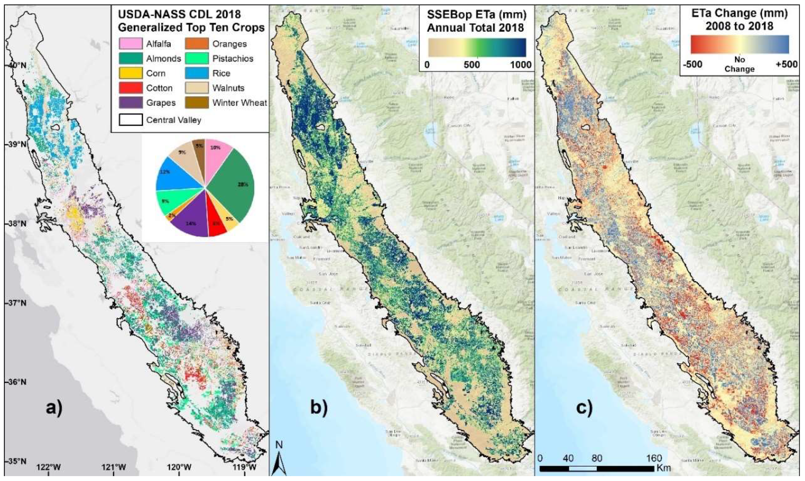
The top 10 major crops for the entire Central Valley, in area, are alfalfa, almonds, corn, cotton, grapes, oranges, pistachios, rice, walnuts, and winter wheat. Figure 2a displays the geographic spread and relative distribution of these 10 crops for the year 2018, the most recent year that the CDL data is available at the time of writing. Although the total area of these top 10 crops stays relatively stable over the 2008–2018 period at about 1.6 million ha, the distribution of the crops shifts over time. While crops such as cotton or rice stayed relatively stable over this period, other crops such as alfalfa and winter wheat declined in area while nut crops such as almonds, pistachios, and walnuts increased. These shifts in preferred crops greatly influenced the water use patterns in the Central Valley.
SSEBop ETa, such as the 2018 annual total shown in Figure 2b, can show a bird’s eye view of the spatial variability and relative water use across the entire valley, and crop type information provides valuable context to understand these patterns. For instance, the rice fields identified in the CDL, which are frequently flood-irrigated, are detected in the 2018 SSEBop ETa as dark blue signifying 1000 mm or more of ETa in a given year. The ETa change map in Figure 2c shows bright blue in these same fields indicating a positive change of up to 500 mm in 2018 as opposed to 2008, but as shown later in the Mann–Kendall trend results, the trend in rice overall decreases. These ETa change maps are useful but sampling and charting the entire time-series provides more detail than we would otherwise see.
Table 2 presents the averages for the final bias-corrected crop area estimates as well as the difference between the last year (2018) and the first year (2008) for the top 10 major crops. The area estimates demonstrate a substantial decline in alfalfa and winter wheat and substantial increases in nut crops such as almonds, pistachios, and walnuts from the first year of the study in 2008 to the last year in 2018. Almonds are distributed throughout the valley and do not seem to decrease during the 2012–2016 drought. In fact, almonds show an increase of 30% in 2018 as compared to 2008. Other crops that see an increase in area are grapes, pistachios, and walnuts while alfalfa, corn, oranges, and winter wheat all see decreases in 2018 as opposed to 2008, which changes their overall water use totals.
Trend analysis, using the MK test, reveals the crops that show statistically significant increases or decreases in crop area and the results are displayed in Table 3 for the 10 major crops. The results highlight that almonds, grapes, pistachios and walnuts all have statistically significant increasing trends over the 2008–2018 period whereas alfalfa and winter wheat have statistically significant decreasing trends. This analysis confirms that almonds and other fruit and nut crops are increasing in crop area over time in the Central Valley while more traditional row crops such as alfalfa are seeing declines in crop area over the same period. The remaining crops did not show a significant trend although it can be inferred from the slope that corn, cotton, and rice decreased in area over the 11-year period.
These shifting patterns in crop area impact the overall water use for the major crop types. Figure 3 shows the ETa, crop area (ha), water use (ha-m), and net irrigation (ha-m) after removing all precipitation for five of the top 10 crops in the valley. The annual variation of ETa is small in comparison to crop area which has a large impact on overall water use. The total annual crop water use for the top 10 crops in the Central Valley averages over 1.19 million ha-m. The primary water users in 2008 are alfalfa, almonds, and rice, which each consume around 20% of the total crop water use for the valley’s major crops. By 2018, that share of crop water use shifts and alfalfa is only 9% of the total water use while almonds increase to 33% (see Table 4). Rice and winter wheat see more modest declines in their share of water use while pistachios and walnuts see modest increases. The remaining crops show minimal or no real change in the proportion of total water use shifting +/− 4% of the total from 2008 to 2018. However, the difference in each crop’s water use from the first year of the study in 2008 and the last year in 2018 displays some dramatic shifts as indicated in Table 4. Alfalfa, corn, oranges, rice, and winter wheat all declined in 2018 as compared to 2008 whereas almonds, pistachios, and walnuts saw dramatic increases. Cotton and grapes also saw increases but much more modest. Pistachios showed the most dramatic change with a 115% increase in 2018 as compared to 2008 although the total share of crop water use was still less than 10%. Alfalfa saw the most dramatic decline both in the percentage drop but also in magnitude and the share of total crop water use. In 2008, alfalfa used 238,316 ha-m of water but 11 years later, the crop used less than 100,000 ha-m, a 58% decline. Table 4 also displays the mean crop water use for the 2012–2016 California drought as well as the percent decline from the 2008–2018 mean. Almost all 10 crops saw a decline in mean water use during the drought, with the exceptions of almonds (7% above the mean) and grapes (8% above the mean). Even under regional drought conditions, almonds still averaged 364,074 ha-m of water use per year. These results demonstrate that almonds continue to be productive in the Central Valley even in drought conditions.
The MK trend analysis on crop water use, displayed in Table 5, corroborates the shifting trends in Central Valley crop water use. Alfalfa and almonds have an inverse pattern to one another with alfalfa showing a statistically significant declining trend in crop water use over the 2008–2018 period at a rate of 13,901 ha-m per year. Conversely, almonds show a statistically significant increase in crop water use at a rate of 13,488 ha-m per year. Other crops that have statistically significant increasing trends are grapes and walnuts. On the other hand, crops such as rice and winter wheat show statistically significant decreasing trends. Similar to the crop area, traditional row crops are declining in water use over the 11-year period while fruit and nut crops are increasing in water use over the same period. While the SSEBop ETa values taken independently provide a useful relative measure of water use in the Central Valley, when contextualized and summarized by crop type, remote sensing can provide easily interpretable and vital metrics for the consumption of water by major agricultural crops.
3.2. County-Scale Crop Water Use—Kern County, 1999–2018
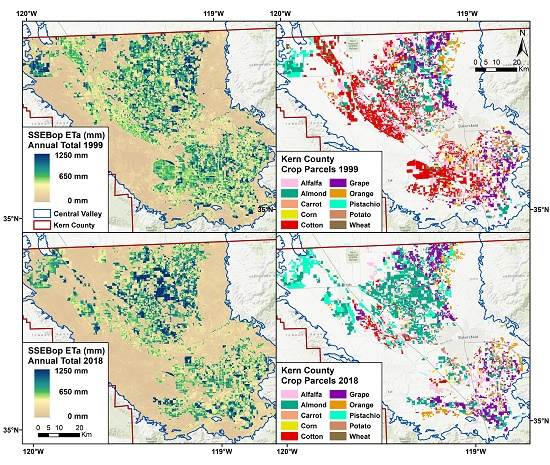
This same analysis was conducted on the scale of an individual county that has cropland in the Central Valley to evaluate the county-scale change in crop water use. For the county-scale analysis, we used the crop parcel shapefiles provided by Kern County from 1999 to 2018 to analyze 20 years of crop water use in Kern County rather than rely on the generalized USDA-NASS CDL, which is available only from 2008 to present. Figure 4 displays the SSEBop ETa and crop classifications for Kern County in the southernmost part of the Central Valley for the year 1999 and the year 2018. Total SSEBop ETa does not show a clear increasing or decreasing trend in Kern County from 1999 to 2018 yet there are clear shifts in the distribution of ETa across the county over time.
The top 10 crops for Kern County and their crop area are displayed in Table 6. The active crop parcels in Kern County average over 205,000 ha from 1999 to 2018 but there is a consistent decline over the 20-year period at a rate of 1000 ha per year. Most of these “lost” parcels seem to occur south of the city of Bakersfield where cotton and alfalfa fields predominated in the year 1999, as shown in Figure 4b. Overall, cotton seems to decline in favor of almonds from 1999 to 2018 in Figure 4. In 1999, cotton in Kern County had a production value of $233 million, according to county crop reports, but by 2017, the production value of cotton fell to $74 million [18]. Almonds, on the other hand, increased in value from $143 million in 1999 up to $1.26 billion by 2017 [18].
Indeed, in the share of the total crop area for the top 10 crops, cotton occupies 32% of the active crop parcels in 1999 but by 2018, cotton occupies 4% of the crop area. alfalfa shows a crop area decline of 8%. Almonds, on the other hand, nearly triple in the share of total crop area up to 38% by 2018. The change in crop area shows a consistent decline in traditional crops such as alfalfa, carrots, corn, cotton, potatoes, and wheat while shifting towards investment in nut crops such as almonds and pistachios. Even during severe drought conditions, such as 2012–2016, fruit and nut crops show an appreciable increase in crop area, compared to the 20-year mean, whereas more traditional crops see substantial declines, such as a 60% decrease in crop area for cotton and a 40% decline for wheat.
Trend analysis using the MK test on the crop area (as shown in Table 7) confirms the declining trends in traditional crops in favor of fruit/nut crop types. Cotton shows the sharpest decline with a statistically significant decrease at a rate of 3589 ha/year. Alfalfa and wheat also see significant, if smaller, declines in crop area. Smaller crops such as carrots, corn, and potatoes also see statistically significant decreasing trends in crop area at a rate between 100 and 200 ha/year. However, the fruit/nut crops all see statistically significant increasing trends over the 20-year period. Almonds increase in area at a rate of 2465 ha/year and pistachios increase at a rate of 1095 ha/year. Although the total footprint of pistachios is smaller than that of almonds, their increasing importance in Kern County’s agricultural production is clear. Grapes and oranges also see statistically significant increases in crop area over time, although to a smaller extent than nuts.
On average, the top 10 crops of Kern County consume 158,312 ha-m of water annually from 1999 to 2018. In the beginning of the study period, cotton is the predominant water user in the county consuming 26% or 41,075 ha-m of water in 1999 but, as shown in Figure 5, as the crop area for cotton declines, the water use also declines until cotton is reduced to only 3% of the total crop water use in 2018 at less than 4000 ha-m. The decline in crop water use is directly correlated with the decline in crop area with an r2 = 0.99. Alfalfa, the second highest consumer of water in 1999, saw a similar reduction in crop water use as its agricultural footprint receded. Alfalfa consumed 32,015 ha-m of water in 1999, 20% of the total crop water use. However, by 2018, alfalfa was reduced to just over one-third of that volume (11,095 ha-m) and consumed just over 8% of the total crop water use. Other row crops such as wheat also experienced a 5% decline in their share of total crop water use. The 2018 water use for wheat was 86% less than the water used in 1999. Water use by these three traditional row crops was further reduced during the 2012–2016 California drought. Alfalfa fared the best at only 14% below the 20-year mean during the drought, but cotton and wheat saw drought reductions of 61% and 38%, respectively.
As for the fruit/nut crops in Kern County, almonds unsurprisingly become the heaviest water user in Kern County as the agricultural footprint of almond production expanded. Eighteen percent of total crop water use in 1999 was consumed by almonds at 29,275 ha-m but by 2018, the total share of crop water use rose to 48% or 66,243 ha-m. This increase in crop water use is directly linked to the rise in crop area as the annual area and annual water use for almonds are correlated with an r2 = 0.97. Pistachios saw a similar pattern as pistachios increased 164% in 2018 from the 1999 total water use. This shifts the proportion of crop water use for pistachios from 4% in 1999 up to 13% in 2018. Fruit crops such as grapes showed a more stable pattern over the 20-year period. Although grapes saw an increase in water use from 1999 to 2018, the increase was more subtle with only a 23% increase in 2018 totals as compared to 2008 with the proportion of total water use shifting 5% during the 20-year period. Oranges showed a similar pattern but even more subtle (see Table 8). Furthermore, unlike the traditional row crops, none of the fruit/nut crops showed a decline in water use during the 2012–2016 drought, but instead saw percent deviations that were increased from the 20-year mean.
The MK trend results presented in Table 9 confirm these crop water use patterns. The traditional row crops such as alfalfa, cotton, potatoes, and wheat all show statistically significant declining trends in crop water use over the 1999–2018 period. Cotton has the sharpest decline in crop water use—a total rate of change for the 20-year period of 42,140 ha-m. Alfalfa and wheat have smaller declining rates of water use. Whereas the traditional row crops all experience statistically significant declining trends in crop water use over the 20-year period, the fruit and nut crops all have statistically significant increasing trends in water use. Almonds have the most pronounced increase, which equates to an overall 20-year rate of change of 60,700 ha-m. The trend for pistachios is less extreme but increases as well at a rate of 744 ha-m/year. Grapes and oranges also show strong increasing trends but are more subtle than the nut crops.
3.3. Field-Scale Analysis and Pixel-Based Mann–Kendall Trends
Mapping crop ET on the scale of the entire Central Valley or on the scale of an entire county can provide a broad view of water use by different crops, but the true advantage of Landsat-derived ET with similar resolution crop classification is the analysis of trends at the scale of individual fields. Here, we created per-pixel trend statistic grids by stacking all annual SSEBop ETa grids for Kern County from 1999 to 2018 and then running the Mann–Kendall trend test on each pixel stack rather than crop totals. Figure 6 displays the 20-year (1999–2018) mean SSEBop ETa for all of Kern County as well as the Theil–Sen slope pixels which showed statistically significant Mann–Kendall trends (increasing/decreasing). A cursory analysis of the per-pixel trend datasets using the Kern County 2018 crop parcels demonstrates an overall increasing trend for statistically significant pixels in agricultural parcels that may be linked to the statistically significant positive trends in almonds and pistachios, as outlined in the previous section. The 2018 fields, which are identified as almonds, show a trend toward increasing slope in ETa. Conversely, the 2018 parcels identified as wheat, show a statistically significant decrease which would suggest that these fields are trending downward to less water use over time. These pixel trends can also help identify individual fields that are increasing or decreasing over time and allow more in-depth analysis of crop water use, which takes full advantage of higher-resolution Landsat ET.
Figure 7 displays eight crop parcels that showed an equal mix of declining and increasing trends in the Mann–Kendall trend test. The statistically significant Theil–Sen slope pixels displayed in Figure 7 are only those that had a p-value < 0.05 (95% confidence) for each pixel. All eight of these crop parcels were identified by the Kern County Department of Agriculture and Measurement Standards as being cotton fields in the year 1999, the first year of the study. These fields are in the western section of the county just south of Lost Hills, California in an area that was predominantly cotton in the early 2000s but transitioned into almond and pistachio production by 2010. Each of these fields is approximately 60 ha in size with 4 of the fields (# 1–4) showing predominantly statistically significant declining trends in ET and the other 4 fields (# 5–8) showing predominantly significant increasing trends. Figure 7 also displays the spatially integrated magnitude of water use for each of the fields which is distributed across the 60-ha area.
The crop type identification for each of these fields provides the context to understand these patterns and explain the trends in the pixel-based MK grids. The water use for each of the eight fields is shown in Figure 7, all of which are designated as cotton fields in 1999. We also determined the May–September maximum NDVI for each of these fields in addition to the water use. From 1999 to 2005, fields 1–4 had an average high NDVI ranging from 0.73–0.79 and water use at an average of 37 ha-m, which signifies active cotton production. In every year after 2007, the NDVI for each of these fields fell below 0.2. However, starting in 2007, NDVI fell below 0.2 and the mean water use for all four fields between 2007 and 2018 averaged only 3 ha-m, not accounting for precipitation, which suggests that these fields fell out of active use. Fields 5–8 follow a different pattern, transitioning from individual cotton fields in the 1999–2005 period to almond production in the period 2005–2018. Fields 5–8 had an average high NDVI of approximately 0.75 in the period 1999–2001 and in 2004 but low NDVI in the period 2002–2003 and from 2005 to 2007, suggesting that irrigation did not take place every year. The mean water use during the years of low NDVI was approximately 2 ha-m, without accounting for precipitation, suggesting no active use. It is important to keep in mind that this is a spatially integrated estimate for the entire 60 ha where 2 ha-m is distributed across the area.
Starting in 2007, NDVI and water use gradually increased, but water use remained low at an average of 18 ha-m through 2009, perhaps because the almond crops had not yet reached maturity. The almond fields appear to have reached full maturity in 2011 when the fields average 0.64 maximum NDVI and 51 ha-m of water. From 2012 to 2018, all four fields averaged 59 ha-m of water use, suggesting active almond production. Field 6 was the lowest, perhaps due to roads and more bare areas, which can be seen in Figure 7a,b. This example of the changing trends in eight former cotton fields exemplifies the advantages of using actual evapotranspiration at Landsat-scale resolution along with high resolution crop classification to examine field-scale changes in water use over time.
4. Discussion
This application of SSEBop ETa provides a long-term study of irrigation and evapotranspiration for the entire Central Valley. Many previous studies of crop water use in the Central Valley are site-specific studies of limited spatial and temporal extent [12,14]. Other studies use crop coefficients for generic (e.g., cereal) or specific (e.g., corn) vegetation types which assume optimal practices in irrigation scheduling and availability of water [11]. However, direct observation of ETa using a simplified remote sensing model such as SSEBop can capture Central Valley water use at a large spatial and temporal extent without assuming ideal crop type coefficients or the level of irrigation efficiency. These gridded ETa estimates can provide a broad view of the spatial variability and distribution of vegetative water use. However, crop type classification, such as USDA-NASS CDL, provides the context to transform gridded ETa into useful information on how much water different crops utilize and how that crop water use changes over time. Results from this study indicated that while the 1.2 million ha-m utilized annually by the 10 major crops in the Central Valley from 2008 to 2018 remains stable even during drought periods, the distribution of that water use shifts from traditional row crops such as alfalfa and cotton to nut and fruit crops. While alfalfa and cotton decline during dry years such as the 2012–2016 drought, fruit and nut crops such as almonds and pistachios increase in crop area and associated water use. Alfalfa declines nearly 60% from 2008 to 2018 and over 100,000 ha of alfalfa transition to different crop types by the year 2018, primarily almonds and pistachios. The observed strong relationship between crop water use and area indicates the reliability of these methods to estimate both ETa and crop area. For the same crop type, it is apparent that increased water use comes mainly from increased area as the annual variation in ET is expected to remain low under optimal irrigation conditions.
The patterns observed in this study of crop types shifting from traditional row crops such as alfalfa and cotton in favor of more permanent tree crops such as almonds or pistachios mirrors results reported in Faunt, et al. [7]. Faunt, et al. [7] found that, since 2000, field/row crops were being replaced by permanent orchards and vineyards which has led to ’demand hardening’ of irrigation water demands as the land cannot be easily fallowed. This was linked to a reduction in groundwater storage as the prolonged drought conditions reduced surface water availability which exacerbated groundwater extraction [7]. Although this study did not include a groundwater component or full water budget analysis, the patterns found in this study align closely with Faunt, et al. [7] and the higher resilience of crop water use for crops such as almonds during the 2012–2016 drought, as found in this study, may be contributing to increased groundwater extraction.
Almonds and pistachios are two high-value crops that have a reputation of being drought tolerant [37]. Previous studies have suggested that California needs 173,000 ha-m annually for almond and pistachio production [37]. The results of this study show the actual water use of almonds and pistachios to be closer to an annual average of 380,000 ha-m in raw water use and 250,000 ha-m in net irrigation once precipitation has been removed. As Fulton, et al. [30] point out, the California almond industry is an important and growing sector of the state’s economy with an economic value accounting for 25% or approximately $5.1 billion of California’s 2015 farm exports. Fulton, et al. [30] found that the water footprint of almonds varied by different sections of the Central Valley and almond yields were higher in the southern part of the valley, which is associated with a hotter climate and therefore had a lower overall water footprint. It has been commonly reported that it takes 4.16 L of water (the English unit of 1.1 gallons is the commonly cited metric in grey literature) to produce a single almond nut [38]. To test this idea, we calculated the volume of water/nut rate for each year of this study based on the bias-corrected CDL area and the volume of water use from the entire Central Valley. Using the average production of shelled almonds per unit of area from the USDA-NASS 2012 Census of Agriculture and the volume of water measured by this study, we found that the ratio of water per almond nut to average closer to 3.56 L (0.94 gallon) per almond—SSEBop water use falls within 15% below the commonly reported metric [39]. The fact that the SSEBop water use aligns so closely with the commonly reported field-scale measurement reinforces the reliability of a remote sensing method such as SSEBop to quantify water use at the field scale.
Determining and bias-correcting acreage from USDA-NASS CDL is not without its challenges and has a substantial impact on the final water use estimates but does provide a crucial view of changing crop types and their effect on irrigated consumptive water use. The primary limitation to this study is the limited temporal extent. Crop classification data, created with consistent methods, is only available for the entire Central Valley from 2008 to present from USDA-NASS [19]. Although Senay, et al. [5] demonstrated that SSEBop ETa can be reliably estimated for large spatial extents for the entire Landsat archive of thermal sensors back to 1984, without accompanying crop classification data, the mapping of crop water use is limited to recent time periods. The crop parcel shapefiles provided by Kern County provide an invaluable asset to mapping crop water use for a longer period, dating back to 1999, but are limited to the boundaries of the county; similar shapefiles for other counties in the Central Valley are not currently publicly available. SSEBop ETa can be measured with Landsat for any area of the world at 30-m resolution but contextualizing and summarizing the gridded ET estimates relies on high-resolution crop type parcels. In the future, if other counties or states provide similar data to Kern County going back 20 or 30 years, a more expansive study like this one can be completed at multiple spatial scales.
5. Conclusions
This study characterizes crop water use for the entire Central Valley, one of the most productive agricultural regions in the United States, from 2008 to 2018 at 30-m resolution. The drought periods that have affected California in recent years have limited water resources, depleted surface water, and exacerbated groundwater extraction. Therefore, understanding the consumptive water use by different crop types is essential for sustainable water management and irrigation efficiency. In this study, we evaluated crop water use at three spatial scales—the entire Central Valley from 2008 to 2018 using USDA-NASS CDL crop classification, the scale of an individual county using Kern County crop parcels from 1999 to 2018, and the scale of individual cotton fields that transitioned in crop type over the 1999–2018 period. Our primary objective was to characterize how crop water use changes with time at different scales, including the response to a drought period such as the 2012–2016 California drought. The 10 major crops in the Central Valley average 1.2 million ha-m of water use annually from 2008 to 2018 even during the drought, but the distribution of water use shifts to different crops over time. These results are consistent at every spatial scale evaluated in this study.
A primary result of this study is the reduction in water use from traditional row crops such as alfalfa and cotton and an increase in water use by fruit/nut tree crops such as almonds and pistachios, even during substantial drought periods. Much of this change in water use can be attributed to the changing area footprints of these crops. Alfalfa sees a dramatic decline in crop water use at every scale of analysis with a statistically significant decline in water use at a rate of 13,901 ha-m per year from 2008 to 2018 for the Central Valley. Almonds, on the other hand, show a significant increase in water use at the same scales, increasing at a rate of 13,488 ha-m per year. Where crops such as alfalfa, cotton, and winter wheat see reductions in water use during the 2012–2016 drought, crops such as almonds and pistachios either remain stable or increase during the same period. Cotton fields in Kern County exemplify this finding as the crop area and crop water use fluctuate and decline dramatically during drought periods in 2007–2009 and 2012–2016.
In Kern County, using a longer time-series of data and a different crop classification source, we found similar results: a significant decline in traditional row crops in favor of high-value nut crops. Cotton in Kern County shows a statistically significant decline at a rate of 3589 ha/year and 2107 ha-m of water per year from 1999 to 2018. Almonds in Kern County show a statistically significant increase at a rate of 2465 ha/year and 3035 ha-m/year for the same 20-year period. We also found individual fields in Kern County that transition from cotton production in the early 2000s to almond production in the latter half of the 2000s with the accompanying increase in crop water use at an average of over 55 ha-m for a 60-ha almond field. These patterns hold true at all scales of analysis in this study—the valley, the county, and the level of individual fields.
This study provides an application of gridded actual evapotranspiration (ETa) for the entire Central Valley to map water use using a remote sensing-derived crop classification dataset. Due to the difficulty in calculating ETa at a large spatial and temporal scale, this study is the first of its kind to characterize water use patterns in differing crop types for the entire Central Valley of California. This study once again demonstrates the importance of the historical Landsat archive as well as the robustness of the SSEBop ETa model to capture the spatiotemporal dynamics of water use. The 30-m resolution of Landsat-derived ETa and similar-resolution crop classification allows for field-scale analysis of shifting crop types and crop water use trends in California during some of the most severe drought periods. As crop classification improves and satellite coverage expands, this study can be extended to monthly or even daily fluctuations in crop water use or water use variability within individual fields. This information can also inform water managers as to increased efficiency in irrigation for high-value crop types. This study demonstrates the continued importance of thermal remote sensing satellites such as Landsat to the measurement and analysis of water resources. This same approach can be applied to any basin that has crop classification data available. Irrigation managers, water resource planners, and policy makers can utilize these powerful tools to better manage water resources.
Author Contributions
Conceptualization: M.S., G.B.S.; Methodology: G.B.S., M.S.; Software: M.S.; Validation: M.S.; Formal Analysis: M.S.; Investigation: M.S., G.B.S.; Data Curation: M.S.; Writing—Original Draft Preparation: M.S.; Writing: —Review and Editing: G.B.S., M.S.; Visualization: M.S.; Supervision: G.B.S.; Project Administration: G.B.S.; Funding Acquisition: G.B.S.
Funding
This work was performed under U.S. Geological Survey (USGS) contract G15PC00012 in support of the USGS Water Census program through the USGS Land Change Science funding mechanism.
Acknowledgments
We thank the reviewers, including USGS internal reviewer Stefanie Kagone, for their helpful comments and suggestions on this manuscript. This study is part of the U.S. Department of the Interior’s WaterSMART (Sustain and Manage America’s Resources for Tomorrow) program. All the data used in this study were obtained from public domains and are freely available. Any use of trade, firm, or product names is for descriptive purposes only and does not imply endorsement by the U.S. Government. Additional thanks is given to MacKenzie Friedrichs from the USGS EROS Center and collaborators from the Desert Research Institute for advice and assistance in utilizing Google Earth Engine to process the SSEBop model on Landsat imagery.
Conflicts of Interest
The authors declare no conflict of interest.
Data Availability
All original 2008–2018 annual total SSEBop ETa grids for the entire Central Valley, in addition to the Kern County 1999–2018 SSEBop annual total ETa, and the Kern County per-pixel Mann–Kendall trend, and Theil–Sen slope grids are publicly available as a U.S. Geological Survey data release in Schauer and Senay [40].
References
- Nelson, K.S.; Burchfield, E.K. Effects of the structure of water rights on agricultural production during drought: A spatiotemporal analysis of California’s central valley. Water Resour. Res. 2017, 53, 8293–8309. [Google Scholar] [CrossRef]
- Matios, E.; Burney, J. Ecosystem services mapping for sustainable agricultural water management in California’s central valley. Environ. Sci. Technol. 2017, 51, 2593–2601. [Google Scholar] [CrossRef] [PubMed]
- Pathak, T.B.; Maskey, M.L.; Dahlberg, J.A.; Kearns, F.; Bali, K.M.; Zaccaria, D. Climate change trends and impacts on California agriculture: A detailed review. Agronomy 2018, 8, 25. [Google Scholar] [CrossRef]
- Howes, D.J.; Fox, P.; Hutton, P.H. Evapotranspiration from natural vegetation in the central valley of California: Monthly grass reference-based vegetation coefficients and the dual crop coefficient approach. J. Hydrol. Eng. 2015, 20, 04015004. [Google Scholar] [CrossRef]
- Senay, G.B.; Schauer, M.; Friedrichs, M.; Velpuri, N.M.; Singh, R.K. Satellite-based water use dynamics using historical Landsat data (1984–2014) in the southwestern United States. Remote Sens. Environ. 2017, 202, 98–112. [Google Scholar] [CrossRef]
- Senay, G.B. Satellite psychrometric formulation of the operational simplified surface energy balance (Ssebop) model for quantifying and mapping evapotranspiration. Appl. Eng. Agric. 2018, 34, 555–566. [Google Scholar] [CrossRef]
- Faunt, C.C.; Sneed, M.; Traum, J.; Brandt, J.T. Water availability and land subsidence in the Central Valley, California, USA. Hydrogeol. J. 2015, 24, 675–684. [Google Scholar] [CrossRef] [Green Version]
- Xiao, M.; Koppa, A.; Mekonnen, Z.; Pagán, B.R.; Zhan, S.; Cao, Q.; Aierken, A.; Lee, H.; Lettenmaier, D.P. How much groundwater did California’s Central Valley lose during the 2012-2016 drought? Geophys. Res. Lett. 2017, 44, 4872–4879. [Google Scholar] [CrossRef]
- Thomas, B.F.; Famiglietti, J.S.; Landerer, F.W.; Wiese, D.N.; Molotch, N.P.; Argus, D.F. GRACE groundwater drought index: Evaluation of California central valley groundwater drought. Remote Sens. Environ. 2017, 198, 384–392. [Google Scholar] [CrossRef]
- Famiglietti, J.S.; Lo, M.; Ho, S.L.; Bethune, J.; Anderson, K.J.; Syed, T.H.; Swenson, S.C.; de Linage, C.R.; Rodell, M. Satellites measure recent rates of groundwater depletion in California’s Central Valley. Geophys. Res. Lett. 2011, 38, L03403. [Google Scholar] [CrossRef]
- Szilagyi, J.; Jozsa, J. Evapotranspiration trends (1979-2015) in the Central Valley of California, USA: Contrasting tendencies during 1981–2007. Water Resour. Res. 2018, 54, 5620–5635. [Google Scholar] [CrossRef]
- Semmens, K.A.; Anderson, M.C.; Kustas, W.P.; Gao, F.; Alfieri, J.G.; McKee, L.; Prueger, J.H.; Hain, C.R.; Cammalleri, C.; Yang, Y.; et al. Monitoring daily evapotranspiration over two California vineyards using Landsat 8 in a multi-sensor data fusion approach. Remote Sens. Environ. 2016, 185, 155–170. [Google Scholar] [CrossRef] [Green Version]
- Shivers, S.; Roberts, D.; McFadden, J.; Tague, C. Using imaging spectrometry to study changes in crop area in California’s Central Valley during drought. Remote Sens. 2018, 10, 1556. [Google Scholar] [CrossRef]
- Anderson, M.; Gao, F.; Knipper, K.; Hain, C.; Dulaney, W.; Baldocchi, D.; Eichelmann, E.; Hemes, K.; Yang, Y.; Medellin-Azuara, J.; et al. Field-scale assessment of land and water use change over the California delta using remote sensing. Remote Sens. 2018, 10, 889. [Google Scholar] [CrossRef]
- Prueger, J.H.; Parry, C.K.; Kustas, W.P.; Alfieri, J.G.; Alsina, M.M.; Nieto, H.; Wilson, T.G.; Hipps, L.E.; Anderson, M.C.; Hatfield, J.L.; et al. Crop water stress index of an irrigated vineyard in the Central Valley of California. Irrig. Sci. 2018, 37, 297–313. [Google Scholar] [CrossRef]
- Faunt, C.C.; Hanson, R.T.; Belitz, K. Groundwater Availability of the Central Valley Aquifer, California; U.S. Geological Survey Professional Paper 1766; U.S. Geological Survey: Reston, Virginia, 2009.
- He, X.G.; Wada, Y.; Wanders, N.; Sheffield, J. Intensification of hydrological drought in California by human water management. Geophys. Res. Lett. 2017, 44, 1777–1785. [Google Scholar] [CrossRef] [Green Version]
- Kern County Crop Report. In Kern County Department of Agriculture and Measurement Standards Crop Reports; Kern County Department Of Agriculture And Measurement Standards: Bakersfield, CA, USA, 2018.
- USDA-NASS. USDA National Agricultural Statistics Service Cropland Data Layer. Available online: https://nassgeodata.gmu.edu/CropScape (accessed on 12 July 2019).
- Singh, R.; Senay, G.; Velpuri, N.; Bohms, S.; Scott, R.; Verdin, J. Actual evapotranspiration (water use) assessment of the Colorado River Basin at the landsat resolution using the operational simplified surface energy balance model. Remote Sens. 2013, 6, 233–256. [Google Scholar] [CrossRef]
- Gorelick, N.; Hancher, M.; Dixon, M.; Ilyushchenko, S.; Thau, D.; Moore, R. Google earth engine: Planetary-scale geospatial analysis for everyone. Remote Sens. Environ. 2017, 202, 18–27. [Google Scholar] [CrossRef]
- Senay, G.B.; Schauer, M.; Velpuri, N.M.; Singh, R.K.; Kagone, S.; Friedrichs, M.; Litvak, M.E.; Douglas-Mankin, K.R. Long-term (1986–2015) crop water use characterization over the upper Rio Grande Basin of United States and Mexico using landsat-based evapotranspiration. Remote Sens. 2019, 11, 1587. [Google Scholar] [CrossRef]
- Abatzoglou, J.T. Development of gridded surface meteorological data for ecological applications and modelling. Int. J. Climatol. 2013, 33, 121–131. [Google Scholar] [CrossRef]
- Chen, M.S.; Senay, G.B.; Singh, R.K.; Verdin, J.P. Uncertainty analysis of the Operational Simplified Surface Energy Balance (SSEBop) model at multiple flux tower sites. J. Hydrol. 2016, 536, 384–399. [Google Scholar] [CrossRef] [Green Version]
- Senay, G.B.; Bohms, S.; Singh, R.K.; Gowda, P.H.; Velpuri, N.M.; Alemu, H.; Verdin, J.P. Operational evapotranspiration mapping using remote sensing and weather datasets: A new parameterization for the SSEB approach. J. Am. Water Resour. Assoc. 2013, 49, 577–591. [Google Scholar] [CrossRef]
- Senay, G.B.; Friedrichs, M.; Singh, R.K.; Velpuri, N.M. Evaluating Landsat 8 evapotranspiration for water use mapping in the Colorado River Basin. Remote Sens. Environ. 2016, 185, 171–185. [Google Scholar] [CrossRef] [Green Version]
- Velpuri, N.M.; Senay, G.B.; Morisette, J.T. Evaluating new SMAP soil moisture for drought monitoring in the rangelands of the US high plains. Rangelands 2016, 38, 183–190. [Google Scholar] [CrossRef]
- Lark, T.J.; Mueller, R.M.; Johnson, D.M.; Gibbs, H.K. Measuring land-use and land-cover change using the U.S. department of agriculture’s cropland data layer: Cautions and recommendations. Int. J. Appl. Earth Obs. Geoinf. 2017, 62, 224–235. [Google Scholar] [CrossRef]
- Boryan, C.; Yang, Z.W.; Mueller, R.; Craig, M. Monitoring US agriculture: The US Department of Agriculture, National Agricultural Statistics Service, cropland data layer program. Geocarto Int. 2011, 26, 341–358. [Google Scholar] [CrossRef]
- Fulton, J.; Norton, M.; Shilling, F. Water-indexed benefits and impacts of California almonds. Ecol. Indic. 2019, 96, 711–717. [Google Scholar] [CrossRef]
- Daly, C.; Smith, J.W.; Smith, J.I.; McKane, R.B. High-resolution spatial modeling of daily weather elements for a catchment in the Oregon Cascade Mountains, United States. J. Appl. Meteorol. Climatol. 2007, 46, 1565–1586. [Google Scholar] [CrossRef]
- Douglas, E.M.; Vogel, R.M.; Kroll, C.N. Trends in floods and low flows in the United States: Impact of spatial correlation. J. Hydrol. 2000, 240, 90–105. [Google Scholar] [CrossRef]
- Hirsch, R.M.; Slack, J.R. A Nonparametric trend test for seasonal data with serial dependence. Water Resour. Res. 1984, 20, 727–732. [Google Scholar] [CrossRef]
- Lettenmaier, D.P.; Wood, E.F.; Wallis, J.R. Hydro-climatological trends in the continental United-States, 1948–1988. J. Clim. 1994, 7, 586–607. [Google Scholar] [CrossRef]
- Yue, S.; Pilon, P.; Cavadias, G. Power of the Mann–Kendall and Spearman’s rho tests for detecting monotonic trends in hydrological series. J. Hydrol. 2002, 259, 254–271. [Google Scholar] [CrossRef]
- Wilcox, R.R. Fundamentals of Modern Statistical Methods: Substantially Improving Power and Accuracy; Springer: Berlin, Germany, 2010. [Google Scholar]
- Bellvert, J.; Adeline, K.; Baram, S.; Pierce, L.; Sanden, B.L.; Smart, D.R. Monitoring crop evapotranspiration and crop coefficients over an almond and pistachio orchard throughout remote sensing. Remote Sens. 2018, 10, 2001. [Google Scholar] [CrossRef]
- Park, A.; Lurie, J. It takes how much water to grow an almond? Available online: https://www.motherjones.com/environment/2014/02/wheres-californias-water-going (accessed on 12 July 2019).
- Census of Agriculture. 2012. Available online: https://www.nass.usda.gov/Publications/AgCensus/2012/ (accessed on 30 July 2019).
- Schauer, M.; Senay, G.B. Crop water use in the Central Valley of California using landsat-derived evapotranspiration. In U.S. Geological Survey Data Release; U.S. Geological Survey: Sioux Falls, SD, USA, 2019. [Google Scholar]
Figure 1.
The Central Valley of California showing (a) the valley boundary used in this study along with Kern County and the Kern County Crop Parcels; and (b) the 2018 U.S. Department of Agriculture, National Agricultural Statistics Service (USDA-NASS) Cropland Data Layer for the Central Valley.
Figure 1.
The Central Valley of California showing (a) the valley boundary used in this study along with Kern County and the Kern County Crop Parcels; and (b) the 2018 U.S. Department of Agriculture, National Agricultural Statistics Service (USDA-NASS) Cropland Data Layer for the Central Valley.

Figure 2.
The Central Valley for 2018 showing (a) the generalized top 10 crops identified by USDA-NASS CDL, (b) the SSEBop annual total actual ET for 2018, and (c) the change in SSEBop ETa from 2008 to 2018 (2018 ETa minus 2008 ETa).
Figure 2.
The Central Valley for 2018 showing (a) the generalized top 10 crops identified by USDA-NASS CDL, (b) the SSEBop annual total actual ET for 2018, and (c) the change in SSEBop ETa from 2008 to 2018 (2018 ETa minus 2008 ETa).

Figure 3.
Top five crops in the Central Valley from 2008 to 2018 showing the SSEBop ETa mean (in mm) for the USDA-NASS CDL crop type, the bias-corrected area estimate (ha), water use volume (ha-m) and the net irrigation (ha-m). The area, water use, and net irrigation are scaled by 100,000 (i.e., 4 ha-m corresponds to 400,000 ha-m). 1 hectare = 2.47 acres. 1 hectare-meter = 8.107 acre-feet.
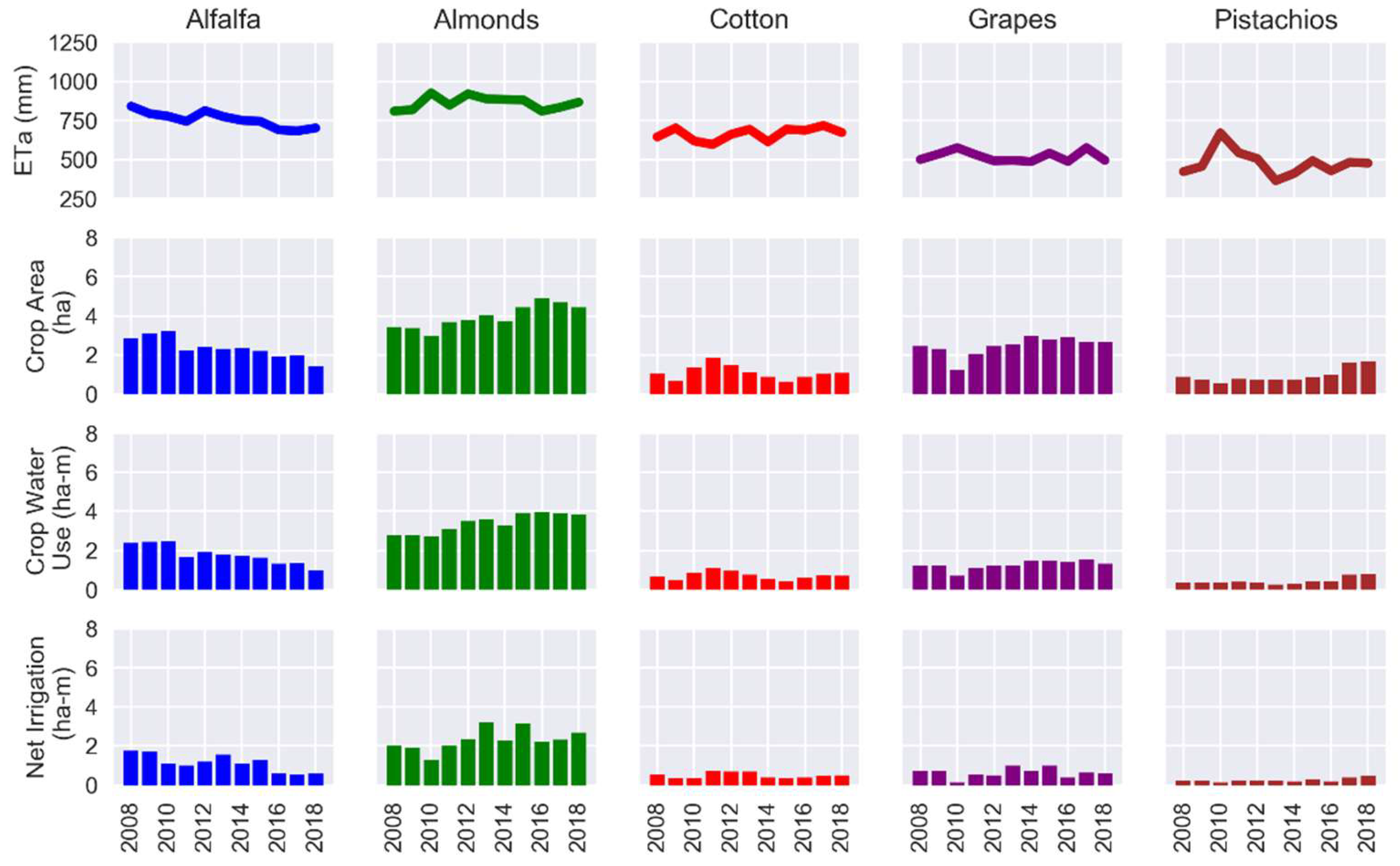
Figure 4.
Kern County showing (a) 1999 annual total SSEBop ETa, (b) major commodity parcels in 1999 identified by Kern County Department of Agriculture and Measurement Standards and filtered by maximum NDVI ≥ 0.5, (c) 2018 annual total SSEBop ETa, and (d) major commodity parcels in 2018 identified by Kern County Department of Agriculture and Measurement Standards and filtered by maximum NDVI ≥ 0.5.
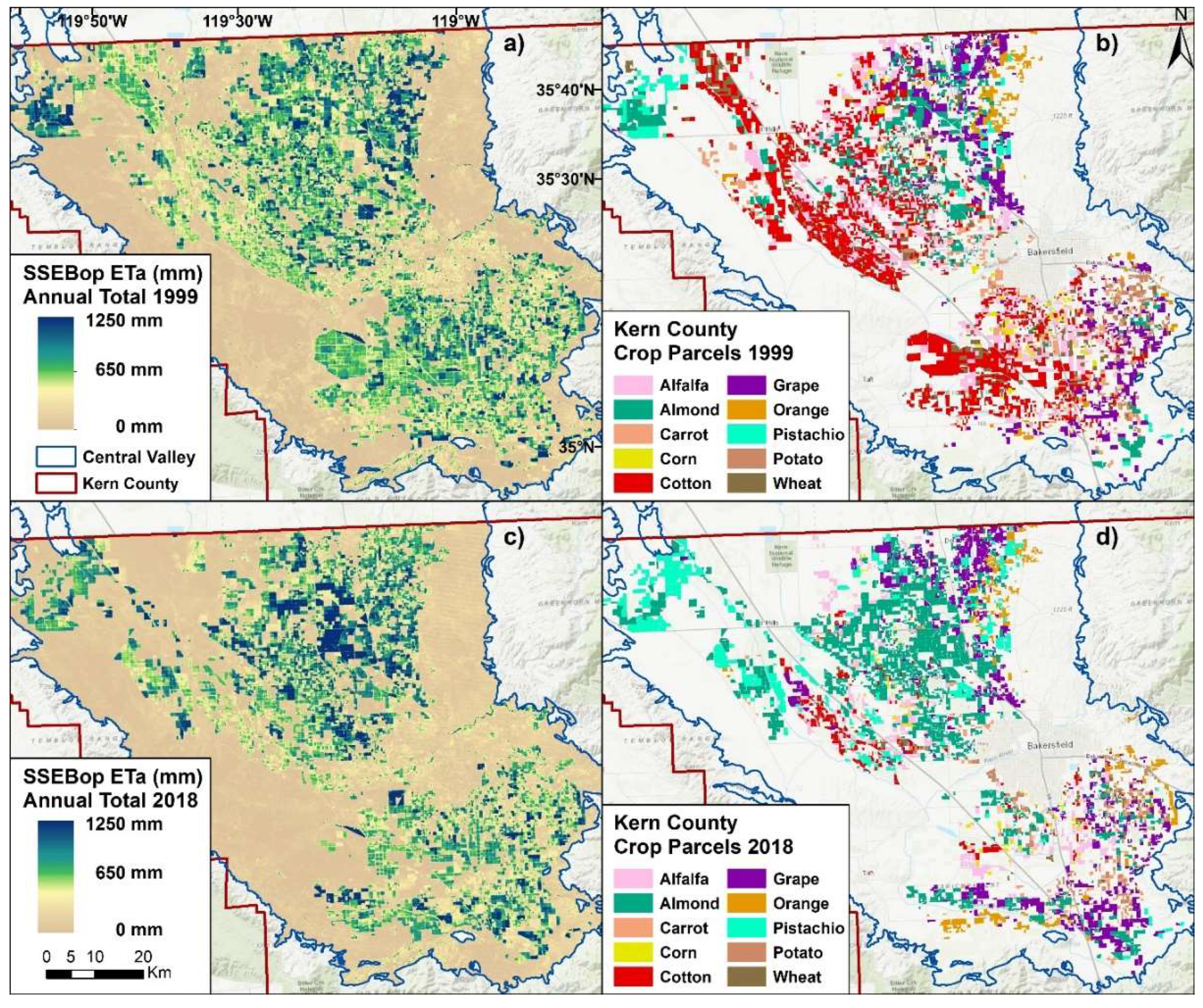
Figure 5.
The top five crops in Kern County from 1999 to 2018 showing the SSEBop ETa mean (in mm) for the USDA-NASS CDL crop type, the bias-corrected area estimate (in hectares), water use volume (ha-m) and the net irrigation (ha-m) in hectare-meters. The area, water use, and net irrigation are scaled by 10,000 (i.e., 4 ha-m corresponds to 40,000 ha-m). 1 hectare = 2.47 acres. 1 hectare-meter = 8.107 acre-feet.
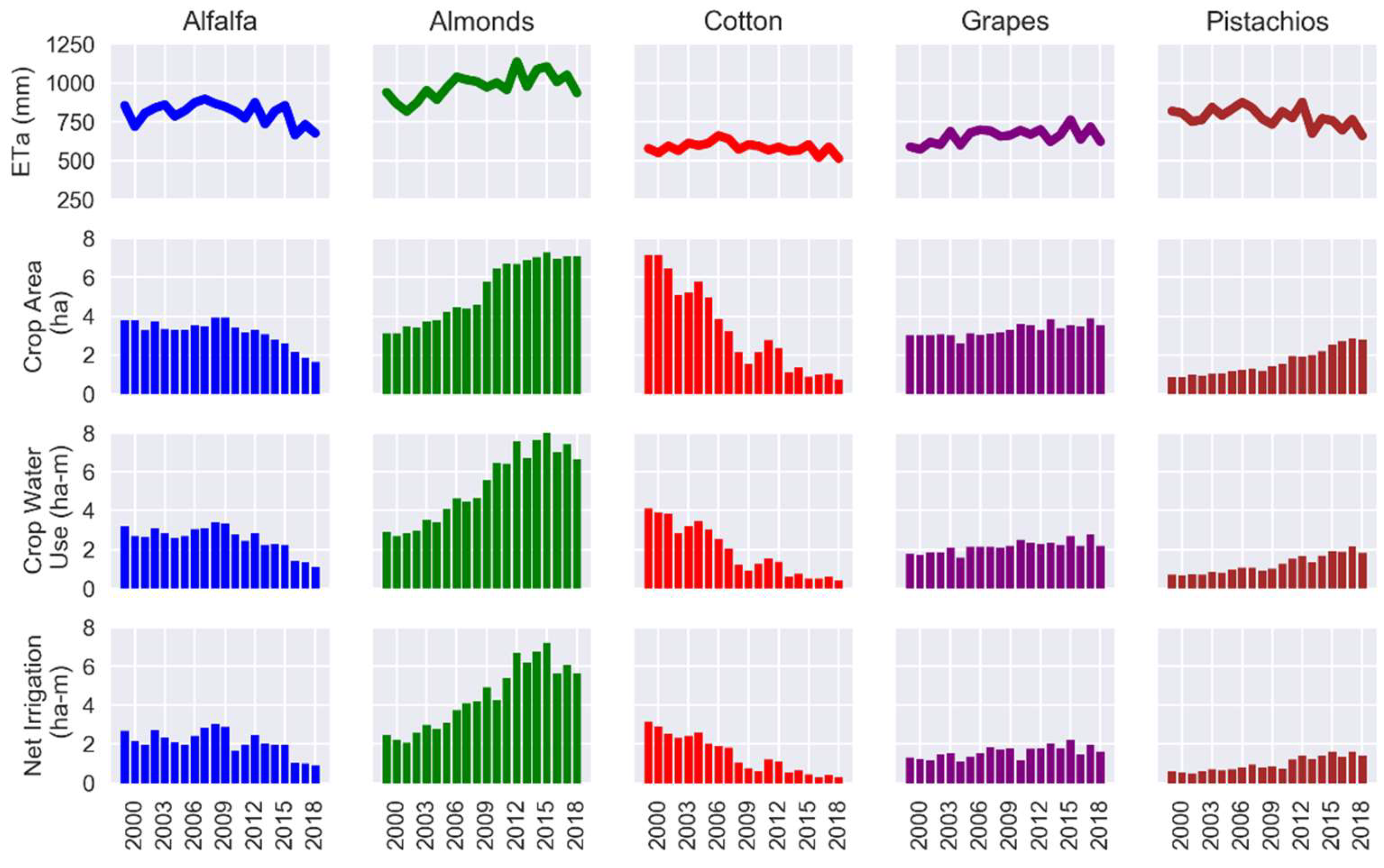
Figure 6.
Pixel-based Mann–Kendall trend analysis for all of Kern County based on annual SSEBop ETa from 1999 to 2018. The above graphic shows (a) the 20-year (1999–2018) mean annual total SSEBop ETa, (b) the Theil–Sen slope statistic on a per-pixel basis for the statistically significant pixels where the MK test p-value < 0.05 (95% confidence).

Figure 7.
Eight crop parcels that are identified as cotton fields in 1999–2003 but fields 1–4 transition to uncultivated agriculture and parcels 5–8 transition to almonds. Graphic shows (a) the current Google Earth imagery for the selected parcels, (b) the statistically significant pixels of the 1999–2018 Theil–Sen slope (blue indicates increasing slope and red indicated decreasing slope), and c the total water use for each of eight fields from 1999 to 2018.


Table 1.
Comparison of the area counts between the USDA-NASS Generalized Cropland Data Layer (CDL) and the aggregated county crop acreage reports from 2008 to 2017 for the top 10 crops in the Central Valley showing: (1) the average crop area in hectares from pixel-counting the generalized CDL, (2) the average crop area from the aggregated crop reports, and (3) the bias percentage that was used to bias-correct the CDL area to calculate water use between 2008 and 2018.
| Crop Type | CDL 1 | Crop Reports 1 | % Bias |
|---|---|---|---|
| Alfalfa | 285,164 | 247,669 | 15% |
| Almonds | 415,498 | 392,967 | 6% |
| Corn | 83,820 | 62,504 | 34% |
| Cotton | 111,169 | 108,328 | 3% |
| Grapes | 216,628 | 244,110 | −11% |
| Oranges | 57,601 | 65,721 | −12% |
| Pistachios | 75,978 | 90,929 | −16% |
| Rice | 215,794 | 208,871 | 3% |
| Walnuts | 121,829 | 126,944 | −4% |
| Winter Wheat | 155,343 | 129,594 | 20% |
1 In hectares (ha). 1 hectare = 2.47 acres.
Table 2.
Summary statistics of the final bias-corrected area estimates for the top 10 major crops in the Central Valley from 2008 to 2018 ordered by mean area including: (1) the 2008–2018 mean crop area in hectares, (2) the crop area in 2008 including the percentage of the total, (3) the crop area in 2018 including the percentage of the total, (4) the % change in crop area between 2008 and 2018, and (5) the mean crop area during the 2012–2016 California drought including the percent deviation from the mean.
| Crop Type | Mean Crop Area (ha) 1 | 2008 Crop Area (ha) 1 [%] | 2018 Crop Area (ha) 1 [%] | % Change | 2012–2016 Drought (ha) 1 [%] |
|---|---|---|---|---|---|
| Almonds | 395,204 | 343,695 [21%] | 445,249 [27%] | 30% | 417,652 [6%] |
| Grapes | 246,339 | 243,992 [15%] | 268,246 [16%] | 10% | 273,978 [11%] |
| Alfalfa | 235,705 | 283,905 [18%] | 141,768 [9%] | −50% | 223,405 [−5%] |
| Rice | 208,336 | 210,712 [13%] | 200,805 [12%] | −5% | 203,405 [−2%] |
| Walnuts | 130,527 | 92,920 [6%] | 161,005 [10%] | 73% | 129,912 [< −1%] |
| Winter Wheat | 118,101 | 146,169 [9%] | 62,256 [4%] | −57% | 108,738 [−8%] |
| Cotton | 109,195 | 104,663 [6%] | 107,219 [7%] | 2% | 99,718 [−9%] |
| Pistachios | 93,545 | 87,790 [5%] | 167,678 [10%] | 91% | 81,230 [−13%] |
| Corn | 62,738 | 69,604 [4%] | 59,031 [4%] | −15% | 59,411 [−5%] |
| Oranges | 27,152 | 26,837 [2%] | 18,619 [1%] | −31% | 26,810 [−1%] |
1 In hectares (ha). 1 hectare = 2.47 acres.
Table 3.
Simple Mann–Kendall trend test results for CDL crop area in the Central Valley from 2008 to 2018 for the top 10 major crops showing: (1) Mann–Kendall trend statistic, (2) p-value, (3) Theil–Sen slope (ha/year) from 2008 to 2018, and (4) the significant trend where (+) and (−) indicate statistically significant increasing or decreasing trends, respectively, where the p-value is less than 0.05 and (#) signifies the trend is not statistically significant and the p-value is greater than 0.05.
| Crop Type | MK Statistic | p-Value | Theil–Sen Slope (ha/yr) 1 | Trend 2 |
|---|---|---|---|---|
| Alfalfa | −39 | 0.003 | −12,429 | − |
| Almonds | 39 | 0.003 | 16,327 | + |
| Corn | −21 | 0.119 | −3543 | # |
| Cotton | −9 | 0.533 | −2038 | # |
| Grapes | 29 | 0.029 | 6119 | + |
| Oranges | −1 | 1.000 | −48 | # |
| Pistachios | 27 | 0.043 | 6635 | + |
| Rice | −23 | 0.087 | −3411 | # |
| Walnuts | 49 | 0.000 | 6668 | + |
| Winter Wheat | −37 | 0.005 | −7770 | − |
1 In hectares (ha). 1 hectare = 2.47 acres, 2 Durbin–Watson statistic shows no serial correlation for the statistically significant trends.
Table 4.
Volumetric water use estimates for the top 10 major crops in the Central Valley from 2008 to 2018 ordered by the mean including: (1) the 2008–2018 mean water use, (2) the water use in 2008 including the percentage of the total, (3) the water use in 2018 including the percentage of the total, (4) the % change in crop water use between 2008 and 2018, and (5) the mean crop water use during the 2012–2016 California drought and percent deviation from the mean.
| Crop Type | Mean Water Use (ha-m) 1 | 2008 Water Use (ha-m) 1 [%] | 2018 Water Use (ha-m) 1 [%] | % Change | 2012–2016 Drought (ha-m) 1 [%] |
|---|---|---|---|---|---|
| Almonds | 339,506 | 277,707 [23%] | 385,230 [33%] | 39% | 364,074 [7%] |
| Rice | 218,544 | 247,717 [21%] | 197,711 [17%] | −20% | 213,144 [−2%] |
| Alfalfa | 179,606 | 238,316 [20%] | 99,308 [9%] | −58% | 168,856 [−6%] |
| Grapes | 126,840 | 121,819 [10%] | 132,561 [11%] | 9% | 136,772 [8%] |
| Walnuts | 111,442 | 89,498 [7%] | 130,072 [11%] | 45% | 110,900 [< −1%] |
| Cotton | 71,508 | 67,374 [6%] | 71,994 [6%] | 7% | 66,533 [−7%] |
| Winter Wheat | 47,386 | 64,842 [5%] | 18,601 [2%] | −71% | 40,980 [−14%] |
| Pistachios | 44,123 | 37,028 [3%] | 79,774 [7%] | 115% | 35,733 [−19%] |
| Corn | 40,023 | 46,284 [4%] | 34,039 [3%] | −26% | 38,042 [−5%] |
| Oranges | 17,913 | 17,714 [1%] | 10,940 [1%] | −38% | 16,825 [−6%] |
1 In hectare-meters (ha-m). 1 hectare-meter = 8.107 acre-feet.
Table 5.
Simple Mann–Kendall trend test results for CDL crop water use by volume in the Central Valley from 2008 to 2018 for the top 10 major crops showing: (1) Mann–Kendall trend statistic, (2) p-value, (3) Theil–Sen slope (ha-m/yr) from 2008 to 2018, and (4) the significant trend where (+) and (−) indicate statistically significant increasing or decreasing trends, respectively, where the p-value is less than 0.05 and (#) signifies the trend is not statistically significant and the p-value is greater than 0.05.
| Crop Type | MK Statistic | p-Value | Theil–Sen Slope (ha-m/yr) 1 | Trend 2 |
|---|---|---|---|---|
| Alfalfa | −41 | 0.002 | −13,901 | − |
| Almonds | 35 | 0.008 | 13,488 | + |
| Corn | −23 | 0.087 | −2756 | # |
| Cotton | −7 | 0.640 | −841 | # |
| Grapes | 31 | 0.020 | 4042 | + |
| Oranges | −13 | 0.350 | −382 | # |
| Pistachios | 25 | 0.062 | 1963 | # |
| Rice | −27 | 0.043 | −5433 | − |
| Walnuts | 43 | 0.001 | 4300 | + |
| Winter Wheat | −35 | 0.008 | −4086 | − |
1 In hectare-meters (ha-m). 1 hectare-meter = 8.107 acre-feet, 2 Durbin–Watson statistic shows no serial correlation for the statistically significant trends.
Table 6.
Summary statistics of the crop area estimates for the top 10 major crops in Kern County from 1999 to 2018 ordered by the mean including: (1) the mean of the 1999–2018 period, (2) the crop area in 1999 and the percentage of the total crop area, (3) the crop area in 2018 and the percentage of the total crop area, (4) the change in crop area between 1999 and 2018, and (5) the mean crop area during the 2012–2016 California drought and percent deviation from the mean.
| Crop Type | Mean Crop Area (ha) 1 | 1999 Crop Area (ha) 1 [%] | 2018 Crop Area (ha) 1 [%] | % Change | 2012–2016 Drought (ha) 1 [%] |
|---|---|---|---|---|---|
| Almonds | 53,126 | 31,213 [14%] | 70,924 [38%] | 127% | 69,662 [31%] |
| Cotton | 32,957 | 71,264 [32%] | 7,603 [4%] | −89% | 13,343 [−60%] |
| Grapes | 32,778 | 30,261 [13%] | 35,141 [19%] | 16% | 34,951 [7%] |
| Alfalfa | 31,652 | 37,568 [17%] | 16,438 [9%] | −56% | 27,922 [−12%] |
| Pistachios | 16,247 | 8536 [4%] | 27,908 [15%] | 227% | 22,693 [40%] |
| Oranges | 11,305 | 7861 [3%] | 11,484 [6%] | 46% | 12,565 [11%] |
| Wheat | 9247 | 16,391 [7%] | 2885 [2%] | −82% | 5566 [−40%] |
| Carrots | 8952 | 10,964 [5%] | 5537 [3%] | −49% | 8203 [−8%] |
| Corn | 5597 | 4633 [2%] | 2622 [1%] | −43% | 5398 [−4%] |
| Potatoes | 4913 | 7306 [3%] | 6293 [3%] | −14% | 4216 [−14%] |
1 In hectares (ha). 1 hectare = 2.47 acres.
Table 7.
Simple Mann–Kendall trend results for the area of 10 major commodities in Kern County from 1999 to 2018 showing: (1) Mann–Kendall trend statistic, (2) p-value, (3) Theil–Sen slope (in hectares) from 1999 to 2018, and (4) the significant trend where (+) and (−) indicate statistically significant increasing or decreasing, respectively, trends where the p-value is less than 0.05 and (#) signifies the trend is not statistically significant and the p-value is greater than 0.05.
| Crop Type | MK Statistic | p-Value | Theil–Sen Slope (ha/yr) 1 | Trend 2 |
|---|---|---|---|---|
| Alfalfa | −113 | 0.000 | −758 | − |
| Almonds | 175 | 0.000 | 2465 | + |
| Carrots | −101 | 0.001 | −180 | − |
| Corn | −62 | 0.048 | −116 | − |
| Cotton | −159 | 0.000 | −3589 | − |
| Grapes | 123 | 0.000 | 358 | + |
| Oranges | 109 | 0.000 | 227 | + |
| Pistachios | 179 | 0.000 | 1095 | + |
| Potatoes | −71 | 0.023 | −165 | − |
| Wheat | −111 | 0.000 | −560 | − |
1 In hectares (ha). 1 hectare = 2.47 acres, 2 Durbin–Watson statistic shows no serial correlation for the statistically significant trends.
Table 8.
Summary statistics of the crop water use estimates for the top 10 major crops in Kern County Figure 1999. to 2018 ordered by mean including: (1) the mean of the 1999–2018 period, (2) the crop area in 1999 and the percentage of the total crop area, (3) the crop area in 2018 and the percentage of the total crop area, (4) the change in crop area between 1999 and 2018, and (5) the mean crop area during the 2012–2016 California drought and percent deviation from the mean.
| Crop Type | Mean Water Use (ha-m) 1 | 1999 Water Use (ha-m) 1 [%] | 2018 Water Use (ha-m)1 [%] | % Change | 2012–2016 Drought (ha-m) 1 [%] |
|---|---|---|---|---|---|
| Almonds | 52,782 | 29,275 [18%] | 66,243 [48%] | 126% | 73,827 [40%] |
| Alfalfa | 25,735 | 32,015 [20%] | 11,095 [8%] | −65% | 22,203 [−14%] |
| Grapes | 21,574 | 17,790 [11%] | 21,823 [16%] | 23% | 23,605 [9%] |
| Cotton | 19,383 | 41,075 [26%] | 3,895 [3%] | −91% | 7,600 [−61%] |
| Pistachios | 12,451 | 6975 [4%] | 18,405 [13%] | 164% | 17,007 [37%] |
| Oranges | 9740 | 7820 [5%] | 8198 [6%] | 5% | 10,199 [5%] |
| Wheat | 5691 | 10,278 [6%] | 1411 [1%] | −86% | 3524 [−38%] |
| Carrots | 4989 | 6086 [4%] | 2652 [2%] | −56% | 4430 [−11%] |
| Corn | 3524 | 3047 [2%] | 1349 [1%] | −56% | 3451 [−2%] |
| Potatoes | 2444 | 3973 [3%] | 3134 [2%] | −21% | 2009 [−18%] |
1 In hectare-meters (ha-m). 1 hectare-meter = 8.107 acre-feet.
Table 9.
Simple Mann–Kendall trend results for crop water use by volume of 10 major commodities in Kern County from 1999 to 2018 showing: (1) Mann–Kendall trend statistic, (2) p-value, (3) Theil–Sen slope (in hectare-meters) from 1999 to 2018, and (4) the significant trend where (+) and (−) indicate statistically significant increasing or decreasing, respectively, trends where the p-value is less than 0.05 and (#) signifies the trend is not statistically significant and the p-value is greater than 0.05.
| Crop Type | MK Statistic | p-Value | Theil–Sen Slope (ha-m/yr) 1 | Trend 2 |
|---|---|---|---|---|
| Alfalfa | −94 | 0.003 | −698 | − |
| Almonds | 154 | 0.000 | 3035 | + |
| Carrots | −58 | 0.064 | −81 | # |
| Corn | −48 | 0.127 | −65 | # |
| Cotton | −160 | 0.000 | −2107 | − |
| Grapes | 124 | 0.000 | 410 | + |
| Oranges | 68 | 0.030 | 115 | + |
| Pistachios | 162 | 0.000 | 744 | + |
| Potatoes | −88 | 0.005 | −82 | − |
| Wheat | −100 | 0.001 | −352 | − |
1 In hectare-meters (ha-m). 1 hectare-meter = 8.107 acre-feet, 2 Durbin–Watson statistic shows no serial correlation for the statistically significant trends.
© 2019 by the authors. Licensee MDPI, Basel, Switzerland. This article is an open access article distributed under the terms and conditions of the Creative Commons Attribution (CC BY) license (http://creativecommons.org/licenses/by/4.0/).
Share and Cite
MDPI and ACS Style
Schauer, M.; Senay, G.B. Characterizing Crop Water Use Dynamics in the Central Valley of California Using Landsat-Derived Evapotranspiration. Remote Sens. 2019, 11, 1782. https://0-doi-org.brum.beds.ac.uk/10.3390/rs11151782
AMA Style
Schauer M, Senay GB. Characterizing Crop Water Use Dynamics in the Central Valley of California Using Landsat-Derived Evapotranspiration. Remote Sensing. 2019; 11(15):1782. https://0-doi-org.brum.beds.ac.uk/10.3390/rs11151782
Chicago/Turabian StyleSchauer, Matthew, and Gabriel B. Senay. 2019. "Characterizing Crop Water Use Dynamics in the Central Valley of California Using Landsat-Derived Evapotranspiration" Remote Sensing 11, no. 15: 1782. https://0-doi-org.brum.beds.ac.uk/10.3390/rs11151782
Note that from the first issue of 2016, this journal uses article numbers instead of page numbers. See further details here.