Article

Dissecting Performances of PERSIANN-CDR Precipitation Product over Huai River Basin, China

1
Collaborative Innovation Center on Forecast and Evaluation of Meteorological Disasters/Key Laboratory of Meteorological Disaster, Ministry of Education/International Joint Research Laboratory on Climate and Environment Change, Nanjing University of Information Science and Technology, Nanjing 210044, China
2
Ningbo Meteorological Bureau, Ningbo 315012, China
3
School of Applied Meteorology, Nanjing University of Information Science and Technology, Nanjing 210044, China
4
Climate Center of Jiangsu Province, Meteorological Bureau, Nanjing 210008, China
5
School of Geographical Sciences, Nanjing University of Information Science and Technology, Nanjing 210044, China
*
Author to whom correspondence should be addressed.
Remote Sens. 2019, 11(15), 1805; https://0-doi-org.brum.beds.ac.uk/10.3390/rs11151805
Submission received: 10 June 2019 / Revised: 29 July 2019 / Accepted: 30 July 2019 / Published: 1 August 2019
(This article belongs to the Special Issue Precipitation and Water Cycle Measurements Using Remote Sensing)

Abstract

:
Satellite-based precipitation products, especially those with high temporal and spatial resolution, constitute a potential alternative to sparse rain gauge networks for multidisciplinary research and applications. In this study, the validation of the 30-year Precipitation Estimation from Remotely Sensed Information using Artificial Neural Networks-Climate Data Record (PERSIANN-CDR) daily precipitation dataset was conducted over the Huai River Basin (HRB) of China. Based on daily precipitation data from 182 rain gauges, several continuous and categorical validation statistics combined with bias and error decomposition techniques were employed to quantitatively dissect the PERSIANN-CDR performance on daily, monthly, and annual scales. With and without consideration of non-rainfall data, this product reproduces adequate climatologic precipitation characteristics in the HRB, such as intra-annual cycles and spatial distributions. Bias analyses show that PERSIANN-CDR overestimates daily, monthly, and annual precipitation with a regional mean percent total bias of 11%. This is related closely to the larger positive false bias on the daily scale, while the negative non-false bias comes from a large underestimation of high percentile data despite overestimating lower percentile data. The systematic sub-component (error from high precipitation), which is independent of timescale, mainly leads to the PERSIANN-CDR total Mean-Square-Error (TMSE). Moreover, the daily TMSE is attributed to non-false error. The correlation coefficient (R) and Kling–Gupta Efficiency (KGE) respectively suggest that this product can well capture the temporal variability of precipitation and has a moderate-to-high overall performance skill in reproducing precipitation. The corresponding capabilities increase from the daily to annual scale, but decrease with the specified precipitation thresholds. Overall, the PERSIANN-CDR product has good (poor) performance in detecting daily low (high) rainfall events on the basis of Probability of Detection, and it has a False Alarm Ratio of above 50% for each precipitation threshold. The Equitable Threat Score and Heidke Skill Score both suggest that PERSIANN-CDR has a certain ability to detect precipitation between the second and eighth percentiles. According to the Hanssen–Kuipers Discriminant, this product can generally discriminate rainfall events between two thresholds. The Frequency Bias Index indicates an overestimation (underestimation) of precipitation totals in thresholds below (above) the seventh percentile. Also, continuous and categorical statistics for each month show evident intra-annual fluctuations. In brief, the comprehensive dissection of PERSIANN-CDR performance reported herein facilitates a valuable reference for decision-makers seeking to mitigate the adverse impacts of water deficit in the HRB and algorithm improvements in this product.

1. Introduction

Precipitation, as an important hydrometeorological variable, plays a foremost role in the energy and water cycle, and thus in weather, climatology, hydrology, ecosystems, and even the Earth system [1,2]. It is deemed essential for life on the Earth, especially for humans, mainly because the overwhelming majority of freshwater resources over land originate from precipitation. As such, precipitation measurements are of great interest to various scientific fields, such as atmospheric, ecological, hydrological, agricultural, environmental, and economic studies, although their purposes and intentions are tremendously different [2,3,4,5,6,7,8]. For example, continuous and long-term precipitation observations are fundamental not only to climate change research, but also to the establishment of reasonable policies and actions that address climate change-related adverse impacts (e.g., intensifying droughts and floods) [9,10,11,12,13,14]. Despite this paramount importance, there still exist immense challenges for obtaining accurate, uninterrupted, and uniform precipitation measurements on regional and global scales, consequently hindering developments in sciences and human societies [6,15,16,17,18,19].
In general, there are three pathways to obtain precipitation data [19]: Direct observation using various gauges (e.g., tipping-bucket rain gauges), and retrievals from radar and satellite techniques (i.e., using relationships between precipitation and infrared (IR), visible (VIS), and/or microwave (MW) radiance signals). Undoubtedly, these gauge precipitation datasets serve as essential sources of information for various scientific disciplines, particularly for studies of climate change (e.g., Reference [20]). It is noted that directly gauging precipitation is available in specific places, with some records dating back to several thousand years [21], but most areas have no ground sites as a result of inaccessibility and higher costs for installations and maintenance. This limits the representativeness of gauge precipitation, because precipitating weather systems generally have high spatial and temporal variability [2,7,22,23,24,25,26]. In fact, many important applications have different and specific requirements for the accuracy, connectivity, timeliness, and temporal and spatial resolutions of precipitation datasets. Thus, for better understanding of hydrometeorological processes, detailed precipitation information on a broad range of temporal and spatial scales is necessary [2,25]. For example, local, fine-scale data with low data latency are adequate for flash flood studies, and long-term measurements are imperative for drought research. For drawing precise conclusions in climate studies, measurement accuracy and homogeneity are more important than other requirements, while daily records suffice for agricultural applications. In the past decades, gaps in direct precipitation observations have been filled to a great extent by technologically sophisticated radars and MW sensors. The ability to provide precipitation products with more extensive coverage (even across the globe) and higher temporal resolution has been especially improved [4]. Because of the backwardness of radar technology in some countries, radar blockage, due to topography, and the nearly negligible radar measurements overseas, satellite-based precipitation estimates have become the most attractive and viable approach to fulfill various requirements of academic studies and practical applications [19,27,28,29].
Unlike rain gauges, satellites cannot directly measure precipitation; instead, estimates are calculated from radiance information received by satellite-carried sensors (i.e., VIS/IR sensors on geostationary (GEO) and low Earth orbit (LEO) satellites, and passive (PMW) and active MW sensors on LEO satellites) using various statistical and/or physics-based retrieval algorithms [30,31,32]. For precipitation estimates only using VIS/IR signals, such products inherit the advantages of wide coverage, and fine temporal and spatial scales, which are important for monitoring precipitation extremes and the related disastrous hydrometeorological events (e.g., floods). However, great uncertainties still exist in these products, mainly because of the indirect link between cloud-top brightness temperature (Tb) and surface precipitation [28,33]. Different from VIS/IR-based techniques, the more robust relationship between observations and MW signals, which can better represent hydrometeor content within the atmosphere column, is employed by MW-based algorithms, and thus rainfall estimates are more accurate. Notably, MW sensors are on LEO satellites, and, therefore, they have a coarse temporal resolution, thereby leading to large sampling errors for short-term rainfall events [34,35]. In order to compressively take advantage of the strengths of these two algorithms for more accurate precipitation estimates, the most current techniques combine VIS/IR and MW signals [36]. As a result, great efforts have been devoted to generating global or quasi-global satellite-based precipitation datasets with different temporal (e.g., hourly, 3-hourly, daily, and monthly) and spatial (e.g., 0.1°, 0.25°, and 0.5°) resolutions. Examples include Tropical Rainfall Measuring Mission (TRMM) Multi-Satellite Precipitation Analysis (TMPA; no longer operational) products (e.g., near-real-time (3B42RT) and gauge-adjusted versions (3B42v7)) from the National Aeronautics and Space Administration (NASA) Goddard Space Flight Center (GSFC; [37]); the National Oceanic and Atmospheric Administration (NOAA) Climate Prediction Center (CPC) morphing technique (CMORPH; [28]), which has both satellite-only and gauge-adjusted products [38]; the satellite-only Global Satellite Mapping of Precipitation Microwave-IR Combined Product (GSMaP-MVK) and gauge-adjusted (GSMaP-Gauge) datasets produced at the Earth Observation Research Center (EORC) of the Japan Aerospace Exploration Agency (JAXA; [35]); the Precipitation Estimation from Remotely Sensed Information Using Artificial Neural Networks (PERSIANN; [6,39]), including both satellite-only (i.e., PERSIANN and PERSIANN-Cloud Classification System (CCS)) and gauge-adjusted versions (PERSIANN-Climate Data Record (CDR)); the Integrated Multi-satellite Retrievals for Global Precipitation Measurement (IMERG), which contributes higher-resolution near-real-time and gauge-adjusted global precipitation estimates [40]; and the Climate Hazards Group InfraRed Precipitation with Station Data (CHIRPS), which is a new land-only climatic database for precipitation [41]. Despite that, the existing satellite-based products still remain some intrinsic issues at least now, such as susceptible to systematic biases [36,42,43]. For overcoming or at least reducing the uncertainties within the satellite-based precipitation estimates, in more recent Beck et al. [44] developed a new global Multi-Source Weighted-Ensemble Precipitation (MSEWP) rainfall dataset through merging the highest-quality precipitation products sources available (including various satellite-based, reanalysis and gauge-based datasets) as a function of timescale and location. Undoubtedly, these products provide abundant data sources for hydrometeorological studies and applications at regional and global scales.
Before operational use, the selected satellite-based precipitation products need to be systematically validated and then properly corrected using dependable reference datasets. According to specific needs and goals, the quantitative evaluation of satellite-based precipitation estimates has become a prime subject of studies, and these products have been extensively assessed across the globe on different temporal and spatial scales with a variety of statistical metrics [45,46,47,48,49,50,51,52,53,54]. For example, Zeng et al. [52] evaluated five satellite-based precipitation products with gauge measurements from 2005 to 2013 over China, and suggested that GSMaP generally outperformed the other products, despite underestimation. Using two gauge-scarce basins as the study regions on the Tibetan Plateau of China, Bai and Liu [53] analyzed five satellite-based precipitation products’ capacities in simulating streamflow by comparing simulations with gauge measurements. They found that these products showed an accurate and comparable performance despite significantly different estimates of the precipitation amount. Results from Mayor et al. [48] indicated that the IMGER precipitation product on daily and seasonal scales generally performed better than that on the hourly scale over Mexico. In brief, many interesting findings have been produced although these studies focus on different precipitation products, precipitation characteristics (e.g., light and heavy rainfall events), temporal scales (e.g., daily, monthly, and seasonal), statistical metrics (e.g., bias and correlation coefficient), and regions/basins [31,38,55]. In sum, these conclusions have provided valuable information for the theoretical understanding and development of satellite-retrieved methodologies and their practical applications.
With exacerbating climate change, especially successive and rapid warming, a growing body of evidence suggests that the hydrometeorological extremes (e.g., droughts, floods, and rainfall extremes) over the mainland of China have changed, but they have been mainly characterized by significant regional differences [14]. In China, the Huai River Basin (HRB) is a very important food production region—where the arable area and crop yields are about 11.7% and 17.4% of the nation’s total, respectively [56]. However, this basin frequently suffers from droughts, with drought-affected arable areas exceeding 20,000 km2 in 14 years during the period of 1949–2000 and local and regional droughts occurring nearly every year. Statistics have indicated that the accumulative arable area affected by drought disasters in the HRB has increased by 53% between 1991 and 2000 relative to the period of 1981–1990, implying that droughts have intensified and occurred more frequently [57]. In addition, the HRB is a typical water-deficient region in China: Its water resources per capita are lower than a quarter of the national average [58]. Therefore, reasonably planning water resource management and agricultural irrigation schedules are very important for regional and even national food security and food production capacity. In short, reliable, long-term (records generally longer than 30 years), continuous, and relatively high spatiotemporal resolution precipitation information is of critical significance for practical applications in the HRB; and then the PERSIANN-CDR precipitation product is selected here for evaluation based on a high density (182) of observation sites. Many studies have assessed PERSIANN-CDR across the world, including some regions of China [59,60,61,62,63,64,65]. However, satellite-based precipitation products usually vary in biases, errors, and detection capabilities among regions, timescales, and rainfall intensities [38]. As a result, several questions should be answered before the use of PERSIANN-CDR in the HRB: (1) How does this product perform according to various continuous and categorical metrics? (2) Does PERSIANN-CDR performance differ among temporal scales (i.e., daily, monthly, and annual) and precipitation thresholds (i.e., from the first to ninth percentiles)? (3) To what extent do bias and error sub-components, which are obtained by related decomposition techniques, play a role in continuous metrics? The analyses of this study will serve as a valuable reference for decision-makers to mitigate the adverse impacts of water deficit in the HRB and even for algorithm developers of PERSIANN-CDR.

2. Data and Methodology
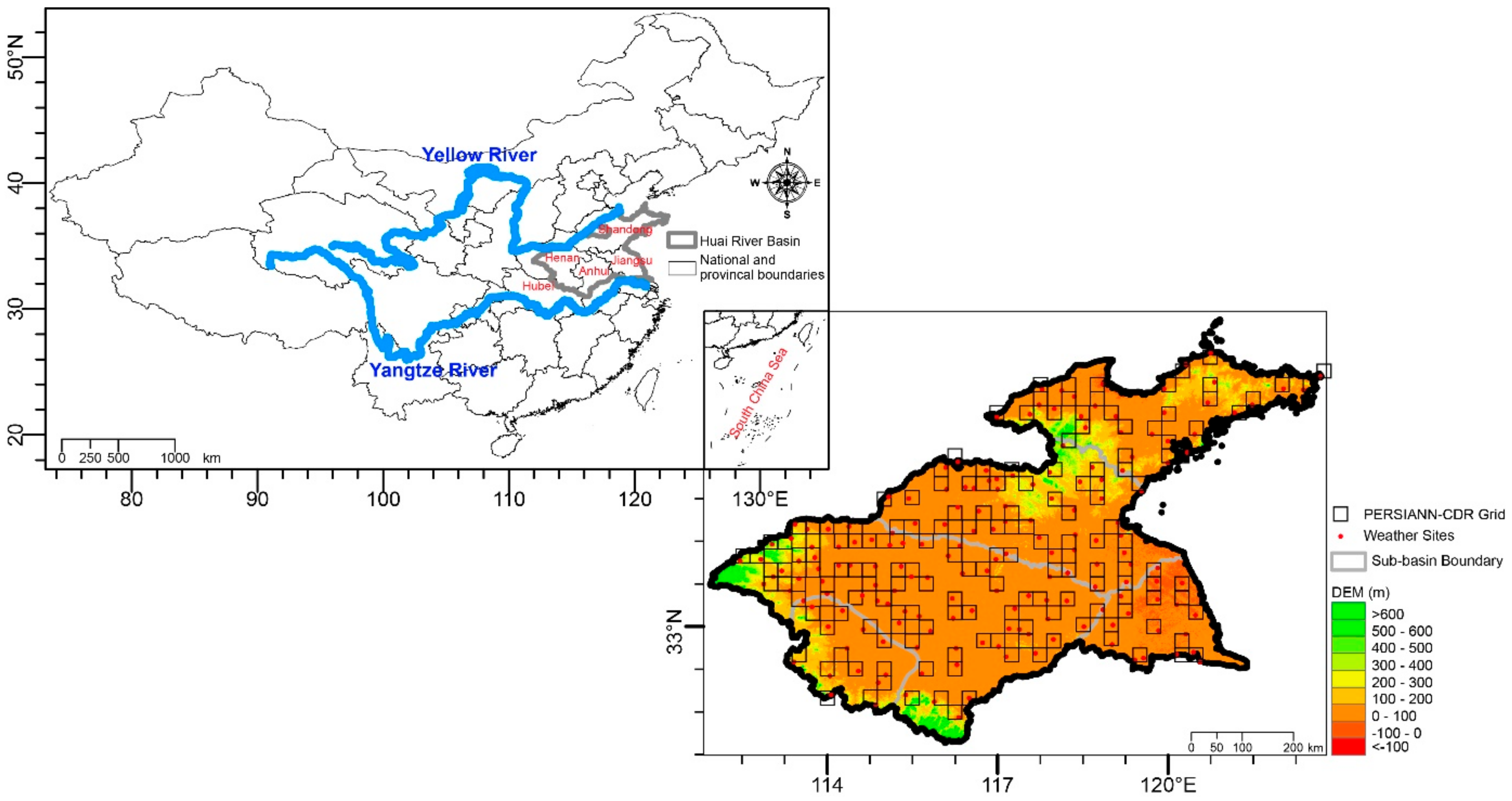
2.1. Study Region

The study region is the HRB (between 30–39°E and 111–123°E), located in eastern China between the Yellow River and the Yangtze River (Figure 1). Covering a drainage area of approximately 33,000 km2, the HRB mainly includes the northern parts of Jiangsu and Anhui, a small part of Hubei, and most of Shandong and Henan. As one of the ten water resource regions in China, the HRB has a vast plain with many lakes and depressions, and is moderately mountainous (general elevation ranging from 1000 to 2000 m above sea level) near the western boundary, mid-eastern part, and Shandong peninsula. A typical semi-humid monsoon climate with warm temperatures prevails in this basin, with regional average annual temperature and precipitation of about 14 °C and 806 mm, respectively. In the HRB, precipitation is concentrated in the Meiyu rain season of China (from mid-May to mid-October) and has large annual and seasonal variability [66]. Because of the unique climate and specific surface conditions, the HRB often suffers from flooding, waterlogging, drought, and storm surge disasters, especially in its middle and lower parts [66].

2.2. Data

Observed daily precipitation data from 1960 to 2012 at more than 200 gauge sites were collected from the China Meteorological Administration (CMA) to validate the PERSIANN-CDR precipitation product. Two data quality issues—missing values and inhomogeneity—were first resolved. Days with missing values were determined for each year and each site. Sites with data available for less than 330 days per year were removed, and missing values of the remaining sites were filled with data from nearby sites using the bilinear regression. Subsequently, the analyses of time series homogeneity were performed using the Pettitt test [67], and the sites with time series not passing the significance test (p< 0.05) were eliminated. After the data quality control, records from 182 sites remained (Figure 1). To match the gridded PERSIANN-CDR data, we followed Katiraie-Boroujerdy et al. [68] and processed the 182 sites into 176 grid boxes of 0.25° × 0.25° longitude by latitude. The final observational value for a certain grid box was computed by averaging the daily records of the gauge site(s) within the given grid. The sites and their corresponding grid boxes are shown in Figure 1.
The PERSIANN-CDR precipitation product is a new retrospective satellite-based dataset that was developed for the U.S National Climatic Data Center (NCDC) Climate Data Record program in NOAA [29]. This dataset provides near-global (60°S–60°N) daily precipitation estimates from 1983 to the present with a spatial resolution of 0.25° × 0.25°. The PERSIANN-CDR dataset is available for public use from the U.S NOAA National Centers for Environment Information (NCEI) at https://www.ncdc.noaa.gov/cdr/atmospheric/precipitation-persiann-cdr and the Centre for Hydrometeorology and Remote Sensing (CHRS) Data Portal at http://chrsdata.eng.uci.edu. For more details about the PERSIANN-CDR algorithm, readers can refer to Ashouri et al. [29]. In this study, the analysis time period is 1983–2012, when both the PERSIANN-CDR product and direct observations are available.

2.3. Methodology

To quantitatively evaluate the performance of PERSIANN-CDR estimates, we selected two extensively-used evaluation criteria—continuous and categorical measures (Table 1) [45,63,68,69,70,71]. Moreover, bias and error decomposition techniques were also used to explore the contributions of different sub-components of biases and errors to the total values, respectively [63,69,70,71,72].

Bias Decomposition

To determine the impacts of the PERSIANN-CDR product’s detection capability, we first decomposed the TB into three sub-components: The bias in successful detections (i.e., hits; HB or percent HB (pHB)), the bias, due to rainfall misses (MB or percent MB (pMB)), and the bias, due to false detections (FB or percent FB (pFB)), i.e.,
{ T B = H B + M B + F B , H B = 1 N i = 1 n H ( S i O i ) , M B = 1 N i = 1 n M ( S i O i ) , F B = 1 N i = 1 n F ( S i O i ) ,
where nH, nM, and nF are the number of samples corresponding to conditions of Si > 0 mm/day, and Oi > 0 mm/day, Si = 0 mm/day and Oi ≥ 0 mm/day, and Si ≥ 0 mm/day and Oi = 0 mm/day, respectively. HB can be further divided into two parts, HB0-1 and HB≥1; they reflect hit biases in successful detections of rainfall events with daily precipitation of 0–1 mm/day and ≥1 mm/day, respectively.
Additionally, the non-false bias (i.e., NFB = HB≥1 + MB) can also be separated into several components corresponding to different bins. This is useful for the in-depth understanding of biases from its distribution among various rain intensities. In this study, we selected daily and monthly OBS precipitation percentiles as the partition points of each bin, such as the bin between ith and (i+1)th percentiles (named [Pi, Pi+1)). This process is named percentile-based bias decomposition, and the sub-component for a certain bin can be expressed as
N F B = i = 0 9 B P i , i + 1 , B P i , i + 1 , = 1 N j = 0 n P i , i + 1 , ( S j O j ) ,
where BPi,i+1 represents bias within [Pi, Pi+1), whose number of samples is nPi,i+1. Notably, the daily percentiles are obtained using data in which OBS daily precipitation ≥ 1 mm/day (so, the daily P0 value is 1 mm/day). The percent values of HB, MB, FB, NFB, and BPi,i+1 (named pHB, pMB, pFB, pNFB, and pBPi,i+1) can be calculated by dividing by the OBS mean (i.e., O).Error Decomposition
According to previous studies (e.g., Reference [35]), the TMSE includes two components, i.e., systematic (MSEs) and random errors (MSEr), which are calculated by
T M S E = 1 N i = 1 N ( S i S ^ i ) 2 M S E r + 1 N i = 1 N ( S ^ i O i ) 2 M S E s .
Similar to bias decomposition, we can also get detection-based and percentile-based error sub-components.
Detection-based Error Sub-components:
{ T M S E = H M S E + M M S E + F M S E , H M S E = 1 N j = 1 n H ( S j O j ) 2 , M M S E = 1 N j = 1 n M ( S j O j ) 2 , F M S E = 1 N j = 1 n F ( S j O j ) 2 ,
where S ^ j is defined by the least-square linear regression, i.e., S ^ j = a + b · O j , with a and b denoting the intercept and slope, respectively. It is noteworthy that the regression equation for each grid box is established using all daily, monthly, or annual samples. Following HB decomposition, HMSE is also broken into HMSE0-1 and HMSE1 for respectively reflecting hit errors in successful detections of rainfall events with 0–1 mm/day and ≥1 mm/day. Then, non-false MSE (i.e., NFMSE) can be expressed as the sum of HMSE1 and MMSE.
Percentile-based Error Sub-components:
N F M S E = i = 0 9 M S E P i , i + 1 , M S E P i , i + 1 , = 1 N j = 1 n P i , i + 1 ( S j O j ) 2 ,
where HMSE, MMSE, and FMSE are errors in successful detections, errors, due to rainfall misses, and errors, due to false detection, respectively. MSEPi,i+1 represents the error for the bin of [Pi, Pi+1), as defined as above. The percent values of HMSE, MMSE, FMSE, NFMSE, and MSEPi,i+1 (named pHMSE, pMMSE, pFMSE, pNFMSE, and pMSEPi,i+1) can be obtained by dividing its value by TMSE. Notably, in this study, we calculated these selected validation metrics at 176 grid boxes, and utilize their means to detect PERSIANN-CDR performances in the HRB. Moreover, the box-plots for each validation metric in the following text are drawn using their estimates at all the grid boxes.

3. Results

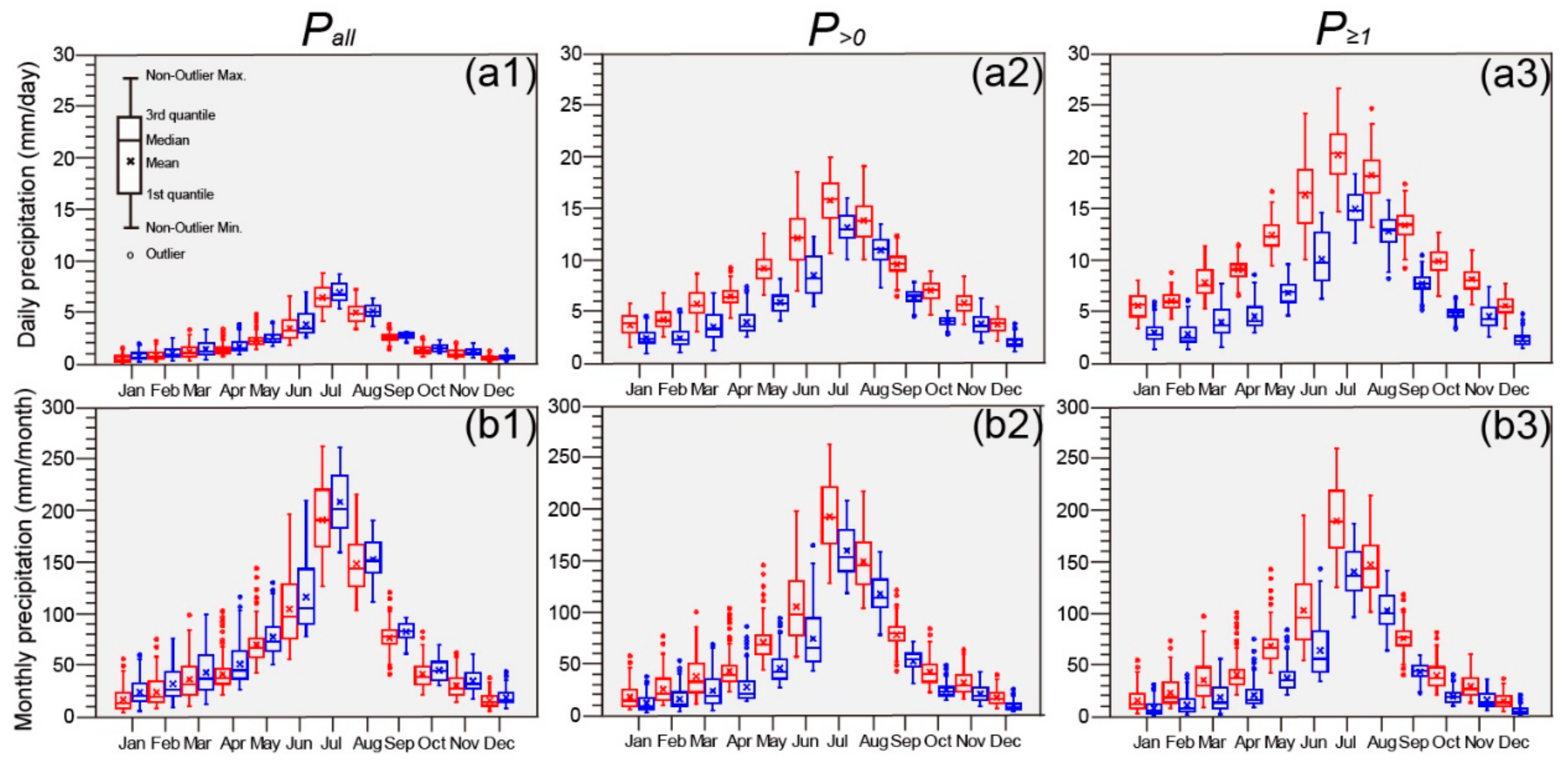
3.1. Climatologic Characteristics of Precipitation

As a first step, the 30-year mean daily, monthly, and annual Pall of OBS and PERSIANN-CDR were calculated by averaging over the HRB (Table 3), i.e., 2.21 vs. 2.45 mm/day, 67.24 vs. 74.66 mm/month, and 806.92 vs. 895.90 mm/year. To further investigate the intra-annual cycle of Pall, Figure 2(a1,a2) illustrates the results using the multi-year mean daily (monthly) data points. The OBS result reveals obvious seasonality, with higher values of Pall (> 3.50 mm/day or > 105.00 mm/month) from June to August, accompanied by greater spatial variability (larger spread between the first and third quantiles), and a peak in July (6.39 mm/day or 185.00 mm/month). The remaining months correspond to lower values (< 3.00 mm/day or < 71.00 mm/month) and relatively smaller spatial variability. Intuitively, PERSIANN-CDR can effectively reproduce the intra-annual changes in Pall, with a maximum (7.00 mm/day or 192.51 mm/month) in July and greater spatial variability. Figure 3(a1,b1,c1) show the spatial patterns of OBS multi-year mean Pall on daily, monthly, and annual scales, respectively. It is evident that despite different temporal scales, OBS Pall is generally characterized by a decrease from the southeast to northwest of the HRB. Comparison between OBS and PERSIANN-CDR (Figure 3(a1) vs. Figure 3(a2), Figure 3(b1) vs. Figure 3(b2), and Figure 3(c1) vs. Figure 3(c2)) suggests that PERSIANN-CDR can well capture the spatial distributions of climatological Pall on daily, monthly, and annual scales, with a spatial R larger than 0.94. Also, the spatial pattern of daily or monthly Pall for PERSIANN-CDR was compared with that of OBS for each month (not shown here). Except for August, when there is a reduction in OBS Pall from the coast to inland, Pall decreases from the southeast to northwest in the other moths. In each month, the spatial distribution of PERSIANN-CDR Pall matches well with that of OBS on daily or monthly scales, with a spatial R between 0.71 and 0.96. This indicates that this product performs well in capturing the intra-annual cycle of daily and monthly Pall in space.
We also compared multi-year means of OBS daily, monthly, and annual P>0 (P≥1) averaged over the HRB with those of PERSIANN-CDR (Table 3). Relative to HRB Pall, OBS multi-year mean daily P>0 (P≥1) increases because of the decreased number of days with OBS daily precipitation larger than 0 (1 mm/day) and unchanged (slightly changed) accumulative precipitation values, which can be reflected by OBS multi-year mean monthly and annual P>0 (P≥1; Table 3). Although PERSIANN-CDR multi-year mean daily P>0 (P≥1) also increases compared with Pall, its monthly and annual values decrease. This is mainly because that PERSIANN-CDR has lower daily estimates, and it missed rainfall events corresponding to OBS daily precipitation above 0 (1 mm/day). Similar to the intra-annual cycles of Pall on daily and monthly scales, P>0 values (Figure 2(a2,b2); P≥1, Figure 2(a3,b3)) are characterized by evident seasonality, i.e., an increase starting in January, a peak in July, and larger spatial variability in June–August. Moreover, OBS multi-year mean daily and monthly P>0 (P≥1) values are larger than the PERSIANN-CDR values for each month. In terms of the spatial distributions of multi-year mean daily, monthly, and annual P>0 (Figure 3(a3) vs. Figure 3(a4), Figure 3(b3) vs. Figure 3(b4), and Figure 3(c3) vs. Figure 3(c4); P≥1, Figure 3(a5) vs. Figure 3(a6), Figure 3(b5) vs. Figure 3(b6), and Figure 3(c5) vs. Figure 3(c6)), OBS and PERSIANN-CDR share similar features, i.e., P>0 (P≥1) decreasing from the southeast to northwest, with a spatial R above 0.65. Moreover, PERSIANN-CDR can also better reproduce the spatial patterns of daily and monthly P>0 (P≥1), with spatial R values ranging from 0.75 to 0.95 throughout the year (not shown).

3.2. Performance Based on Daily Data

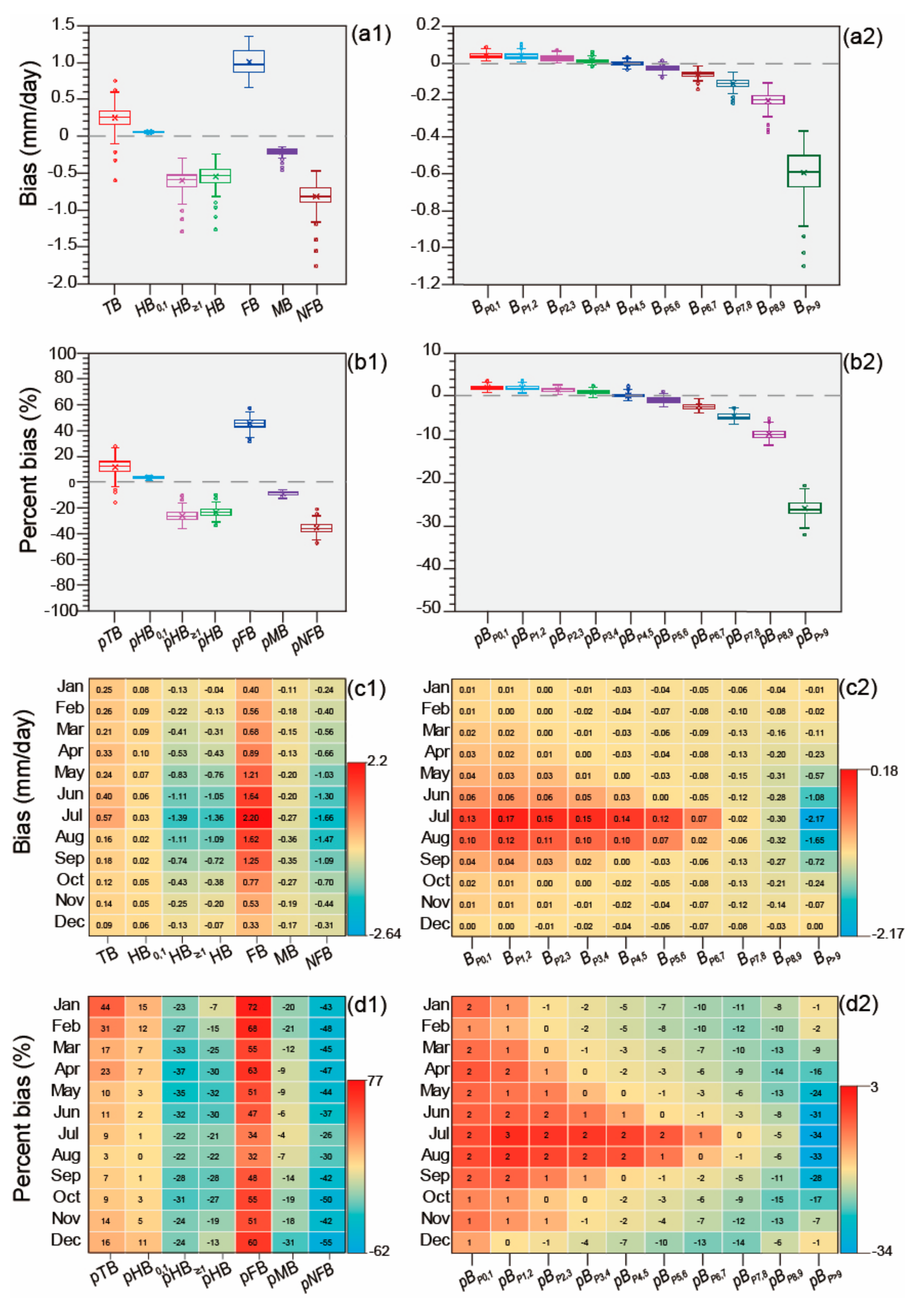
3.2.1. Bias Analyses

Figure 4(a1,b1) reveals that more than 75% of grids show a positive daily TB (pTB), with an HRB mean of 0.25 mm/day (11%), which suggests the overestimation of PERSIANN-CDR on the daily scale across this study region. The values of HB, FB, and MB (Figure 4(a1); pHB, pFB, and pMB, Figure 4(b1)) are always negative, positive, and negative for each grid, respectively, with a regional mean of −0.55, 1.02, and −0.22 mm/day (−24%, 45%, and −10%). Consequently, PERSIANN-CDR daily TB (pTB) can be attributed to larger and positive FB (pFB). To further explore the sources of HB (pHB), we decomposed this metric into two sub-components, i.e., HB0-1 (pHB0-1) and HB≥1 (pHB≥1). Positive HB0-1 (pHB0-1) indicates PERSIANN-CDR overestimation for the bin of daily precipitation lower than 1 mm/day, while negative HB≥1 (pHB≥1) suggests PERSIANN-CDR underestimation for the bin of daily precipitation above 1 mm/day. According to the magnitudes of HB0-1 (0.06 mm/day; pHB0-1, 3%) and HB≥1 (−0.61 mm/day; pHB≥1, −27%), negative daily HB is mainly caused by larger underestimations for daily precipitation above 1 mm/day. In Figure 4(a2,b2), the results of percentile-based biases are presented. For the whole HRB and the overwhelming majority of grids, percentile-based biases are positive and below 0.09 mm/day (4%) between P0 and P4. After P4, biases become negative, and magnitudes and spatial variability become larger as percentiles increase. These findings suggest that PERSIANN-CDR overestimates low daily precipitation, while high daily precipitation is underestimated, especially for precipitation above P8, with biases lower than −0.20 mm/day (−5%).
Figure 4(c1,d1) illustrates the intra-annual cycles of daily biases and detection-based sub-components. Positive values of TB (pTB) represent PERSIANN-CDR overestimations throughout the year. Larger TB values (> 0.20 mm/day) are found between January and July, especially in June and July, with a maximum of >0.40 mm/day, while lower TB (< 0.20 mm/day) occurs in the remaining months (Figure 4(c1)). For the detection-based sub-components for each month, HB, FB, and MB are negative, positive, and negative, respectively, corresponding to larger magnitudes of above 0.70, 1.20, and 0.20 mm/day between May and September. Despite the same signs (i.e., positive and negative), the characteristics of intra-annual cycles of pTB and its sub-components evidently differ from those of TB (Figure 4(d1)), mainly because of apparent differences in daily precipitation magnitudes among months (Figure 2(a1)). For example, pTB is characterized by larger values (>15%) in January–April and December and lower values (<15%) in the other seven months, with the maximum (44%) and minimum (3%) occurring in January and August, respectively. The pFB values in January–May and October–December are above 50%, while pHB (pMB) exhibit magnitudes larger than 30% (10%) in April–June (January–March and September–December). Comparison of HB, FB, and MB (Figure 4(c1); pHB, pFB, and pMB, Figure 4(d1)) indicates that the positive false biases are responsible for the overestimation of PERSIANN-CDR daily precipitation in each month. Throughout the year, HB0-1 (pHB0-1), always with a positive value below 0.10 mm/day (15%), indicates that the PERSIANN-CDR product overestimates daily precipitation below 1 mm/day, but daily precipitation above 1 mm/day is underestimated. This can be seen from negative HB≥1 (pHB≥1) ranging between −1.39 mm/day (−37%) and −0.13 mm/day (−22%). As shown in Figure 4(c2,d2)), PERSIANN-CDR overestimates daily precipitation below P4 for more than six months, with biases larger than 0.10 mm/day (around 2%) in July and August. Conversely, negative biases of daily precipitation above P4 are found in most (> 6) months, and there is a larger magnitude above 0.24 mm/day or 16% (below 0.16 mm/day or 14%) for daily precipitation larger than P9 (between P6 and P8) between April–October (other months). In general, the negative daily non-false biases of the PERSIANN-CDR product in each month are due to its underestimation of higher precipitation.

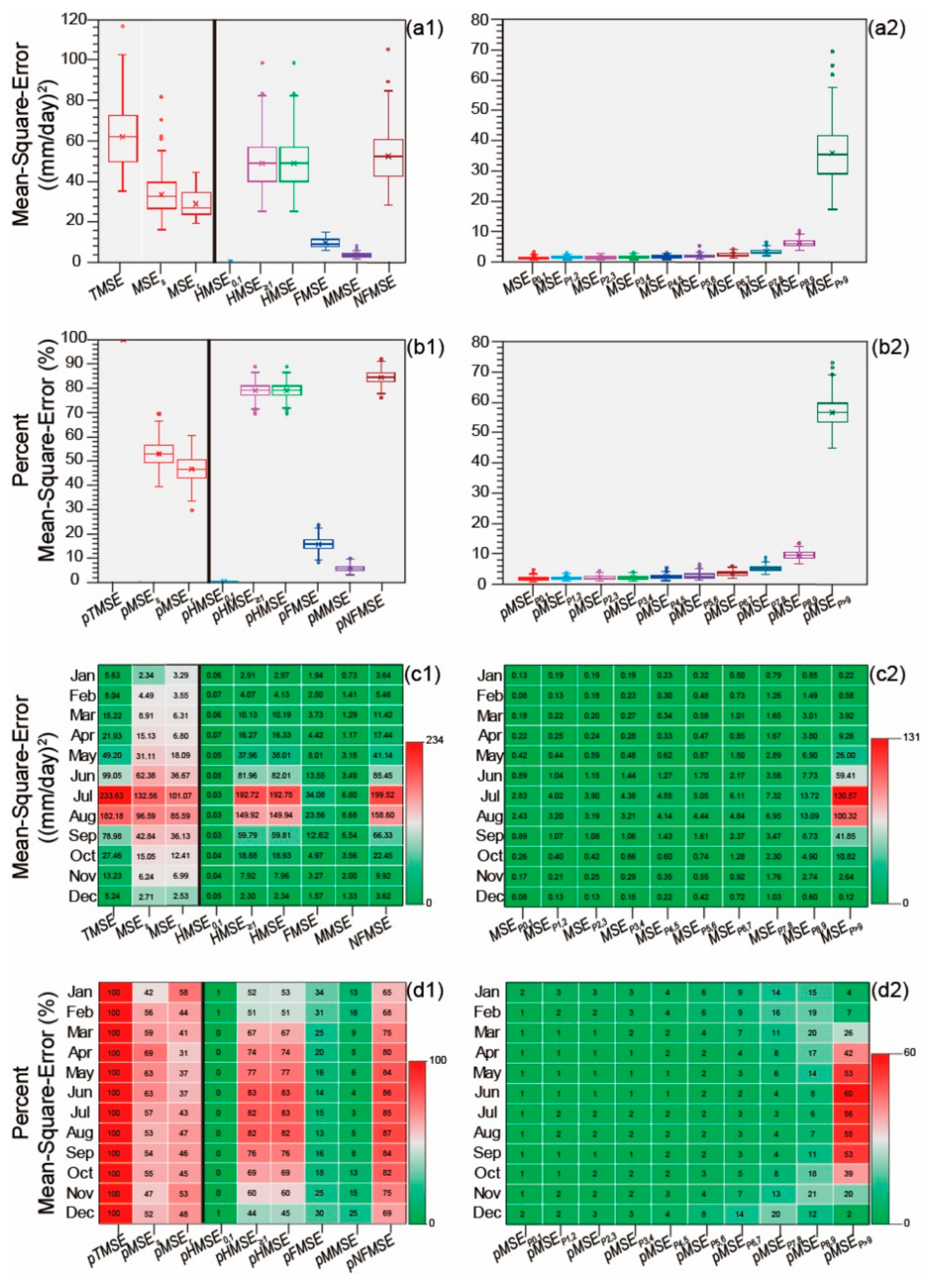
3.2.2. Error Analyses

Figure 5 presents the results of error analyses using daily data. As depicted in Figure 5(a1), TMSE ranges from 35 to 73 (mm/day)2 at half of the grids, with a regional mean of 62.14 (mm/day)2. For the systematic and random error sub-components (left of Figure 5(a1,b1)), MSEs (33.41 (mm/day)2; pMSEs, 53%) is slightly larger than MSEr (28.73 (mm/day)2; pMSEr, 47%). From the perspective of detection-based error sub-components (right of Figure 5(a1,b1)), HMSE (pHMSE) makes the largest contribution of 49.19 (mm/day)2 (79%) to TMSE (pTMSE), followed by the secondary contributor, FMSE (pFMSE), with a value of 9.58 (mm/day)2 (16%). In addition, the HMSE0-1 (pHMSE0-1) value is negligible, while the HMSE≥1 (pHMSE≥1) value is comparable to HMSE (pHMSE), suggesting that the PERSIANN-CDR error is caused by the larger error of precipitation estimates above 1 mm/day. As seen in Figure 5(a2,b2)), the percentile-based error increases as percentiles increase, and is generally characterized by lower values (< 10 (mm/day)2; < 10%) below P9 and a maximum of 35.53 (mm/day)2 (57%) above P9.
Figure 5(c1) shows that the TMSE and its systematic and random sub-components, as well as detection-based error exhibit seasonality. They increase from January, peak in July, and then decrease. Although there exists seasonality for pMSEs and pMSEr (left of Figure 5(d1)), their major characteristics markedly different from those of the TMSE, i.e., larger pMSEs (> 60%) in April–June, but larger pMSEr (> 40%) in January–March and August–December. The pHMSE shows an intra-annual cycle similar to the TMSE, but with a maximum of 83% in June (right of Figure 5(c1,d1)), while pFMSE (pMMSE) values above 20% (10%) are detected in January–April, November, and December (January, February, and October–December). Except for in November, MSEs (pMSEs) always contributes more to the error. Comparisons among the detection-based error sub-components for each month suggest that the largest error proportions exist in HMSE (pHMSE) because of the largest error of PERSIANN-CDR estimations of daily precipitation above 1 mm/day. Between March and October (Figure 5(c2,d2)), the percentile-based error sub-components become larger as percentile increases; however, in the following four months, these variables first increase and then decrease, with the maximum arising between P7 and P9.

3.2.3. R and KGE Analyses

Rall (calculated using all data) values are generally between 0.48 and 0.59 at the overwhelming majority of grids, and the HRB mean is 0.54 (Figure 6(a1)). This suggests that the PERSIANN-CDR product can generally capture the temporal variability of daily precipitation across this region. Excluding non-rainfall data points, we find that the values of R (i.e., R>0 and R≥1, which are estimated using data with OBS daily precipitation of >0 and >1 mm/day, respectively) are comparable to Rall, implying that the effects of these non-rainfall samples have limited impact on R-based performance of the PERSIANN-CDR product on the daily scale. Also, we calculated R between OBS and PERSIANN-CDR (Figure 6(b1)) using samples above given OBS percentiles (i.e., P0, …, and P9). It is evident that as the percentile threshold increases, R decreases, and its spread between the maximum (or the third quantile) and the minimum (or the first quantile) values widens. These results indicate that the ability of PERSIANN-CDR to represent the temporal variability of higher daily precipitation is relatively lower and exhibits larger spatial differences. Among all of the months (Figure 6(c1)), larger values of Rall (regional mean > 0.45) occur in March–November, with a maximum of 0.58 for the HRB mean in June, while lower values of Rall appear in other three months with a regional mean of around 0.40. With the precipitation threshold above a certain OBS percentile (Figure 6(d1)), the R values of each month using daily data show intra-annual cycles the same as Rall’s, with larger values in March–November. Interestingly, the relationship between R values and percentile thresholds reveals that R in January, May–September, and December decreases with percentile thresholds, but R increases for the other five months.
Figure 6(a2–d2) show the KGE results, which represent PERSIANN-CDR’s overall performance skill. The regional mean KGEall (calculated using all data), KGE>0 (calculated based on data with OBS daily precipitation > 0 mm/day), and KGE≥1 (calculated with OBS daily precipitation > 1 mm/day), are between 0.30 and 0.40, implying that PERSIANN-CDR has a moderate skill in reproducing daily precipitation (Figure 6(a2)). With an increased daily precipitation percentile threshold, the corresponding regional mean KGE decreases; it is lower than 0.20 after P5 and even below 0 after P8 (Figure 6(b2)). In Figure 6(c2), the KGE values are larger than 0.30 in 10 months, particularly in June–August and November, with a value above 0.40. However, PERSIANN-CDR data have KGE values of around 0.30 in February and December and even near 0 in January. The intra-annual cycles of KGE for each percentile threshold (Figure 6(d2)) show characteristics similar to KGEall’s, but with lower magnitudes in each month (excluding January). In January, February, October, November, and December, KGEs for each percentile threshold is always lower than 0.15 and even negative, indicating that PERSIANN-CDR lacks the skills to represent daily precipitation in these months. In March–September, KGEs are generally larger than 0.20 for the lower percentile thresholds, implying that this product has some skills in capturing lower precipitation, but no skills in reproducing higher precipitation.

3.2.4. Rainfall Detection Analyses

To characterize the detection capabilities and limitations of the PERSIANN-CDR product, we calculated POD, FAR, ETS, HK, HSS, and FBI values at given precipitation thresholds. These metrics, together with a function of increasing precipitation thresholds, are very useful for measuring the PERSIANN-CDR algorithm performance for different precipitation rates (Figure 7, [57]). It is evident that, in general, POD linearly decreases with increased precipitation thresholds, followed by good (> 0.50) and poor performance (< 0.50) for lower (< P6) and higher (≥ P6) precipitation values, respectively (Figure 7(a1)). The behavior of FAR (Figure 7(a2)) shows an increase from the lowest threshold (P0), a decrease after P0, and an increase after P7. FAR generally fluctuates within a narrow spread between 0.53 and 0.65, indicating that more than 50% of the precipitation detections for each threshold are incorrect, particularly for low thresholds (< P4). ETS shows that the maximum detection skill (a value of 0.26) is achieved at P5, and the skill is limited for precipitation between P0 and P1 or exceeding P9 (Figure 7(a3)). Comparing Figure 7(a4) with Figure 7(a3) shows that, although HSS has larger values, similar behavior is detected for this categorical metric; i.e., the maximum detection skill (0.41) is found at P5. The values of HK (Figure 7(a5)) at most thresholds are above 0.40, and the maximum of 0.49 is observed at P2. These results suggest that the PERSIANN-CDR estimates can generally discriminate between rainfall events at a given threshold. Performance evaluation using FBI scores are above 2.00 (Figure 7(a6)), indicating an overestimation of precipitation totals in thresholds below P7, especially at the thresholds P0, P1, and P2. By contrast, an FBI of below 1.00 shows an underestimation of precipitation totals in thresholds above P6.
As plotted in Figure 7(b1), the behavior of POD in each month shows a decrease as the precipitation threshold increases. Basically, the PERSIANN-CDR product throughout the year corresponds to good performance for precipitation below P4, particularly in June–August, with POD larger than 0.50 continuing until P7. At a given threshold, the corresponding POD shows obvious seasonality, with a peak always occurring in July. FAR (Figure 7(b2)) indicates that more than 50% of precipitation detections are incorrect at almost all thresholds for each month, particularly for precipitation in January–June and September–December below P7, with FAR values larger than 60%. This metric’s fluctuations in each month are characterized by an initial increase, followed by a decrease, and finally, an increase (except for March–May) with increasing thresholds. The monthly pattern of this categorical indicator is similar to that evaluated using all daily data (Figure 7(b2)). Figure 7(b3) shows that the ETS values are all smaller than 0.30. Moreover, the maxima occurs in June–August and the remaining months correspond to precipitation thresholds above and below P5, respectively. HSS (Figure 7(b4)) values do not exceed 0.50, but in each month, the precipitation threshold corresponding to the largest HSS is different, i.e., P1P4 for January–April and September–December, and P4P6 for May–August. Except in July and August, when HK values are large than 0.50 for precipitation thresholds between P2 and P6 (Figure 7(b5)), this indicator’s values are all below 0.50 for other months. In particular, the HK values for thresholds above P6 (P3) in January–April and September–November (December) and above P8 in the remaining months are lower than 0.30, which suggests poor PERSIANN-CDR performance. Overall, FBI behavior generally shows a decrease with increasing percentiles for each month (Figure 7(b6)). However, different tendencies to underestimate or overestimate precipitation events are found among the percentiles. For example, PERSIANN-CDR generally overestimates precipitation below P4 in January–May and October–December, especially for precipitation below P1, with an FBI larger than 3.00. However, it underestimates other precipitation events, e.g., precipitation above P6 having an FBI of less than 0.50. In June–September, most precipitation events are overestimated by the PERSIANN-CDR product.

3.3. Performance Based on Monthly Data

The monthly data shows that the TB (pTB) values are positive at almost all the sites, with a mean of 7.49 mm/month (11%) in the HRB. Biases for precipitation below P9 (Figure 8(a1,b1)) are positive at the overwhelming majority of or even all the grids, and the regional mean is between 0.69 mm/month (0.5%) and 1.50 mm/month (2%). However, performance for PERSIANN-CDR above P9 is distinct, with negative biases for more than 75% of the sites, and a mean of −3.03 mm/month (−4%) for the HRB. If all monthly data are used, the regional mean TMSE is 1587.04 (mm/month)2. The error increases with increasing percentiles (Figure 9(a1,a2)), followed by smaller (< 150 (mm/month)2 or <10%) and larger (> 150 (mm/month)2 or >10%) values for precipitation below and above P7, respectively. Figure 8(a2,b2) illustrate the intra-annual cycle of biases from monthly data. Positive values of HRB biases indicate that this product overestimates precipitation in each month, and the same is true at more than 75% of the grids in all months (except for August). As depicted in Figure 8(a2,b2)), the regional mean TB (pTB) values are larger than 10 mm/month (20%) in June and July (January–April and December). TMSE, MSEs, and MSEr show obvious seasonality, which apparently increases after January and peak in July, followed by a decrease (Figure 9(b1–b3)). Because of differences in TMSE magnitude among months, the seasonal characteristics of pMSEs (pMSEr) differ from those of MSEs (MSEr) (Figure 9(c1,c2)). Generally, pMSEs (pMSEr) first decreases (increases), then increases (decreases), and finally decreases (increases). For each month, comparison between pMSEs and pMSEr illustrates that, except for June and July (which have larger pMSEs values), the error can be attributed to larger random error sub-components in the remaining ten months, and the largest pMSEr (> 70%) is found in November and December show.
Figure 10(a1) plots changes in R with increasing precipitation thresholds. In general, PERSIANN-CDR well represents the temporal variability of monthly precipitation, with the HRB means higher than 0.50 for all precipitation thresholds. Interestingly, regional mean R values decrease with increasing precipitation percentiles, and this implies that the product’s ability to represent temporal variability is relatively weaker for higher precipitation. The intra-annual cycle of R for monthly data is presented in Figure 10(b1). Obviously, PERSIANN-CDR’s ability to represent the temporal variability of monthly precipitation varies from month to month, i.e., better performance (R = ~0.90) in January–March and October–December compared with April–September (excluding July), for which R is below 0.80. The HRB KGE values (Figure 10(a2)) at the precipitation thresholds below P6 are generally constant (~0.75), and then they sharply decrease, ranging from 0.68 at P7 to 0.37 at P9. These findings indicate a comparable and better overall performance of this product in representing monthly precipitation below P6, but the worst overall performance for monthly precipitation occurs above P9. KGE values vary among months (Figure 10(b2)), with larger values (> 0.60) in March and September–December, moderate values (between 0.60 and 0.50) in February and April–June, and lower values (< 0.50) in January and July.

3.4. Performance Based on Annual Data

Table 4 illustrates the PERSIANN-CDR product performance based on annual data. The annual precipitation estimates are higher than the OBS values at the majority (> 75%) of the grids, with a regional mean TB of 89.87 mm/year or a pTB of 11%. For the systematic and random sub-components of annual errors, the HRB mean MSEs and MSEr (pMSEs and pMSEr) are 19896.57 and 10459.86 (mm/year)2 (61% and 39%), respectively, and the former is always larger than the latter at most (> 78%) grids. This finding indicates that the PERSIANN-CDR error results mainly from the systematic error sub-component on the annual scale. With some exceptions (< 25% of grids), the vast majority of the grids show higher values of annual R (> 0.69; KGE > 0.59), with a regional mean of 0.75 (0.63), which indicates that PERSIANN-CDR data can well reproduce the temporal variability of annual precipitation (i.e., the data has a better overall performance).

4. Discussion

4.1. Uncertainties in the PERSIANN-CDR Product

In this study, we comprehensively evaluated the PERSIANN-CDR precipitation product over the HRB by comparison with direct measurements at 176 grid boxes. It should be noted that this product has some shortcomings that may have various origins, including PERSIANN’s conceptual foundations and specifications, as well as inputs (including datasets for calibrating and running the algorithm and adjusting precipitation estimates). Therefore, we will discuss possible sources of this product’s uncertainties in the following subsections.

4.1.1. Uncertainties from PERSIANN’s Conceptual Foundations and Specifications

Richards and Arkin [73] first reported that convective clouds with cold Tb are more likely to produce rain than clouds with warmer cloud-top temperatures. After that, this finding has become a critical conceptual foundation for estimating precipitation with satellite VIS/IR (e.g., PERSIANN developed by Hsu et al. [39]) and MW data. Tb data from GEO satellites generally has a high sampling frequency (i.e., full globe scans are currently available every 15 min), and is selected to infer the position and cloud-top temperature of cloud masses (and, implicitly, cloud-top height). Connections between cloud-top temperature and surface rainfall rates are established using different ground-based precipitation observations as references. However, Tb data can only reflect the cloud’s bulk properties rather than the sophisticated characteristics of microphysics and morphology, and thus does not always correlate well with rainfall. Therefore, these VIS/IR algorithms lack a strong physical basis and are empirical in nature [28,74,75,76]. For example, an actual precipitating region may not be perfectly consistent with and even be smaller than the cold cloud shield in a precipitating system. Sometimes, no rainfall occurs under the coldest section [28,77,78]. This implies that cold clouds (i.e., lower Tb) are neither a sufficient nor necessary condition for rainfall. In this study, higher FAR values, especially for the heavy precipitation and wintertime precipitation (Figure 7(a2,b2)), could be partly due to PERSIANN mistakes cold, but non-precipitating clouds in precipitating systems [76,79,80,81]. Specifically, in convective storms, the relationship between Tb and precipitation rate varies with spatiotemporal storm evolutions [81]. Heavy precipitation actually appears at the edges of a cloud patch, often with higher Tb values relative to the inner core of this patch. As a result, the precipitation rates estimated using fitted parameters of the relationship between Tb and precipitation rate over the whole precipitation area, may have larger negative biases and larger errors [77,78,82]. Similarly, if fitted parameters are employed throughout a storm’s life cycle, VIS/IR algorithms are likely to frequently underestimate rainfall during the early stages, during which the system is mainly controlled by convective cores at high precipitation rates [81]. PERSIANN indeed extracts some useful precipitation information (i.e., statistics of mean and standard deviation of nearby pixels) from IR images and combines MW calibrators [29], although these processes are not enough to provide complete information about a storm’s spatiotemporal evolutions (e.g., higher Tb values at the edges of a cloud patch and early stages of a storm’s life cycle). The two issues above are possible explanations for the larger underestimations of the daily and monthly HRB precipitation at higher percentiles (Figure 4(a2–d2), Figure 5(a2–d2), Figure 8(a1–b1), and Figure 9(a1,a2)).
In PERSIANN and other VIS/IR algorithms, a few critical physical processes that closely relate to precipitation (e.g., sub-cloud evaporation, cloud types, and topography) are not fully considered, potentially introducing uncertainties to precipitation estimates [3,15,16,28,78,83,84,85,86,87]. Kuligowski et al. [84] found significant false alarm rainfall in the TRMM precipitation product in the central part of the U.S. (dry regions). Their further work suggested that this issue is caused largely by the evaporation of hydrometeors below the cloud base [85]. Because IR images do not directly include information about the evaporation of hydrometeors below the cloud base, sub-cloud evaporation effects on precipitation are likely to be partly responsible for the FAR of the PERSIANN algorithm. Because of the close association of cloud types with rain intensities, their delineations are important for accurately estimating precipitation at different intensities, which has been pointed out by numerous studies [15,16,78,88]. Despite that, recognizing types of clouds, which are related to complex three-dimensional structures of water vapor, is difficult based on only the limited information conveyed by Tb in each pixel. Therefore, uncertainties in VIS/IR-based precipitation estimates can come from incomplete and inaccurate information about cloud types. In addition, topographically caused precipitation and warm precipitation clouds (e.g., stratiform) may result in precipitation over a region, for example, northeastern Brazil [3,87]. Current VIS/IR algorithms scarcely consider the topographical impacts, possibly leading to underestimating warm cloud precipitation.
Besides precipitation regime-related issues, VIS/IR-based precipitation product accuracy is likely to be influenced by algorithms’ specifications. The specifications for PERSIANN-CDR include identification of non-rain events, adjustment of 3-hourly precipitation estimates using monthly weight parameters, aggregation of 3-hourly precipitation estimates into daily values, and so on. A slight problem in the PERSIANN model is that 3-hourly precipitation maps have many noisy pixels, which are generally associated with an observed values of zero, but very small non-zero values from neural network model estimates [4,39]. Undoubtedly, this algorithm shortcoming is bound to impact categorical indexes, e.g., high FAR (Figure 7(a3,b3)). Before data aggregation, PERSIANN 3-hourly precipitation is adjusted using monthly weighted parameters, which are ratios between monthly values of the Global Precipitation Climatology Project (GPCP) and PERSIANN estimates. Because this process does not consider weight fluctuations among days, daily precipitation estimates are impossible to be perfectly adjusted. By contrast, adjusted monthly and annual precipitation values are closer to observations, and this is reflected by PERSIANN-CDR’s better performance (i.e., continuous statistics and KGE) on the monthly and annual scales in the HRB. Aggregation of PERSIANN-CDR 3-hourly precipitation estimates may lead to either good or poor daily performance, which is dependent on whether the uncertainties of the 3-hour estimates in one day are offset or accumulated [8,78,89,90,91,92].

4.1.2. Uncertainties from Inputs

Inputs for PERSIANN-CDR mainly consist of the NCEP Stage IV hourly radar precipitation data used for initially training the PERSIANN model, gridded satellite IR data (GridSat-B1) from the International Satellite Cloud Climatology Project (ISCCP) used for running the established model and estimating precipitation, and monthly GPCP data used for adjusting the preliminary product [29]. First, inherent uncertainties in the source data can be propagated into PERSIANN-CDR precipitation estimates. The NCEP Stage IV data, which is high-resolution Doppler next-generation radars (NEXRADs) merged with hourly rain gauge data over the continental U.S. [29,85], has been evaluated over the past several years (e.g., References [72,93,94]). For instance, Nelson et al. [94] summarized this dataset’s disadvantages, including: (1) Bad rain gauge measurements merged in the radar-based precipitation estimation algorithm, especially for hourly estimates; (2) spatial discontinuities of hourly data, e.g., in the Northwest River Forecast Center (i.e., not available), the coast of South Carolina and Georgia from compositing data in these overlapping regions, as well as some River Forecast Centers (RFC)s because of different algorithms and processes (e.g., identifying bad gauge measurements or radar estimates); and (3) evident underlying issues related to radar-based precipitation estimation (e.g., beam blockage, bright band contamination) in the Stage IV product. The GridSat-B1 IR window (IRWIN) Tb data from 1983 to the present, with spatial and temporal resolutions of 10 km and 3 h, is used to drive the PERSIANN model for estimating precipitation [29]. In the process of producing the GridSat-B1 IRWIN data by merging the ISCCP B1 IR data, three sets of calibration (i.e., on-board calibration, ISCCP inter-calibration, and HIRS (high-resolution IR radiation sounder) inter-calibration) have been conducted to derive a consistent and more accurate radiance dataset in space and time [95,96,97,98]. However, some factors, such as view zenith correction, gaps in coverage, and differences in instrument spectral response functions, can also adversely impact the GridSat-B1 IRWIN data quality and then decrease the accuracy of PERSIANN-CDR precipitation estimates [97,99]. Since GPCP products (including monthly, pentad, and daily merged analysis) were developed, they have been widely evaluated with different reference data and used for various relevant studies across the globe [100,101,102,103,104]. For example, GPCP generally captures the spatial patterns of annual and seasonal precipitation over most of the world, but substantial discrepancies appear in some regions (e.g., equatorial West Africa) as a result of low gauge densities [100]. Meanwhile, larger disagreements in spatial and temporal patterns for inter-annual to decadal variations are observed in South America, Africa, and Australia [101,105].
In addition to the propagation of these inherent uncertainties in the source data, Stage IV and GridSat-B1 data can indirectly influence PERSIANN precipitation estimates. For example, Stage IV data is produced by merging the high-resolution Doppler next-generation radars (NEXRADs) and hourly rain gauge data of the continental U.S. References [93,94] rather than the globe, so its representativeness is limited. PERSIANN calibration parameters with this data may not be reasonably employed to the regions outside the continental U.S., especially for those with different atmospheric circulation systems [8]. The East Asian Monsoon prevails in the HRB, and extrapolation of calibrated parameters potentially leads to the local uncertainties in precipitation estimates. Since the duration of some precipitation events may be less than three hours, not all precipitation events are captured by the PERSIANN preliminary product, whose temporal scale of three hours is determined by the GridSat-B1 IR data. For example, convective rainfall events happen in tens of minutes and disappear in a similar period. Despite a shorter duration and smaller spatial extent, these rainfall events may have larger contributions to precipitation totals on various temporal scales (e.g., References [7,106]). Particularly in summer with unstable atmospheric conditions, convective rainfall events regularly take place regularly and likely result in larger uncertainties of precipitation estimates. As a result, inability to capture the short-period (i.e., <3 h) precipitation processes may be a reason for the larger negative biases at higher precipitation percentiles in our study (Figure 4(a2–d2).

4.2. Uncertainties of Rain Gauge Data

Commonly, rain gauge observations are taken as ground truth values for validating various precipitation products (e.g., radar- and satellite-based) on different temporal and spatial scales across the globe, since they have specific advantages, such as accessibility [7,106] (e.g., simple data acquisition and processing), direct and relatively accurate measurements, and long timespans [107,108,109,110,111]. Nonetheless, there are still uncertainties in gauge data, for instance, the inherent difference between point-scale gauge measurements and areal satellite precipitation, i.e., a point of space in time accumulation vs. a snapshot of time in space aggregation. The spatial resolution of PERSIANN-CDR is 0.5° × 0.5°, over which estimated precipitation is averaged, while the footprint of a gauge is much smaller than the coverage of the PERSIANN-CDR pixel. Given the larger variability of precipitation over a small spatial extent, a sparse gauge network may not detect meso-/microscale weather system-related precipitation (e.g., convective precipitation), so gauge precipitation may be lower in magnitude and occurrence than the ground truth values in a target pixel. Overall, mismatches between representatives of satellite-based and gauge precipitation are likely to have an important effect on the accuracy and precision of qualitative and quantitative assessments of satellite-based precipitation products [4,15,16,111,112,113,114]. Moreover, as suggested in numerous studies (e.g., References [8,37,90,114]), a sufficient number of gauges should be collected for the corresponding pixel to decrease the uncertainties induced by gauge representatives. For example, to estimate areal rainfall (for a pixel of about 200 km2) within 20% of its true value, over 25, around 25, 15, and 4 gauges are necessary at the 15 min, hourly, 3-hourly, and daily scales, respectively [114].
Rain gauges are also subject to measurement uncertainties, which are closely associated with flaws in calibration, wind-related undercatch, and wetting-evaporation losses (e.g., References [24,72,107,109,114,115,116,117,118,119,120,121]). Gauges are calibrated (e.g., tipping-bucket rain gauges calibrated using static (volumetric) and dynamic methods), but measured values still contain uncertainties. Shedekar et al. [116] evaluated the accuracies of precipitation observed by three tipping-bucket rain gauges, which had been calibrated in advance. They found that the three devices still significantly underestimated precipitation when compared with actual rainfall depths, especially for greater rainfall intensities. Due to the impacts of flow deflection and the associated eddies and turbulence around gauges (namely, wind-related undercatch effect), wind generally causes some raindrops (especially smaller ones) to miss the funnel or fall at an inclination, which can influence the catch efficiency of the gauge (e.g., References [115,120,121,122,123]). Finally, uncertainties induced by wind effects are dependent on ambient wind speed, raindrop size distribution, and gauge design. Sieck et al. [122] pointed out that wind-exposed aboveground gauges likely observe less rainfall than collocated buried gauges, with a typical undercatch of 2–10% and sometimes more. Wetting losses, defined as water adhering to the inside walls of the gauge and evaporating (or sublimating) without being recorded, generally cause gauge-recorded precipitation to be lower and vary among gauge configurations (e.g., number of times the gauge is emptied) and precipitation types [119]. For example, wetting loss experiments at a gauge site in Russia reported that the average wetting loss was 0.2 mm per record for rainfall observation, but 0.15 mm per record for both snow and mixed precipitation [124]. Rain gauges are exposed to the atmosphere, within which water is always lost through evaporation (namely, evaporation losses). Magnitudes induced by evaporation losses show evident variations among gauge types, climatic zones, and seasons and are typically between 0.1 and 0.8 mm/day or 0–4% of gauged precipitation [108]. Usually, the aggregate impact caused by influential factors of rain gauge measurements is a net underestimation of precipitation [119]. Yang and Ohata [119] developed a bias-corrected (i.e., the aforementioned gauge measurement uncertainties were generally eliminated) climatological precipitation model over Siberia and concluded that after bias correction the annual precipitation increased by 30–330 mm or 10–65% relative to the gauge measurements. This implies that PERSIANN-CDR performance in the HRB based on TB (Figure 4 and Figure 8, and Table 4) is underestimated for daily, monthly, and annual scales, but that derived from percentile-based bias are underestimated and overestimated for lower and higher percentiles, respectively. Moreover, precipitation measurements have an inhomogeneity issue that is imposed by changes in gauge instruments, station relocation, station environment, etc. [30,67,92,125,126]. These factors can have adverse impacts, especially for climatic studies using long-term time series. In this study, we tried our best to reduce the related uncertainties by removing sites with inhomogeneous observations detected by the Pettitt test (because of a lack of metadata for the selected sites); however, there is no guarantee that no inhomogeneity issue exists in the remaining sites, potentially weakening the confidence level of our results.

5. Conclusions

A comprehensive evaluation of a long-term, continuous, and high spatial resolution satellite-based daily precipitation product (PERSIANN-CDR) during the period 1983 to 2012 is conducted in this study by comparing the estimates with rain gauge measurements over the HRB. A suite of statistical measures and techniques were implemented to characterize the differences and agreements between PERSIANN-CDR estimates and rain gauge observations on different time scales. The conclusions are summarized as follows, with some suggestions for the PERSIANN team in improving algorithms and/or corrections in the future and potential users of the PERSIANN-CDR in the HRB.
  • Climatologic characteristics: Despite the differences in magnitudes between PERSIANN-CDR and OBS in the HRB, PERSIANN-CDR can well reproduce intra-annual cycles and spatial characteristics of climatologic precipitation calculated using all data or non-rainfall data.
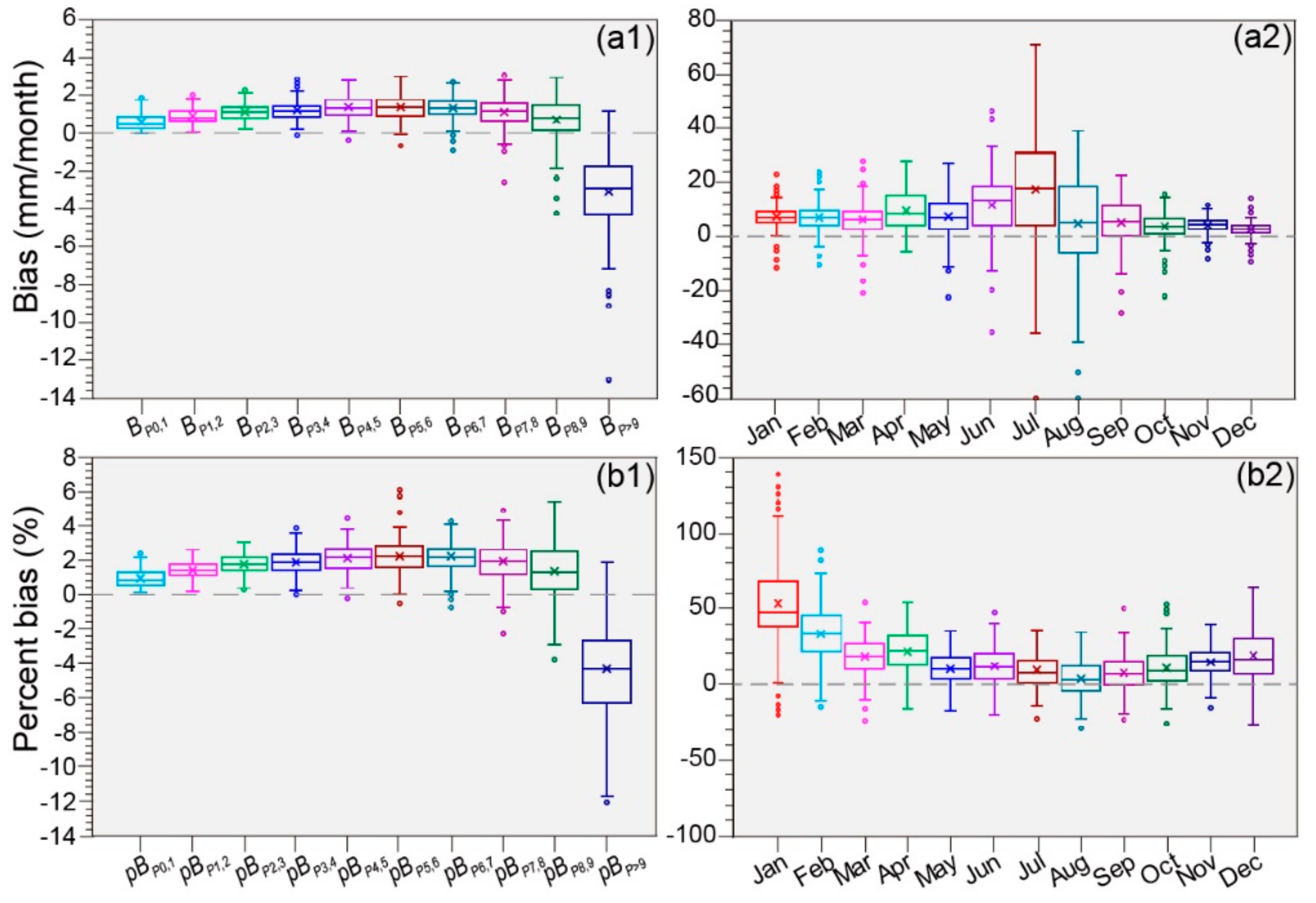
  • Bias analyses: There are daily, monthly, and annual overestimations (with a regional mean pTB of 11%) in the PERSIANN-CDR precipitation data over the HRB. According to detection-based and percentile-based bias compositions, daily overestimations can be attributed to larger and positive FB compared to MB, HB or their sum, followed by negative NFB, which are mainly due to larger underestimations for higher bins. On the monthly scale, overestimations for bins below P9 are likely responsible for larger PERSIANN-CDR estimates; this is also closely associated with daily false biases.
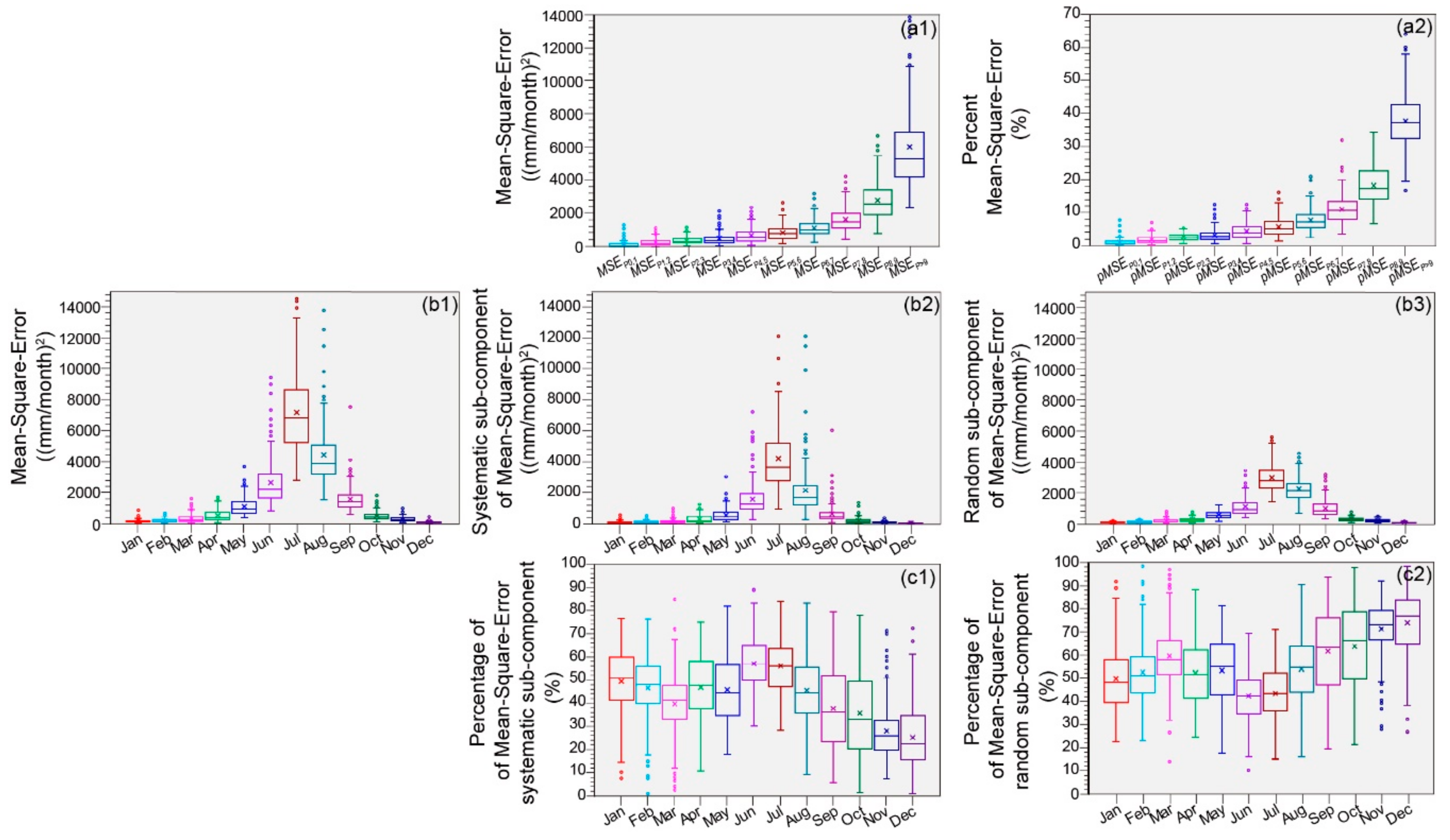
  • Error analyses: Regardless of whether daily, monthly, or annual scales are examined, PERSIANN-CDR errors always come from systematic sub-components of errors. Also, daily and monthly errors are largely the result of larger contributions from errors for bins with higher precipitation.
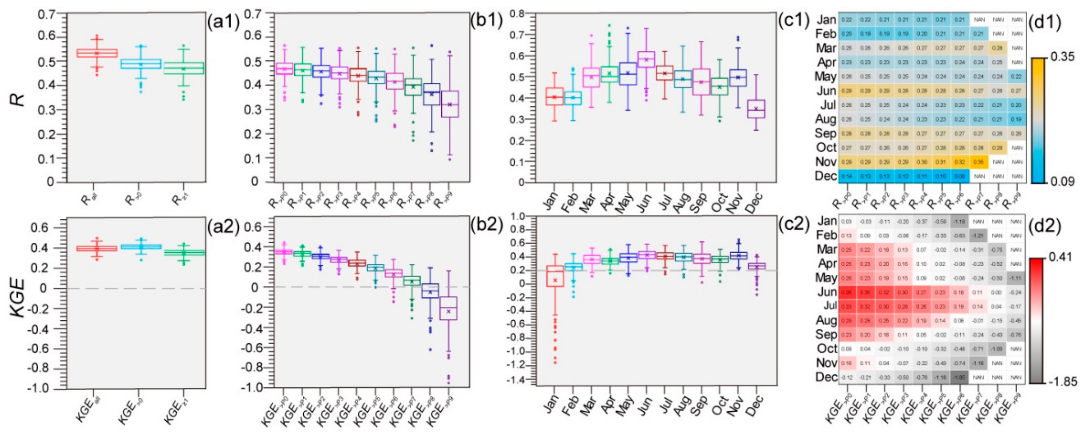
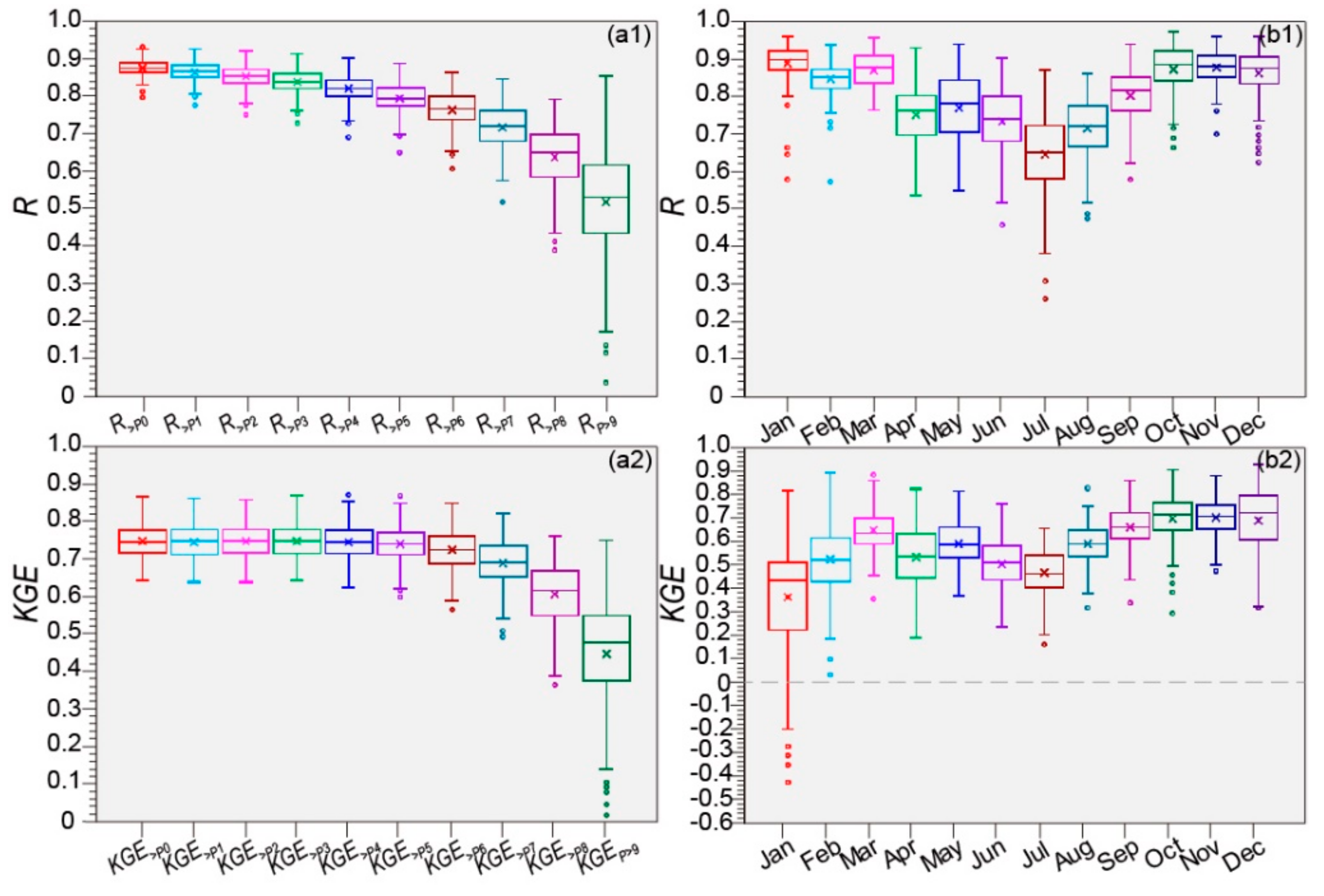
  • R and KGE analyses: For each timescale, R and KGE respectively indicate that PERSIANN-CDR can well capture the temporal variability of precipitation and has a moderate or high overall performance in producing precipitation. Moreover, these capabilities increase from the daily to annual scale, but decrease with the given precipitation thresholds.
  • Detection capability: POD suggests that PERSIANN-CDR has a good (poor) performance in detecting rainfall events with lower (higher) precipitation thresholds. According to FAR for each threshold, this product incorrectly detects more than 50% of precipitation. ETS and HSS both indicate that PERSIANN-CDR has some skill for detecting precipitation between P2 and P8. Based on HK, PERSIANN-CDR can generally discriminate between rainfall events at a given threshold. FBI scores show an overestimation and underestimation of precipitation totals for thresholds below and above P7, respectively.
  • Intra-annual cycles of these validation metrics: Continuous and categorical metrics calculated using daily and monthly data reveal the presence of intra-annual cycles.
Briefly, the comprehensive analyses of PERSIANN-CDR performance in this study provide some significant suggestions for PERSIANN team and the potential users of this precipitation product in the HRB. For example, the analyses of bias and detection capability on various timescales indicate that PERSIANN team can try to develop specific algorithms and/or correction procedures for reducing FB and NFB (especially for rainfall events within higher bins), and thus increasing the overall performance of the PERSIANN-CDR product. The results from error analyses provide a possible solution for the PERSIANN team to decrease PERSIANN-CDR errors, e.g., removing the systematic sub-components using a simple linear regression method established based on the estimates and the observations. Meanwhile, the intra-annual cycles of these selected validation metrics should be involved in the improvements of PERSIANN algorithm and/or correction procedures. For the potential users who focus on the HRB, PERSIANN-CDR can be used for studying water resource from perspectives of intra-annual allocation, spatial distribution, and temporal variability of precipitation, while attention should be paid to the magnitude biases. The relatively poor performance of PERSIANN-CDR at higher precipitation bins indicates that this data has limited capability in capturing heavy rainfall events and potential floods in the HRB. Moreover, this product should be applied with caution for studies related to monthly (seasonal) precipitation, because the intra-annual differences of PERSIANN-CDR performance may cause different uncertainties of the results in each month (season).

Author Contributions

S.S., S.Z. and R.C. conceived and designed this study. S.S., S.Z., H.S., and R.C. were the main authors, whose works included data collection and analysis, interpretation of results, and manuscript preparation. H.C. and G.W. played a supervisory role. R.C., Y.L., W.S., J.W., Y.Z., and H.S. contributed by processing data and providing rain gauge observations. All authors discussed the results and revised the manuscript.

Funding

This work was jointly supported by National Key Research and Development Program of China (Grant No. 2018YFC1507101), Natural Science Foundation of China (Grant Nos. 41605042 and 41875094), Natural Science Foundation of Jiangsu Province, China (Grant No. BK20151525), Qinglan Project of Jiangsu Province of China, Foundation of the Key Laboratory for Cloud Physics and Weather Modification of China Meteorological Administration (Grant No. 2017Z01608) and Foundation of Jiangsu Meteorological Bureau, China (KM201803).

Acknowledgments

PERSIANN-CDR daily precipitation data were downloaded from the Centre for Hydrometeorology and Remote Sensing (CHRS) Data Portal with a website at http://chrsdata.eng.uci.edu, while DEM data of SRTM3 are available from http://srtm.csi.cgiar.org/index.asp. Notably, daily precipitation observations at more than 200 gauge sites are not available to the public, but they can be obtained and used through cooperation with the CMA. We thank all data developers, and their managers and funding agencies, whose work and support were essential for obtaining the datasets, without which the analyses conducted in this study would be impossible. In addition, source codes for conducting this study are available from the authors upon request ([email protected] or [email protected]).

Conflicts of Interest

The authors declare no conflict of interest.

References

  1. GCOS. Implementation plan for the Global Observing System for Climate in Support of the UNFCCC; WMO Tech. Doc. WMO/TD-1523; World Meteorological Organization: Geneva, Switzerland, 2010; p. 186. [Google Scholar]
  2. Kidd, C.; Becker, A.; Huffman, G.J.; Muller, C.L.; Joe, P.; Skofronick-Jackson, G.; Kirschbaum, D.B. So How much of the Earth’s surface is covered by rain gauges? Bull. Am. Meteorol. Soc. 2017, 98, 69–78. [Google Scholar] [CrossRef]
  3. Janowiak, J.E.; Xie, P.; Joyce, R.J.; Chen, M.; Yarosh, Y. Validation of satellite-derived rainfall estimates and numerical model forecasts of precipitation over the United States. In Proceedings of the 29th Annual Climate Diagnostics and Prediction Workshop, Madison, WI, USA, 21–26 October 2004. [Google Scholar]
  4. Grimes, D.I.F.; Coppola, E.; Verdecchia, M.; Visconti, G. A neural network approach to real-time rainfall estimation for Africa using satellite data. J. Hydrometeorol. 2003, 4, 1119–1133. [Google Scholar] [CrossRef]
  5. Thornes, J.; Bloss, W.; Bouzarovski, S.; Cai, X.; Chapman, L.; Clark, J.; Dessai, S.; Du, S.; van der Horst, D.; Kendall, M.; et al. Communicating the value of atmospheric services. Meteorol. Appl. 2010, 17, 243–350. [Google Scholar] [CrossRef]
  6. Sorooshian, S.; AghaKouchak, A.; Arkin, P.; Eylander, J.; Foufoula-Georgiou, E.; Harmon, R.; Hendrickx, J.M.H.; Imam, B.; Kuligowski, R.; Skahill, B.; et al. Advanced concepts on remote sensing of precipitation at multiple scales. Bull. Am. Meteorol. Soc. 2011, 92, 1353–1357. [Google Scholar] [CrossRef]
  7. Wanders, N.; Pan, M.; Wood, E.F. Correction of real-time satellite precipitation with multi-sensor satellite observations of land surface variables. Remote Sens. Environ. 2015, 160, 206–221. [Google Scholar] [CrossRef]
  8. Kidd, C.; Kniveton, D.R.; Todd, M.C.; Bellerby, T.J. Satellite rainfall estimation using combined passive microwave and infrared algorithms. J. Hydrometeorol. 2003, 4, 1088–1104. [Google Scholar] [CrossRef]
  9. Field, C.B.; Barros, V.R.; Dokken, D.J.; Mach, K.J.; Mastrandrea, M.D.; Bilir, T.E.; Chatterjee, M.; Ebi, K.L.; Estrada, Y.O.; Genova, R.C.; et al. (Eds.) IPPC. Summary for policymakers. In Climate Change 2014: Impacts, Adaptation, and Vulnerability. Part a: Global and Sectoral Aspects. Contribution of Working Group II to the Fifth Assessment Report of the Intergovernmental Panel on Climate Change; Cambridge University Press: Cambridge, UK, 2014; pp. 1–32. [Google Scholar]
  10. Trenberth, K.E.; Dai, A.; van der Schrier, G.; Jones, P.D.; Barichivich, J.; Briffa, K.R.; Sheffield, J. Global warming and changes in drought. Nat. Clim. Chang. 2014, 4, 17–22. [Google Scholar] [CrossRef]
  11. Wei, J.; Jin, Q.; Yang, Z.-L.; Dirmeyer, P.A. Role of ocean evaporation in California droughts and floods. Geophys. Res. Lett. 2016, 43, 6554–6562. [Google Scholar] [CrossRef] [Green Version]
  12. Berghuijs, W.R.; Aalbers, E.E.; Larsen, J.R.; Trancoso, R.; Woods, R.A. Recent changes in extreme floods across multiple continents. Environ. Res. Lett. 2017, 12. [Google Scholar] [CrossRef]
  13. Sun, S.; Chen, H.; Ju, W.; Wang, G.; Sun, G.; Huang, J.; Ma, H.; Gao, C.; Hua, W.; Yan, G. On the coupling between precipitation and potential evapotranspiration: Contributions to decadal drought anomalies in the Southwest China. Clim. Dyn. 2017, 48, 3779–3797. [Google Scholar] [CrossRef]
  14. Sun, S.; Li, Q.; Li, J.; Wang, G.; Zhou, S.; Chai, R.; Hua, W.; Deng, P.; Wang, J.; Lou, W. Revisiting the evolution of the 2009–2011 meteorological drought over Southwest China. J. Hydrol. 2019, 568, 385–402. [Google Scholar] [CrossRef]
  15. Hong, Y.; Adler, R.F.; Hossain, F.; Curtis, S.; Huffman, G.J. A first approach to global runoff simulation using satellite rainfall estimation. Water Resour. Res. 2007, 43. [Google Scholar] [CrossRef]
  16. Hong, Y.; Gochis, D.; Cheng, J.; Hsu, K.; Sorooshian, S. Evaluation of PERSIANN-CCS rainfall measurement using the NAME event rain gauge network. J. Hydrometeorol. 2007, 8, 469–482. [Google Scholar] [CrossRef]
  17. Su, F.G.; Hong, Y.; Lettenmaier, D.P. Evaluation of TRMM multisatellite precipitation analysis (TMPA) and its utility in hydrologic prediction in the La Plata Basin. J. Hydrometeorol. 2008, 9, 622–640. [Google Scholar] [CrossRef]
  18. Pan, M.; Li, H.; Wood, E.F. Assessing the skill of satellite-based precipitation estimates in hydrologic applications. Water Resour. Res. 2010, 46. [Google Scholar] [CrossRef]
  19. Nguyen, P.; Ombadi, M.; Sorooshian, S.; Hsu, K.; AghaKouchak, A.; Braithwaite, D.; Ashouri, H.; Thorstensen, A.R. The PERSIANN family of global satellite precipitation data: A review and evaluation of products. Hydrol. Earth Syst. Sci. 2018, 22, 5801–5816. [Google Scholar] [CrossRef]
  20. Xie, P.; Janowiak, J.E.; Arkin, P.A.; Adler, R.; Gruber, A.; Ferraro, R.; Huffman, G.J.; Curtis, S. GPCP pentad precipitation analyses: An experimental dataset based on gauge observations and satellite estimates. J. Clim. 2003, 16, 2197–2214. [Google Scholar] [CrossRef]
  21. Wang, P.K.; Zhang, D.E. An introduction to some historical governmental weather records of China. Bull. Am. Meteorol. Soc. 1988, 69, 753–758. [Google Scholar] [CrossRef]
  22. Wentz, F.J.; Ricciardulli, L.; Hilburn, K.; Mears, C. How much more rain will global warming bring? Science 2007, 317, 233–235. [Google Scholar] [CrossRef]
  23. Habib, E.; Krajewski, W.F.; Ciach, G.J. Estimation of rainfall interstation correlation. J. Hydrometeorol. 2001, 2, 621–629. [Google Scholar] [CrossRef]
  24. Habib, E.; Krajewski, W.F.; Kruger, A. Sampling errors of tipping-bucket rain gauge measurements. J. Hydrol. Eng. 2001, 6, 159–166. [Google Scholar] [CrossRef]
  25. Solomon, S.; Qin, D.; Manning, M.; Chen, Z.; Marquis, M.; Averyt, K.B.; Tigora, M.; Miller, H.L. (Eds.) Climate Change 2007: The Physical Science Basis; Cambridge University Press: Cambridge, UK, 2007; p. 996. [Google Scholar]
  26. Tustison, B.; Harris, D.; Foufoula-Georgiou, E. Scale issues in verification of precipitation forecasts. J. Geophys. Res. Atmos. 2001, 106, 11775–11784. [Google Scholar] [CrossRef]
  27. Maddox, R.A.; Zhang, J.; Gourley, J.J.; Howard, K.W. Weather radar coverage over the contiguous United States. Weather Forecast. 2002, 17, 927–934. [Google Scholar] [CrossRef]
  28. Joyce, R.J.; Janowiak, J.E.; Arkin, P.A.; Xie, P. CMORPH: A method that produces global precipitation estimates from passive microwave and infrared data at high spatial and temporal resolution. J. Hydrometeorol. 2004, 5, 487–503. [Google Scholar] [CrossRef]
  29. Ashouri, H.; Hsu, K.; Sorooshian, S.; Braithwaite, D.K.; Knapp, K.R.; Cecil, L.D.; Nelson, B.R.; Prat, O.P. PERSIANNCDR: Daily precipitation climate data record from multi-satellite observations for hydrological and climate studies. Bull. Am. Meteorol. Soc. 2015, 96, 69–83. [Google Scholar] [CrossRef]
  30. Michaelides, S.; Levizzani, V.; Anagnostou, E.; Bauer, P.; Kasparis, T.; Lane, J.E. Precipitation: Measurement, Remote Sensing, Climatology and Modeling. Atmos. Res. 2009, 94, 512–533. [Google Scholar] [CrossRef]
  31. Xu, S.-G.; Niu, Z.; Shen, Y. Understanding the dependence of the uncertainty in a satellite precipitation data set on the underlying surface and a correction method based on geographically weighted regression. Int. J. Remote Sens. 2014, 35, 6508–6521. [Google Scholar] [CrossRef]
  32. Prigent, C. Precipitation retrieval from space: An overview. Comptes Rendus Geosci. 2010, 342, 380–389. [Google Scholar] [CrossRef]
  33. Anagnostou, E.N. Overview of overland satellite rainfall estimation for hydro-meteorological applications. Surv. Geophys. 2004, 25, 511–537. [Google Scholar] [CrossRef]
  34. Derin, Y.; Yilmaz, K.K. Evaluation of multiple satellite-based precipitation products over complex topography. J. Hydrometeorol. 2014, 15, 1498–1516. [Google Scholar] [CrossRef]
  35. Maggioni, V.; Sapiano, M.R.P.; Adler, R.F. Estimating uncertainties in high-resolution satellite precipitation products: Systematic or random error? J. Hydrometeorol. 2016, 17, 1119–1129. [Google Scholar] [CrossRef]
  36. Ebert, E.E.; Janowiak, J.E.; Kidd, C. Comparison of near-real-time precipitation estimates from satellite observations and numerical models. Bull. Am. Meteorol. Soc. 2007, 88, 47–64. [Google Scholar] [CrossRef]
  37. Huffman, G.J.; Adler, R.F.; Bolvin, D.T.; Gu, G.; Nelkin, E.J.; Bowman, K.P.; Yong, Y.; Stocker, E.F.; Wolff, D.B. The TRMM Multi-satellite Precipitation Analysis (TMPA): Quasi-global, multi-year, combined-sensor precipitation at fine scales. J. Hydrometeorol. 2007, 8, 38–55. [Google Scholar] [CrossRef]
  38. Xie, P.P.; Xiong., A.Y. A Conceptual model for constructing high-resolution gauge-satellite merged precipitation analyses. J. Geophys. Res. Atmos. 2011, 116. [Google Scholar] [CrossRef]
  39. Hsu, K.; Gao, X.; Soroosh, S.; Gupta, H.V. Precipitation estimation from remotely sensed information using artificial neural networks. J. Hydrometeorol. 1997, 19, 69–85. [Google Scholar] [CrossRef]
  40. Huffman, G.J. README for Accessing Experimental Real-Time TRMM Multi-Satellite Precipitation Analysis (TMPA-RT) Data Sets. In NASA Tech. Doc.; 2015; 12. Available online: ftp://meso-a.gsfc.nasa.gov/pub/trmmdocs/rt/3B4XRT_README.pdf (accessed on 10 June 2019).
  41. Funk, C.C.; Peterson, P.J.; Landsfeld, M.F.; Pedreros, D.H.; Verdin, J.P.; Sukla, S.; Husak, G.J.; Rowland, J.D.; Harrison, L.; Hoell, A.; et al. The climate hazards infrared precipitation with stations—A new enviromental record for monitoring extremes. Sci. Data 2015, 2, 1–21. [Google Scholar] [CrossRef] [PubMed]
  42. Kidd, C.; Levizzani, V. Status of satellite precipitation retrievals. Hydrol. Earth Syst. Sci. 2011, 15, 1109–1116. [Google Scholar] [CrossRef] [Green Version]
  43. Laviola, S.; Levizzani, V.; Cattani, E.; Kidd, C. The 183-WSL fast rain rate retrieval algorithm. Path II: Validation using ground radar measurements. Atmos. Res. 2013, 134, 77–86. [Google Scholar] [CrossRef]
  44. Beck, H.E.; Vergopolan, N.; Pan, M.; Levizzani, V.; van Dijk, A.I.J.M.; Weedon, G.P.; Brocca, L.; Pappenberger, F.; Huffman, G.J.; Wood, E.F. Global-scale evaluation of 22 precipitation datasets using gauge observations and hydrological modeling. Hydrol. Earth Syst. Sci. 2017, 21, 6201–6217. [Google Scholar] [CrossRef] [Green Version]
  45. Lo-Conti, F.; Hsu, K.L.; Noto, V.L.; Sorooshian, S. Evaluation and comparison of Satellite precipitation estimations with reference to a local area in the Mediterranean Sea. Atmos. Res. 2014, 138, 189–204. [Google Scholar] [CrossRef]
  46. Chen, F.; Li, X. Evaluation of IMERG and TRMM 3B43 monthly precipitation products over Mainland China. Remote Sens. 2016, 8, 472. [Google Scholar] [CrossRef]
  47. Hussain, S.; Song, X.; Ren, G.; Hussain, I.; Han, D.; Zaman, M.H. Evaluation of gridded precipitation data in the Hindu Kush-Karakoram-Himalaya mountainous area. Hydrol. Sci. J. 2017, 62, 2393–2405. [Google Scholar] [CrossRef]
  48. Mayor, Y.G.; Tereshchenko, I.; Fonseca-Hernández, M.; Pantoja, D.A.; Montes, J.M. Evaluation of Error in IMERG Precipitation Estimates under Different Topographic Conditions and Temporal Scales over Mexico. Remote Sens. 2017, 9, 503. [Google Scholar] [CrossRef]
  49. Omranian, E.; Sharif, H.O. Evaluation of the Global Precipitation Measurement (GPM) satellite rainfall products over the Lower Colorado River Basin, Texas. J. Am. Water Resour. 2018, 1–17. [Google Scholar] [CrossRef]
  50. Palomino-Ángel, S.; Anaya-Acevedo, J.A.; Botero, B.A. Evaluation of 3B42V7 and IMERG daily-precipitation products for a very high-precipitation region in northwestern South America. Atmos. Res. 2019, 217, 37–48. [Google Scholar] [CrossRef]
  51. Sharifi, E.; Steinacker, R.; Saghafian, B. Multi time-scale evaluation of high-resolution satellite-based precipitation products over northeast of Austria. Atmos. Res. 2018, 206, 46–63. [Google Scholar] [CrossRef]
  52. Zeng, Q.; Wang, Y.; Chen, L.; Wang, Z.; Zhu, H.; Li, B. Inter-comparison and evaluation of remote sensing precipitation products over China from 2005 to 2013. Remote Sens. 2018, 10, 168. [Google Scholar] [CrossRef]
  53. Bai, P.; Liu, X. Evaluation of five satellite-based precipitation products in two gauge-scarce basins on the Tibetan Plateau. Remote Sens. 2018, 10, 1316. [Google Scholar] [CrossRef]
  54. Beck, H.E.; Pan, M.; Roy, T.; Weedon, G.P.; Pappenberger, F.; van Dijk, A.I.J.M.; Huffman, G.J.; Adler, R.F.; Wood, E.F. Daily evaluation of 26 precipitation datasets using Stage-IV gauge-radar data for the CONUS. Hydrol. Earth Syst. Sci. 2019, 23, 207–224. [Google Scholar] [CrossRef] [Green Version]
  55. Sunilkumar, K.; Rao, T.N.; Saikranthi, K.; Rao, M.P. Comprehensive evaluation of multisatellite precipitation estimates over India using gridded rainfall data. J. Geophys. Res. Atmos. 2015, 120, 8987–9005. [Google Scholar] [CrossRef] [Green Version]
  56. Gao, J.; Liu, Y.; Zhang, Y. Evolution of temporal-spatial pattern of grain production and its driving mechanism in Huaihe River. Bull. Soil Water Conserv. 2016, 36, 179–185. [Google Scholar]
  57. Zhan, T.; Li, Z.; Mei, M.; Liu, Q. Role of irrigation in crop yield in Huai River Basin. Zhi Huai 2015, 12, 66–68. [Google Scholar]
  58. Hu, Y.; You, F.; Li, X. The evaluation of the coordinating degree between agricultural production capacity and resource environment in Huaihe Basin. Res. Agric. Mod. 2016, 37, 437–443. [Google Scholar]
  59. Liu, J.; Xu, Z.; Bai, J.; Peng, D.; Ren, M. Assessment and correction of the PERSIANN-CDR product in the Yarlung Zangbo River Basin, China. Remote Sens. 2018, 10, 2031. [Google Scholar] [CrossRef]
  60. Liu, X.; Yang, T.; Hsu, K.; Liu, C.; Sorooshian, S. Evaluating the streamflow simulation capability of PERSIANN-CDR daily rainfall products in two river basins on the Tibetan Plateau. Hydrol. Earth Syst. Sci. 2017, 21, 169–181. [Google Scholar] [CrossRef] [Green Version]
  61. Miao, C.; Ashouri, H.; Hsu, K.-L.; Sorooshian, S.; Duan, Q. Evaluation of the PERSIANN-CDR daily rainfall estimates in capturing the behavior of extreme precipitation events over China. J. Hydrometeorol. 2015, 16, 1387–1396. [Google Scholar] [CrossRef]
  62. Guo, H.; Bao, A.; Liu, T.; Chen, S.; Ndayisaba, F. Evaluation of PERSIANN-CDR for Meteorological Drought Monitoring over China. Remote Sens. 2016, 8, 379. [Google Scholar] [CrossRef]
  63. Ghajarnia, N.; Arasteh, P.D.; Liaghat, M.; Araghinejad, S. Error analysis on PERSIANN precipitation estimations: Case study of Urmia Lake Basin, Iran. J. Hydrol. Eng. 2018, 23. [Google Scholar] [CrossRef]
  64. Hussain, Y.; Satgé, F.; Hussain, M.B.; Martinez-Carvajal, H.; Bonnet, M.-P.; Cárdenas-Soto, M.; Roig, H.L.; Akhter, G. Performance of CMORPH, TMPA, and PERSIANN rainfall datasets over plain, mountainous, and glacial regions of Pakistan. Theor. Appl. Climatol. 2018, 131, 1119–1132. [Google Scholar] [CrossRef]
  65. Ashouri, H.; Nguyen, P.; Thorstensen, A.; Hsu, K.-L.; Sorooshian, S.; Braithwaite, D. Assessing the efficacy of high-resolution satellite-based PERSIANN-CDR precipitation product in simulating streamflow. J. Hydrometeorol. 2016, 17, 2061–2076. [Google Scholar] [CrossRef]
  66. Zhang, W.; Pan, S.; Cao, L.; Cai, X.; Zhang, K.; Xu, Y.; Xu, W. Changes in extreme climate events in eastern China during 1960–2013: A case study of the Huaihe River Basin. Quat. Int. 2015, 380, 22–34. [Google Scholar] [CrossRef]
  67. Wijngaard, J.B.; Tank, A.M.G.K.; Konnen, G.P. Homogeneity of 20th century European daily temperature and precipitation series. Int. J. Climatol. 2003, 23, 679–692. [Google Scholar] [CrossRef]
  68. Katiraie-Boroujerdy, P.S.; Nasrollahi, N.; Hsu, K.-L.; Sorooshian, S. Evaluation of satellite-based precipitation estimation over Iran. J. Arid Environ. 2013, 97, 205–219. [Google Scholar] [CrossRef] [Green Version]
  69. Gupta, H.V.; Kling, H.; Yilmaz, K.K.; Martinez, G.F. Decomposition of the mean squared error and NSE performance criteria: Implications for improving hydrological modelling. J. Hydrol. 2012, 377, 80–91. [Google Scholar] [CrossRef]
  70. Zambrano-Bigiarini, M.; Nauditt, A.; Birkel, C.; Verbist, K.; Ribbe, L. Temporal and spatial evaluation of satellite-based rainfall estimates across the complex topographical and climatic gradients of Chile. Hydrol. Earth Syst. Sci. 2017, 21, 1295–1320. [Google Scholar] [CrossRef] [Green Version]
  71. Habib, E.; Henschke, A.; Adler, R. Evaluation of TMPA satellite-based research and real-time rainfall estimates during six tropical related heavy rainfall events over Louisiana, USA. Atmos. Res. 2009, 94, 373–388. [Google Scholar] [CrossRef]
  72. Habib, E.; Larson, B.F.; Graschel, J. Validation of NEXRAD multisensor precipitation estimates using an experimental dense rain gauge network in south Louisiana. J. Hydrol. 2009, 373, 463–478. [Google Scholar] [CrossRef]
  73. Richards, F.; Arkin, P. On the relationship between satellite-observed cloud cover and precipitation. Mon. Weather Rev. 1981, 109, 1081–1093. [Google Scholar] [CrossRef]
  74. Ebert, E.E.; Manton, M.J.; Arkin, P.A.; Allam, R.J.; Holpin, C.E.; Gruber, A. Results from the GPCP Algorithm Intercomparison Programme. Bull. Am. Meteorol. Soc. 1996, 77, 2875–2887. [Google Scholar] [CrossRef] [Green Version]
  75. Arkin, P.A.; Xie, P. The Global Precipitation Climatology Project: First Algorithm Intercomparison Project. Bull. Am. Meteorol. Soc. 1994, 75, 401–419. [Google Scholar] [CrossRef] [Green Version]
  76. Sapiano, M.R.P.; Arkin, P.A. An intercomparison and validation of high-resolution satellite precipitation estimates with 3-hourly gauge data. J. Hydrometeorol. 2009, 10, 149–166. [Google Scholar] [CrossRef]
  77. Scofield, R.A.; Kuligowski, R.J. Status and outlook of operational satellite precipitation algorithms for extreme-precipitation events. Weather Forecast. 2003, 18, 1037–1051. [Google Scholar] [CrossRef]
  78. Behrangi, A.; Hsu, K.; Imam, B.; Sorooshian, S. Daytime Precipitation estimation using bispectral cloud classification system. J. Appl. Meteorol. Climatol. 2010, 49, 1015–1031. [Google Scholar] [CrossRef]
  79. Nasrollahi, N.; Hsu, K.; Sorooshian, S. An artificial neural network model to reduce false alarms in satellite precipitation products using MODIS and CloudSat observations. J. Hydrometeorol. 2013, 14, 1872–1883. [Google Scholar] [CrossRef]
  80. Todd, M.C.; Kidd, C.; Kniveton, D.; Bellerby, T.J.A. Combined satellite infrared and passive microwave technique for estimation of small-scale rainfall. J. Atmos. Ocean. Technol. 2001, 18, 742–755. [Google Scholar] [CrossRef]
  81. Xu, W.; Adler, R.F.; Wang, N.-Y. Combining satellite infrared and lightning information to estimate warm-season convective and stratiform rainfall. J. Appl. Meteorol. Climatol. 2014, 53, 180–199. [Google Scholar] [CrossRef]
  82. Tao, Y.; Gao, X.; Hsu, K.; Sorooshian, S.; Ihler, A. A Deep Neural Network Modeling Framework to Reduce Bias in Satellite Precipitation Products. J. Hydrometeorol. 2016, 17, 931–945. [Google Scholar] [CrossRef]
  83. Kuligowski, R.J.; Li, Y.; Hao, Y.; Zhang, Y. Improvements to the GOES-R Rainfall Rate Algorithm. J. Hydrometeorol. 2016, 17, 1693–1704. [Google Scholar] [CrossRef]
  84. Kuligowski, R.J.; Li, Y.; Zhang, Y. Impact of TRMM data on a low-latency, high-resolution precipitation algorithm for flash-flood forecasting. J. Appl. Meteorol. Climatol. 2013, 52, 1379–1393. [Google Scholar] [CrossRef]
  85. Lin, Y.; Mitchell, K.E. The NCEP stage II/IV hourly precipitation analyses: Development and applications. Preprints. In Proceedings of the 19th Conference on Hydrology, San Diego, CA, USA, 9–13 January 2005; Available online: https://ams.confex.com/ams/pdfpapers/83847.pdf (accessed on 3 April 2019).
  86. Petković, V.; Kummerow, C.D.; Randel, D.L.; Pierce, J.R.; Kodros, J.K. Improving the quality of heavy precipitation estimates from satellite passive microwave rainfall retrievals. J. Hydrometeorol. 2018, 19, 69–85. [Google Scholar] [CrossRef]
  87. Vicente, G.A.; Davenport, J.C.; Scofield, R.A. The role of orographic and parallax corrections on real time high resolution satellite rainfall rate distribution. Int. J. Remote Sens. 2002, 23, 221–230. [Google Scholar] [CrossRef]
  88. Hong, Y.; Hsu, K.; Sorooshian, S.; Gao, X. Precipitation estimation from remotely sensed imagery using an artificial neural network cloud classification system. J. Appl. Meteorol. Climatol. 2004, 43, 1834–1852. [Google Scholar] [CrossRef]
  89. Gebremichael, M.; Krajewski, W.F. Effect of temporal sampling on inferred rainfall spatial statistics. J. Appl. Meteorol. 2005, 44, 1626–1633. [Google Scholar] [CrossRef]
  90. Villarini, G.; Krajewski, W.F. Evaluation of the research version TMPA three-hourly 0.25° × 0.25° rainfall estimates over Oklahoma. Geophys. Res. Lett. 2007, 34. [Google Scholar] [CrossRef]
  91. Morbidelli, R.; Saltalippi, C.; Flammini, A.; Cifrodelli, M.; Picciafuoco, T.; Corradini, C.; Casa-Castillo, M.C.; Fowler, H.J.; Wilkinson, S.M. Effect of temporal aggregation on the estimate of annual maximum rainfall depths for the design of hydraulic infrastructure systems. J. Hydrol. 2017, 554, 710–720. [Google Scholar] [CrossRef] [Green Version]
  92. Morbidelli, R.; Saltalippi, C.; Flammini, A.; Corradini, C.; Wilkinson, S.M.; Fowler, H.J. Influence of temporal data aggregation on trend estimation for intense rainfall. Adv. Water Resour. 2018, 122, 304–316. [Google Scholar] [CrossRef]
  93. Fulton, R.A.; Breidenbach, J.P.; Seo, D.J.; Miller, D.A.; O’Bannon, T. The WSR-88D rainfall algorithm. Weather Forecast. 1998, 13, 377–395. [Google Scholar] [CrossRef]
  94. Nelson, B.R.; Prat, O.P.; Seo, D.-J.; Habib, E. Assessment and implications of NCEP Stage IV quantitative precipitation estimates for product intercomparisons. Weather Forecast. 2016, 31, 371–393. [Google Scholar] [CrossRef]
  95. Knapp, K.R. Calibration assessment of ISCCP geostationary infrared observations using HIRS. J. Atmos. Ocean. Technol. 2008, 25, 183–195. [Google Scholar] [CrossRef]
  96. Knapp, K.R. Scientific data stewardship of International Satellite Cloud Climatology Project B1 global geostationary observations. J. Appl. Remote Sens. 2008, 2. [Google Scholar] [CrossRef]
  97. Knapp, K.R. Inter-satellite bias of the high resolution infrared radiation sounder water vapor channel determined using ISCCP B1 data. J. Appl. Remote Sens. 2012, 6. [Google Scholar] [CrossRef]
  98. Knapp, K.R.; Ansari, S.; Bain, C.L.; Bourassa, M.A.; Dickinson, M.J.; Funk, C.; Holms, C.N.; Holmes, C.D.; Huffman, G.J.; Kossin, J.P.; et al. Globally gridded satellite observations for climate studies. Bull. Am. Meteorol. Soc. 2011, 92, 893–907. [Google Scholar] [CrossRef]
  99. Joyce, R.; Janowiak, J.; Huffman, G. Latitudinally and seasonally dependent zenith-angle corrections for geostationary satellite IR brightness temperatures. J. Appl. Meteorol. 2001, 40, 689–703. [Google Scholar] [CrossRef]
  100. Yin, X.G.; Gruber, A.; Arkin, P. Comparison of the GPCP and CMAP merged gauge-satellite monthly precipitation products for the period 1979–2001. J. Hydrometeorol. 2004, 5, 1207–1222. [Google Scholar] [CrossRef]
  101. Juarez, R.I.N.; Li, W.H.; Fu, R.; Fernandes, K.; Cardoso, A.D. Comparison of Precipitation Datasets over the Tropical South American and African Continents. J. Hydrometeorol. 2009, 10, 289–299. [Google Scholar] [CrossRef]
  102. Ma, L.; Zhang, T.; Frauenfeld, O.W.; Ye, B.; Yang, D.; Qin, D. Evaluation of precipitation from the ERA-40, NCEP-1, and NCEP-2 Reanalyses and CMAP-1, CMAP-2, and GPCP-2 with ground-based measurements in China. J. Geophys. Res. Atmos. 2009, 114. [Google Scholar] [CrossRef]
  103. Huang, D.-Q.; Zhu, J.; Zhang, Y.-C.; Huang, Y.; Kuang, X.-Y. Assessment of summer monsoon precipitation derived from five reanalysis datasets over East Asia. Q. J. R. Meteorol. Soc. 2016, 142, 108–119. [Google Scholar] [CrossRef]
  104. Wang, G.; Zhang, P.; Liang, L.; Zhang, S. Evaluation of precipitation from CMORPH, GPCP-2, TRMM 3B43, GPCC, and ITPCAS with ground-based measurements in the Qinling-Daba Mountains, China. PLoS ONE 2017, 10, e0185147. [Google Scholar] [CrossRef]
  105. Simmons, A.J.; Willett, K.M.; Jones, P.D.; Thorne, P.W.; Dee, D.P. Low-frequency variations in surface atmospheric humidity, temperature, and precipitation: Inferences from reanalyses and monthly gridded observational data sets. J. Geophys. Res. Atmos. 2010, 115. [Google Scholar] [CrossRef]
  106. Blamey, R.C.; Reason, C.J.C. The role of mesoscale convective complexes in southern Africa summer rainfall. J. Clim. 2012, 26, 1654–1668. [Google Scholar] [CrossRef]
  107. Habib, E.; Krajewski, W.F.; Nespor, V.; Kruger, A. Numerical simulation studies of rain gauge data correction due to wind effect. J. Geophys. Res. Atmos. 1999, 104, 723–734. [Google Scholar] [CrossRef]
  108. Adam, J.C.; Lettenmaier, D.P. Adjustment of global gridded precipitation for systematic bias. J. Geophys. Res. Atmos. 2003, 108. [Google Scholar] [CrossRef]
  109. Ciach, G.J. Local random errors in tipping-bucket rain gauge measurements. J. Atmos. Ocean. Technol. 2003, 20, 752–759. [Google Scholar] [CrossRef]
  110. Ma, Y.; Zhang, Y.; Yang, D.; Farhan, S.B. Precipitation bias variability versus various gauges under different climatic conditions over the Third Pole Environment (TPE) region. Intent. J. Climatol. 2015, 35, 1201–1211. [Google Scholar] [CrossRef]
  111. Tang, G.; Behrangi, A.; Long, D.; Li, C.; Hong, Y. Accounting for spatiotemporal errors of gauges: A critical step to evaluate gridded precipitation products. J. Hydrol. 2018, 559, 294–306. [Google Scholar] [CrossRef] [Green Version]
  112. Steiner, M.; Smith, J.A.; Burges, S.J.; Alonso, C.V.; Darden, R.W. Effect of bias adjustment and rain gauge data quality control on radar rainfall estimation. Water Resour. Res. 1999, 35, 2487–2503. [Google Scholar] [CrossRef]
  113. Wood, S.J.; Jones, D.A.; Moore, R.J. Accuracy of rainfall measurement for scales of hydrological interest. Hydrol. Earth Syst. Sci. 2000, 4, 531–543. [Google Scholar] [CrossRef] [Green Version]
  114. Villarini, G.; Mandapaka, P.V.; Krajewski, W.F.; Moore, R.J. Rainfall and sampling uncertainties: A rain gauge perspective. J. Geophys. Res. Atmos. 2008, 113. [Google Scholar] [CrossRef]
  115. Pollock, M.D.; O’Donnell, G.; Quinn, P.; Dutton, M.; Black, A.; Wilkinson, M.E.; Colli, M.; Stagnaro, M.; Lanza, L.G.; Lewis, E.; et al. Quantifying and mitigating wind-Induced undercatch in rainfall measurements. Water Resour. Res. 2018, 54, 3863–3875. [Google Scholar] [CrossRef]
  116. Shedekar, V.S.; King, K.W.; Fausey, N.R.; Soboyejo, A.B.O.; Harmel, R.D.; Brown, L.C. Assessment of measurement errors and dynamic calibration methods for three different tipping bucket rain gauges. Atmos. Res. 2016, 178, 445–458. [Google Scholar] [CrossRef]
  117. Rodda, J.C.; Dixon, H. Rainfall measurement revisited. Weather 2012, 67, 131–136. [Google Scholar] [CrossRef] [Green Version]
  118. Gochis, D.J.; Watts, C.J.; Garatuza-Payan, J.; Cesar-Rodriguez, J. Spatial and temporal patterns of precipitation intensity as observed by the NAME event rain gauge network from 2002 to 2004. J. Clim. 2007, 20, 1734–1750. [Google Scholar] [CrossRef]
  119. Yang, D.; Ohata, T. A bias-corrected Siberian regional precipitation climatology. J. Hydrometeorol. 2001, 2, 122–139. [Google Scholar] [CrossRef]
  120. Duchon, C.E.; Essenberg, G.R. Comparative rainfall observations from pit and aboveground rain gauges with and without wind shields. Water Resour. Res. 2001, 37, 3253–3263. [Google Scholar] [CrossRef] [Green Version]
  121. Nešpor, V.; Sevruk, B. Estimation of wind-induced error of rainfall gauge measurements using a numerical simulation. J. Atmos. Ocean. Technol. 1999, 16, 450–464. [Google Scholar] [CrossRef]
  122. Sieck, L.C.; Burges, S.J.; Steiner, M. Challenges in obtaining reliable measurements of point rainfall. Water Resour. Res. 2007, 43. [Google Scholar] [CrossRef]
  123. Chang, M.; Harrison, L. Field assessments on the accuracy of spherical gauges in rainfall measurements. Hydrol. Process. 2005, 19, 403–412. [Google Scholar] [CrossRef]
  124. Groisman, P.Y.; Koknaeva, V.V.; Belokrylova, T.A.; Karl, T.R. Overcoming biases of precipitation measurement: A history of the USSR experience. Bull. Am. Meteorol. Soc. 1991, 72, 1725–1732. [Google Scholar] [CrossRef]
  125. Alexandersson, H. A homogeneity test applied to precipitation data. J. Clim. 1986, 6, 661–675. [Google Scholar] [CrossRef]
  126. Li, Q.; Peng, J.; Shen, Y. Development of China homogenized monthly precipitation dataset during 1900–2009. J. Geogr. Sci. 2012, 22, 579–593. [Google Scholar] [CrossRef]
Figure 1. Location of the Huai River Basin (HRB) with gauge sites and Precipitation Estimation from Remotely Sensed Information using Artificial Neural Networks-Climate Data Record (PERSIANN-CDR) grids. The digital elevation model (DEM) with a spatial resolution of 90 m is available at http://srtm.csi.cgiar.org/.
Remotesensing 11 01805 g001
Figure 2. Intra-annual cycles of multi-year mean daily (a1a3) and monthly precipitation (b1b3) of OBS and PERSIANN-CDR, which are computed with different thresholds of OBS daily precipitation. Red and blue indicate OBS and PERSIANN-CDR, respectively.
Remotesensing 11 01805 g002
Figure 3. Spatial patterns (a1a6,b1b6,c1c6) of multi-year mean daily, monthly, and annual precipitation of OBS and PERSIANN-CDR, which are computed using different thresholds of OBS daily precipitation.
Remotesensing 11 01805 g003
Figure 4. Bias and its sub-components on a daily scale, with their intra-annual cycles. (a1,b1) show detection-based biases, and (a2,b2) show percentile-based sub-components; (c1,c2,d1,d2) suggest intra-annual cycles of detection-based (percentile-based) biases. B = bias, TB = total B, HB = B in successful detections, MB = B, due to rainfall misses, FB = B because of false detections, HB0,1 = HB for rainfall between 0 mm/day and 1 mm/day, HB≥1 = HB for rainfall above 1 mm/day, NFB = HB≥1 + MB, and BPi,i+1 represents B within [Pi, Pi+1). The percentage expressions of these metrics are labelled with a header of “p”.
Remotesensing 11 01805 g004
Figure 5. Error and its sub-components on a daily scale, with their intra-annual cycles. (a1,b1) are for systematic and random error decompositions and detection-based error sub-components, but (a2,b2) show percentile-based error sub-components; (c1,d1) suggest intra-annual cycles of systematic and random error decompositions and detection-based error sub-components. Intra-annual cycles of percentile-based error sub-components are shown in (c2,d2). MSE = Mean-Square-Error, TMSE = total MSE, MSEs = systematic MSE, MSEr = random MSE, HMSE = MSE in successful detections, MMSE = MSE, due to rainfall misses, FMSE = MSE because of false detections, HMSE0,1 = HMSE for rainfall between 0 mm/day and 1 mm/day, HMSE≥1 = HMSE for rainfall above 1 mm/day, NFMSE = HMSE≥1 + MMSE, and MSEPi,i+1 represents MSE within [Pi, Pi+1). The percentage expressions of these metrics are labelled with a header of “p”.
Remotesensing 11 01805 g005
Figure 6. R (KGE) and its values using data above a given OBS daily precipitation threshold and their intra-annual cycles. (a1,b1) illustrates Rall, R>0, and R≥1 (KGEall, KGE>0, and KGE≥1), while (a2,b2) shows R for each percentile threshold; (c1,d1) (c2,d2) are for the intra-annual cycles of R and its values that correspond to each percentile threshold, respectively. NAN in (d1,d2) suggests that the PERSIANN-CDR product at some grids does not have a rainfall event above a given OBS daily precipitation threshold; here, if the number of grids is more than 10, this index is not shown and labeled NAN.
Remotesensing 11 01805 g006
Figure 7. Categorical metrics using different OBS daily precipitation thresholds (a1a6) and their intra-annual fluctuations (b1b6). The metrics with a subscript (i.e., >”x”) represent PERSIANN-CDR product’s capacity in detecting OBS daily precipitation above “x” mm/day. NAN in b1b6 suggests that the PERSIANN-CDR product at some grids does not have rainfall events above a given OBS daily precipitation threshold; here, if the number of grids is more than 10, the index is not shown and labeled NAN.
Remotesensing 11 01805 g007
Figure 8. Percentile-based biases using monthly data (a1,b1) and intra-annual cycles of TB (a2) and pTB (b2). BPi,i+1 represents B within [Pi, Pi+1), and its percentage expression is labelled with a header of “p”.
Remotesensing 11 01805 g008
Figure 9. Percentile-based Mean-Square-Error (a1,a2); intra-annual cycles of Mean-Square-Error (b1) and its systematic and random sub-components (b2,b3,c1,c2), which are calculated using monthly data. MSEPi,i+1 represents Mean-Square-Error within [Pi, Pi+1), with its percentage expression labelled as a header of “p”.
Remotesensing 11 01805 g009
Figure 10. R (a1) and KGE (a2), which are calculated using data above OBS monthly precipitation percentile thresholds, and intra-annual cycles of R (b1) and KGE (b2) estimated with all monthly data.
Remotesensing 11 01805 g010
Table 1. Validation metrics used in this study.
Type of Validation MetricsIndex and FormulaDescription
Continuous metricsTotal bias (TB):
T B = 1 N i = 1 N ( S i O i ) (1a)
Percent TB (pTB):
p T B = B O × 100 % (1b)
This metric measures the average tendency of PERSIANN-CDR precipitation to be larger or smaller than the observation (OBS), and it has an optimal value of 0. Positive and negative indicate overestimation and underestimation, respectively.
Total Mean-Square-Error (TMSE):
T M S E = i = 1 N ( S i O i ) 2 N (2a)
Percent TMSE (pTMSE):
p T M S E = M S E O 2 × 100 % (2b)
For conveniently decomposing error, TMSE is used here. This indicator, which fluctuates between 0 (an optimal value) and +∞, describes the accuracy of precipitation estimates with the same efficiency as Root-Mean-Square-Error [69].
Correlation coefficient (R):
R = i = 1 N [ ( S i S ) ( O i O ) ] i = 1 N ( S i S ) 2 i = 1 N ( O i O ) 2 (3)
R measures the strength of the linear relationship between PERSIANN-CDR and OBS precipitation, with a range between −1 and 1 (a perfect value).
Kling–Gupta Efficiency (KGE; [69]):
K G E = 1 ( 1 R ) 2 + ( 1 α ) 2 + ( 1 β ) 2 (4)
KGE is a relatively new indicator that is used to measure the overall performance of PERSIANN-CDR. KGE can comprehensively reflect the product’s capability of reproducing temporal dynamics (measured by R) and the volume and distribution of precipitation (measured by α and β, respectively). This index ranges between −∞ and 1, of which KGE = 1 implies a perfect overall performance.
Categorical metricsProbability of Detection (POD):
P O D = A A + D (5)
POD gives the fraction of precipitation occurrences that are correctly detected by the PERSIANN-CDR product. It ranges from 0 to an optimal value of 1.
False alarm ratio (FAR):
F A R = C A + C (6)
FAR gives the fraction of events for which PERSIANN-CDR detects precipitation that is not observed. Its ranges are between 0 (a perfect value) and 1.
Equitable Threat Score (ETS):
E T S = A A r A + C + D A r (7)
The ETS metric indicates the fraction of observed and/or estimated events that are correctly predicted, adjusted by the frequency of hits that would be expected to occur simply by random chance. ETS is bounded by −1/3 and 1 (a perfect score). A value of 0 represents no skill, but negative values indicate that the chance estimation of an event is better than that of the selected product [70].
Heidke Skill Score (HSS):
H S S = 2 · ( A · E C · D ) ( A + D ) · ( D + E ) + ( A + C ) · ( C + E ) (8)
HSS, ranging from −∞ to 1 (an optimal score), shows the accuracy of estimates while accounting for matches, due to random chance. A negative value implies that random chance is better than the selected product’s estimates, and a value of 0 means that the product has no skill.
Hanssen–Kuipers Discriminant (HK):
H K = A A + D C C + E (9)
HK measures how well the satellite estimates discriminate between precipitation and no-precipitation events. This metric has a range between −1 and 1, of which a perfect performance and no skill correspond to 1 and 0, respectively.
Frequency Bias Index (FBI):
F B I = A + C A + D (10)
FBI reveals systematic differences between precipitation event frequency in OBS and PERSIANN-CDR. It can indicate whether there is a tendency to underestimate (i.e., FBI < 1) or overestimate (i.e., FBI > 1) precipitation events and ranges from 0 to infinity, with a perfect score of 1.
Note: Si is the PERSIANN-CDR precipitation value of the ith data pair at a given temporal (i.e., daily, monthly, or yearly) scale, and Oi is the OBS value. α = S/O and β = σS/σO, where S and σS (O and σO) are the mean and standard deviation of PERSIANN-CDR precipitation (OBS), respectively. A = number of hits, C = number of false alarms, D = number of misses, E = number of corrective negatives, N = number of data pairs, and Ar = (A + C)∙(A + D)/N represents hits that could occur by chance. The definitions of A, C, D and E can be found in Table 2.
Table 2. Contingency table to compare OBS and PERSIANN-CDR precipitation.
OBS ≥ ThresholdOBS < Threshold
PERSIANN-CDR ≥ thresholdAC
PERSIANN-CDR < thresholdDE
Note: In view of satellite-based precipitation estimates’ higher uncertainties at low precipitation rates, the threshold is usually considered to be between 1 and 2 mm/day. In accordance with Ebert et al. [36] and Lo-Conti et al. [32], the threshold here is specified to be 1 mm/day, below which all estimated precipitation is considered to be 0 or non-rainfall.
Table 3. Multi-year mean daily, monthly, and annual precipitation for the whole HRB.
Temporal ScalePrecipitationPallP>0P≥1
Daily (mm/day)OBS2.21 (10958)9.17 (578)12.76 (502)
PERSIANN-CDR2.456.558.00
Monthly (mm/month)OBS67.2467.2466.45
PERSIANN-CDR74.6648.2041.83
Annual (mm/year)OBS806.92806.92797.42
PERSIANN-CDR895.90578.36501.90
Note: Pall values are calculated using all data (including data with rainfall and non-rainfall events), while P>0 (P≥1) are obtained using data corresponding to OBS daily precipitation of >0 mm/day (≥1 mm/day). The values in parentheses refer to the number of selected data samples averaged over the HRB.
Table 4. Values of the continuous validation metrics on an annual scale.
Metrics (Unit)HRB MeanMinimum (First Quartile) to Maximum (Third Quartile)
Total bias (TB; mm/year)89.87−40.68 (56.88) to 218.18 (122.73)
Percent TB (%)11−4 (8) to 26 (15)
Total Mean-Square-Error (TMSE; (mm/year)2)30392.448465.76 (20443.71) to 99465.45 (36944.70)
Systematic MSE (MSEs; (mm/year)2)19896.573232.15 (11306.60) to 85706.00 (25030.18)
Random MSE (MSEr; (mm/year)2)10459.864303.34 (7972.03) to 20790.11 (12918.51)
Percent MSEs (pMSEs; %)6125 (51) to 90 (71)
Percent MSEr (pMSEr; %)3910 (8) to 75 (15)
R0.750.52 (0.29) to 0.91 (0.49)
KGE0.630.46 (0.59) to 0.68 (0.83)

