Coastal Dune Vegetation Mapping Using a Multispectral Sensor Mounted on an UAS


1
School of Surveying and Construction Management, Technological University Dublin, Dublin 2, D08 X622, Ireland
2
Environmental Sustainability & Health Institute, Technological University Dublin, Dublin 2, D08 X622, Ireland
*
Author to whom correspondence should be addressed.
Remote Sens. 2019, 11(15), 1814; https://0-doi-org.brum.beds.ac.uk/10.3390/rs11151814
Submission received: 8 July 2019
/
Revised: 29 July 2019
/
Accepted: 31 July 2019
/
Published: 2 August 2019
Abstract
:Vegetation mapping, identifying the type and distribution of plant species, is important for analysing vegetation dynamics, quantifying spatial patterns of vegetation evolution, analysing the effects of environmental changes and predicting spatial patterns of species diversity. Such analysis can contribute to the development of targeted land management actions that maintain biodiversity and ecological functions. This paper presents a methodology for 3D vegetation mapping of a coastal dune complex using a multispectral camera mounted on an unmanned aerial system with particular reference to the Buckroney dune complex in Co. Wicklow, Ireland. Unmanned aerial systems (UAS), also known as unmanned aerial vehicles (UAV) or drones, have enabled high-resolution and high-accuracy ground-based data to be gathered quickly and easily on-site. The Sequoia multispectral sensor used in this study has green, red, red edge and near-infrared wavebands, and a regular camer with red, green and blue wavebands (RGB camera), to capture both visible and near-infrared (NIR) imagery of the land surface. The workflow of 3D vegetation mapping of the study site included establishing coordinated ground control points, planning the flight mission and camera parameters, acquiring the imagery, processing the image data and performing features classification. The data processing outcomes included an orthomosaic model, a 3D surface model and multispectral imagery of the study site, in the Irish Transverse Mercator (ITM) coordinate system. The planimetric resolution of the RGB sensor-based outcomes was 0.024 m while multispectral sensor-based outcomes had a planimetric resolution of 0.096 m. High-resolution vegetation mapping was successfully generated from these data processing outcomes. There were 235 sample areas (1 m × 1 m) used for the accuracy assessment of the classification of the vegetation mapping. Feature classification was conducted using nine different classification strategies to examine the efficiency of multispectral sensor data for vegetation and contiguous land cover mapping. The nine classification strategies included combinations of spectral bands and vegetation indices. Results show classification accuracies, based on the nine different classification strategies, ranging from 52% to 75%.

1. Introduction
Coastal dune fields are at the transition between terrestrial and marine ecosystems and are highly-valued, natural resources for providing drinking water, mineral resources, recreation, eco-services and desirable land for development [1]. These natural resources provide food and habitation for aquatic and terrestrial organisms and, also, offer human settlement and recreation spaces. Activities at the coastal zone area can contribute to local and national economic development in areas like aquaculture, fisheries and tourism, and the area also has an important function to control erosion and flooding, thus protecting and maintaining environmental functions [2]. In recent years, increasing tourism and development in the coastal dune area in the southeast of Ireland have resulted in increased pressure on the environment, resulting in issues including soil erosion, flooding and habitat loss [3].
Vegetation at coastal dune complexes has a strong impact on dune morphology and dynamics as it can influence sand transport [4]. Vegetation is also a critical environmental component of the coastal ecosystem for food production, resource conservation, nutrient cycling and carbon sequestration [5,6]. High-resolution vegetation mapping of coastal dune complexes, with accurate distribution and population estimates for different functional plant species, can be used to analyse vegetation dynamics, quantify spatial patterns of vegetation evolution, analyse the effects of environmental changes on vegetation and predict spatial patterns of species diversity [7]. Such information can contribute to the development of targeted land management actions that maintain biodiversity and ecological functions.
This research involved the generation of 3D vegetation mapping of a coastal dune complex at Buckroney in Co. Wicklow, Ireland, using a multispectral sensor mounted on an unmanned aerial system (UAS) (Figure 1). The research presents a workflow for 3D vegetation mapping of a coastal dune complex, including establishing ground control points (GCPs), planning the flight mission and camera parameters, acquiring the imagery, processing the image data and performing digital features classification. The process illustrates the efficiency of image data collection and the high-resolution of the vegetation mapping of the site using a multispectral camera mounted on a UAS. Classification accuracy also needs to be considered and some research also quoted an overall classification accuracy of 65% as the minimum acceptable for reliable vegetation mapping [8]. To examine the efficiency of multispectral sensors for vegetation mapping, classification was conducted based on 10 different classification strategies, including different combinations of wavebands and spectral indices.
2. Background
Traditionally, field survey has been the most commonly used method for vegetation mapping [9]. However, this method is time-consuming, expensive and limited in spatial coverage [10]. Satellite remote sensing, in contrast, offers a potentially more efficient means of obtaining data. Each vegetation community has a unique spectral response in multispectral satellite image data which is a function of the characteristic species composition [11,12]. Satellite-based hyperspectral data can be a useful tool for vegetation mapping on a regional scale but, in the context of species level classification, it is limited to homogeneous stands of the same species because of limited spatial resolution (e.g., 30 m of EO1 Hyperion images), and low signal-to-noise ratio [13].
Airborne remote sensing provides higher spatial resolution data than satellite remote sensing for coastal dune complexes mapping and a higher resolution is more suitable for coastal dune inspection and monitoring [14]. Light detection and ranging (LiDAR) is an active remote sensing technique that measures the return time of a laser pulse backscattered by a target as an echo signal whose intensity is proportional to the reflectance properties of the target [15]. Classical LiDAR records discrete echoes in real-time but may not distinguish targets that are too close to each other. The minimum target separation is typically 0.4 m in airborne LiDAR [14]. LiDAR data is often available from national mapping agencies (NMAs), such as Ordnance Survey Ireland (OSi) who quote spatial resolutions and vertical accuracies in rural areas of 0.5 m and 0.5 m, respectively [16]. However, LiDAR data from NMAs are of limited use for vegetation mapping of coastal dune areas because of the relatively coarse spatial resolution, poor vegetation classification potential and fixed acquisition dates.
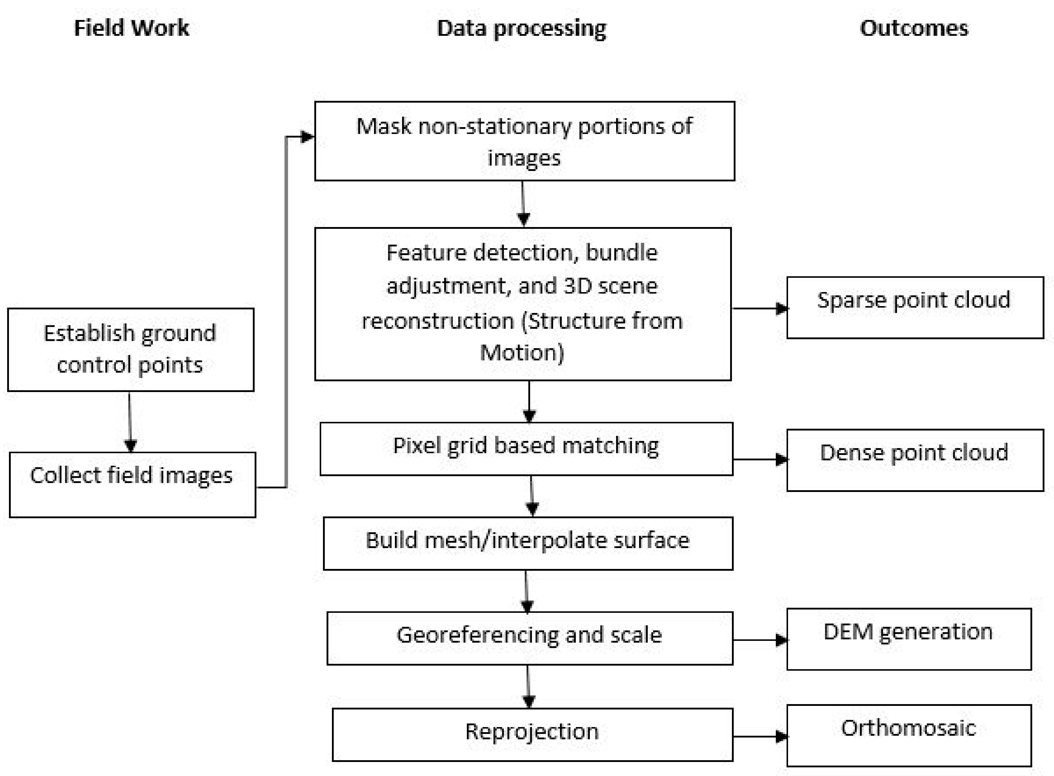
In recent years, there have been significant advances in exploring the capabilities of small UAS (unmanned aerial systems) as part of vegetation research [17,18,19,20]. UAS, variously referred to as remotely piloted aircraft systems (RPAS), unmanned aircraft vehicles (UAV), “Aerial Robots” or simply “drones”, enable on-site data collection for vegetation mapping [21]. In comparison with other remote sensing platforms, UAS typically have a lower operating height which enables the collection of higher spatial resolution in a small area [22]. UAS also have flexible revisit times whereas the availability of other remote sensing data is limited in acquisition date and coverage depending on national commission. UAS also provide the possibility for data acquisition of inaccessible areas or hazardous environments. The collected images are processed by specialized software, for example Pix4D or Agisoft, which utilize structure from motion (SfM) technology and dense image matching. Importing a wide variety of suitable imagery and control data to the software, a georeferenced 3D model can be constructed. Figure 2 shows a workflow for photogrammetry-based 3D construction based on Bemis’s research [23].
Structure from motion (SfM) for UAS-collected data processing is a technique that has emerged in the last decade to construct photogrammetry-based 3D models [24]. The critical element for implementation of photogrammetry to 3D mapping using SfM is the collection of numerous overlapping images of the study area [25]. From each pair of overlapping pictures, SfM can calculate the unique coordinate position (x, y, z or easting, northing, elevation) of a set of particular points presented in both images. To maintain the accuracy of the mapping, the overlapping area for each two images should be at least 60%, ensuring that sufficient shared points can be recognised by software for the map construction. To generate a 3D model, many thousands of matching object and textural features are automatically detected in multiple overlapping images of the ground surface, from which a high-density point cloud with 3D coordinate positions is derived.
A multispectral camera mounted on a UAS allows both visible and multispectral imagery to be captured that can be used for characterizing land features, vegetation health and function. The Parrot Sequoia multispectral sensor has green (530–570 nm), red (640–680 nm), red edge (730–740 nm) and near-infrared (770–810 nm) wavebands and a camera with red, green and blue wavebands (RGB camera) (400–700 nm) [26]. Colour, structure and surface texture of different land features can influence the reflectance pattern of the wavebands [27]. By analysing these spectral reflectance patterns, different earth surface features can be identified. This process is known as classification and it is usually carried out by digital image processing using a variety of classification algorithms.
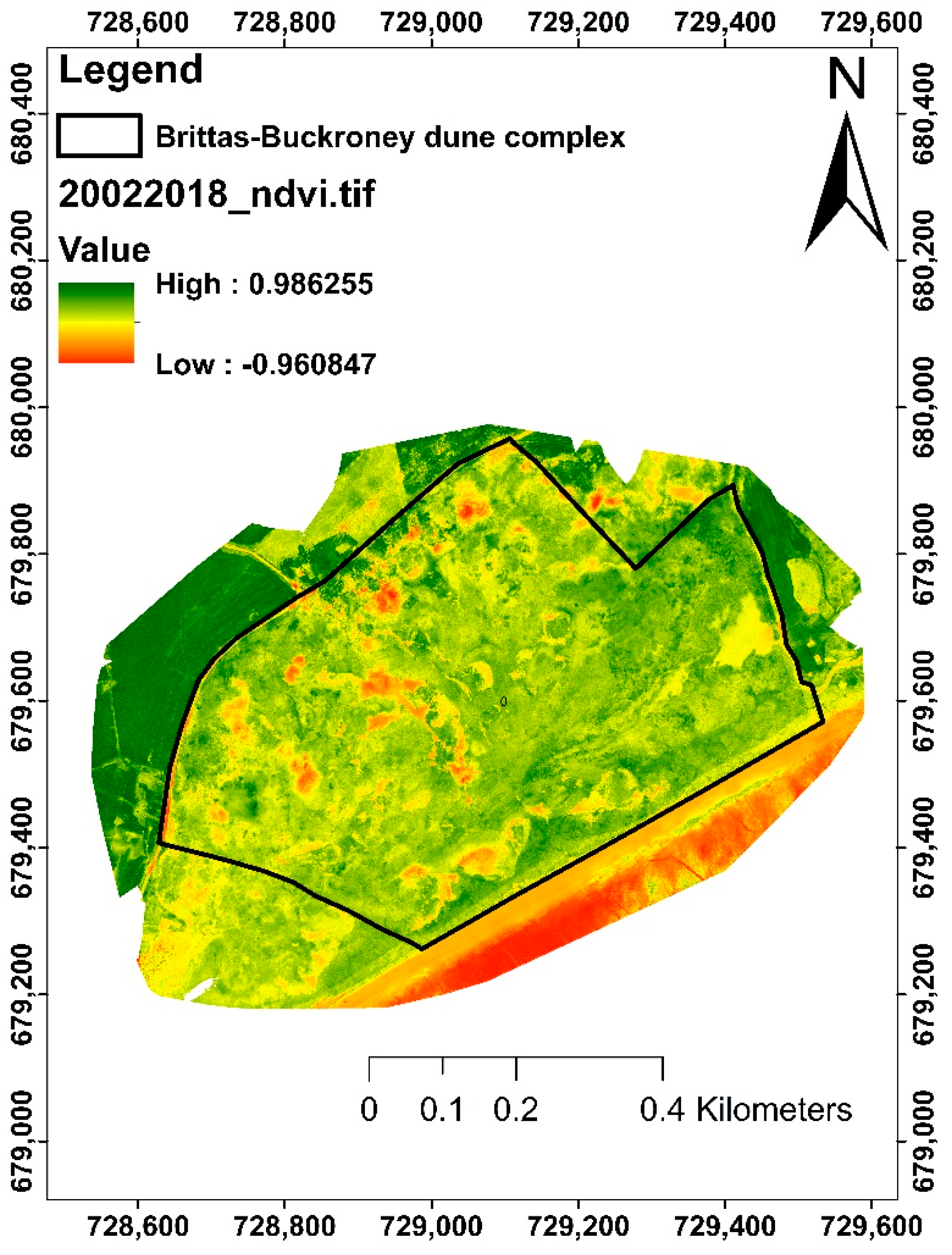
Image processing is also capable of discriminating vegetation by calculating different visible-based or multispectral data-based spectral indices. For example, the Normalized Differential Vegetation Index (NDVI), which relates the reflectance of land features at near-infrared and red wavebands, is widely used to differentiate green vegetation areas from other land features, such as water and soil [28]. The index ranges from −1 to 1, with 0 representing the approximate value of no vegetation [29]. There are other spectral indices that can be calculated from multispectral bands and are used for vegetation mapping, Weil et al. listed six of these related with RGB camera-based bands and four multispectral bands (Table 1) [20].
Overhead imagery of natural terrain typically includes shading and weaker reflectance from shaded areas complicates the classification of vegetation communities. Various image pre-processing methods have been developed to minimize the effects of shadows on image classification. These methods include band ratios (e.g., [30,31]), additional topographic data (e.g., [32]) and topographic correction (e.g., [33,34]). Band ratios can minimize changes in solar illumination caused by variations in slope and aspect [35]. Research has also demonstrated that simulated NDVI is resistant to topographic effects at all illumination angles [36]. The normalized difference moisture index (NDMI) and tasselled cap wetness have also been used to classify forest types [37]. The use of digital elevation models (DEM) in vegetation classification in mountainous regions has also proven useful in improving classification accuracy, if the distribution of vegetation is determined by altitude [38]. Topographic correction models have also been applied to Landsat images and have been shown to increase classification accuracies [39].
3. Study Site
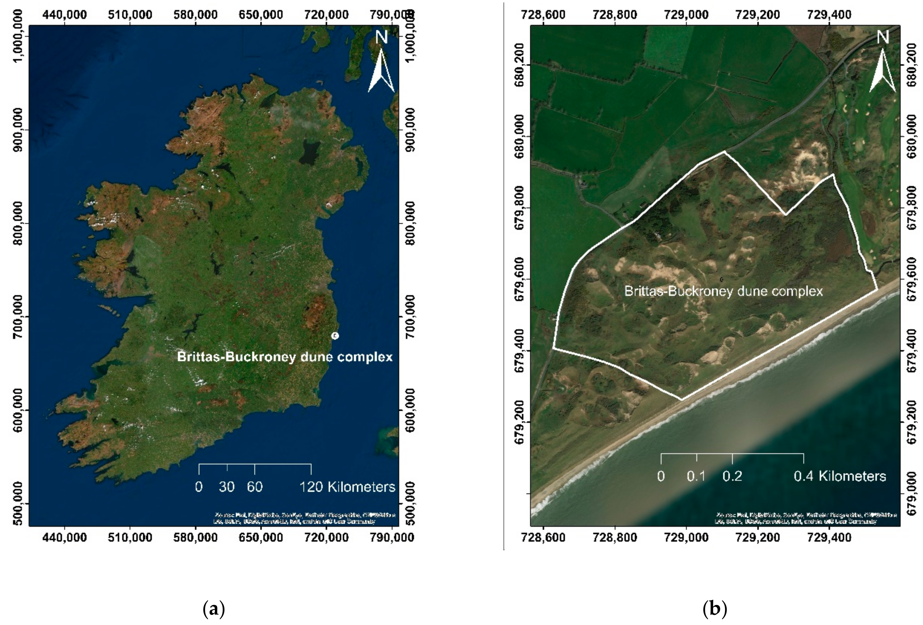
The Brittas-Buckroney dune complex (Figure 3) is located c. 10 km south of Wicklow town on the east coast of Ireland and comprises two main sand dune systems, viz. Brittas Bay and Buckroney Dunes [8]. The study site for this research is Buckroney Dunes, which is managed by the Irish National Park and Wildlife Service. The area of the Buckroney dune complex is c. 40 ha. Within this site, ten habitats listed on the European Union (EU) Habitats Directive are present, including two priority habitats in Ireland, viz. fixed dune and decalcified dune heath [40]. This dune system also contains good examples of other dune types. At the northern part of Buckroney dune complex, there are some representative parabolic dunes, while embryonic dunes mostly occur at the southern part.
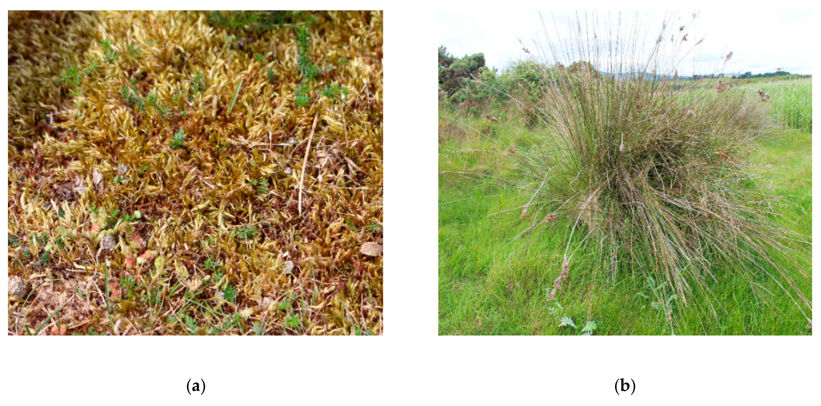
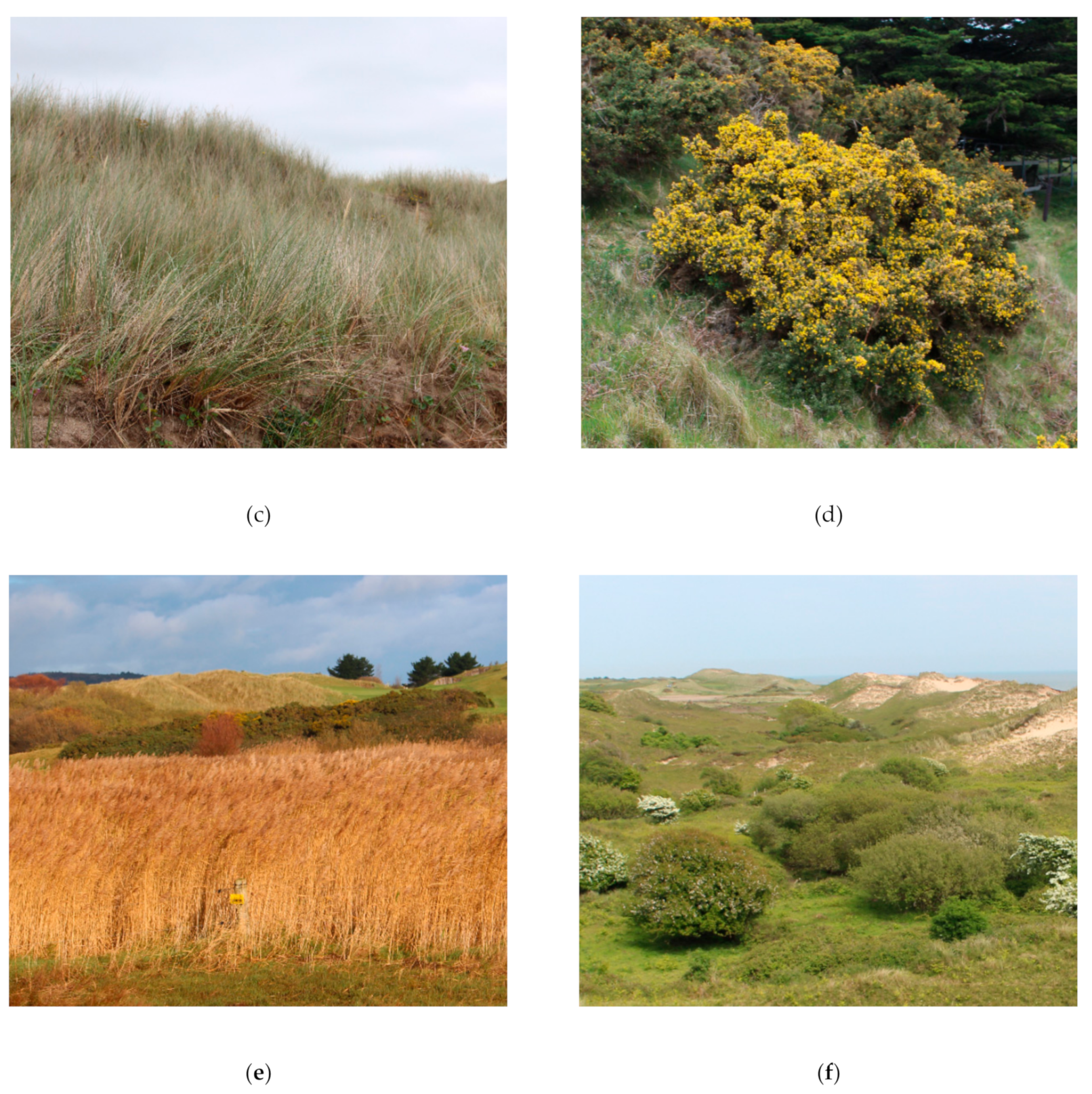
The site is notable for the presence of well-developed plant communities as shown in Figure 4 [39]. Mosses, such as Tortula ruraliformis (Syntrichia ruralis subsp. ruraliformis), Rhytidiadelphus triquetris, and Homalothecium lutescens and lichens (Cladonia spp., Peltigera canina), are frequently found in this dune complex. Sharp rush (Juncus acutus L.) dominates south of the inlet stream to the fen area at the north of the dune complexes, and in small areas elsewhere within the Buckroney dune complex. The main dune ridges are dominated by European marram grass (Ammophila arenaria (L.) Link). Gorse (Ulex europaeus (L.)) is also present at the back of the dunes. To the west, a dense swamp of common reed (Phragmites australis (Cav.) Trin. ex Steud.) is present. There are also extensive areas of rusty willow (Salix cinerea subsp. oleifolia Macreight) scrub throughout the dune complex.
With land acquisition in recent years, the marginal areas of the dune system have been reclaimed as farmland. The increasing anthropogenic activities at the dune system, such as farming and recreation activities, have brought pressure on the development of the dune ecosystem, with hazards like soil erosion, flooding and habitat loss. Accurate and high-resolution 3D vegetation mapping can contribute to an understanding of the natural processes that impact the coastal dune complex and can help with the development of targeted land management policies.
4. Methodology
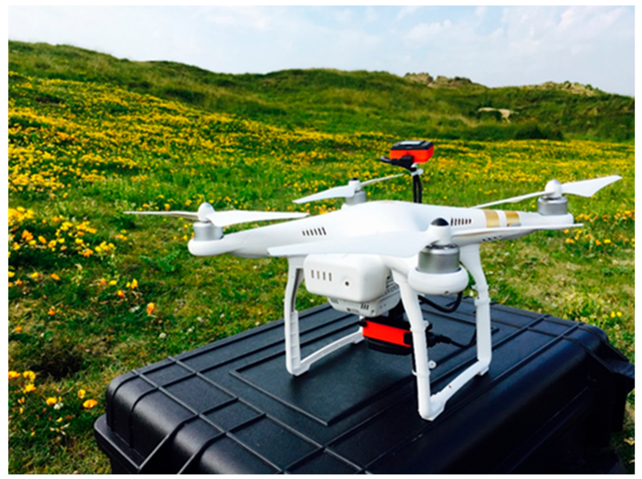
The UAS platform used was a DJI Phantom 3 Professional (Shenzhen, Guangdong, China), which has four rotors, a central body containing the electronic components and landing gear that sustains the entire structure (Figure 5). The UAS is powered by a lithium polymer battery that allows a flight time up to 25 min. The multispectral sensor used in this study was a Parrot Sequoia which is comprised of five individual cameras and a sun sensor. The cameras consist of a 16 MP RGB camera and four 1.2 MP multispectral cameras that record in green, red, red edge and near-infrared wavebands. The camera cluster is mounted under the central body of the UAS and a sun sensor is positioned above the central body as seen in Figure 5. The field work for this study was conducted in February 2018.
4.1. Field Work
4.1.1. Ground Control Points
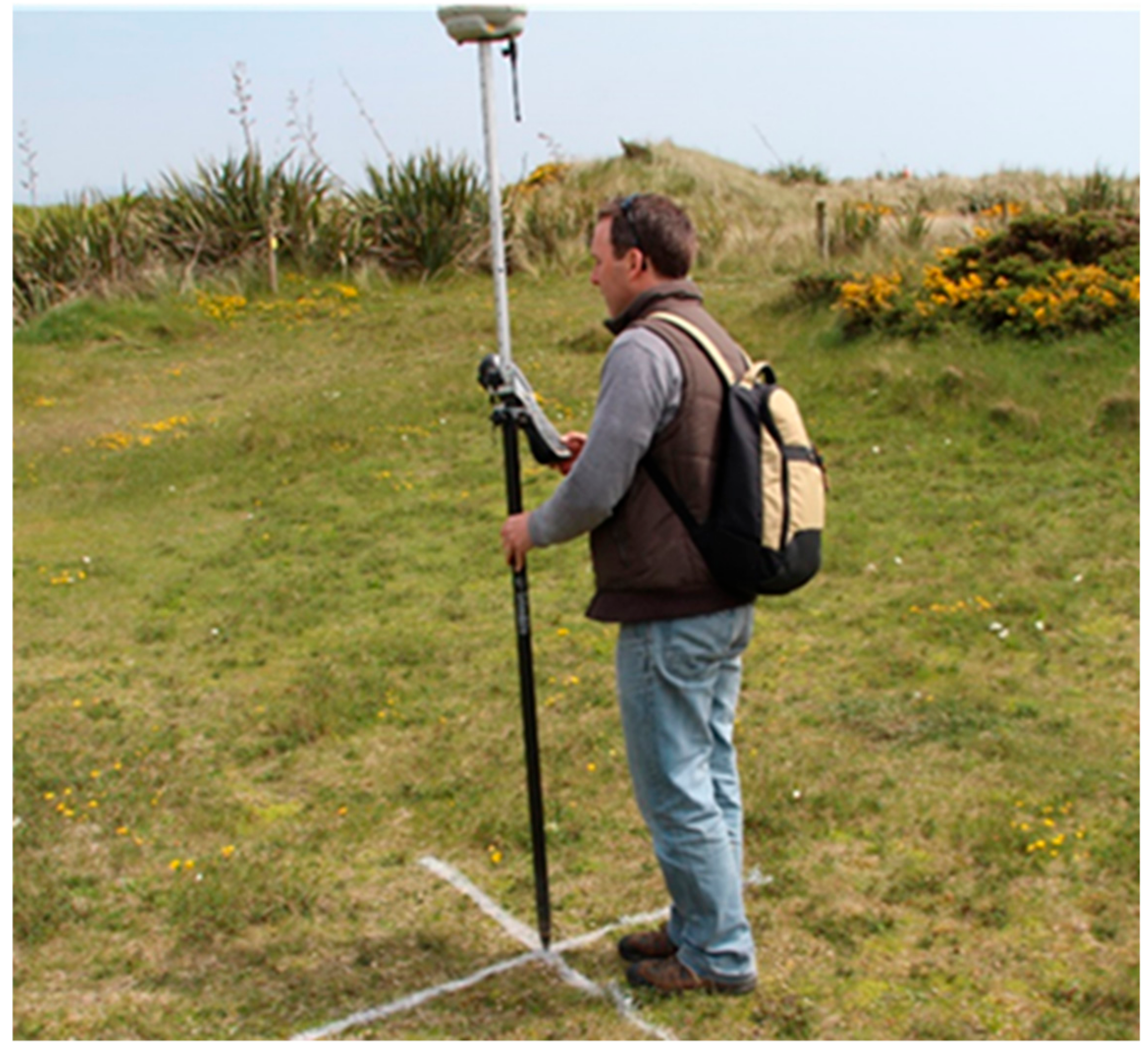
Field surveying with the UAS started with establishing ground control points (GCPs) across the study site whose Irish Transverse Mercator (ITM) coordinates were determined using a Trimble Global Navigation Satellite System (GNSS) receiver connected to the Trimble Virtual Reference Station (VRS) Network Real Time Kinematic (NRTK) system (Figure 6). This system can reach 2 cm spatial and 5 cm vertical accuracy for point measurement [41]. These GCPs were used at the processing stage to georeference the 3D models generated from the data. In this study, 20 GCPs, marked as white crosses on-site, were recorded. To ensure visibility in the captured images, open, flat and relatively bare ground locations were selected for the GCPs.
4.1.2. Flight Mission Planning
Pix4DCapture (Prilly, Switzerland) software provided a solution for the flightpath design for the UAS surveying project while separate Parrot Sequoia software was used to set the multispectral sensor recording parameters. For this study, the parameters of the flight mission were set as shown in Table 2 and Table 3.
4.1.3. Radiometric Calibration
Radiometric calibration was required to convert the multispectral raw imagery data to absolute surface reflectance data thereby removing the influence of different flights, dates and weather conditions. A collection of solar irradiance data for each flight is required for radiometric calibration. Imaging of a white balance card (Figure 7), captured before each flight, provided an accurate representation of the amount of light reaching the ground at the time of capture. The balance card containing a grey square and Quick Response (QR) codes around it. The large grey square in the centre of the balance card is a calibrated “panel” that can be used to calibrate the reflectance values as every balance card has been tested to determine its reflectance across the spectrum of light captured. The captured balance card images provided absolute reference information which was applied to each image individually for the collection of repeatable reflectance data over different flights, dates and weather conditions.
4.1.4. Other Considerations
After setting the flight parameters and reflectance calibration, a number of other items were considered before launching the UAS to ensure a safe and effective flight. These included weather conditions, backup battery, subscriber identification module (SIM) card for image storage and UAS controller charge. In case of an emergency, the flight could be terminated manually from the controller. In consideration of the maximum 25 min battery life for a single flight of the UAS, the study site of about 40 ha was divided into three overlapping flying events.
4.2. Data Processing
Overlapping imagery data collected by the UAS was processed with Pix4D software to generate geo-referenced orthomosaics, digital surface models (DSMs), contours, 3D point clouds and textured mesh models in various formats. As the image database of this research was large, a computer with seven cores (i7), 32 GB of RAM and 1.5 TB storage was used to process and save the files. The procedure is highly automated but required over 70 processing hours for the whole study site. The RGB imagery and multispectral imagery were processed in two separate projects. The RGB project required GCP position information to refer the project in the ITM coordinate system. Images of the calibration target were used for radiometric calibration and to remove the brightness difference in the multispectral bands project. Other processing options were customized to select the proper scale and format for the resulting data. A quality assessment report for each processing step was generated and stored.
4.3. Classification
From the orthomosaic model generated from the captured imagery, areas dominated by plant species, including pasture, rusty willow, gorse, sharp rush, marram, common reed and mosses land, were presented. Based on this orthomosaic map, 1 m × 1 m ground truth samples were selected for classification of 12 different land features, including seven vegetation species plus road, beach, stream, sand and built area. There were 280 samples identified for ground truth information. Forty-five ground truth samples among the 280 were used as training for a supervised classification. In this study, supervised classification using the maximum likelihood classification algorithm was used for vegetation mapping with 12 land features identification.
To examine the efficacy of the multispectral sensor for vegetation mapping, classifications were conducted based on the classification strategies shown in Table 4. Classifications using these different strategies, were applied using the same training samples and the same check samples for accuracy assessment.
5. Results and Discussion
5.1. Data Processing Outcome
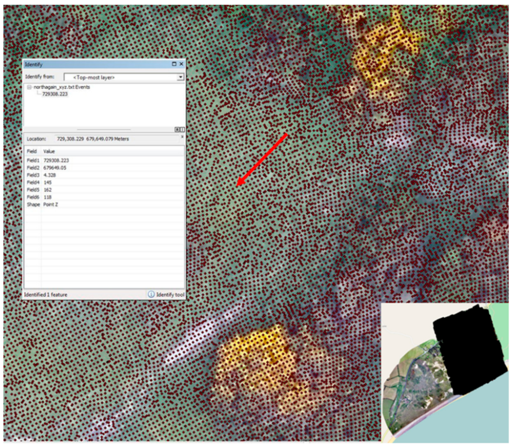
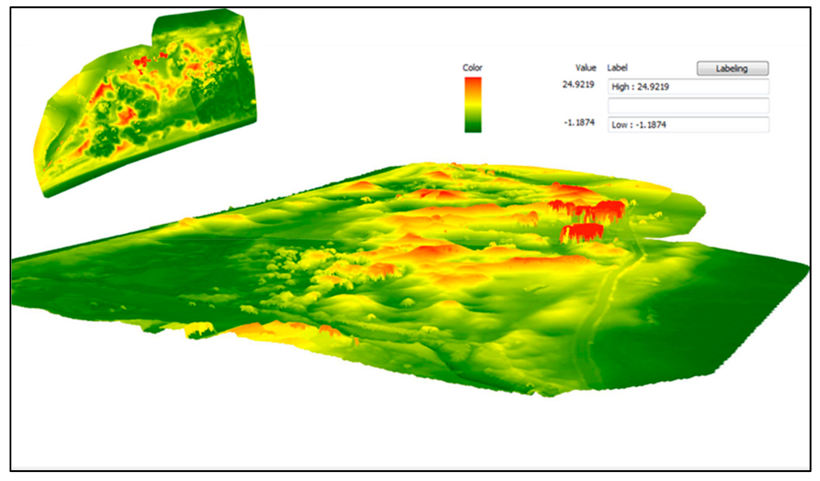
The imagery was processed using Pix4D software which generated a 3D point cloud (Figure 8), an orthomosaic model (Figure 9), a DSM from the RGB imagery (Figure 10) and a NDVI index map (Figure 11) which was generated from the multispectral imagery.
In addition, seven individual multispectral waveband orthomosaics (red, green, blue from normal RGB camera and red, green, red edge, near-infrared from multispectral sensor) of the site were created. These results were all referenced to the Irish Transverse Mercator (ITM) grid coordinate system. Ground sample distance (GSD) in a digital imagery of the ground from the air and is the distance between pixel centres measured on the ground. Outcomes from the RGB imagery had a GSD of 0.029 m and a georeferencing root mean square (RMS) error of 0.111 m.
Georeferencing of multispectral imagery by reference to the GCPs is not supported within the Pix4D software. Multispectral imagery is georeferenced by reference to the on-board autonomous GNSS data included in the imagery EXIF files. Six GCPs were identified in the outcome models and used as check points for outcome accuracy assessment. The multispectral imagery had a spatial resolution of 0.096 m and a georeferencing accuracy of 0.798 m.
5.2. Spectral Analysis
From the orthomosaic model generated from the captured imagery, eight dominant vegetation areas, including pasture, rusty willow, gorse, sharp rush, marram, common reed and mosses land, and another four significant contiguous land cover types were identified on the site, viz. road, beach, stream, sand and built area. Spectral patterns for these 12 types were analysed in the available seven wavebands, viz. green, red, near-infrared (NIR) and red edge from the multispectral sensor and red, green, blue wavebands extracted from RGB imagery. Figure 12 shows the spectral patterns of the twelve land cover types using these seven available wavebands.
As can be seen in Figure 12, “sand” and “stream” have significantly different responses under these seven available wavebands from the RGB camera and the multispectral sensor, which make them separable in the land feature classification. “Beach” has a distinctly separate response from other land cover types in the blue waveband extracted from the RGB camera and the red wavebands from the multispectral sensor, which means “beach” could be classified by considering the spectral pattern in only these two wavebands. Other land cover types have less separated responses in these available wavebands which make it more difficult to spectrally differentiate them. Thus, separable response value in available wavebands from the RGB camera and the multispectral sensor can only be used to identify “sand”, “stream” and “beach”; other land cover features are hard to be classified using response values in available wavebands.
Figure 12 also shows that vegetation land cover features have quite disparate spectral patterns in the RGB-derived bands but similar spectral patterns in the four wavebands of the multispectral sensors. The multispectral sensor-derived patterns all feature low responses at green and red wavebands and relatively higher responses at NIR and red edge wavebands. Non-vegetation land cover features do not follow this pattern and do not exhibit similar characteristic spectral patterns. Therefore, the characteristic spectral pattern of vegetation land features in the multispectral sensor-derived bands can be used to distinguish and separate vegetation and non-vegetation land features in the site.
In general, land cover features have characteristic spectral responses, in terms of both pattern and response value, which can be used as a basis for land cover features classification.
5.3. Classification Accuracy
In this study, to examine the efficiency of a multispectral sensor at vegetation mapping, accuracies of classifications were compared using different classification strategies (as shown in Table 4), including a combination of different multispectral wavebands and vegetation indices, calculated by multispectral wavebands. Classification accuracy was calculated by comparing the ground truth information and classified information in 245 samples through matrix analysis as seen in Table 5. Figure 13 shows the vegetation map of the site as the result of classification.
Through the matrix, the accuracies based on different classification strategies (in Table 4) were calculated (Figure 14). 3RGB means the classification layer is the combination of red, green and blue wavebands from the RGB camera, as seen in Table 4 (#1); 4MTB means the classification layer is the combination of green, red, red edge and near-infrared from multispectral sensor, as seen in Table 4 (#2); 7MTB means the classification layer is the combination of all available multispectral wavebands, as seen in Table 4 (#3); 8MTB_DSM, 8MTB_RG, 8MTB_RR, 8MTB_RB, 8MTB_NDVI, 8MTB_gNDVI, 8MTB_GRVI and 8MTB_NI were represented by #4–9 in Table 4, respectively.
The classification accuracy results (Figure 14) illustrate that multispectral sensor waveband data help to improve the accuracy as, for example, the classification accuracy based on 7MTB is higher than that based on 3RGB. Adding more wavebands from a multispectral sensor provides more reflectance information for classification and may help to improve the classification accuracy, such as 8MTB_RG (76%), 8MTB_RR (76%), 8MTB_RB (77%), 8MTB_NDVI (78%) and 8MTB_GRVI (77%) has higher accuracy than 7MTB (74%).
However, adding more reflectance information from the combination of wavebands did not always translate to an improvement in the classification accuracy. For example, 8MTB_DSM (71%) and 8MTB_gNDVI (72%) have lower accuracies than 7MTB (74%).
The classification accuracy of different classification strategies may also be influenced by image resolution. The multispectral sensor and RGB camera have different resolutions, being 1.2 MP and 16 MP, respectively. This may lead to the classification accuracy of 4MTB (60%), from the multispectral sensor data, being lower than 3RGB (69%) from the RGB camera data. Although a lower spatial resolution can have a smoothing effect that can, sometimes, lead to a higher classification accuracy.
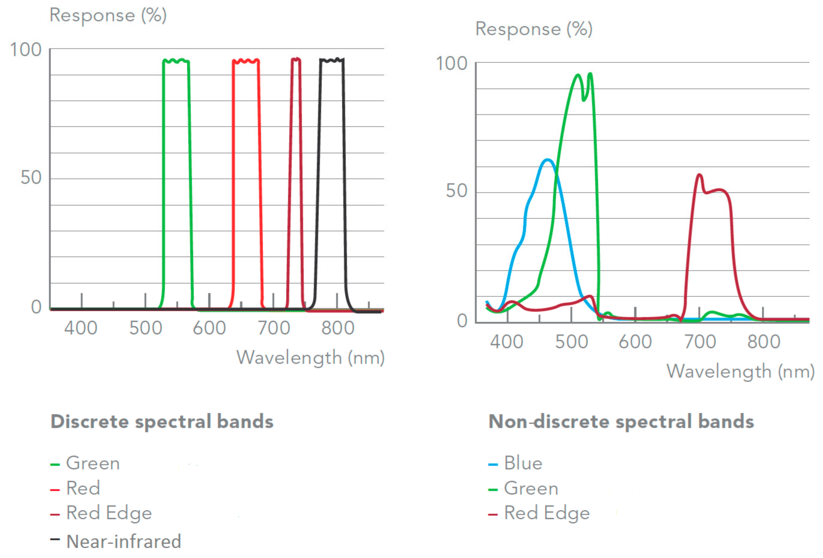
In addition, the RGB camera contains three non-discrete spectral bands, whereas the multispectral sensor has four discrete spectral bands. As seen in Figure 15, non-discrete spectral bands have a distinctly curved response and each band has considerable overlap in the wavelength range, whereas the discrete spectral bands of the multispectral sensor have an even response without overlap [41,42]. This should result in the multispectral wavebands providing more reliable reflectance patterns for land feature classification.
6. Conclusions
High-resolution vegetation and contiguous land cover mapping were successfully generated from imagery captured using a Sequoia multispectral sensor mounted on a UAS. The highest classification accuracy (78%) was achieved using eight spectral bands which included three wavebands from the RGB camera, four wavebands from the multispectral sensor and the NDVI index. Whereas using the three wavebands from the RGB camera and the four wavebands from the multispectral sensor, in combination, achieved a classification accuracy of 75%. Classification accuracy using only the four multispectral wavebands, was lower than the accuracy using the three wavebands of the RGB camera. Factors including image resolution, number of wavebands used, spectral separability and index type may contribute to the observed different classification accuracies using different classification strategies.
This research also highlighted an effective option for on-site surveying, significantly reducing the hazards and workload for the development of vegetation maps and DEMs of a study area. Using the multispectral sensor resulted in data captured from a wider range of wavebands than an RGB camera alone, with better resolution and accuracy than other conventional remote sensing technologies, enabling the generation of dense 3D point clouds, and orthomosaic models, DEMs and NDVI maps. In these outcomes, vegetation distribution and elevation changes over the Buckroney dune complex were represented clearly. The classification results also illustrated the high accuracy achieved for identifying different vegetation and contiguous land cover.
However, notwithstanding the many benefits and advantages of UAS and multispectral technology in vegetation mapping, the technology still has some challenges with respect to dune complex surveying. One issue is the permission, licensing, training required and restrictions to areas of UAS flight from the relevant aviation authority. As different countries have varying legislation controlling UAS use, it is recommended to be well-informed about the limitations on UAS use before the start of any UAS project. Although the use of a UAS platform can save much time at the on-site data collecting stage, a considerable amount of time is required for data processing. Furthermore, compared to other conventional survey methods, UAS is less robust as it is significantly impacted by environmental factors such as wind, precipitation and poor light conditions.
Author Contributions
Conceptualization, C.S. and E.M.; methodology, C.S. and E.M.; software, C.S.; validation, C.S. and E.M.; formal analysis, C.S.; resources, C.S.; data curation, C.S.; writing—original draft preparation, C.S.; writing—review and editing, E.M.; supervision, E.M. and A.G.
Funding
This work was funded by the Fiosraigh scholarship programme at the Technological University Dublin.
Acknowledgments
This work was funded by the Fiosraigh scholarship programme of the Technological University Dublin. The authors wish to acknowledge Eugene McGovern and Pengyu Chen for assistance in data collection in the field work.
Conflicts of Interest
The authors declare no conflicts of interest.
References
- Frosini, S.; Lardicci, C.; Balestri, E. Global Change and Response of Coastal Dune Plants to the Combined Effects of Increased Sand Accretion (Burial) and Nutrient Availability. PLoS ONE 2012, 7, e47561. [Google Scholar] [CrossRef] [PubMed]
- Fenu, G.; Cogoni, D.; Ferrara, C.; Pinna, M.S.; Bacchetta, G. Relationships between coastal sand dune properties and plant community distribution: The case of Is Arenas (Sardinia). Plant Biosyst. 2012, 146, 586–602. [Google Scholar] [CrossRef]
- McKenna, J.; O’Hagan, A.M.; Power, J.; Macleod, M.; Cooper, A. Coastal dune conservation on an Irish commonage: Community-based management or tragedy of the commons. Geogr. J. 2007, 173, 157–169. [Google Scholar] [CrossRef]
- Sabatier, F.; Anthony, E.J.; Hquette, A.; Suanez, S.; Musereau, J.; Ruz, M.H.; Regnauld, H. Morphodynamics of beach/dune systems: Examples from the coast of France. Géomorphologie 2009, 15, 3–22. [Google Scholar] [CrossRef]
- Woo, M.K.; Fang, G.X.; DiCenzo, P.D. The role of vegetation in the retardation of soil erosion. Catema 1997, 29, 145–159. [Google Scholar]
- Kuplich, T.M. Classifying regenerating forest stages in Amazonia using remotely sensed images and a neural network. For. Ecol. Manag. 2006, 234, 1–9. [Google Scholar] [CrossRef]
- Vaca, R.A.; Golicher, D.J.; Cayuela, L. Using climatically based random forests to downscale coarse-grained potential natural vegetation maps in tropical Mexico. Appl. Veg. Sci. 2011, 14, 388–401. [Google Scholar] [CrossRef]
- Accuracy Assessment: Cowpens National Battlefield Vegetation Map (A NatureServe Technical Report). Available online: https://irma.nps.gov/DataStore/DownloadFile/575467 (accessed on 26 March 2018).
- Yu, L.F.; Zhu, S.Q.; Ye, J.Z.; Wei, L.M.; Chen, Z.G. A study on evaluation of natural restoration for degraded karst forest. Sci. Silvae Sin. 2000, 36, 12–19. [Google Scholar]
- Song, C.H.; Schroeder, T.A.; Cohen, W.B. Predicting temperate conifer forest successional stage distributions with multitemporal Landsat Thematic Mapper imagery. Remote Sens. Environ. 2007, 106, 228–237. [Google Scholar] [CrossRef]
- Verbesselt, J.; Hyndman, R.; Newnham, G.; Culvenor, D. Detecting trend and seasonal changes in satellite image time series. Remote Sens. Environ. 2010, 114, 106–115. [Google Scholar] [CrossRef]
- Qi, X.K.; Wang, K.L.; Zhang, C.H. Effectiveness of ecological restoration projects in a karst region of southwest China assessed using vegetation succession mapping. Ecol. Eng. 2013, 54, 245–253. [Google Scholar] [CrossRef]
- Kozhoridze, G.; Orlovsky, N.; Orlovsky, L.; Blumberg, D.G.; Golan-Goldhirsh, A. Remote sensing models of structure-related biochemicals and pigments for classification of trees. Remote Sens. Environ. 2016, 186, 184–195. [Google Scholar] [CrossRef]
- Launeau, P.; Giraud, M.; Ba, A.; Moussaoui, S.; Robin, M.; Debaine, F.; Lague, D.; Le Menn, E. Full-Waveform LiDAR Pixel Analysis for Low-Growing Vegetation Mapping of Coastal Foredunes in Western France. Remote Sens. 2018, 10, 669. [Google Scholar] [CrossRef]
- Baltsavias, E.P. Airborne laser scanning: Existing systems and firms and other resources. ISPRS J. Photogramm. Remote Sens. 1999, 54, 164–198. [Google Scholar] [CrossRef]
- Highly Accurate Digital Terrain Models (DTM) or Digital Surface Models (DSM) (Ordnance Survey Ireland). Available online: https://www.osi.ie/wp-content/uploads/2015/05/Lidar_prod_overview.pdf (accessed on 20 February 2018).
- Anderson, K.; Gaston, K.J. Lightweight unmanned aerial vehicles will revolutionize spatial ecology. Front. Ecol. Environ. 2013, 11, 138–146. [Google Scholar] [CrossRef] [Green Version]
- Kaneko, K.; Nohara, S. Review of effective vegetation mapping using the UAV (Unmanned Aerial Vehicle) method. Int. J. Geogr. Inf. Sci. 2014, 6, 733–742. [Google Scholar] [CrossRef]
- Pajares, G. Overview and current status of remote sensing applications based on unmanned aerial vehicles (UAVs). Photogr. Eng. Remote Sens. 2015, 81, 281–329. [Google Scholar] [CrossRef]
- Weil, G.; Lensky, I.; Resheff, Y.; Levin, N. Optimizing the Timing of Unmanned Aerial Vehicle Image Acquisition for Applied Mapping of Woody Vegetation Species Using Feature Selection. Remote Sens. 2017, 9, 1–5. [Google Scholar] [CrossRef]
- Turner, I.L.; Harley, M.D.; Drummond, C.D. UAVs for coastal surveying. Coast. Eng. 2016, 114, 19–24. [Google Scholar] [CrossRef]
- Venturi, S.; Di Francesco, S.; Materazzi, F.; Manciola, P. Unmanned aerial vehicles and Geographical Information System integrated analysis of vegetation in Trasimeno Lake, Italy. Lakes Reserv. Res. Manag. 2016, 21, 5–19. [Google Scholar] [CrossRef]
- Bemis, S.P.; Micklethwaite, S.; Turner, D.; James, M.R.; Akciz, S.; Thiele, S.T.; Ali, H. Ground-based and UAV-based photogrammetry: A multi-scale, high-resolution mapping tool for structural geology and paleoseismology. J. Struct. Geol. 2014, 69, 163–178. [Google Scholar] [CrossRef]
- Tonkin, T.N.; Midgley, N.G. Ground-control networks for image based surface reconstruction: An investigation of optimum survey designs using UAV derived imagery and structure-from-motion photogrammetry. Remote Sens. 2016, 8, 786. [Google Scholar] [CrossRef]
- Uysal, M.; Toprak, A.S.; Polat, N. DEM generation with UAV Photogrammetry and accuracy analysis in Sahitler hill. Measurement 2015, 73, 539–543. [Google Scholar] [CrossRef]
- Ren, X.; Sun, M.; Zhang, X.; Liu, L. A Simplified Method for UAV Multispectral Images Mosaicking. Remote Sens. 2017, 9, 1–21. [Google Scholar] [CrossRef]
- Fernández-Guisuraga, J.M.; Sanz-Ablanedo, E.; Suárez-Seoane, S.; Calvo, L. Using Unmanned Aerial Vehicles in Postfire Vegetation Survey Campaigns through Large and Heterogeneous Areas: Opportunities and Challenges. Sensors 2018, 18, E586. [Google Scholar] [CrossRef] [PubMed]
- Gini, R.; Passoni, D.; Pinto, L.; Sona, G. Aerial images from an UAV system: 3d modeling and tree species classification in a park area. Int. Arch. Photogram. Remote Sens. Spat. Inf. Sci. 2012, 39, 361–366. [Google Scholar]
- Silleos, N.G.; Alexandridis, T.K.; Gitas, I.Z.; Perakis, K. Vegetation indices: Advances made in biomass estimation and vegetation monitoring in the last 30 years. Geocarto Int. 2006, 21, 21–28. [Google Scholar] [CrossRef]
- Helmer, E.H.; Brown, S.; Cohen, W.B. Mapping montane tropical forest successional stage and land use with multi-date Landsat imagery. Int. J. Remote Sens. 2000, 21, 2163–2183. [Google Scholar] [CrossRef]
- Huang, Q.H.; Cai, Y.L. Mapping karst rock in Southwest China. Mt. Res. Dev. 2009, 29, 14–20. [Google Scholar] [CrossRef]
- Liu, Q.J.; Takamura, T.; Takeuchi, N.; Shao, G. Mapping of boreal vegetation of a temperate mountain in China by multitemporal Landsat imagery. Int. J. Remote Sens. 2002, 23, 3385–3405. [Google Scholar] [CrossRef]
- Tokola, T.; Sarkeala, J.; Linden, M.V.D. Use of topographic correction in Landsat TM-based forest interpretation in Nepal. Int. J. Remote Sens. 2001, 22, 551–563. [Google Scholar] [CrossRef]
- Cuo, L.; Vogler, J.B.; Fox, J.M. Topographic normalization for improving vegetation classification in a mountainous watershed in Northern Thailand. Int. J. Remote Sens. 2010, 31, 3037–3050. [Google Scholar] [CrossRef]
- Elvidge, C.; Lyon, R. Influence of rock–soil spectral variation on the assessment of green biomass. Remote Sens. Environ. 1985, 17, 265–279. [Google Scholar] [CrossRef]
- Song, C.H.; Woodcock, C.E. Monitoring forest succession with multitemporal Landsat images: Factors of uncertainty. IEEE Trans. Geosci. Remote Sens. 2003, 41, 2557–2567. [Google Scholar] [CrossRef]
- Wilson, E.H.; Sader, S.A. Detection of forest harvest type using multiple dates of Landsat TM imagery. Remote Sens. Environ. 2002, 80, 385–396. [Google Scholar] [CrossRef]
- Franklin, S.E.; Lavigne, M.B.; Wulder, M.A.; McCaffrey, T.M. Large-area forest structure change detection: An example. Can. J. Remote Sens. 2002, 28, 588–592. [Google Scholar] [CrossRef]
- Gao, Y.N.; Zhang, W.C. A simple empirical topographic correction method for ETM plus imagery. Int. J. Remote Sens. 2009, 30, 2259–2275. [Google Scholar] [CrossRef]
- Site Synopsis: Buckroney-Brittas Dunes and Fen SAC (National Parks & Wildlife Service Site Documents). Available online: https://www.npws.ie/protected-sites/sac/000729 (accessed on 14 May 2018).
- Trimble RTX Frequently Asked Question. (Trimble Positioning Service Site). Available online: https://positioningservices.trimble.com/wp-content/uploads/2019/02/Trimble_RTX_Frequently_Asked_Questions.pdf (accessed on 23 July 2019).
- What Spectral Bands Does the Sequoia Camera Capture? (MicaSense Knowledge Base Site). Available online: https://support.micasense.com/hc/en-us/articles/217112037-What-spectral-bands-does-the-Sequoia-camera-captur (accessed on 12 May 2018).
Figure 1.
Morphology of the Brittas-Buckroney dune complex. Photo taken by the author.

Figure 2.
Photogrammetry-based 3D construction workflow of unmanned aerial systems (UAS) technology.
Figure 2.
Photogrammetry-based 3D construction workflow of unmanned aerial systems (UAS) technology.

Figure 3.
Study site (a) general location and (b) site details.

Figure 4.
Plant species at site (a) mosses land; (b) sharp rush (J. acutus); (c) European marram grass (A. arenaria); (d) gorse (U. europaeus); (e) common reed (P. australis); (f) rusty willow (S. cinerea subsp. oleifolia). Photos taken by the author.
Figure 4.
Plant species at site (a) mosses land; (b) sharp rush (J. acutus); (c) European marram grass (A. arenaria); (d) gorse (U. europaeus); (e) common reed (P. australis); (f) rusty willow (S. cinerea subsp. oleifolia). Photos taken by the author.


Figure 5.
Sequoia multispectral sensor mounted on a DJI Phantom 3 Pro UAS. Photo taken by the author.
Figure 5.
Sequoia multispectral sensor mounted on a DJI Phantom 3 Pro UAS. Photo taken by the author.

Figure 6.
Ground control points (GCPs) set on site for UAS surveying. Photo taken by the author.

Figure 7.
The balance card used for radiometric calibration.

Figure 8.
A sample of the 3D point cloud for the north section of study site.

Figure 9.
Orthomosaic model of the study site.

Figure 10.
Digital surface model (DSM) of the study site.

Figure 11.
NDVI map of the study site.

Figure 12.
Response of training samples in wavebands from (a) blue, green and red wavebands extracted from RGB camera; (b) green, red, NIR and red edge wavebands from multispectral sensor.
Figure 12.
Response of training samples in wavebands from (a) blue, green and red wavebands extracted from RGB camera; (b) green, red, NIR and red edge wavebands from multispectral sensor.

Figure 13.
Vegetation mapping of study site.

Figure 14.
Classification accuracy based on different strategies.

Figure 15.
Wavelength and response of discrete and non-discrete spectral bands.


Table 1.
Spectral indices calculated from four multispectral bands for vegetation mapping [20].
Table 1.
Spectral indices calculated from four multispectral bands for vegetation mapping [20].
| Spectral Indices | Formula | Explanation |
|---|---|---|
| Relative Green | The relative component of green, red and blue bands over the total sum of all camera bands. Less affected from scene illumination conditions than the original band value. | |
| Relative Red | ||
| Relative Blue | ||
| Normalized Differential Vegetation Index (NDVI) | Relationship between the near-infrared (NIR) and red bands indicates vegetation condition due to chlorophyll absorption within the red spectral range and high reflectance within the NIR range. | |
| gNDVI | Improvement of NDVI, accurate in assessing chlorophyll content. | |
| Green-Red Vegetation Index (GRVI) | Relationship between the green and red bands is an effective index for detecting phenophases. |
Table 2.
Parameters set for UAS flight mission.
| Flight Height | Overlapping along Line | Overlapping between Lines | Estimated Flight Time | Maximum Flight Speed |
|---|---|---|---|---|
| 80 m | 80% | 75% | 10 min | 10 m/s |
Table 3.
Parameters set for multispectral sensor mounted on UAS.
| Capture Mode | Interval Distance | Image Resolution | Bit Depth |
|---|---|---|---|
| Global Positioning System (GPS)-controlled | 15 m | 1.2 Mpx | 10-bit |
Table 4.
Band combination for different classification strategies.
| Classification Strategy | Band Combinations |
|---|---|
| Three wavebands from camera with red, green and blue wavebands (RGB camera) | 1. Red + Green + Blue |
| Four wavebands from multispectral sensor | 2. Green + Red + Red edge + NIR |
| Seven available multispectral wavebands | 3. Red + Green + Blue (from RGB) + Green + Red + Red edge + NIR (from multispectral) |
| Eight wavebands combinations | 4. Red + Green + Blue (from RGB) + Green + Red + Red edge + NIR (from multispectral) + Relative Green |
| 5. Red + Green + Blue (from RGB) + Green + Red + Red edge + NIR (from multispectral) + Relative Red | |
| 6. Red + Green + Blue (from RGB) + Green + Red + Red edge + NIR (from multispectral) + Relative Blue | |
| 7. Red + Green + Blue (from RGB) + Green + Red + Red edge + NIR (from multispectral) + NDVI | |
| 8. Red + Green + Blue (from RGB) + Green + Red + Red edge + NIR (from multispectral) + gNDVI | |
| 9. Red + Green + Blue (from RGB) + Green + Red + Red edge + NIR (from multispectral) + GRVI |
Table 5.
Sample matrix analysis for accuracy assessment.
| Column1 | Classified Data | ||||||||||||
|---|---|---|---|---|---|---|---|---|---|---|---|---|---|
| Road | Built Area | Sand | Stream | Beach | Pasture | Sharp Rush | Common Reed | Rusty Willow | Gorse | Mosses Land | Marram | ||
| Ground truth data | Road | 13 | 3 | 1 | 4 | 1 | |||||||
| B_A | 2 | 16 | 3 | ||||||||||
| Sand | 16 | 2 | 1 | 2 | |||||||||
| Str | 1 | 17 | 2 | 1 | |||||||||
| Beach | 1 | 14 | |||||||||||
| Past | 16 | ||||||||||||
| S_R | 14 | ||||||||||||
| C_R | 1 | 15 | 5 | 2 | 1 | ||||||||
| R_W | 1 | 8 | |||||||||||
| Gorse | 2 | 1 | 16 | 1 | |||||||||
| M_L | 3 | 1 | 1 | 17 | |||||||||
| Mar | 1 | 1 | 5 | 5 | 1 | 2 | 15 | ||||||
© 2019 by the authors. Licensee MDPI, Basel, Switzerland. This article is an open access article distributed under the terms and conditions of the Creative Commons Attribution (CC BY) license (http://creativecommons.org/licenses/by/4.0/).
Share and Cite
MDPI and ACS Style
Suo, C.; McGovern, E.; Gilmer, A. Coastal Dune Vegetation Mapping Using a Multispectral Sensor Mounted on an UAS. Remote Sens. 2019, 11, 1814. https://0-doi-org.brum.beds.ac.uk/10.3390/rs11151814
AMA Style
Suo C, McGovern E, Gilmer A. Coastal Dune Vegetation Mapping Using a Multispectral Sensor Mounted on an UAS. Remote Sensing. 2019; 11(15):1814. https://0-doi-org.brum.beds.ac.uk/10.3390/rs11151814
Chicago/Turabian StyleSuo, Chen, Eugene McGovern, and Alan Gilmer. 2019. "Coastal Dune Vegetation Mapping Using a Multispectral Sensor Mounted on an UAS" Remote Sensing 11, no. 15: 1814. https://0-doi-org.brum.beds.ac.uk/10.3390/rs11151814
Note that from the first issue of 2016, this journal uses article numbers instead of page numbers. See further details here.