Article

Tensor Discriminant Analysis via Compact Feature Representation for Hyperspectral Images Dimensionality Reduction

1
School of Information Engineering, Henan Institute of Science and Technology, Xinxiang 453003, China
2
Key Laboratory of Intelligent Perception and Image Understanding of Ministry of Education, Xi’an 710071, China
*
Author to whom correspondence should be addressed.
Remote Sens. 2019, 11(15), 1822; https://0-doi-org.brum.beds.ac.uk/10.3390/rs11151822
Submission received: 1 July 2019 / Revised: 26 July 2019 / Accepted: 29 July 2019 / Published: 4 August 2019
(This article belongs to the Special Issue Advanced Techniques for Spaceborne Hyperspectral Remote Sensing)

Abstract

:
Dimensionality reduction is of great importance which aims at reducing the spectral dimensionality while keeping the desirable intrinsic structure information of hyperspectral images. Tensor analysis which can retain both spatial and spectral information of hyperspectral images has caused more and more concern in the field of hyperspectral images processing. In general, a desirable low dimensionality feature representation should be discriminative and compact. To achieve this, a tensor discriminant analysis model via compact feature representation (TDA-CFR) was proposed in this paper. In TDA-CFR, the traditional linear discriminant analysis was extended to tensor space to make the resulting feature representation more informative and discriminative. Furthermore, TDA-CFR redefines the feature representation of each spectral band by employing the tensor low rank decomposition framework which leads to a more compact representation.

1. Introduction

Hyperspectral images can offer wealth ground objects information which make the precision analysis of different material come true. On the other hand, the high spectral dimensionality not only leads to high computational and storage costs but also degrade the processing performance especially when the training samples are scarce, which is known as “curse of dimensionality”. Dimensionality reduction (DR) is a critical preprocessing of hyperspectral images which aims at reducing the spectral dimensionality while keeping the desirable intrinsic structure information of hyperspectral images [1,2].
According to whether the labeled training samples are used or not, the existing dimensionality reduction methods can be categorized into three categories: unsupervised, supervised and semi-supervised. The labeled samples are needed in supervised methods which may lead to a more discriminative low dimensionality subspace, but the cost of labeling samples in hyperspectral images is extreme high which may limit the application of these methods in practice. The most widely used supervised dimensionality reduction is Linear Discriminant Analysis (LDA). The unsupervised methods obtain the low dimensionality representation by mining the structure characters of original dataset and need no label samples and Principal Components Analysis (PCA) is the most famous unsupervised criterion. To jointly consider the advantages of supervised and unsupervised methods, the semi-supervised criterion utilizes the label information from a few labeled samples and the structure information extracted from a large number of unlabeled samples [3,4].
From another perspective, the existing DR methods can also be classified into two types: feature extraction [5,6,7] and feature selection [8,9]. When feature selection is concerned, it refers to select feature subset which can retain the most original information of hyperspectral images according to some designed criteria. While feature extraction refers to project the original dataset into a low dimensionality with a designed project matrix.
A lot of dimensionality reduction methods have been proposed, but how to obtain a desirable lower dimensionality feature representation of original hyperspectral images remains a challenge. LDA is the most popular discriminant analysis criterion which aims at projecting the original high dimensionality dataset to a lower dimensionality subspace where the samples with the same labels are close to each other and the samples with different labels are apart from each other. With the advantages of enhance the discrimination of projected dataset, LDA has been widely used in subspace learning community [10,11,12,13]. In traditional LDA based methods, the original cube hyperspectral images have to be converted to matrix and the corresponding pixel samples is presented in vector form, the vectorization processing may destroy the intrinsic spatial region structure information.
To overcome the disadvantage of vectorization, a multilinear algebra framework, i.e., tensor analysis has been introduced to the community of hyperspectral images processing [14,15,16,17,18,19]. By presenting the original cube image as a 3-order tensor, tensor analysis can deal with the tensor samples directly. Furthermore, to jointly consider the advantages of discriminant analysis and tensor analysis, the traditional LDA model has been extended to tensor space via different criteria. Yan et al. [20] proposed a multilinear discriminant analysis (MDA) model which treated the original images as a two or three order tensor and achieved supervised dimensionality reduction. Tao et al. [21] extended the differential scatter discriminant criterion (DSDC) model to tensor space and constructed the general tensor discriminant analysis (GTDA) framework. Nie et al. proposed a local within class scatter matrix criterion which overcome the drawback of Gaussian hypothesis in LDA [22]. Zhong et al. proposed an integrated spatial-spectral feature extract method for original hyperspectral images under the tensor analysis framework which can characterize the intrinsic formation of the original hyperspectral images more efficiently [23]. By constructing the same class and different class patch with tensor samples, Zhang et al. proposed the discriminative analysis by maximizing the distances of different class while minimizing the distances of different class [19].
It can be observed from the analysis above that, extracting the intrinsic spatial-spectral information of the original hyperspectral images and enhancing the discriminant ability are two critical issues in hyperspectral images dimensionality reduction. In vector samples based discriminant analysis methods, the spatial neighborhood information of hyperspectral images may be destroyed during the process of vectorization which may degrade the performance of dimensionality reduction. In addition, some tensor based discriminant analysis methods extend the discriminant analysis model into tensor space to make the processed dataset more discriminantive, but these methods are directly implemented on the raw spectral bands which may degrade the dimensionality reduction performance due to the redundant, scattered and chaotic spectral information distribution.
In general, the compact feature representation is more informative and representative [24]. When hyperspectral images are concerned, the wealthy spectral information makes the analysis of land covers more efficient. It is noted that, the original information of hyperspectral images is distributed in all the spectral bands randomly, and the information offered by different bands may be scattered, or even chaotic and conflicting. All these may degrade the representative ability of original spectral bands. To alleviate the conflict of different bands and derive a compact feature representation, a low rank tensor decomposition based compact feature representation method (TDA-CFR) is proposed. In TDA-CFR, hyperspectral image is treated as a 3-order tensor dataset, and a novel tensor decomposition criterion is proposed to eliminate the spectral redundant information and make the resulting feature representation more compact and informative. The flowchart of the proposed TDA-CFR is shown in Figure 1.
The main contributions of this paper can be concluded from three points: (1) by employing the fixed spatial window criterion, the proposed TDA-CFR constructs the training samples in 3-order tensor form which can well preserve the spatial neighborhood information and lead to a more effective representation of the hyperspectral image. (2) by employing tensor low rank criterion, the proposed method obtains a more compact feature representation which can eliminate the chaotic and conflicting information offered by different bands. (3) by integrating the compact feature representation into the tensor discriminant analysis framework, the proposed method obtains a compact and discriminative feature representation.
The rest of this paper is arranged as follows. Some related works are introduced in Section 2. TDA-CFR is described detailed in Section 3. In Section 4, experiments are conducted to evaluate the performance of TDA-CFR. Some important issues of the proposed method are discussed in Section 4 and Section 5 shows the conclusion of this paper.

2. Related Work

2.1. Linear Discriminant Analysis

LDA [25] aims at finding a projection direction which can ensure the samples with the same labels are as close as possible in the low dimensionality subspace, while samples belonging to different classes are far from each other. Suppose there are C classes of all samples and x i j denotes the samples j belonging to class i, n i is the training samples number of class i, m i is the mean values of the samples belonging to class i and m is the mean value of all samples. Then the within class scatter matrix can be defined as [21]
S w = 1 n i = 1 C j = 1 n i ( x i j - m i ) ( x i j - m i ) T
similarly, the between class scatter matrix can be defined as
S b = 1 n i = 1 C n i ( m i - m ) ( m i - m ) T
With the difference scatter discriminant criterion, the objective function of LDA can be represented as
arg max U t r { U ( S b - ζ S w ) U T }
where ζ is a tuning parameter and U is the optimal projection matrix.

2.2. Tensor Analysis

In this section, some basic tensor operations are presented. For an N-order tensor X R I 1 × I 2 × × I N , the related tensor operations are elaborated as follows.
n-mode flattening matrix: By fixing all the indices of X except i n , we can obtain the n-mode vectors of X . n-mode flattening matrix is constructed by taking all the n-mode vectors in columns which can be represented as
X n R I n × ( I 1 × I 2 × I n - 1 × I n + 1 × × I N )
n-mode product: Given a matrix U R J × I n , the n-mode product can be denoted as Y = X × n U , where the symbols “ X × n U ” means the tensor X products matrix U along mode n and Y R I 1 × × J × × I N with elements Y i 1 i 2 i n - 1 j i n + 1 i N = i n = 1 I n x i 1 i 2 i n - 1 i n i n + 1 i N u j i n . In addition, the n-mode product can be denoted in a matrix form
Y = X × n U Y n = U X n
Tucker decomposition: Given the factor matrices U n R I n × R n ( 1 n N ) , Tucker decomposition can be formulated as
Y = X × 1 U 1 × 2 U 2 × × N U N = r 1 = 1 R 1 r 2 = 1 R 2 r N = 1 R N x r 1 r 2 r N u 1 r 1 u 2 r 2 u N r N
where “∘” is the outer product of the vectors.
Tensor Frobenius norm: The tensor Frobenius norm is calculated by
X F = i 1 = 1 I 1 i 2 = 1 I 2 i N = 1 I N x i 1 i 2 i N 2

3. Tensor Discriminant Analysis via Compact Feature Representation

3.1. Tensor Discriminant Analysis

In this section, the traditional LDA is extended to tensor discriminant analysis (TDA). Suppose p tensor samples, i.e., X 1 , X 2 , , X p R I 1 × I 2 × × I N , belong to C classes, n i is the samples number of class i, i.e., p = i = 1 c n i . Let X i j represent the j-th sample of class i, the mean tensor of class i can be denoted as M i = 1 n i j = 1 n i X i j and the mean tensor of all samples can be denoted as M = 1 p i = 1 c j = 1 n i X i j = 1 p i = 1 c n i M i .
Similar to the discussion above, TDA aims at finding a series of factor matrices U 1 , U 2 , , U N , U n R I n × I n ( n = 1 , 2 , N ) to project the original tensor dataset to a low dimensionality subspace,
Y i j = X i j k = 1 N × k U k T R I 1 × I 2 × × I N
where Y i j is the projected data of X i j .
The projected mean tensor of class i in the low dimensionality subspace can be represented as
M ˜ i = 1 n i j = 1 n i Y i j = 1 n i j = 1 n i ( X i j k = 1 N × k U k T ) = M i k = 1 N × k U k T
Similarly, the projected mean tensor of all samples in the low dimensionality subspace can be denoted as
M ˜ = M k = 1 N × k U k T
It is noted that, the solution of k factor matrices in Equations (9) and (10) are high order optimization problems which cannot be solved simultaneously. An iteration scheme is adopted to calculate the optimal factor matrices by solving one factor matrix at a time while with the remaining fixed [26]. To apply this iteration scheme, the tensor samples are flattened along mode n and the between class scatter matrix can be denoted as
B n = i = 1 c n i [ ( M i k = 1 N × k U k T ) ( n ) - ( M k = 1 N × k U k T ) ( n ) ] [ ( M i k = 1 N × k U k T ) ( n ) - ( M k = 1 N × k U k T ) ( n ) ] T = i = 1 c n i [ ( M i - M ) k = 1 N × k U k T ] ( n ) [ ( M i - M ) k = 1 N × k U k T ] ( n ) T = U n T { i = 1 c n i [ ( M i - M ) k = 1 , k n N × k U k T ] ( n ) [ ( M i - M ) k = 1 , k n N × k U k T ] ( n ) T } U n = U n T B n n ¯ U n
where B n n ¯ = i = 1 c n i [ ( M i - M ) k = 1 , k n N × k U k T ] ( n ) [ ( M i - M ) k = 1 , k n N × k U k T ] ( n ) T is the projected between class scatter matrix except mode n.
Similarly, the n mode within class scatter matrix can be defined as
W n = i = 1 c j = 1 n i [ ( X i j k = 1 N × k U k T ) ( n ) - ( M i k = 1 N × k U k T ) ( n ) ] [ ( X i j k = 1 N × k U k T ) ( n ) - ( M i k = 1 N × k U k T ) ( n ) ] T = i = 1 c n i [ ( X i j - M i ) k = 1 N × k U k T ] ( n ) [ ( X i j - M i ) k = 1 N × k U k T ] ( n ) T = U n T { i = 1 c j = 1 n i [ ( X i j - M i ) k = 1 , k n N × k U k T ] ( n ) [ ( X i j - M i ) k = 1 , k n N × k U k T ] ( n ) T } U n = U n T W n n ¯ U n
where W n n ¯ = i = 1 c j = 1 n i [ ( X i j - M i ) k = 1 , k n N × k U k T ] ( n ) [ ( X i j - M i ) k = 1 , k n N × k U k T ] ( n ) T is the projected within class scatter matrix along all modes except mode n.
To measure the distance of tensor samples in the low dimensionality subspace, the tensor Frobenius norm is chosen to calculate the distance of tensor samples. According the tensor operations, maximize the tensor Frobenius norm of the projected mean tensor can be reformulated as Equation (13)
arg max U n i = 1 c n i ( M i - M ) k = 1 N × k U k T F 2 = arg max U n t r { U n T W n n ¯ U n }
Similarly, minimize the tensor Frobenius norm of the projected mean tensor is equal to minimize the trace of mode n within class scatter matrix, which can be denoted as Equation (14)
arg min U n i = 1 c j = 1 n i ( X i j - M i ) k = 1 N × k U k T F 2 = arg min U n t r { U n T B n n ¯ U n }
By adopting the difference scatter discriminant criterion [21,27], the objective function of TLDA can be reformulated as Equation (15).
F ( U n ) = arg max U n t r { U n T B n n ¯ U n } - ξ t r { U n T W n n ¯ U n } s . t . U n U n T = I
where ξ is the tuning parameter.
Finally, the optimal factor matrix U n can be solved by Equation (16).
U n = arg max U n U n T = I t r { U n T ( B n n ¯ - ξ W n n ¯ ) U n }
The projected data of sample X i , j in low dimensionality subspace can be calculated by Equation (17).
Y i , j = X i , j × 1 U 1 × 2 U 2 × × N U N
The detailed steps of TDA are illustrated in Algorithm 1.
Algorithm 1: Tensor discriminant analysis
INPUT: Original cube hyperspectral image X R I 1 × I 2 × I 3 and the corresponding labels, the dimensionality of projection space I 1 × I 2 × I 3 , spatial size of tensor training samples B 1 and B 2 , the training samples number of each class n i , parameter ξ , maximum iteration number T max and iteration error tolerance ε .
Construct n i tensor training samples for each class with spatial size B 1 × B 2
Initialize U n 0 = I I n × I n .
For t = 1 , 2 , T max
      For n = 1 , 2 , , N do
           compute B n n ¯ by Equation (11).
           compute W n n ¯ by Equation (12).
           compute factor matrix U n by Equation (16).
      end
      check e r r o r ( t ) = n = 1 N U n t ( U n t - 1 ) T F ε
end
OUTPUT: The optimal factor matrices U n , n = 1 , 2 , 3 .

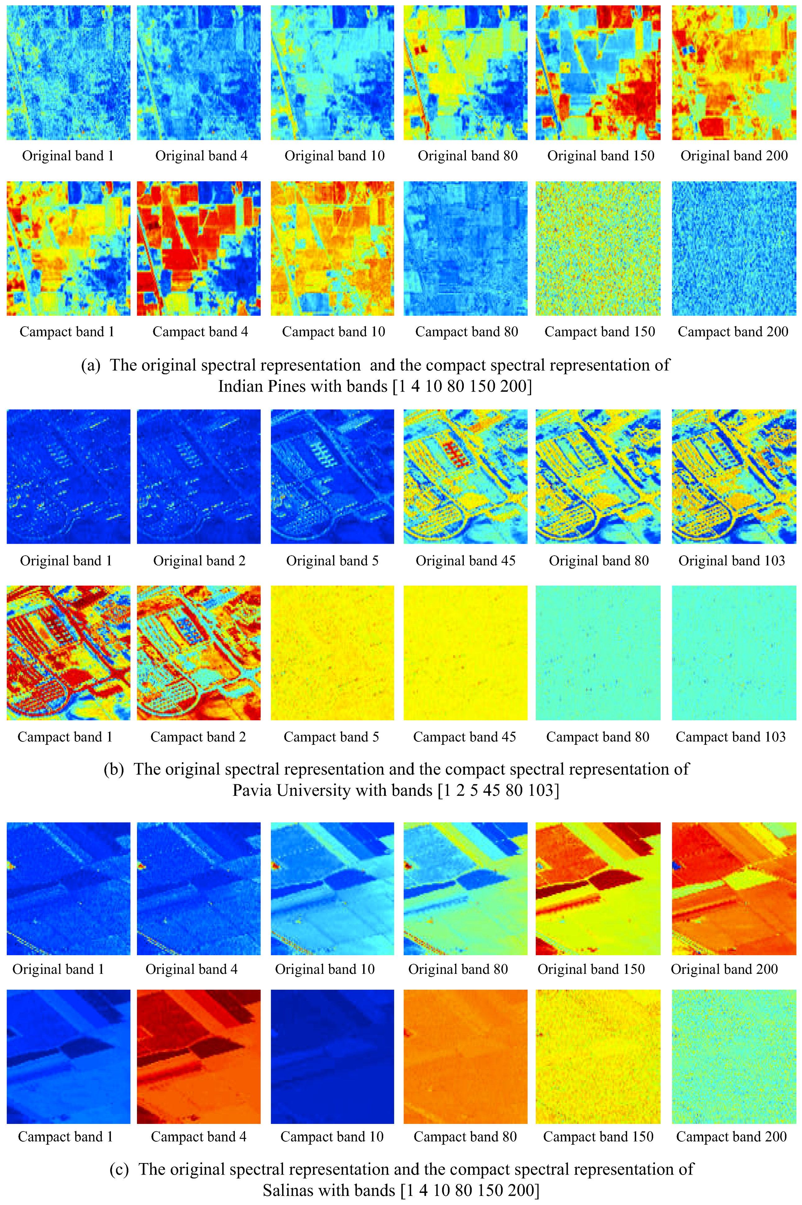
3.2. Compact Feature Representation of Hyperspectral Images

The large spectral bands number of hyperspectral images bring rich spectral information, but when the ability of representation is concerned, the original spectral bands may not be the ideal representation.There are at least two drawbacks of the original spectral bands: (1) there are redundancy information among different spectral bands, especially between the neighboring bands which may lead to the high computational and storage cost. (2) the intrinsic spectral feature of original hyperspectral images is randomly distributed in all the spectral bands, compared with the compact feature distribution, it is difficult to extract the disperse information from all the spectral bands. These two drawbacks may result in a chaos and even conflicting spectral representation which will degrade the representative of the original spectral bands. To overcome these drawbacks, a novel tensor analysis based compact feature representation method of hyperspectral images is proposed.
The original cube hyperspectral image can be directly presented as a 3 order tenser dataset, i.e., two spatial dimensions and one spectral dimension. Suppose a hyperspectral image X R I 1 × I 2 × I 3 , where I 1 and I 2 are the spatial dimensions and I 3 is the spectral dimension. The low rank tensor decomposition aims at finding a approximate tensor X ˜ R I 1 × I 2 × I 3 , which satisfies the Equation (18)
f ( X ˜ ) = argmin X - X ˜ F 2
where r a n k 1 ( X ˜ ) = r 1 , r a n k 2 ( X ˜ ) = r 2 , r a n k 3 ( X ˜ ) = r 3 is the given rank along each mode of X ˜ . It have been proved that, Equation (18) can be converted to Equation (19),
m a x U 1 , U 2 , U 3 X ˜ × 1 U 1 × 2 U 2 × 3 U 3 F 2
where U n , n = 1 , 2 , 3 is constructed by the first r n eigenvectors of R n R n T and R n is the n - mode flattening matrix of X ˜ [28]. The solution of Equation (19)can be represented as
X ˜ = X × 1 P 1 × 2 P 2 × 3 P 3
where P n = U n U n T , n = 1 , 2 , 3 .
The purpose of compact representation is to make the randomly distributed in all the spectral bands more concentrated. By extending the PCA to tensor space, the eigenvectors corresponding to the larger eigenvalues of R ˜ n R ˜ n T retains more intrinsic information of mode n.
Inspired by the analysis above, it can be concluded that, the concentration of spectral bands can be achieved by concentrating the eigenvalues corresponding to the covariance matrix R ˜ 3 R ˜ 3 T along spectral mode, so we resort the eigenvalues and represent the new eigenvalues array as δ . It is noted that, the spatial region neighborhood information of hyperspectral images must be kept, so the compact representation is only considered in spectral domain. Here, the rank along each mode is set to be equal to the original size of hyperspectral image, i.e., r 1 = I 1 , r 2 = I 2 , r 3 = I 3 . The compact representation of X ˜ can be calculated by Equation (21).
X c o m p a c t = X × 1 P 1 × 2 P 2 × 3 Λ - 1 / 2 U 3 T
where Λ is the diagonal matrix corresponding to δ .
To illustrate the effect of compact spectral feature representation, some selected raw bands and compact representation bands of three real hyperspectral images are shown in Figure 2. Figure 2a shows the raw and compact representation of Indian Pines dataset with the bands of [1 4 10 80 150 200], Figure 2b shows the raw and compact representation of Pavia University dataset with the bands of [1 2 5 45 80 103] and Figure 2c shows the raw and compact representation of Salinas dataset with the bands of [1 4 10 80 150 200]. It can be seen from Figure 2 that, for the raw representation, the spectral information is randomly distributed in all spectral bands which make it difficult to extract the intrinsic information of the hyperspectral images, while for the compact representation, the spectral information is mainly preserved in the first spectral bands and the latter bands contain little useful information.

3.3. Dimensionality Reduction of Hyperspectral Images by TDA-CFR

In general, a ideal feature representation of hyperspectral image should be compact and discriminative. To achieve this, a hyperspectral images dimensionality reduction model called tensor discriminant analysis via compact feature representation (TDA-CFR) is constructed by integrating the TDA and the compact representation. There are mainly three steps of the proposed model, i.e., compact spectral feature representation, tensor samples construction and dimensionality reduction.
For compact spectral feature representation, by setting the rank along each mode equal to the original size of the hyperspectral image, the compact spectral feature representation can be calculated by Equation (21).
To fully preserve the spatial region neighborhood information of the hyperspectral images, tensor samples are constructed for each pixels by a fixed spatial window B 1 × B 2 . For the compact representation X c o m p a c t R I 1 × I 2 × I 3 , the tensor samples dataset, which is called sub-tensor dataset can be represented as X c o m p a c t s u b R B 1 × B 2 × I 3 × ( I 1 × I 2 ) , where B 1 , B 2 is the spatial size of tensor samples, I 3 is the spectral dimensionality and I 1 × I 2 is the number of tensor samples.
In the framework of Tucker decomposition, the dimensionality reduction of tensor samples can be achieved by Equation (22),
Y i = X c o m p a c t s u b ( i ) × 1 U 1 × 2 U 2 × 3 U 3
where X c o m p a c t s u b ( i ) is the i-th tensor sample and Y i is the corresponding low dimensionality projection. The critical issue of Equation (22) is the factor matrices U n which can be calculated by Equation (16). In Equation (16), we select the first I n eigenvectors corresponding to ( B n n ¯ - ξ W n n ¯ ) along mode n and the factor matrices U n can be denoted as U n R I n × I n , I n > I n , n = 1 , 2 , 3 , where I n is the original size along mode n and I n is the reduction dimensionality along mode n. It is noted that, to keep the spatial dimensionality of hyperspectral image unchanged and reduce the spectral dimensionality, the spatial factor matrices U 1 , U 2 are constructed by the largest eigenvector along mode 1 and mode 2, while the factor matrix U 3 is constructed by the first I n eigenvector along mode 3. After rearranging the projected tensor samples Y i , the dimensionality reduction dataset Y R I 1 × I 2 × I 3 is obtained.
The detailed steps of TDA-CFR are shown in Algorithm 2.
Different form the existing tensor based discriminant analysis methods which are directly applied in the raw spectral bands of hyperspectral images, the proposed TDA-CFR integrates the tensor discriminant analysis and compact feature representation in one framework which can eliminate the chaotic and conflicting information of the raw spectral bands and lead to a more discriminative and informative feature representation. On the other hand, the tensor sample volume of TDA-CFR is larger than that of vector base methods due to the tensor samples criterion is employed in the proposed method which may result in a longer running time.
Algorithm 2: The Proposed TDA-CFR
INPUT: Original cube hyperspectral image X R I 1 × I 2 × I 3 , the spatial size of sub-tensor samples B 1 and B 2 , the training samples number of each class n i , parameter ξ , maximum iteration number T max and iteration error tolerance ε .
 Calculate the compact representation of hyperspectral image X c o m p a c t R I 1 × I 2 × I 3 by Equation (21).
 Construct n i tensor training samples for each class with spatial size B 1 × B 2
 Calculate the factor matrices U n , n = 1 , 2 , 3 by Algorithm 1.
 Calculate the low dimensionality projection of all tensor samples by Equation (22).
 Rearrange the projected dataset Y i .
OUTPUT: The dimensionality reduction dataset Y

4. Experimental Results and Analysis

The performance of TDA-CFR, i.e., the classification accuracy, the sensitivity with different number of spectral bands and the computation efficiency are presented in this section.

4.1. Experimental Setup

(1) Hyperspectral dataset
Three real hyperspectral images, namely Indian Pine, Pavia University and Salinas are selected as the experimental datasets in the following experiments [29]. The pseudo-color and ground truth maps of these three hyperspectral images are shown in Figure 3a,b, Figure 4a,b and Figure 5a,b respectively.
Indian Pines: there are 16 different land covers in this scene. The spatial size of Indian Pine is 145 × 145 . After removing the noisy bands, 200 bands are considered in spectral domain. Pavia University: The land covers in Pavia University are classified into 9 classes. The spatial size of this image is 610 × 340 and the number of spectral bands is 103. Salinas: this scene contains 16 different land covers. After removing 20 noisy bands, the cube size of this image is 512 × 217 × 204 .
(2) Comparison methods
The proposed TDA-CFR is a tensor discriminative analysis based dimensionality reduction method, some related methods, including Linear discriminant analysis (LDA), sparse and low rank graph for discriminant analysis (SLGDA) [30] which employs the sparse and low rank constraints to achieve dimensionality under the graph embedding framework, low rank tensor approximation (LRTA) [31] in which the tensor low rank decomposition criterion is directly implemented on the raw hyperspectral images, group tensor based low rank decomposition (GTLR) [32] in which the tensor samples of hyperspectral images are firstly grouped into some clusters and then the tensor low rank decomposition is implemented on the obtained clusters, tensor discriminant analysis without compact representation (TDA) is also chosen as the comparison method to evaluate the effect of compact feature representation, tensor sparse and low rank graph based discriminant analysis (TSLGDA) [33] which is a tensor graph method with sparse and low rank constraints and the raw spectral feature (Original) is chosen as the benchmark.
Two popular classifiers, i.e., the Support Vector Machine (SVM) and Nearest Neighborhood (1NN) and chosen as the classifiers. The Gaussian kernel function is employed in SVM and the parameters in SVM are obtained by the 5-flod cross validation. 10% training samples are randomly selected to train the classifiers and the remaining are used as testing samples. To reduce the effect of randomness, all experiments are repeated 100 times and the mean values and variance are reported.
Let N be the number of all samples, C be the number of all classes, N i be the samples number of class i and n i be the number of correctly classified samples of class i, the corresponding evaluation indexes can be defined as follows.
OA evaluates the percentage of correctly classified samples in the total samples which is defined by Equation (23).
O A = i = 1 C n i i = 1 C N i
AA measures the mean values of the correctly classified percentages of all classes which is denoted by Equation (24).
A A = 1 C i = 1 C n i N i
CA is the percentage of correctly classified samples for individual class which is defined by Equation (25).
C A i = n i N i
Kappa coefficient is a multivariate statistical method for evaluating classification accuracy which can take into account the uncertainty of classification results and reflect the error of classification more accurately. Suppose the confusion matrix M is denoted by Equation (26).
M = m 11 m 1 C m C 1 m C C
where m i j is the number of pixels which belong to class i and be classified to class j. Then, the Kappa can be calculated by Equation (27)
K a p p a = p o - p e 1 - p e
where p o = 1 N i = 1 C m i i , p e = 1 N 2 i = 1 C m i * m * i and m i * = j = 1 C m i j , m * i = j = 1 C m j i .
Kappa coefficient is between 0 and 1, and the higher Kappa coefficient means the better consistency of classification results.

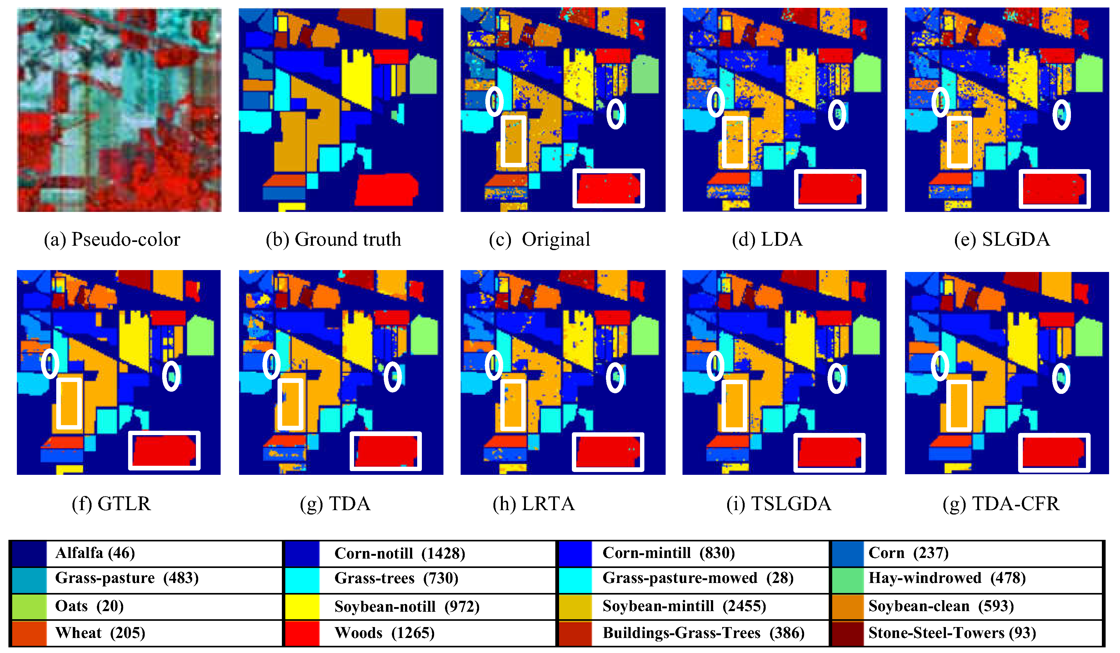
4.2. Classification Results

The separability of hyperspectral dataset after dimensionality reduction is an important index for dimensionality reduction. Classification experiments are employed to evaluate the separability of the dimensionality reduced hyperspectral dataset. The classification results (including OA, AA, Kappa coefficients and Class-special Accuracy) are listed in Table 1, Table 2 and Table 3, the classification maps are shown in Figure 3, Figure 4 and Figure 5.
Indian Pines is a relatively complicated scene, there are small sample classes (class 7 and 9, marked by) as well as the classes with good consistency (such as class 11 and 14, marked by white rectangle). TDA-CFR can obtain the best performance in terms of OA, AA and Kappa. Specifically, for the small samples classes, TDA-CFR achieves about 94% and 81% classification accuracy of class 7 and class 9. For the classes with large samples and good consistency, such as classes 11 and 14, TDA-CFR achieves about 98% and 99% classification accuracy of these two classes. The desirable classification performance reveals the good performance of TDA-CFR in dimensionality reduction. GTLR achieves the best classification performance of classes 7, but the classification performance greatly depends on the spatial size of tensor samples, the performance will degrades seriously if the spatial size is inappropriate.
For Pavia University, it can be concluded from Table 2 and Figure 4 that, for good spatial consistency classes (such as class 6, marked by white rectangle), the tensor based methods have evident advantages over vector based methods, which further reveals the superiority of tensor analysis in hyperspectral images processing. In addition, the proposed method also achieves desirable performance on the zonal and dotted classes (such as class 8, marked by white oval).
The ground objects in Salinas have relatively large samples number and good spatial consistency which leads to a good classification performance for all the comparing methods. It is noted that, by employing the tensor discriminative analysis and compact spectral feature representation, the proposed method achieves desirable classification performance of class 8 and 15 (marked by white oval) which are easy to confuse. In addition, the proposed TDA-CFR achieves almost 100% classification accuracy of classes 2, 3, 6, 9 and 12 with SVM classifier, which further demonstrates the excellent performance of the TDA-CFR at extracting the discriminative and compact intrinsic information of the hyperspectral images.

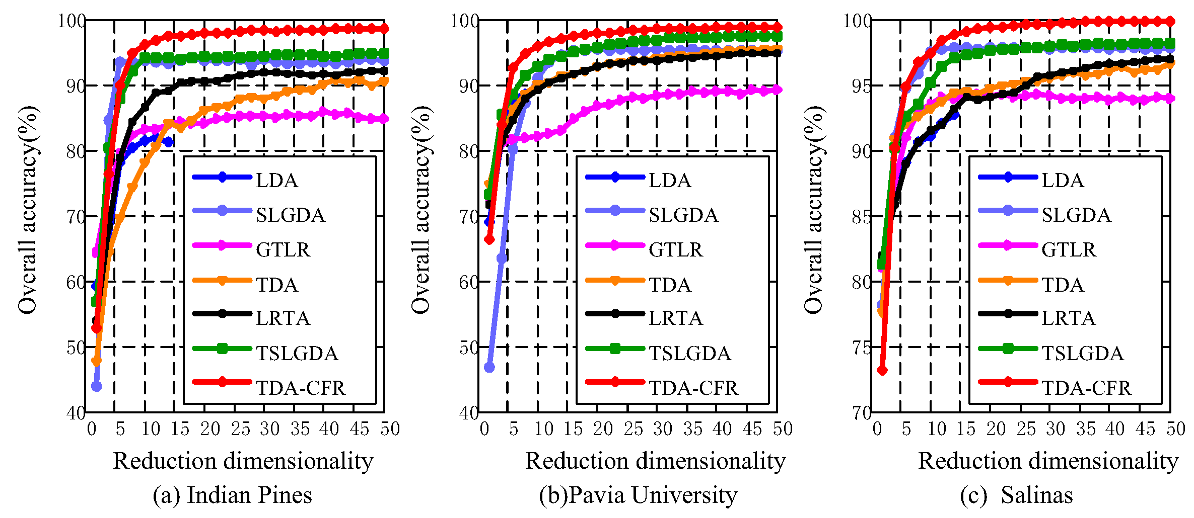
4.3. The Effect of Reduced Dimensionality

The classification accuracy with different spectral dimensionality is an important evaluation index of dimensionality reduction methods and this issue of TDA-CFR is analyzed experimentally in this section. The dimensionality range is set as (2–50) and the step size is 2. The results are shown in Figure 6 which illustrate that, for all comparison methods, the OA increases with the increase of dimensionality and then goes stabilized. In addition, TDA-CFR achieves the optimal classification performance when the dimensionality is larger than 20, which further reveals the good performance of TDA-CFR in hyperspectral images dimensionality reduction. According the experimental results, we set the reduced dimensionality as 30 in all these experiments.

4.4. Analysis of Computation Efficiency

The computation efficiency is analyzed in term of running time with Matlab R2014a on a PC with Intel Core i5-5490 CPU and 8G RAM. The results are listed in Table 4.
It can be observed from Table 4 that, for vector based methods, i.e., LDA, SLGDA, and ORIGINAL, the corresponding running time are shorter than that of tensor based methods, such as GTLR, TDA, LRTA, TSLGDA and TDA-CFR. More specifically, GTLR and LRTA cost the much shorter running time than the other tensor based methods, this is because the best rank values along each mode in these two methods are given directly and this avoids the complicated operation of rank estimation. Because the optimal factor matrices in TSLGDA are calculated by the iteration criterion which is time consuming, TSLGDA needs almost the longest running time. The running time of TDA and TDA-CFR are almost the same, this reveals most of the running time is consumed in the step of discriminant analysis.

5. Discussion

There are some parameters of the proposed TDA-CFT, such as the spatial size of tensor samples, the number of training samples and the tuning parameter. In this section, these parameters are discussed to evaluate the method more comprehensively.

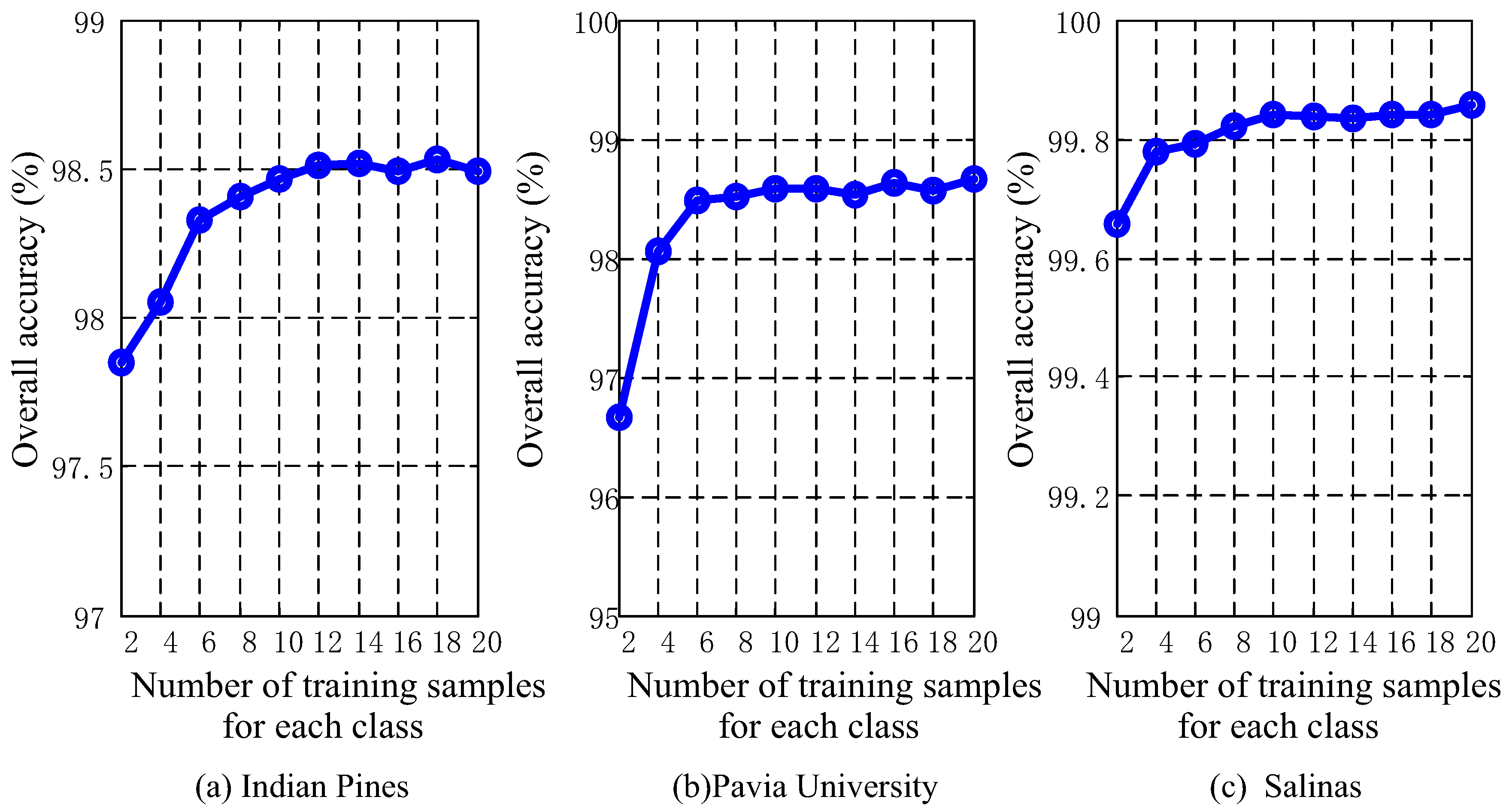
5.1. Discussion of the Number of Training Samples

Training samples number is an important issue for the proposed TDA-CFT. In this section, a classification experiment with SVM classifier with the training samples number varying from 2 to 20 and the results are shown in Figure 7. Generally speaking, the classification results increase with the increase of training samples number and then tend to be stable. It can be observed from Figure 7 that, the training samples number has slight effect on the OA and the proposed TDA-CFR can achieve desirable performance even there are only a few training samples number, this may be because one tensor samples usually contains many pixel samples, so there will still be a number of pixel samples which can offer rich intrinsic information of the hyperspectral images even only a few tensor samples are selected. This character will make the proposed TDA-CFT more practical when the labeled samples are scarce. The number of training samples for each class is set as 5 in all the experiments.

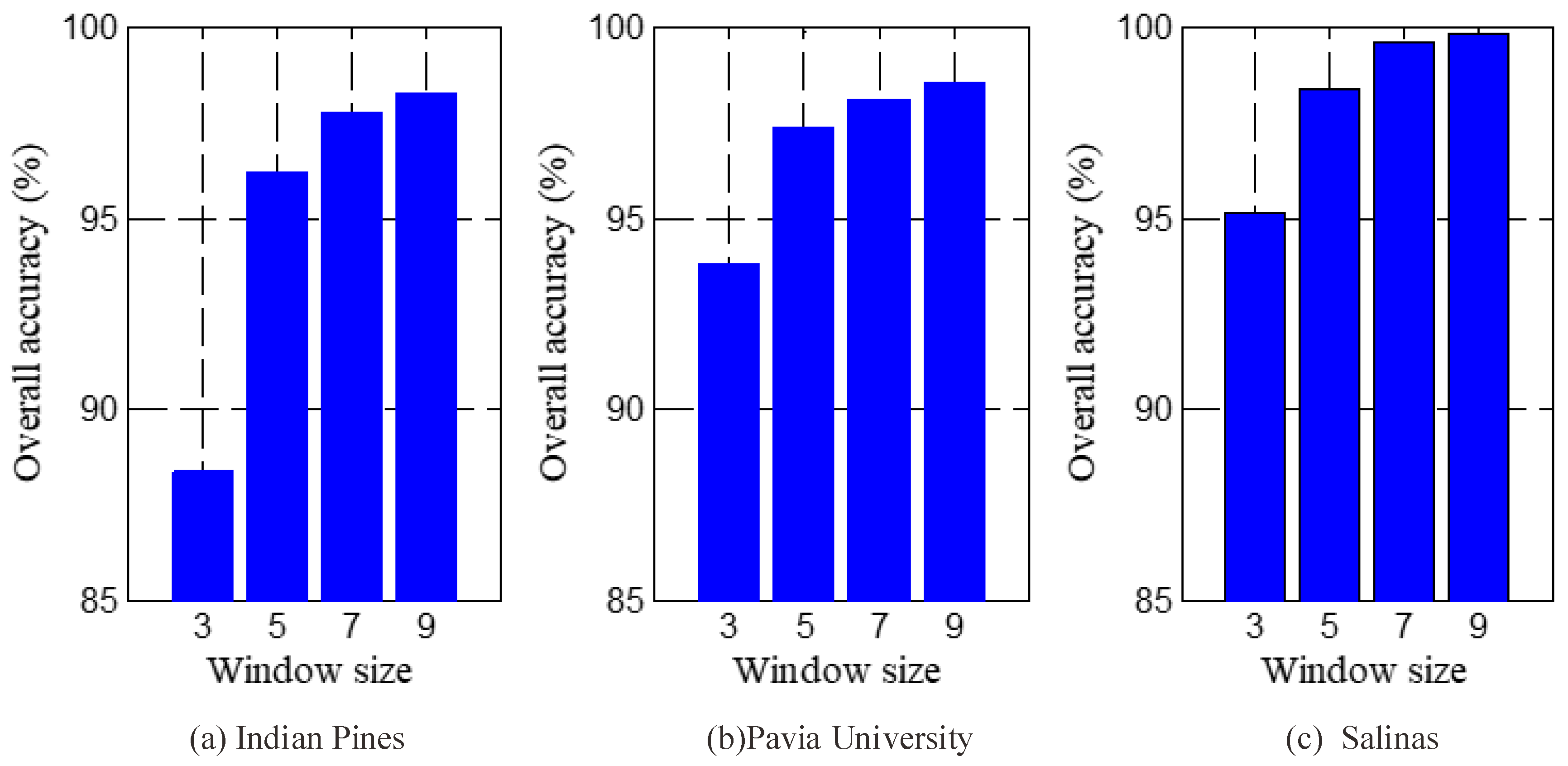
5.2. Discussion of the Spatial Size of Tensor Samples

The spatial fixed window criterion is employed to construct tensor samples in the proposed method. When the spatial fixed window criterion is concerned, the window size is an important issue. If a too small window is employed, each tensor sample may contain only a few pixel samples and the spatial region neighborhood information cannot be well preserved. On the other hand, a too large window may cause the pixel samples of different categories to be divided into the same tensor sample which may destroy the spatial structure consistency. Here, the effects of the window size on the classification accuracy are discussed experimentally and the results are illustrated in Figure 8. Specifically, we suppose the spatial window is a square with a side length of B. It can be observed from Figure 8 that, if a small spatial window is employed, such as 3, the classification performance is poor and with the increase of window size, the classification accuracy increases and then goes stabilized. The spatial window size is set as 9 × 9 in all the experiments.

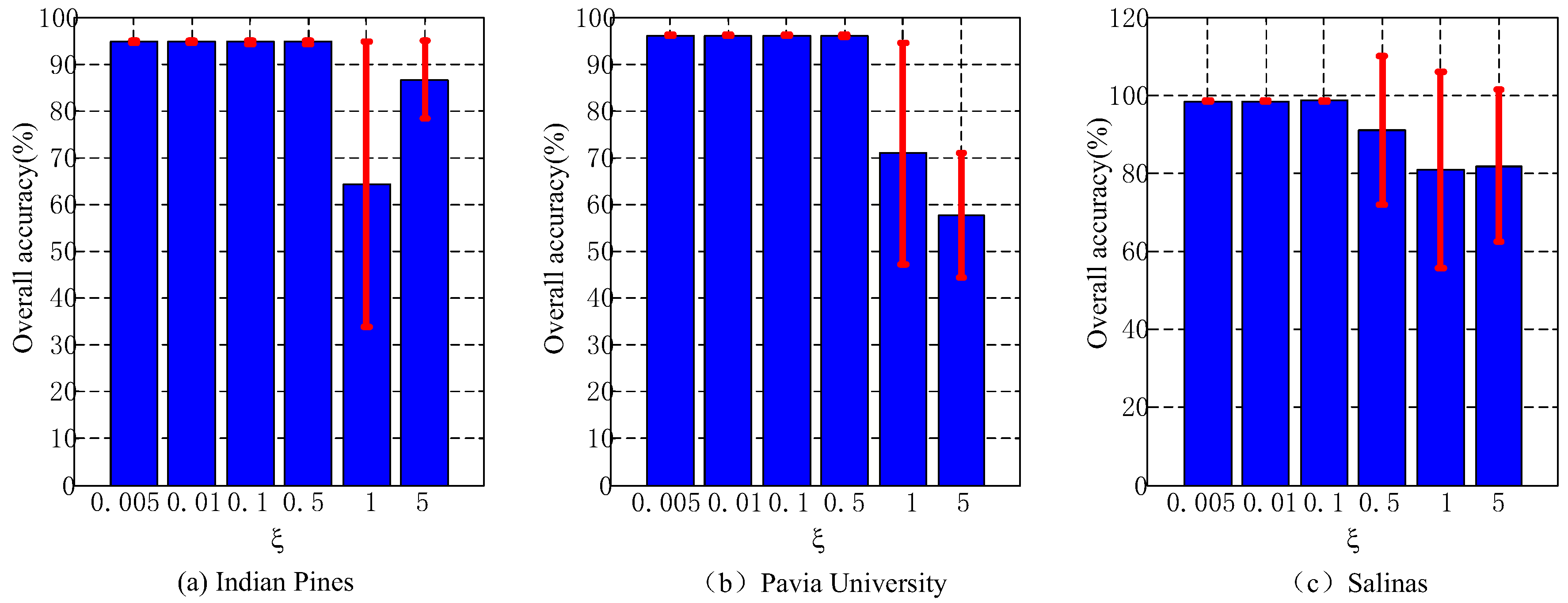
5.3. Discussion of the Parameter ξ

As the discussion above, parameter ξ is used to measure the effect of within class compactness and between class separation in tensor discriminant analysis model. Here, the effect of ξ in term of OA are discussed experimentally. Specifically, ξ varies from [0.005, 0.01, 0.05, 0.1, 1, 5] and the experimental results with SVM classifier are shown in Figure 9. It can be seen from Figure 9 that, when the value of ξ is small, such as 0.005, 0.01, 0.1, the proposed method can achieve the desirable classification performance and the corresponding variance is small. With larger ξ , the classification performance may degrade evidently and the corresponding variance may also increase, which suggests the proposed method cannot work steadily with a large ξ . So the parameter ξ is set as 0.01 in all these experiments.

6. Conclusions

A novel compact feature representation based tensor discriminative analysis model was proposed for hyperspectral images dimensionality reduction. Generally speaking, an ideal feature representation should be compact and discriminative. To this end, tensor low rank decomposition framework is employed in the proposed TDA-CFR to obtain a more compact feature representation which can eliminate the chaotic and conflicting information of the raw spectral bands. In addition, the tensor discriminant analysis which can preserve the original spatial region information and enhance the discriminant of the processed dataset is integrated to the compact feature representation model. Extensive experiments illustrate the superiority of TDA-CFR over the existing methods.
Final, there are still some issues which deserve further considered. In the proposed TDA-CFR, the spatial size of tensor samples are determined experimentally, how to construct tensor samples by a spatial window with adaptive size deserves further study. In addition, how to integrate the process of dimensionality reduction and the following tasks into one framework and make the results of dimensionality reduction more suitable for specific tasks requires further consideration.

Author Contributions

Methodology, J.A. and X.Z.; Resources, Y.G.; Validation, X.M. and Y.S.; Writing—original draft, J.A.; Writing—review & editing, X.Z.

Funding

This work is supported by Open Fund of Key Laboratory of Intelligent Perception and Image Understanding of Ministry of Education, Xidian University (Grant No. IPIU2019009), the State Key Program of National Natural Science of China (No. 61836009), the National Natural Science Foundation of China (Grant No. 61772400), the National Natural Science Foundation of China(No. 61801350), the China Postdoctoral Science Foundation Funded Project (No. 2018M633466), the China postdoctoral Innovative Talent Support Program (No. BX20180237) and the Natural Science Basic Research Program in Shaanxi Province of China (No. 2019JM-456.)

Conflicts of Interest

All the authors declare no conflict of interest.

References

  1. Chang, C.I. A Review of Virtual Dimensionality for Hyperspectral Imagery. IEEE J. Sel. Top. Appl. Earth Obs. Remote. Sens. 2018, 11, 1285–1305. [Google Scholar] [CrossRef]
  2. Harsanyi, J.C.; Chang, C. Hyperspectral image classification and dimensionality reduction: An orthogonal subspace projection approach. IEEE Trans. Geosci. Remote Sens. 1994, 32, 779–785. [Google Scholar] [CrossRef]
  3. Mohanty, R.; Happy, S.L.; Routray, A. A Semisupervised Spatial Spectral Regularized Manifold Local Scaling Cut With HGF for Dimensionality Reduction of Hyperspectral Images. IEEE Trans. Geosci. Remote. Sens. 2018, 57, 3423–3435. [Google Scholar] [CrossRef]
  4. Du, W.; Qiang, W.; Meng, L.; Hou, Q.; Ling, Z.; Ling, J. Semi-supervised dimension reduction based on hypergraph embedding for hyperspectral images. Int. J. Remote Sens. 2018, 39, 1696–1712. [Google Scholar] [CrossRef]
  5. Li, J.; Huang, X.; Gamba, P.; Bioucas-Dias, J.M.; Zhang, L.; Benediktsson, J.A.; Plaza, A. Multiple Feature Learning for Hyperspectral Image Classification. IEEE Trans. Geosci. Remote Sens. 2015, 53, 1592–1606. [Google Scholar] [CrossRef]
  6. Luo, F.; Bo, D.; Zhang, L.; Zhang, L.; Tao, D. Feature Learning Using Spatial-Spectral Hypergraph Discriminant Analysis for Hyperspectral Image. IEEE Trans. Cybern. 2019, 49, 2406–2419. [Google Scholar] [CrossRef] [PubMed]
  7. Cheng, G.; Zhenpeng, L.; Junwei, H.; Xiwen, Y.; Lei, G. Exploring Hierarchical Convolutional Features for Hyperspectral Image Classification. IEEE Trans. Geosci. Remote Sens. 2018, 56, 6712–6722. [Google Scholar] [CrossRef]
  8. Pal, M.; Foody, G.M. Feature Selection for Classification of Hyperspectral Data by SVM. IEEE Trans. Geosci. Remote Sens. 2010, 48, 2297–2307. [Google Scholar] [CrossRef] [Green Version]
  9. Zhang, W.; Li, X.; Zhao, L. Band Priority Index: A Feature Selection Framework for Hyperspectral Imagery. Remote Sens. 2018, 10, 1095. [Google Scholar] [CrossRef]
  10. Gong, C.; Zhou, P.; Han, J. RIFD-CNN: Rotation-Invariant and Fisher Discriminative Convolutional Neural Networks for Object Detection. In Proceedings of the 2016 IEEE Conference on Computer Vision and Pattern Recognition (CVPR), Las Vegas, NV, USA, 27–30 June 2016. [Google Scholar]
  11. Fraley, C.; Raftery, A.E. Model-Based Clustering, Discriminant Analysis, and Density Estimation. Publ. Am. Stat. Assoc. 2002, 97, 611–631. [Google Scholar] [CrossRef]
  12. Liu, Q.; Lu, H.; Ma, S. Improving kernel Fisher discriminant analysis for face recognition. Circuits Syst. Video Technol. IEEE Trans. 2004, 14, 42–49. [Google Scholar] [CrossRef]
  13. Prntland, A. Viewbased and modular eigenspaces for face recognition. In Proceedings of the 1994 IEEE Conference on Computer Vision and Pattern Recognition, Seattle, WA, USA, 21–23 June 1994; pp. 84–91. [Google Scholar]
  14. Kai, Z.; Min, W.; Yang, S.; Jiao, L. Spatial–Spectral-Graph-Regularized Low-Rank Tensor Decomposition for Multispectral and Hyperspectral Image Fusion. IEEE J. Sel. Top. Appl. Earth Obs. Remote. Sens. 2018, 11, 1030–1040. [Google Scholar]
  15. Qu, J.; Lei, J.; Li, Y.; Dong, W.; Zeng, Z.; Chen, D. Structure Tensor-Based Algorithm for Hyperspectral and Panchromatic Images Fusion. Remote Sens. 2018, 10, 373. [Google Scholar] [CrossRef]
  16. Xu, Y.; Wu, Z.; Chanussot, J.; Wei, Z. Nonlocal Patch Tensor Sparse Representation for Hyperspectral Image Super-Resolution. IEEE Trans. Image Process. 2019, 28, 3034–3047. [Google Scholar] [CrossRef] [PubMed]
  17. Velascoforero, S.; Angulo, J. Classification of hyperspectral images by tensor modeling and additive morphological decomposition. Pattern Recognit. 2013, 46, 566–577. [Google Scholar] [CrossRef] [Green Version]
  18. Yang, B.; Wang, B. Band-Wise Nonlinear Unmixing for Hyperspectral Imagery Using an Extended Multilinear Mixing Model. IEEE Trans. Geosci. Remote. Sens. 2018, 56, 6747–6762. [Google Scholar] [CrossRef]
  19. Zhang, L.; Zhang, L.; Tao, D.; Huang, X. Tensor Discriminative Locality Alignment for Hyperspectral Image Spectral-Spatial Feature Extraction. IEEE Trans. Geosci. Remote Sens. 2012, 51, 242–256. [Google Scholar] [CrossRef]
  20. Yan, S.; Xu, D.; Yang, Q.; Zhang, L.; Tang, X.; Zhang, H.J. Multilinear Discriminant Analysis for Face Recognition. IEEE Trans. Image Process. 2007, 16, 212–220. [Google Scholar] [CrossRef]
  21. Tao, D.; Li, X.; Wu, X.; Maybank, S.J. General tensor discriminant analysis and Gabor features for gait recognition. IEEE Trans. Pattern Anal. Mach. Intell. 2007, 29, 1700–1715. [Google Scholar] [CrossRef]
  22. Nie, F.; Xiang, S.; Song, Y.; Zhang, C. Extracting the optimal dimensionality for local tensor discriminant analysis. Pattern Recognit. 2009, 42, 105–114. [Google Scholar] [CrossRef]
  23. Zhong, Z.; Fan, B.; Duan, J.; Wang, L.; Ding, K.; Xiang, S.; Pan, C. Discriminant Tensor Spectral Spatial Feature Extraction for Hyperspectral Image Classification. IEEE Geosci. Remote Sens. Lett. 2017, 12, 1028–1032. [Google Scholar] [CrossRef]
  24. Zhou, P.; Han, J.; Cheng, G.; Zhang, B. Learning Compact and Discriminative Stacked Autoencoder for Hyperspectral Image Classification. IEEE Trans. Geosci. Remote. Sens. 2019, 57, 4823–4833. [Google Scholar] [CrossRef]
  25. Bandos, T.V.; Bruzzone, L.; Camps-Valls, G. Classification of Hyperspectral Images with Regularized Linear Discriminant Analysis. IEEE Trans. Geosci. Remote Sens. 2009, 47, 862–873. [Google Scholar] [CrossRef]
  26. Wang, H.; Wu, Q.; Shi, L.; Yu, Y.; Ahuja, N. Out-of-core tensor approximation of multi-dimensional matrices of visual data. ACM Trans. Graph. 2005, 24, 527–535. [Google Scholar] [CrossRef]
  27. Li, Q.; Schonfeld, D. Multilinear Discriminant Analysis for Higher-Order Tensor Data Classification. Pattern Anal. Mach. Intell. IEEE Trans. 2014, 36, 2524–2537. [Google Scholar]
  28. Lathauwer, L.D.; Moor, B.D.; Vandewalle, J. On the best rank-1 and rank-(R1, R2,...,RN ) approximation of higher-order tensor. SIAM J. Matrix Anal. Appl. 2000, 21, 1324–1342. [Google Scholar] [CrossRef]
  29. Hyperspectral Remote Sensing Scenes. Available online: http://www.ehu.eus/ccwintco/index.php?title=Hyperspectral_Remote_Sensing_Scenes (accessed on 4 April 2018).
  30. Li, W.; Liu, J.; Du, Q. Sparse and Low-Rank Graph for Discriminant Analysis of Hyperspectral Imagery. IEEE Trans. Geosci. Remote Sens. 2016, 54, 4094–4105. [Google Scholar] [CrossRef]
  31. Renard, N.; Bourennane, S.; Blanc-Talon, J. Denoising and Dimensionality Reduction Using Multilinear Tools for Hyperspectral Images. IEEE Geosci. Remote Sens. Lett. 2008, 5, 138–142. [Google Scholar] [CrossRef]
  32. An, J.; Zhang, X.; Jiao, L.C. Dimensionality Reduction Based on Group-Based Tensor Model for Hyperspectral Image Classification. IEEE Geosci. Remote Sens. Lett. 2016, 13, 1497–1501. [Google Scholar] [CrossRef]
  33. Pan, L.; Li, H.C.; Deng, Y.J.; Zhang, F.; Chen, X.D.; Du, Q. Hyperspectral Dimensionality Reduction by Tensor Sparse and Low-Rank Graph-Based Discriminant Analysis. Remote Sens. 2017, 9, 452. [Google Scholar] [CrossRef]
Figure 1. The flowchart of the proposed TDA-CFR.
Remotesensing 11 01822 g001
Figure 2. The compact representation of hyperspectral images.
Remotesensing 11 01822 g002
Figure 3. The classification maps on Indian Pines.
Remotesensing 11 01822 g003
Figure 4. The classification maps on Pavia University.
Remotesensing 11 01822 g004
Figure 5. The classification maps on Salinas.
Remotesensing 11 01822 g005
Figure 6. OA with SVM classifier versus the variation of reduced dimensionality.
Remotesensing 11 01822 g006
Figure 7. OA with SVM classifier versus the variation of the number of training samples for each class.
Remotesensing 11 01822 g007
Figure 8. OA with SVM classifier versus the variation of window size.
Remotesensing 11 01822 g008
Figure 9. The effect of parameter ξ .
Remotesensing 11 01822 g009
Table 1. Classification results on Indian Pines.
ClassOriginalLDASLGDAGTLRTDALRTATSLGDATDA-CFR
SVM1NNSVM1NNSVM1NNSVM1NNSVM1NNSVM1NNSVM1NNSVM1NN
172.71
±9.97
64.17
±9.7
73.33
±7.64
67.36
±10.97
76.6
±7.84
65.9
±8.81
90.42
±6.94
89.86
±8.03
75.76
±17.07
74.31
±13.72
85.14
±6.76
81.53
±6.08
95.21
±4.27
91.35
±7.16
96.46
±3.73
95.14
±5.17
284.3
±1.61
64.51
±1.86
80.37
±1.84
58.83
±5.61
80.66
±1.97
63.23
±2.02
90.38
±2.43
91.12
±2.01
87.45
±3.65
89.31
±2.75
91.02
±1.32
89.83
±1.58
93.45
±1.85
94.81
±1.55
97.56
±0.99
97.89
±0.65
376.61
±2.37
62.75
±2.41
66.91
±2.02
48.72
±6.06
76.1
±2.9
62.77
±2.52
90.42
±2.82
90.63
±2.73
82.56
±5.62
88.58
±3.97
85.84
±1.87
86.22
±2.08
92.75
±2.86
92.99
±2.29
98.34
±0.97
97.88
±0.87
471.11
±7
47.1
±6.31
64.71
±5.25
42.57
±9.07
68.56
±6.61
45.27
±5.39
87.6
±4.66
88.98
±3.57
69.22
±14.62
79.51
±6.5
85.68
±4.58
86.87
±4.12
92.38
±3.72
92.86
±3.55
96.43
±3.01
96.68
±1.87
593.71
±1.61
90.77
±1.78
92.38
±1.84
86.63
±4.1
93.06
±2.11
89.68
±2.21
95.59
±2.43
95.72
±2.51
92.58
±2.25
92.94
±2.85
97.01
±2.08
95.59
±2.22
95.91
±2.35
96.15
±1.83
98.16
±1.56
97.52
±1.64
696.31
±1.31
94.78
±1.55
95.9
±1.21
92.51
±2.12
95.84
±2.07
94.77
±1.64
94.79
±3.09
94.86
±3.08
95.74
±1.39
96.28
±2.08
99.51
±0.48
99.61
±0.37
97.94
±0.82
97.37
±1.65
99
±0.63
98.66
±0.86
777.39
±9.68
79.71
±17
73.83
±13.83
54.33
±16.67
80.43
±8.82
81.01
±8.36
100
±0
100
±0
60.87
±28
84.49
±13
80.58
±10
79.13
±10
85.00
±13.36
90.22
±8.79
94.49
±6.64
93.77
±7.75
898.35
±0.87
97.78
±1.07
98.33
±0.64
97.54
±1.38
97.93
±1.22
97.3
±1.47
98.13
±3.05
98.61
±2.69
98.06
±1.77
97.85
±1.56
99.85
±0.31
99.85
±0.28
99.85
±0.27
99.68
±0.38
99.97
±0.13
99.98
±0.07
972.96
±15.09
57.59
±11.61
73.96
±17.31
61.04
±20.01
67.41
±16.02
50.37
±14.41
33.89
±22.56
35.19
±18.33
18.33
±23.27
59.26
±17.99
86.67
±19.01
92.22
±11.26
79.44
±18.1
75.83
±15.94
81.67
±18.93
78.52
±18.35
1078.71
±1.79
73.95
±2.51
69.73
±2.48
56.64
±5.54
77.47
±3.28
72.27
±3.3
91.16
±3.51
90.88
±3.34
78.55
±6.14
88.88
±2.88
85.65
±2.87
90.23
±2.07
90.43
±1.99
91.84
±3.51
95.9
±2.13
96.88
±1.69
1184.12
±1.44
77.05
±1.3
82.87
±1.32
67.86
±3.34
80.94
±1.5
76.11
±1.48
99.4
±0.62
98.22
±0.88
91.96
±1.84
92.87
±2.18
89.38
±1.9
94.28
±1.06
95.07
±1.43
96.41
±0.99
98.69
±0.62
98.94
±0.48
1283.64
±2.51
57.13
±2.61
75.61
±2.72
62.65
±7.63
81.7
±3.48
56.15
±2.73
82.17
±3.76
81.7
±3.4
81.46
±7.5
84.35
±5.01
90.75
±2.47
89.08
±2.84
93.18
±2.92
94.12
±1.83
97.49
±1.34
97.13
±1.25
1398.88
±0.9
97.89
±1.54
98.84
±1.06
96.96
±3.7
98.56
±1.41
97.84
±1.74
93.33
±8.09
93.28
±8.15
92.11
±4.61
93.65
±5.21
99.88
±0.26
99.93
±0.18
97.95
±1.65
95.92
±3.00
98.67
±1.13
97.96
±1.48
1494.49
±1.51
93.64
±1.48
95.93
±1.21
92.81
±1.47
93.14
±1.93
93.51
±1.25
95.98
±2.38
96.63
±2.01
97.23
±1.25
96.62
±1.08
96.03
±1.61
98.44
±0.57
98.50
±0.72
98.84
±0.72
99.45
±0.62
99.65
±0.26
1561.05
±4.97
44.53
±3.78
71.79
±4.91
56.49
±6.43
61.3
±5.47
45.44
±3.83
93.51
±3.93
93.78
±3.67
87.55
±5.78
90.31
±4.22
86.36
±4.14
85.67
±3.45
93.67
±2.95
94.30
±3.65
98.76
±1.29
98.9
±0.98
1691.14
±4.43
91.06
±4.54
89.25
±4.37
78.25
±8.84
91.65
±4.49
90.51
±4.15
62
±13.27
59.96
±13.22
91.49
±6.04
91.88
±4.53
94.08
±5.08
92.94
±5.7
90.59
±7.06
89.53
±6.22
94.27
±6.17
93.33
±5.08
OA85.44
±0.41
76.27
±0.6
82.81
±0.51
70.56
±3.37
83.62
±0.62
75.55
±0.58
93.52
±0.66
93.44
±0.7
88.98
±2.07
91.54
±2.1
91.49
±0.7
93.07
±0.56
94.86
±1.02
95.55
±1.13
98.18
±0.3
98.26
±0.22
AA83.47
±1.1
74.65
±1.33
81.48
±1.87
70.08
±5.31
82.58
±1.44
73.88
±1.37
87.42
±1.87
87.46
±1.65
81.31
±4.47
87.57
±2.96
90.84
±1.2
91.34
±1.05
93.21
±1.70
93.26
±2.2
96.58
±1.43
96.18
±1.24
Kappa0.85
±0
0.76
±0.01
0.84
±0
0.73
±0.03
0.83
±0.01
0.75
±0.01
0.93
±0.01
0.93
±0.01
0.89
±0.02
0.91
±0.02
0.91
±0.01
0.93
±0.01
0.95
±0.01
0.95
±0.01
0.98
±0
0.98
±0
Table 2. Classification results on Pavia University.
ClassOriginalLDASLGDAGTLRTDALRTATSLGDATDA-CFR
SVM1NNSVM1NNSVM1NNSVM1NNSVM1NNSVM1NNSVM1NNSVM1NN
190.21
±0.63
75.76
±0.99
92.43
±0.44
85.62
±0.66
89.42
±0.9
78.05
±0.8
92.71
±1.6
95.01
±0.84
95.96
±1.25
95.54
±1.31
93.56
±0.67
96.71
±0.4
97.09
±0.72
93.51
±1.77
98.58
±0.49
98.03
±0.54
295.3
±0.36
94.91
±0.3
95.12
±0.25
93.54
±0.3
94.14
±0.41
94.3
±0.36
99.85
±0.13
99.41
±0.22
99.3
±0.34
99.89
±0.08
98.18
±0.23
99.51
±0.09
99.52
±0.16
99.84
±0.09
99.88
±0.07
99.98
±0.03
371.52
±1.65
59.97
±2.07
65.04
±1.42
66.63
±1.3
70.43
±2.41
61.48
±1.77
91.56
±2.04
94.97
±1.52
79.33
±3.4
90.37
±2.5
76.70
±1.41
91.70
±1.59
86.12
±2.31
90.93
±2.34
94.27
±1.6
96.51
±1.05
493.08
±0.73
84.5
±1.13
88.21
±0.68
85.88
±0.9
91.92
±1.13
83.8
±1.38
73.47
±2.39
78.62
±1.92
95.67
±0.88
93.02
±1.85
92.53
±0.79
94.02
±0.63
96.91
±0.88
94.22
±1.37
97.11
±0.44
94.56
±0.94
599.19
±0.41
99.31
±0.36
99.81
±0.18
99.74
±0.17
99.21
±0.55
99.3
±0.39
82.59
±2.17
93.45
±1.66
99.92
±0.11
99.88
±0.16
99.97
±0.06
99.9
±0.12
99.94
±0.12
99.98
±0.04
99.98
±0.04
99.91
±0.1
679.27
±1.18
56.95
±0.85
77.47
±0.87
69.62
±1.1
77.85
±1.2
57.03
±1.36
98.85
±0.5
99.64
±0.24
92.17
±2.8
99.44
±0.4
93.13
±0.79
99.63
±0.17
97.62
±0.87
98.75
±0.59
99.63
±0.27
99.96
±0.04
782.83
±1.38
77.86
±1.69
65.03
±2.86
76.31
±1.64
81.31
±2.49
76.85
±1.74
94.25
±1.43
97.1
±1.12
88.81
±4.7
91.58
±3
93.16
±1.67
96.65
±1.17
94.30
±1.72
96.56
±1.69
98.53
±0.82
99.11
±0.64
878.69
±1.74
76.75
±1.4
85.05
±1.05
73.17
±0.92
75.73
±1.26
75.24
±1.31
88.15
±1.89
92.72
±1.62
86.12
±2.66
90.65
±2.19
80.93
±1.03
88.05
±0.86
89.35
±2.06
91.23
±2.58
93.28
±1.3
96.27
±0.86
998.94
±0.27
92.24
±1.75
99.14
±0.33
96.54
±0.85
98.85
±0.28
92.93
±1.95
65.59
±3.09
77.01
±3.35
97.07
±1.07
90.83
±3.09
95.63
±1.32
96.67
±0.9
96.47
±1.82
80.91
±5.09
96.94
±1.15
90.95
±2.5
OA89.63
±0.21
82.89
±0.26
89.02
±0.14
85.51
±0.22
88.39
±0.25
82.87
±0.21
93.59
±0.41
95.53
±0.23
95.14
±0.59
96.86
±0.73
93.67
±0.14
97.11
±0.16
96.93
±0.41
96.54
±0.82
98.46
±0.16
98.51
±0.11
AA87.67
±0.29
79.81
±0.43
85.26
±0.36
83.01
±0.3
86.54
±0.43
79.89
±0.38
87.44
±0.62
91.99
±0.44
92.71
±0.94
94.58
±1.28
91.53
±0.26
95.87
±0.31
95.26
±0.66
93.99
±1.32
97.58
±0.29
97.25
±0.31
Kappa0.88
±0
0.8
±0
0.88
±0
0.85
±0
0.86
±0
0.8
±0
0.92
±0.01
0.95
±0
0.94
±0.01
0.96
±0.01
0.93
±0
0.97
±0
0.96
±0
0.96
±0.01
0.98
±0
0.98
±0
Table 3. Classification results on Salinas.
ClassOriginalLDASLGDAGTLRTDALRTATSLGDATDA-CFR
SVM1NNSVM1NNSVM1NNSVM1NNSVM1NNSVM1NNSVM1NNSVM1NN
199.61
±0.3
99.3
±0.24
99.93
±0.07
99.87
±0.15
99.47
±0.49
99.31
±0.31
98.3
±0.86
99.08
±0.64
99.4
±0.62
99.79
±0.22
99.91
±0.15
99.85
±0.16
99.97
±0.05
99.86
±0.07
99.98
±0.05
99.97
±0.05
299.76
±0.18
99.32
±0.24
99.96
±0.03
99.95
±0.03
99.69
±0.26
99.27
±0.26
98.75
±0.76
99.31
±0.57
99.77
±0.24
99.95
±0.09
100
±0.01
100
±0.01
100
±0
100
±0
100
±0
100
±0
399.73
±0.14
97.96
±0.64
99.78
±0.11
99.72
±0.11
99.57
±0.21
97.8
±0.7
98.43
±1.1
99.15
±0.7
99.92
±0.11
99.9
±0.16
99.94
±0.12
99.93
±0.09
99.90
±0.19
99.9
±0.12
100
±0
100
±0
499.25
±0.42
99.33
±0.33
99.26
±0.27
99.08
±0.39
99.31
±0.46
99.46
±0.22
92.01
±3.09
93.68
±2.41
98.52
±0.5
98.46
±0.72
97.49
±0.91
98.35
±0.69
96.68
±1.77
97.46
±1.43
98.84
±0.76
99.36
±0.39
599.19
±0.26
96.93
±0.64
99.1
±0.17
98.95
±0.23
98.75
±0.49
96.88
±0.56
95.56
±1.44
96.53
±1.09
99.43
±0.37
99.67
±0.29
98.3
±0.44
99.14
±0.31
98.48
±0.48
98.9
±0.79
99.19
±0.51
99.6
±0.18
699.83
±0.11
99.77
±0.12
99.95
±0.03
99.94
±0.03
99.76
±0.18
99.7
±0.17
96.9
±0.88
96.95
±0.91
99.99
±0.01
99.99
±0.01
99.97
±0.03
99.95
±0.03
99.99
±0.01
100
±0
100
±0.01
100
±0.01
799.57
±0.18
99.44
±0.17
99.94
±0.04
99.91
±0.06
99.65
±0.15
99.5
±0.15
97.5
±1.04
97.41
±0.9
99.75
±0.27
99.82
±0.17
99.99
±0.01
99.99
±0.03
99.99
±0.01
99.98
±0.02
100
±0.01
99.99
±0.03
883.54
±0.88
77.74
±0.84
89.06
±0.56
79
±0.73
87.88
±0.66
77.36
±0.67
99.54
±0.18
99.32
±0.27
92.51
±1.06
99.16
±0.4
93.03
±0.72
94.26
±0.32
95.76
±1.08
95.75
±2.45
99.68
±0.15
99.86
±0.08
999.83
±0.14
99.11
±0.31
99.91
±0.08
99.76
±0.13
99.45
±0.34
99.04
±0.35
99.15
±0.58
99.55
±0.36
99.99
±0.03
99.99
±0.03
99.84
±0.13
99.92
±0.05
99.98
±0.01
99.99
±0.02
100
±0
100
±0
1097.31
±0.56
94.74
±0.65
98.09
±0.32
97.84
±0.35
96.87
±0.58
94.51
±0.73
97.47
±0.9
97.66
±0.74
99.49
±0.31
99.69
±0.26
99.22
±0.28
99.01
±0.24
99.50
±0.64
99.45
±0.38
99.96
±0.12
99.92
±0.24
1199.16
±0.54
98.84
±0.73
99.14
±0.4
98.26
±0.52
98.92
±0.82
98.59
±0.83
95.27
±2.34
95.16
±2.29
99.86
±0.28
99.81
±0.35
99.59
±0.32
99.03
±0.47
99.93
±0.09
99.93
±0.12
99.99
±0.04
100
±0
1299.9
±0.12
99.81
±0.12
99.76
±0.16
99.65
±0.21
99.87
±0.16
99.8
±0.21
95.77
±1.67
95.66
±1.68
99.91
±0.2
99.97
±0.13
99.87
±0.14
99.6
±0.2
99.96
±0.06
99.93
±0.12
100
±0
100
±0.01
1399.17
±0.66
97.79
±0.61
99.05
±0.41
98.95
±0.28
99.22
±0.66
97.85
±0.58
89.39
±3.47
89.13
±3.85
99.7
±0.39
99.94
±0.16
99.41
±0.34
98.95
±0.52
99.76
±0.29
99.48
±0.62
99.88
±0.18
99.96
±0.1
1497.75
±0.95
95.04
±1.41
97.71
±0.56
97
±0.9
98.09
±0.68
95.5
±0.87
88.72
±3.66
87.6
±3.69
99.28
±0.74
99.71
±0.49
99.04
±0.48
98.54
±0.69
99.51
±0.31
99.57
±0.33
99.88
±0.19
99.85
±0.22
1575.63
±0.9
67.6
±1.08
66.09
±0.84
70.3
±1.26
78.65
±0.78
67.57
±1.12
99
±0.4
98.95
±0.34
83.4
±2.86
99.23
±0.53
80.47
±1.13
91.94
±0.58
93.34
±2.01
93.64
±3.78
99.32
±0.28
99.85
±0.09
1698.72
±0.46
98.15
±0.69
99.43
±0.31
99.44
±0.29
98.71
±0.46
98.3
±0.44
98.07
±0.76
98.86
±0.74
99.94
±0.16
99.92
±0.11
99.35
±0.41
99.26
±0.47
99.92
±0.13
99.83
±0.28
99.92
±0.19
99.9
±0.19
OA92.85
±0.22
90
±0.2
92.85
±0.07
91.23
±0.17
94.06
±0.13
89.89
±0.19
97.79
±0.32
97.97
±0.22
96.03
±0.53
99.6
±0.19
95.64
±0.16
97.45
±0.12
98.00
±0.49
98.07
±1.04
99.76
±0.06
99.9
±0.03
AA96.75
±0.14
95.06
±0.14
96.63
±0.06
96.1
±0.09
97.12
±0.1
95.03
±0.14
96.24
±0.57
96.5
±0.47
98.18
±0.25
99.69
±0.14
97.84
±0.11
98.61
±0.09
98.92
±0.24
98.98
±0.49
99.79
±0.06
99.89
±0.05
Kappa0.93
±0
0.9
±0
0.94
±0
0.92
±0
0.94
±0
0.9
±0
0.98
±0
0.98
±0
0.96
±0.01
1
±0
0.96
±0
0.97
±0
0.98
±0
0.98
±0.01
1
±0
1
±0
Table 4. The running time on three hyperspectral images (in seconds).
OriginalLDASLGDAGTLRTDALRTATSLGDATDA-CFR
Indian Pines1.891.021.733.254.982.7210.545.02
Pavia University10.057.525.5710.3667.065.6962.3568.34
Salinas18.0213.467.8213.7175.629.14156.2578.02

