Chlorophyll Concentration Response to the Typhoon Wind-Pump Induced Upper Ocean Processes Considering Air–Sea Heat Exchange

1
Guangdong Key Laboratory of Ocean Remote Sensing (LORS), State Key Laboratory of Tropical Oceanography (LTO), South China Sea Institute of Oceanology, Chinese Academy of Sciences, Guangzhou 510301, China
2
University of Chinese Academy of Sciences, Beijing 100049, China
3
Marine Hydrophysical Institute, Russian Academy of Sciences, 299011 Sevastopol, Russia
*
Author to whom correspondence should be addressed.
Remote Sens. 2019, 11(15), 1825; https://0-doi-org.brum.beds.ac.uk/10.3390/rs11151825
Submission received: 10 June 2019
/
Revised: 27 July 2019
/
Accepted: 1 August 2019
/
Published: 4 August 2019
(This article belongs to the Special Issue Tropical Cyclones Remote Sensing and Data Assimilation)
Abstract
:The typhoon Wind-Pump induced upwelling and cold eddy often promote the significant growth of phytoplankton after the typhoon. However, the importance of eddy-pumping and wind-driven upwelling on the sea surface chlorophyll a concentration (Chl-a) during the typhoon are still not clearly distinguished. In addition, the air–sea heat flux exchange is closely related to the upper ocean processes, but few studies have discussed its role in the sea surface Chl-a variations under typhoon conditions. Based on the cruise data, remote sensing data, and model data, this paper analyzes the contribution of the vertical motion caused by the eddy-pumping upwelling and Ekman pumping upwelling on the surface Chl-a, and quantitatively analyzes the influence of air–sea heat exchange on the surface Chl-a after the typhoon Linfa over the northeastern South China Sea (NSCS) in 2009. The results reveal the Wind Pump impacts on upper ocean processes: (1) The euphotic layer-integrated Chl-a increased after the typhoon, and the increasing of the surface Chl-a was not only the uplift of the deeper waters with high Chl-a but also the growth of the phytoplankton; (2) The Net Heat Flux (air–sea heat exchange) played a major role in controlling the upper ocean physical processes through cooling the SST and indirectly increased the surface Chl-a until two weeks after the typhoon; (3) the typhoon-induced cyclonic eddy was the most important physical process in increasing the surface Chl-a rather than the Ekman pumping and wind-stirring mixing after typhoon; (4) the spatial shift between the surface Chl-a blooms and the typhoon-induced cyclonic eddy could be due to the Ekman transport; (5) nutrients uplifting and adequate light were two major biochemical elements supplying for the growth of surface phytoplankton.

1. Introduction
Chlorophyll a concentration (Chl-a) is an important index of phytoplankton biomass and the main marine green photosynthetic pigment, and plays an important role in the process of relevance to marine atmospheric carbon cycle, of material cycle and energy conversion, environment monitoring, ocean currents, fishery management, and so on [1,2]. Although phytoplankton biomass in the oceans only amounts to 1–2% of the total global plant carbon, these organisms collectively fix approximately 40% of the global total carbon [1,3].
The northeastern South China Sea (NSCS) is generally stratified, tropical, and oligotrophic with low phytoplankton biomass and frequent mesoscale processes, and it is frequently influenced by the tropical cyclones during the summer time [4]. Tropical cyclones have important “Wind Pump” impact on transporting and increasing the surface and subsurface Chl-a in oligotrophic ocean waters [5,6,7,8] through uplifting the nutrients by strong vertical mixing, upwelling, entrainment, as well as near inertial wave on the upper ocean layer, especially on the right-hand side of the storm track in the Northern Hemisphere [2,9,10]. Typhoons with slower translation speeds and stronger wind speeds have greater impact on Chl-a and the translation speeds play the more crucial role [4,11]. Tropical cyclones can also induce cyclone eddies (or reduce anti-cyclone eddies), and these eddy-pumping upwelling can further increase the surface and subsurface Chl-a [4,12]. These typhoon wind-driven physical processes and air–sea exchanges that subsequently affect the ocean’s ecological status is defined as the “Wind Pump” [2,4,7,8,10,11].
Biochemical conditions are essential in affecting the Chl-a through affecting its carbon/chlorophyll ratios [1,13]. Upwelling of the nutrient-rich waters from the deeper layer is the principal source of nutrients fueling the phytoplankton especially over the oligotrophic ocean like the NSCS [1,4]. The nitrogen is the major nutrient element limiting phytoplankton biomass throughout most of the world oceans [1,14]. Light is another important biochemical factor supporting the growth of the phytoplankton, and most of the chlorophyll is concentrated in the euphotic [1]. The depth of the upper mixed layer relative to the depth of the euphotic zone is critical to the formation of phytoplankton blooms [1]. In principle, the euphotic zone and nutrients can be influenced by physical process, especially after the passage of tropical cyclones [2,13].
Many studies have been done on the effect of typhoons and mesoscale eddies on the Chl-a [2,4,15], but few studies have clearly distinguished the contribution of the wind-stirring mixing, the Ekman pumping upwelling, and the eddy-pumping upwelling in the upper ocean after the typhoon. The air–sea exchange is closely related to the upper marine conditions, and the ocean is the main source of energy for the tropical cyclones [16,17]. However, the air–sea exchange under typhoon conditions and its role in the upper ocean Chl-a during the typhoon remain largely unknown. Based on the in-situ data, satellite remote sensing data and model data, this paper analyzed the contribution of the wind-induced mixing and upwelling and the eddy-induced upwelling on the surface Chl-a, and quantitatively analyzed the effect of air–sea exchange on the surface Chl-a.
This paper is organized as follows. The data and methodology are presented in Section 2. The in-situ observations, satellite remote sensing data over the study area during the typhoon are examined in Section 3. The temporal variability of Chl-a induced by the typhoon Wind Pump, physical processes (especially the Ekman pumping and the mesoscale eddies), the net heat flux, and the biochemical processes influenced by the typhoon Linfa are discussed in Section 4. Conclusions are presented in Section 5.
2. Materials and Methods
2.1. Typhoon Data
The typhoon data was obtained from the Japan Meteorological website with a time resolution of 6 h (http://agora.ex.nii.ac.jp/digital-typhoon/), including the location of the typhoon center, the maximum sustained wind speed (MWS) at 10 m on the sea surface, the typhoon status, and the satellite image. The average translation speed of the typhoon Linfa in 2009 was estimated by dividing the distance with the time between two adjacent positions of the typhoon centers.
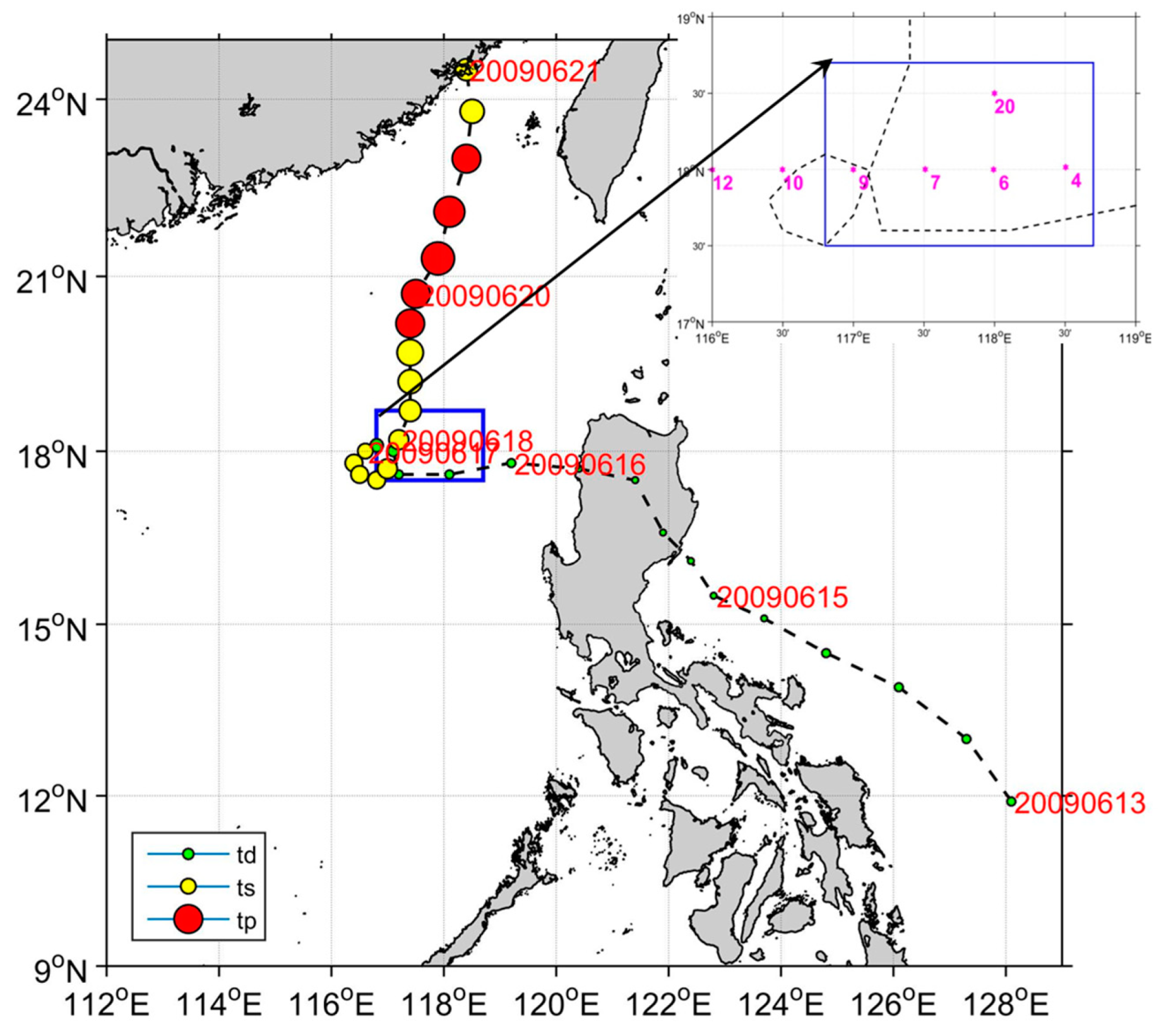
The typhoon Linfa originated from a tropical depression of the Northwest Pacific on 13 June 2009, and moved northwestwards to the Philippines on 15 June (MWS of ~28 km/h) (Figure 1). It moved westwards and entered the South China Sea on 16 June with MWS of ~28 km/h and the average translation speed of ~5.1 m/s. It then intensified and looped over the study area (116–117° E and 17–18° N) at 17–18 June, and was classified as a severe tropical storm with MWS of ~83 km/h and the average translation speed of ~1.5 m/s. Linfa then moved northwards and finally reached its peak strength as a typhoon with MWS of ~139 km/h on 20 June, and made a landfall on 21 June.
2.2. Remote Sensing Data and Model Data
The 8-day average rainfall data was calculated from the daily data obtained from WindSat with a spatial resolution of 0.25° × 0.25° (http://www.remss.com). The 8-day average of wind field data (wind speed) and wind stress data at 10 m above the sea level were calculated from the daily data extracted from the Ifremer (ftp.ifremer.fr/ifremer/cersat/products/gridded/), with a spatial resolution of 0.25° × 0.25°. The 8-day average Sea Surface Temperature (SST) was calculated from the daily SST obtained from the GHRSST OSTIA with a spatial resolution of 5 × 5 km (http://poet.jpl.nasa.gov). The 8-day average sea surface Chlorophyll a concentration (Chl-a) was merged using the MODIS Aqua and MODIS Terra L3 products (http://oceancolor.gsfc.nasa.gov/) with a spatial resolution of 4 × 4 km. The 8-day average sea level anomaly (SLA) data was calculated from the daily SLA extracted from AVISO with a spatial resolution of 0.25° × 0.25° (http://marine.copernicus.eu/). The 8-day average sea surface geostrophic currents data (geo-SSCs) was calculated from the daily geo-SSCs obtained from the Globcurrent with a spatial resolution of 0.25° × 0.25° (http://globcurrent.ifremer.fr/). The 8-day average sea surface net heat flux (NHF), latent heat flux (LHF), sensible heat flux (SHF), longwave radiation flux (LWRF), and shortwave radiation flux (SWRF) data were calculated from the daily NHF, LHF, SHF, LWRF, and SWRF extracted from Woods Hole Oceanographic Institute’s (WHOI) objectively analyzed air–sea heat fluxes data set with a spatial resolution of 1° × 1° (http://oaflux.whoi.edu/).
2.3. In Situ Data
The cruise data of potential temperature, salinity, and potential density data were conducted from the field program organized by the South China Sea Institute of Oceanography (SCSIO, Guangzhou, China), Chinese Academy of Science on 16–17 June 2009. The potential temperature, salinity, and potential density were measured and recorded every 1 s with a SEACAT CTD (SBE21, Sea-Bird Co., Bellevue, WA, USA) along the cruise tracks (Figure 1). The section at 18° N including Stations 2–4, 6, 7, 9, 10, and 12 from the east to the west, and intersects with Linfa over Stations 9 and 10. Station 20 is located at the same longitude as Station 6 but with a difference of ~0.5° at the latitude. All the cruise data collected in this study were at depths from surface to 200 m.
2.4. Methods
The Ekman pumping velocity (EPV) is calculated from the 8-days average ASCAT sea surface wind stress () data at 10 m above the sea level (positive indicates upwards) [10]:
where is the Coriolis parameter, is the density of sea water (refers to 1025.0 kg/m3).
The surface layer mixing caused by wind stirring may break through the stratification layer and bring the surface nutrients up to the surface layer [9,18]. The wind stirring-induced mixing () is given by [19]:
where (=1.3 kg/m3) is the air density, = 10−3 × (0.6 + 0.07 ) is the drag coefficient, and is the wind speed at 10 m height above the sea surface as derived from the ASCAT wind product.
Formula for calculating SST changes caused by sea surface net heat flux (NHF) is given by [20]:
where is the density of sea water (refers to 1025.0 kg/m3), is the specific heat of constant pressure seawater (4.2 × 10³ J/(Kg °C)), is the depth of the mixed layer, and is the net heat flux.
The mixed layer depth () is defined as the depth of the density gradient first exceeding 0.01 kg/m4, estimated from the temperature curve of the CTD [21].
The depth of the euphotic zone () is defined as the depth at which the photon flux equals 1% of the flux measured just above the air–sea interface [22]:
where is the total Chl-a at the sea surface (0 m).
In stratified waters, for surface Chl-a ≤ 1 mg/m3, an assessment of the column-integrated Chl-a based on the surface Chl-a was used [23]:
where represents the column-integrated Chl-a within the euphotic layer, and the represents the surface Chl-a.
3. Results
3.1. Distribution of the Surface Chl-a
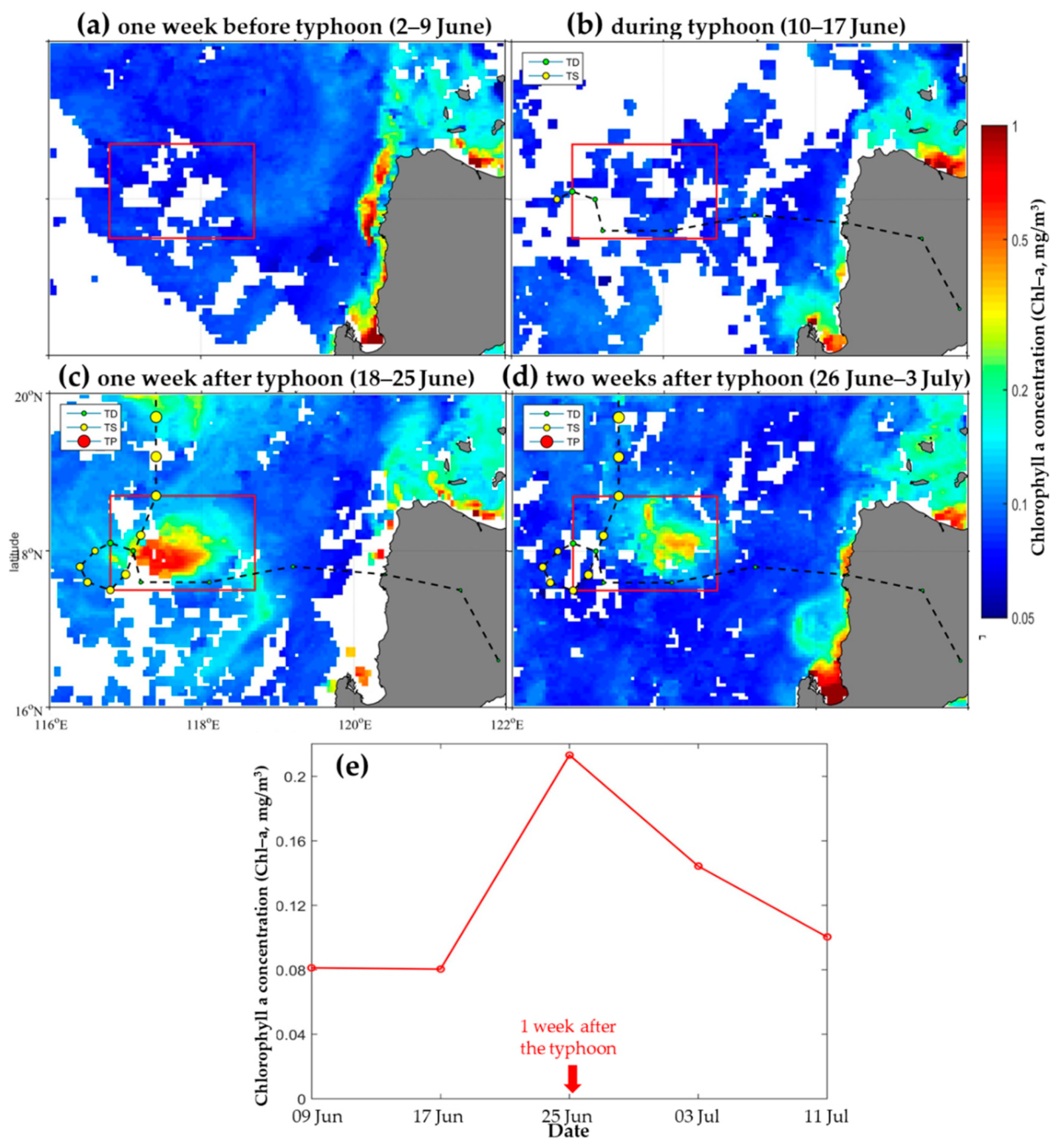
The changes of the surface chlorophyll a concentration (Chl-a) in the study area can be analyzed from the remote sensing data in Figure 2 regardless of some data missing (white pixels) due to the thick cloud cover. The sea surface Chl-a was generally low (average ~0.08 mg/m3) one week before the typhoon Linfa in the study area (2–6 June, Figure 2a). The surface Chl-a showed little change with an area average value of ~0.08 mg/m3 in the study during the Linfa passage (10–17 June, Figure 2b,e). The surface Chl-a increased significantly in the study area with area average value of ~0.22 mg/m3 one week after the typhoon (18–25 June, Figure 2c,e), which was more than twice of that before the typhoon. This significant surface Chl-a bloom presented a cyclonic pattern with the maximum Chl-a of ~0.5 mg/m3. The surface Chl-a gradually decreased in the study area with the area average value of ~0.14 mg/m3 two weeks after the typhoon (26 June–3 July, Figure 2d,e), and its cyclonic pattern disappeared. The area average surface Chl-a in the study area continued decreasing (~0.1 mg/m3) and basically restored to the pre-typhoon level three weeks after the typhoon (4–11 July, Figure 2e).
3.2. Remote Sensing Data of Rainfall, SST, and geo-SSCs
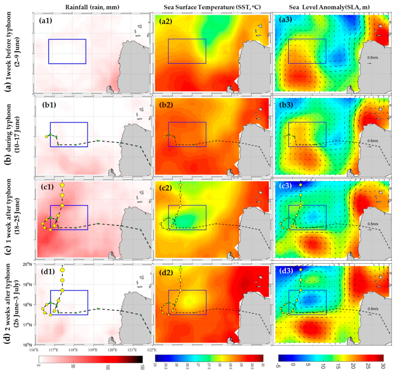
One week before the typhoon Linfa (Figure 3), there is rare rainfall (Figure 3a1), relatively high sea surface temperature (SST, area average of ~28.4 °C, Figure 3a2), and a relatively high sea level anomaly (SLA, area average of ~17 cm, Figure 3a3) with a southeastwards wind in the study area (blue box). Linfa entered the study area on 16 June 2009. There was still rare rainfall and the SLA showed slight decrease (Figure 3b), but the SST increased significantly (area average of ~0.5 °C, Figure 3b2) and the geo-SSCs showed an anti-cyclonic pattern due to the extension of the anti-cyclonic eddy at the south of the study area (Figure 3b3) during Linfa. One week after the typhoon entered the study area (Figure 3), rainfall increased significantly with a left-side bias (area average of ~55 mm (Figure 3c1), SST decreased significantly with a right-side bias (area average of ~27.5 °C, Figure 3c2), and the SLA decreased significantly (area average of ~7 cm) with a clearly cyclonic geo-SSCs pattern at the center of the study area (to the west of the typhoon looping area, Figure 3c3). Two weeks after the typhoon in the study area, rainfall decreased and basically restored to the pre-typhoon level (Figure 3d1), SST increased but still presented a cooling pattern (area average of ~28 °C, Figure 3d2) where the SLA continued decreasing and the cyclonic geo-SSCs enhanced (Figure 3d3). In addition, before and after the typhoon, there was a strong anti-cyclonic geo-SSCs pattern and high SLA southern outside of the study area.
Figure 3 indicates that there was a cyclonic eddy eastern outside of the study area before the typhoon (Figure 3a3) but this cyclonic eddy disappeared after the typhoon (Figure 3c3,d3). There was a pre-typhoon anti-cyclonic warm eddy southern outside of the study area, and its intensity weakened and size reduced during the Linfa but recovered after the typhoon (Figure 3). Moreover, the typhoon induced a cyclonic cold eddy at the center of the study area after its passage and this cyclonic eddy continued enhancing even two weeks after the typhoon (Figure 3c3,d3).
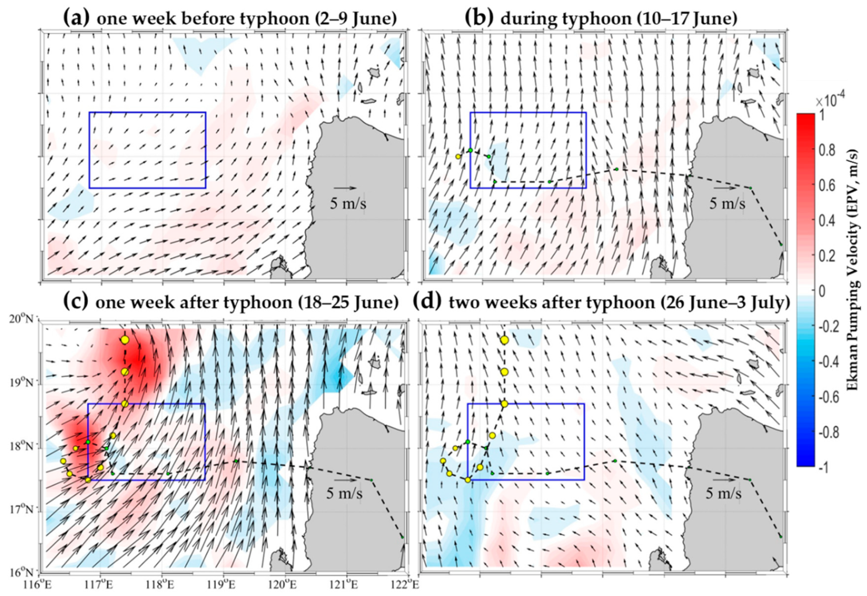
3.3. Distribution of the Wind and Wind Stress
One week before the typhoon (Figure 4a), the Ekman pumping velocity (EPV) was weak (<|0.5 × 10⁻⁵| m/s) in the study area, and it presented a southwest wind in the whole study area with an average wind speed of ~2.2 m/s. The EPV presented little change in the study area during the typhoon when the typhoon Linfa started looping at the west part of the study area (Figure 4b), but the wind intensified significantly (area average of ~3.3 m/s) and turned northwards. The EPV over the western study area increased significantly (area average of ~5 × 10⁻⁵ m/s) due to the looping of Linfa, and the EPV presented slight increase in the rest of the study area (area average of ~2.5 × 10⁻⁵ m/s) one week after the typhoon (Figure 4c). The intensity of the wind continued increasing (with maximum wind speed of ~8 m/ s) and presented a cyclonic pattern along the typhoon track during this period (Figure 4c). The EPV and wind speed in the study area gradually recovered to the pre-typhoon level (area average of <1 × 10⁻⁵ m/s and ~2.2 m/s, respectively) two weeks after the typhoon (Figure 4d), and the wind direction changed into southeastwards. Figure 4 shows that Linfa induced strong EPVs on the western study area due to its looping and then generated stronger Ekman pumping upwelling in the west side than in the rest of the study region such as the middle area where the post-typhoon cyclonic cold eddy occurred.
3.4. Daily Distribution of the Chl-a, EPV, and SLA
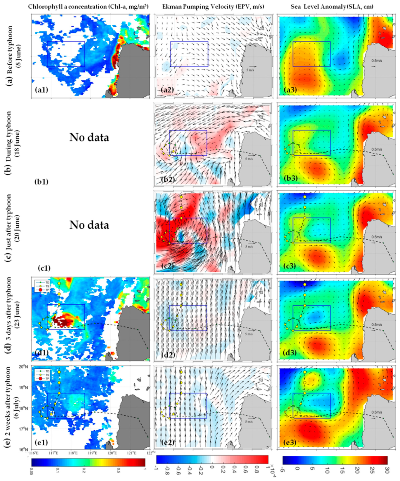
Figure 5 shows the daily distribution of the Chl-a, EPV, and SLA before and after the typhoon over the study area. Ten days before the typhoon (8 June, Figure 5a), the Chl-a was low (<0.14 mg/m3) with weak Ekman pumping velocity (EPV, <|1 × 10⁻⁵| m/s) and high SLA (~16 cm) in the study area, and the study area was occupied by an anti-cyclonic eddy which center located at the south of the study area while a cyclonic eddy located at the east of the study area. During the looping of the Linfa (18 June, Figure 5b) in the study area, the EPV increased up to ~2.5 × 10⁻⁵ m/s in the study area with a cyclonic pattern wind field in the east of the study area, the pre-existed cyclonic eddy east of the study area disappeared (SLA decreased to ~5 cm), and the anti-cyclonic eddy reduced to the south of the study area causing the disappeared of the decrease of the SLA in the study area. Right after the passage of the typhoon Linfa (20 June, Figure 5c), EPV significantly increased inside (~6 × 10⁻⁵ m/s) and especially around the study area (>6 × 10⁻⁵ m/s) with a cyclonic wind field, which coincided with the gradually generated cyclonic geo-SSCs and the decrease of the SLA in the study area. Three days after the typhoon (23 June, Figure 5d) in the study area, the EPV recovered to the pre-typhoon level (<|1.5 × 10⁻⁵| m/s) with a relatively stronger northeastward wind speed, and the cyclonic eddy enhanced with a significant surface alga bloom (>0.6 mg/m3), a lower SLA, and a stronger cyclonic geo-SSCs. Two weeks after the typhoon (6 July, Figure 5e) in the study area, the EPV and wind vectors maintained the pre-typhoon level (<|1 × 10⁻⁵| m/s, ~3m/s, respectively) with a northeastward wind direction, the cyclonic eddy kept its intensity as that of three days after the typhoon and moved eastward, and the Chl-a (~0.2 mg/m3) gradually restored to the pre-typhoon level (<0.14 mg/m3).
Figure 5 demonstrates that the cyclonic eddy was generated by the typhoon rather than the westward propagating of the pre-existed cyclonic eddy east of the study area, as wind stress curl coincided with the eddy just one day after the typhoon Linfa (Figure 5c) and no significant cyclonic eddy was found in the study area or east of the study area during the typhoon (Figure 5b).
3.5. Distribution of the In Situ Temperature and Salinity Profiles
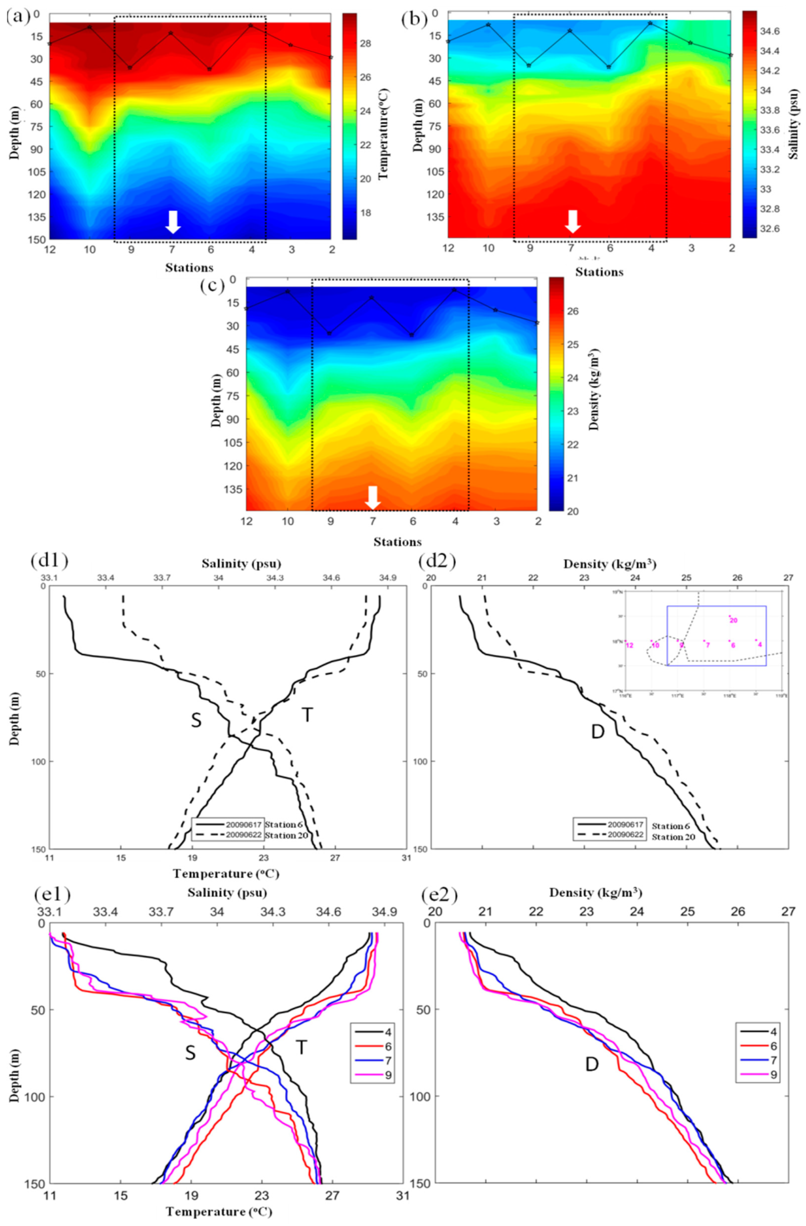
The in situ temperature, salinity, and density profiles along the 18° N section one day before and during the typhoon (16–17 June, 2009, Figure 6a,b) showed that the water mass with relatively high temperature (>28.5 °C) and relatively low salinity (<33.4 psu) occurred at Stations 9, 10, and 12 one day before the typhoon, and the water mass with relatively low temperature (<28.3 °C) and relatively high salinity (>33.6 psu) occurred at Stations 2–4 during the typhoon. The combination of low temperature and high salinity in the upper layer (~0–150 m) and shallow MLD centered at Station 3 (119° E, 18° N) is an indication of the pre-typhoon relatively strong upwelling east outside of the study area (Figure 3a3, Figure 6a,b). The low temperature and high salinity in the deeper layer (~75–150 m) with shallow MLD located at Station 7 (117.5° E, 18° N) also indicated an upwelling at deeper layer (~75–150 m) at the center of the study area during the typhoon where the post-typhoon maximum surface Chl-a and the post-typhoon low SLA occurred (Figure 3c3, Figure 6a,b).
Stations 6 and 20 are the CTD stations during (17 June, 2009) and three–four days after the typhoon (22 June, 2009), and they are basically located at the same longitude (117.5 °E) with their distance <50 km. The temperature and salinity profiles of these two stations are compared to reveal the possible upper ocean physical processes during and after the typhoon Linfa (Figure 6d1,d2). The observed temperature and salinity at Station 6 during the typhoon were vertically more uniform than the post-typhoon conditions at Station 20 within the surface mixed layer, and the density at Station 6 during typhoon had an uplift comparing with post-typhoon conditions at Station 20 from ~75–150 m. These conditions indicate strong vertical mixing during the typhoon and upwelling occurrence in ~0–150 m after the typhoon over the study area (Figure 6), and these were consistent with the typhoon-induced cyclonic eddy with center located at the same position as Station 6 which demonstrated by Figure 3c.
4. Discussion
4.1. The Increase of the Surface and Euphotic Layer-Integrated Chl-a
The typhoon-induced surface Chl-a increasing can result from the uplift of the higher Chl-a water at deeper layer to the surface and the upwards nutrients supplying for the growth of the phytoplankton [4,24]. It has documented that only half of the typhoons generated the Chl-a blooms and contributed to the marine primary productivity [4]. An assessment of the column-integrated Chl-a based on the surface Chl-a was used according to Formula (5) [23].
The average surface Chl-a () and the euphotic layer-integrated Chl-a () over the study region one week before the typhoon (0.08 mg/m3, 10.90 mg/m2, respectively) were similar to that at the center of the typhoon-induced cyclonic eddy or Station 7 (0.08 mg/m3, 10.64 mg/m2, respectively), which were also consistent with Liu’s finding that the surface Chl-a and the column-integrated Chl-a within 0–100 m were ~0.1mg/m3 and ~10 mg/m2, respectively, according to the cruise data over the NSCS at summer without typhoons [25]. The increased ~83% over the study region (18.33 mg/m2) and ~178% at the center of the typhoon-induced cyclonic eddy (CE center, 27.79 mg/m2) one week after the typhoon. The and gradually recovered two weeks after the typhoon. These indicated that the increase of the surface Chl-a after typhoon was not only the uplift of the high Chl-a water from deeper layer but mainly the growth of the surface phytoplankton [4,24], and the increase of the Chl-a not only occurred in the surface but also within the water column in the euphotic layer.
The euphotic layer-integrated Chl-a was divided with the euphotic layer depth (ELD) to roughly estimate the Chl-a entrainment in the ELD (Table 1). The Chl-a entrainment in the center of the typhoon-induced eddy (0.13 mg/m3) is similar to the study area averaged Chl-a entrainment (0.13 mg/m3), which proves the accuracy of the calculation. The Chl-a entrainment in the center of the typhoon-induced eddy (Station 7, 0.61 mg/m3) is much bigger than that of the study area (0.30 mg/m3) one week after the typhoon, which indicated that the eddy-pumping played a major role in the growth of the surface and the euphotic layer-integrated Chl-a (Table 1 and Table 2). Two weeks after the typhoon (6 July), the Chl-a entrainment at Station 7 (0.22 mg/m3) decreased to nearly twice as pre-typhoon level (0.13 mg/m3) and was similar to the averaged value of the study area (0.21 mg/m3), which coincided with the eastward movement of the typhoon-induced eddy with its center no more located in Station 7 (Table 2, Figure 5d,e).
4.2. Effect of the Typhoon Intensity and Translation Speed on the Chl-a
The effect of typhoon intensity (wind speeds and translational speeds) on the observed Chl-a variability was analyzed.
The typhoon Linfa was a fast-moving (~5.1 m/s) tropical depression (TD) with the MSW < 28 km/h when entering the South China Sea. However, when it reached the western study region, it looped for about two days with its MSW increasing and its moving speed decreasing. The looping area of the TC was at the edge of an anti-cyclonic warm eddy. This warm eddy weakened and its size reduced, which indicated that this warm eddy supported for the strengthening of the typhoon Linfa during its looping period [17,26]. The stronger wind speeds led to more intense vertical mixing, and the slower moving typhoon can generate much stronger upwelling [24,27,28], so the typhoon generated much stronger mixing and upwelling during and after its looping in the northwestern study area than the middle and eastern study area (Figure 4). However, the sea surface Chl-a increased more significantly in the middle and eastern study region than that of the western study area (Figure 2). This indicated that the typhoon intensity was probably not the main factor affecting the increase of the surface Chl-a. The recent study also documented that although the slower moving and stronger typhoon induced higher phytoplankton blooms than the faster moving and weaker typhoon, but it varies from the pre-existing oceanic conditions [4].
4.3. Effect of the Typhoon Wind Pump Induced Upper Ocean Physical Processes on the Surface Chl-a
Many researchers have reported that wind-stirring mixing, wind-driven upwelling, and the typhoon-induced cyclonic eddies are main factors affecting the nutrient supply for the growth of the surface and subsurface Chl-a after typhoon [4,19]. The partial correlation analysis was used to investigate the role of the typhoon intensity and the SST on the surface Chl-a changes [2]. Ye also used the partial coefficients to reveal the contribution of temperature, salinity, and biological processes to the air–sea CO2 exchange under typhoon conditions [20]. In this section, the partial correlation analysis was used to distinguish the possible contribution of these upper ocean physical processes on the surface Chl-a (Table 2 and Figure 7).
4.3.1. Effect of the Typhoon-Induced Cyclonic Eddy on the Surface Chl-a
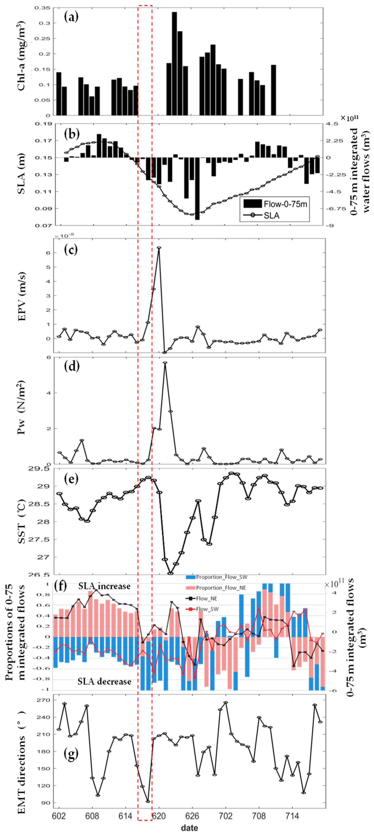
The cyclonic eddy in the study area was generated by the strong EPV during typhoon at 20 June (Figure 5c). However, the study area averaged SLA started to decrease four days before typhoon (12 June, Figure 7b). The Ekman Layer Depth (ELD) during these days (12–15 June) was 65 m in average with positive EPV (0.18 × 10⁻⁵ m/s in average) and southwestward Ekman Mass Transport (EMT, 205° in average, Figure 7g). The EMT modified the movement of seawater masses in the study area, resulting in divergence and convergence of seawater in the ELD and thus changing the vertical movement [9,29]. The 0–75 m integrated water flows (similar to the ELD) showed decreasing trend and southwestward output (−2 × 10¹¹ m3, −2.5 × 10¹¹ m3, −3.2 × 10¹¹ m3 on 13–15 June, respectively, Figure 7f) off the study area due to the southwestward EMT during these days (Figure 7b,g), and therefore causing divergences in the upper layer of the study area, especially over the pre-typhoon anti-cyclonic eddy (Figure 5b and Figure 7b,f). The SLA decreasing estimated from these southwestward EMT could reach more than 0.1 m which coincided with the maximum SLA difference shown in Figure 7b. Moreover, the SLA at where the cyclonic eddy would generate showed little changes (Figure 5c and Figure 8b). Therefore, the decrease of the area average SLA several days before the arrival of the typhoon (12 June) in the study area was mainly due to the westward EMT (Figure 7g) decreased anti-cyclonic eddy rather than the generation of the typhoon-induced cyclonic eddy (Figure 5c and Figure 8b). This westward Ekman transport probably related to the generation of the typhoon (13 June) southeast to the study area along the Philippines (Figure 1). Therefore, the cyclonic eddy in the study area was mainly induced by the typhoon and the decrease of the SLA four days before typhoon was due to the decrease of the anti-cyclonic eddy.
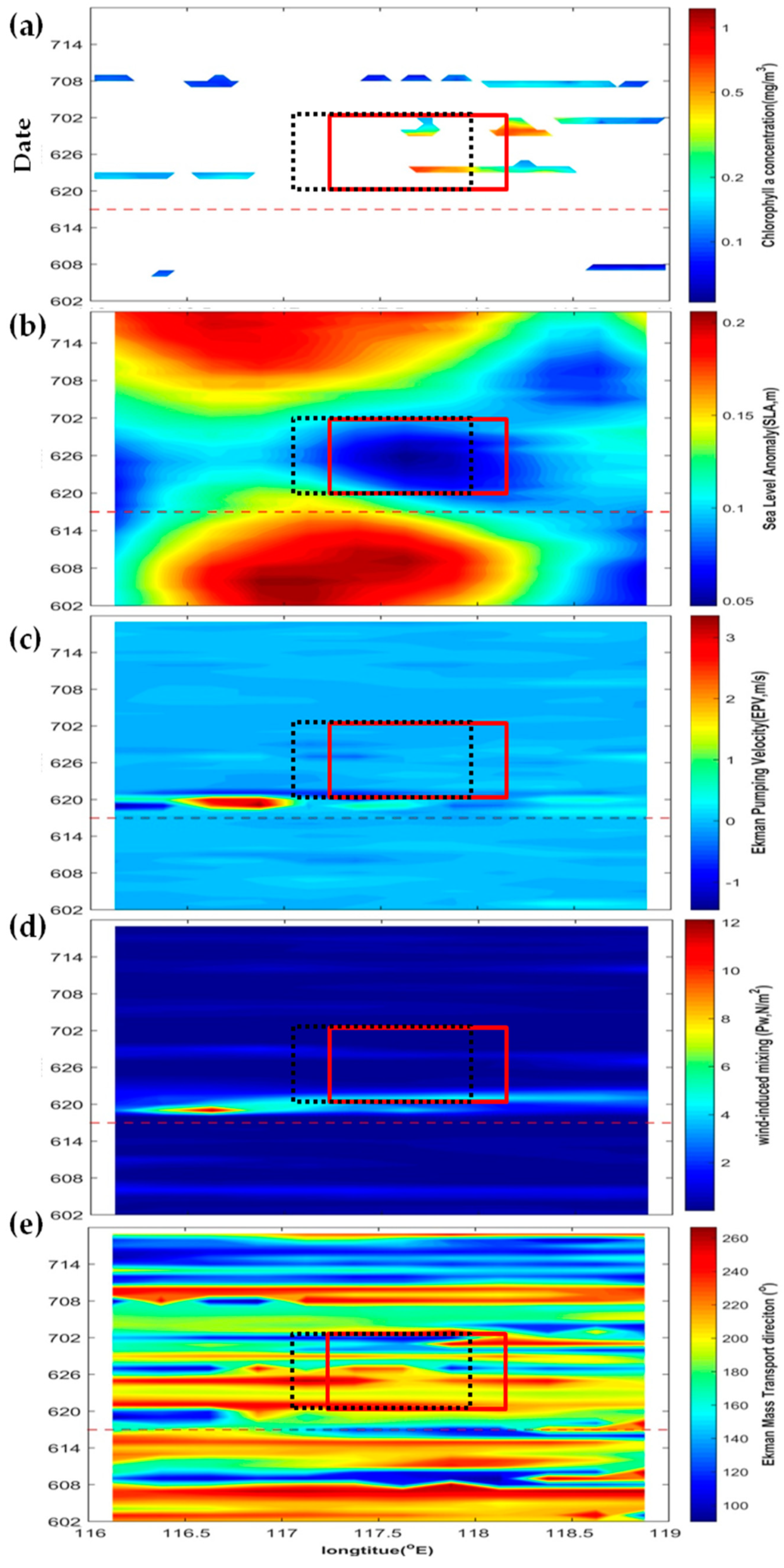
The partial correlations between Chl-a and each factor can show the importance of affecting the surface Chl-a changes [2]. Although the timeseries of the average values for each factor within the study region seems to have strong relations with the surface Chl-a one–three days after the typhoon (Figure 7), the surface Chl-a has a much stronger relationship with the SLA and SST (R = −0.62 and R = −0.73, respectively, Table 2) than the EPV, wind-stirring and rainfall (R = 0.09, R = 0.09, and R = −0.01, respectively, Table 2) after typhoon. In addition, the surface Chl-a shows weak relationship with the SLA and SST (R = −0.16 and R = 0.08, respectively) but strong relationship with the wind-stirring (R = 0.57) before typhoon. These indicated that, the typhoon-induced cyclonic eddy and SST cooling played more important roles than the wind-driven upwelling and wind-induced mixing after the typhoon, and this typhoon-induced cyclonic eddy could play one of the most important roles in the surface Chl-a increasing. These are consistent with slightly increase of the EPV (Figure 6) but significantly decrease of the SLA over the study region (Figure 4). This enhancing cyclonic eddy can generate strong upwelling through eddy-pumping and supply nutrients from deeper water for the growth of the surface phytoplankton [2,12,30]. It is also consistent with Chen’s finding that the typhoon-induced cold eddy played an important role in increasing the surface Chl-a [15]. Then, the strongest relationship between the SLA and the SST (R = 0.65) after the typhoon indicates that the typhoon-induced cyclonic eddy was mainly generated by the significant SST cooling which could cause divergence at the sea surface and overturn of the upper and deeper water [29]. In addition, a pre-existing upwelling and unstable upper ocean layer were found in 80–150 m at the center of the cyclonic eddy (Station 7, Figure 6). These upper ocean conditions then generated the enhancing cyclonic eddy 3–4 days after the typhoon at 20 June and resulted of surface Chl-a increasing through eddy-pumping upwelling [12,31]. Moreover, the spatial and temporal distribution of wind forcing and eddy effects shown in Figure 8 also clearly presents a much more similar pattern between the Chl-a and the SLA than other factors along the 18° E, where the place with increasing Chl-a coincided with the area of decreasing SLA (Figure 8a,b). Thus, the typhoon-induced cyclonic eddy (SLA) played one of the most important roles in the surface Chl-a increasing not only in temporal but also in spatial distribution rather than the EPV or the wind-stirring mixing.
4.3.2. Effect of the Ekman Transport on the Surface Chl-a after the Typhoon
Before discussing the Ekman mass transport (EMT), the common horizontal motion of Rossby wave, which causes water to meander in wide loops north and south but only move the surface of the ocean up or down a few centimeters [29,32], should be discussed. The Hovmöller graph (Figure 8b) [29,32] was made to recognize the Rossby wave before and after the typhoon. According to Figure 8b, no obvious Rossby wave signal was observed, as the pre-typhoon cyclonic eddy (low SLA) outside the study at 119° E gradually disappeared after typhoon and show less westwards connection with the post-typhoon cyclonic eddy (low SLA) in the study region at 117.8° E, and this post-typhoon cyclonic eddy (low SLA) in the study region presented a eastward transport 10 days after the Linfa which was contrary with the westward transport of the Rossby wave. Figure 5d,e also showed the eastward transport of the cyclonic eddy in the study area. In addition, the almost northward wind field lasted for more than one week in the study area, which indicated that this continuous eastward Ekman transport after typhoon should play an important role in the eastward movement of the typhoon-induced cyclonic eddy in the study area. Therefore, the typhoon-induced cyclonic eddy in the study area was not propagated from the pre-typhoon cyclonic eddy east of the study area but due to the typhoon-induced Ekman transport.
The Ekman mass transport (EMT) directions after the typhoon changed into southwestward (with the angle of ~210° from the north, Figure 7 and Figure 8), and the surface Chl-a presented a southwestward pattern according to the SLA pattern during this period (Figure 2 and Figure 4). It indicated that the distribution of the Chl-a southwest to the cyclonic eddy could be affected by the wind-induced advection transport several days after the typhoon from 20 June. It was documented that the surface Chl-a blooms over the western SCS was transported offshore through the Ekman transport [33]. Chen also found that the surface Chl-a bloom over the Hainan Island was affected by the Ekman transport and presented an offshore pattern [34]. Thus, the surface Chl-a was possible transported to the southwest of the typhoon-induced cyclonic eddy through the Ekman mass transport, which lead to phase shift between the SLA and the surface Chl-a.
4.3.3. Effect of the SST on the Surface Chl-a after the Typhoon
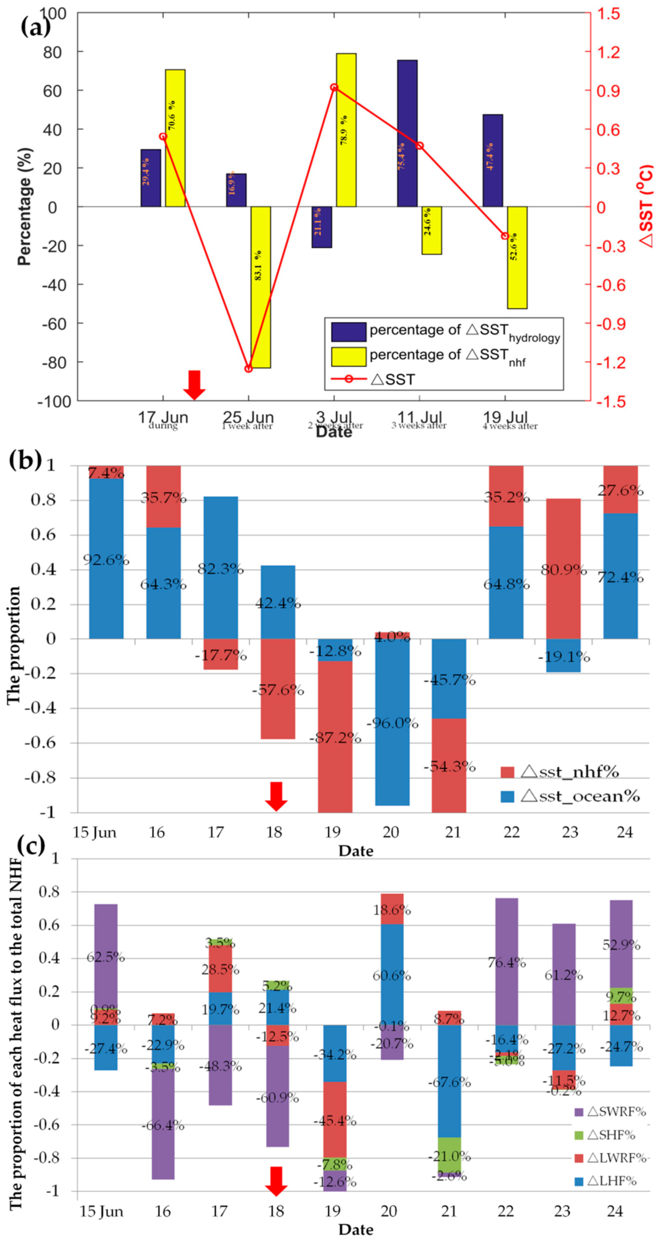
The SST (mentioned in Section 4.3.1) could play a more important role than the typhoon-induced cyclonic eddy in the surface Chl-a according to its stronger relation with the surface Chl-a comparing with the SLA (Table 2). A significant SST cooling (~2.5 °C) occurred especially at the right side of the typhoon looping area at where the surface Chl-a blooms and cyclonic eddy generated (Figure 4c). The spatial and temporal distributions of the SST match up well with that of the Chl-a (Figure 2, Figure 4, and Figure 7). The typhoon-induced SST cooling was usually right bias to the typhoon track in the Northern Hemisphere, and it would break the upper ocean stratification, lead to the overturn of surface water and deeper water, and cause upper ocean divergence and upwelling after typhoon [9,35]. The divergence and strong mixing caused by this typhoon-induced SST cooling can uplift nutrients from deeper layer to subsurface or even the surface, and therefore supply for the growth of the surface and subsurface phytoplankton [2,7,35]. In addition, the temperature of ~20–25 °C is usually phytoplankton favorable [1,36], so the typhoon-induced SST cooling especially in summer will be favored for the growth of the surface phytoplankton. The main processes for the typhoon-induced SST cooling include vertical mixing, Ekman pumping, and heat loss to the atmosphere [9,20], so quantitative analysis was made to classify the contribution of the typhoon-induced vertical motion (vertical mixing and the upwelling) and the air–sea heat exchange (net heat flux, NHF) in the SST (Figure 9). The NHF is an important indicator for measuring the exchange of air–sea heat exchange [17], and the SST change due to the NHF alone () can be estimated from Formula (3) [20].
After the typhoon Linfa, the ratios of the in the total SST changes (70.6%, 83.1%, and 78.9% during, one week after, and two weeks after the typhoon, respectively, Figure 9a) were much higher than that of the SST changes caused by the marine physical processes (29.4%, 16.9%, and 21.1% during, one week after, and two weeks after the typhoon, respectively, Figure 9a). The daily area averaged ratio of the also turned into big negative values and was much greater than that of the SST changes caused by the marine physical processes when the typhoon arrived the study area (Figure 9b). It should be noted that when the typhoon looping in the study area inducing the maximum EPV (20 June), the ocean processes accounts for more than 90% of the SST drop which coincided with previous finding [9,37]. Just after the looping of the typhoon, the EPV restored rapidly and the NHF played the major role in the SST drop again at 21 June. In addition, the latent heat flux (LHF) gradually overwhelmed the shortwave radiation flux (SWRF) and played a leading role in controlling the NHF one–three days after the typhoon, and it contributed almost 68% of the heat loss of the ocean leading to significant SST cooling 3 days after the typhoon on 21 June (Figure 9c). All these indicated that the NHF (mainly the LHF) played a leading role in the SST cooling during the typhoon except for its looping period, and this negative just after the typhoon regulated the upper ocean stratification and resulted in upper ocean vertical mixing and divergence, which then uplifted the deeper nutrients to the surface and the subsurface supplying for the growth of the surface and the subsurface phytoplankton [9,29,35,37]. Three weeks after the typhoon, the marine physical processes gradually play a major role in the (Figure 9), which indicates that the marine physical processes played the major role in affecting the sea surface Chl-a three weeks after the typhoon. As was mentioned in Section 4.3.1, the typhoon-induced cyclonic eddy (Table 2) plays the major role in increasing the surface Chl-a along with wind-stirring mixing, Ekman pumping upwelling, and the typhoon-induced cyclonic eddy. Therefore, the NHF (air–sea heat exchange) played a key role in indirectly increasing the surface Chl-a through cooling the SST, and the marine physical processes gradually gain major role in affecting the sea surface Chl-a mainly through the typhoon-induced cyclonic eddy (Table 2) three weeks after the typhoon.
4.4. Influence of Biochemical Processes on the Chl-a Variability
Physical processes increase the surface Chl-a mainly through the uplift of the subsurface high Chl-a waters and uptake of the nutrients fluxes, which fuel the growth of phytoplankton through the biochemical processes [4,38]. Upwelling of the nutrient-rich waters from the deeper layer is the principal source of nutrients fueling the phytoplankton especially over the oligotrophic ocean [1,38]. The major nutrient element limiting phytoplankton biomass throughout most of the world oceans is nitrogen [1,14]. Light is also essential for the growth of the phytoplankton [1]. In this section, we mainly focused on the effect of nitrate and light as the biochemical processes to the Chl-a during the passage of Linfa over the northwestern SCS.
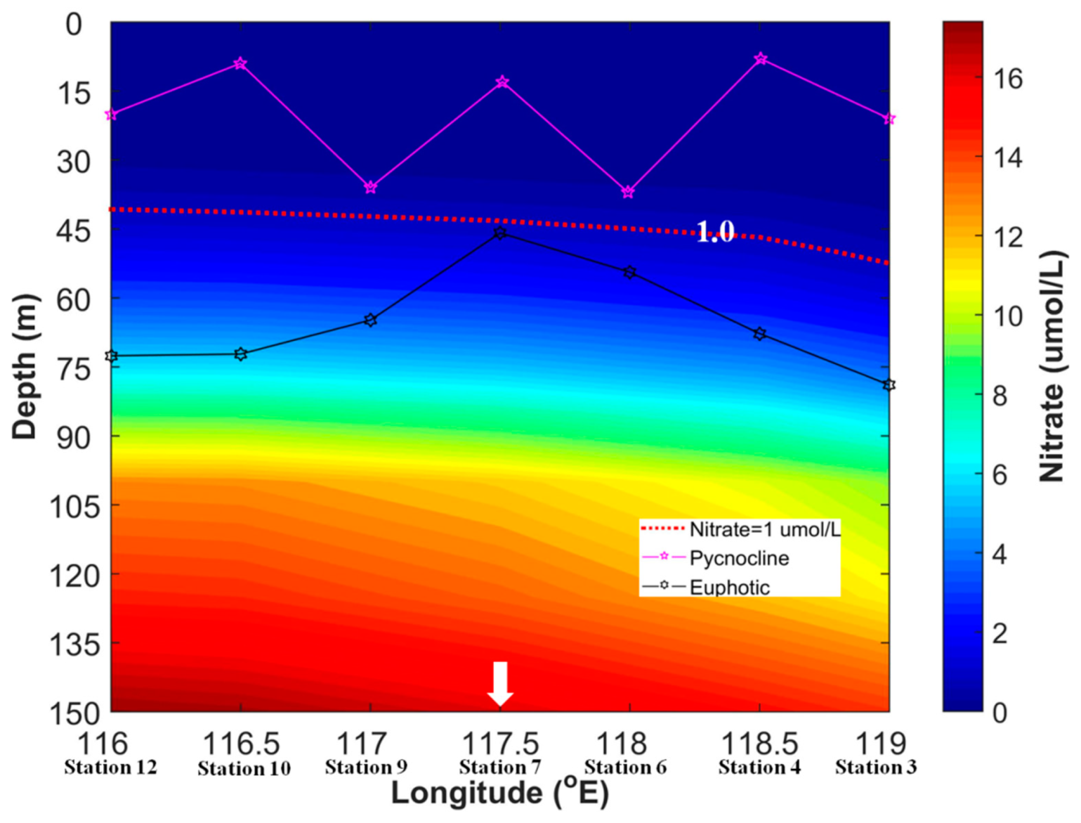
Figure 10 shows the monthly nitrate at June along the 18° N derived from the WOA13 dataset. These WOA13 monthly nutrients profiles could help us to analyze the possible vertical responses of biochemical processes (nutrients and light) and their impacts on the surface Chl-a.
The 1 μmol/L of monthly nitrate contour is deeper than the MLD along the 18°N section (Figure 10). According to Nelson’s theory [39], the nitrate = 1 μmol/L is the threshold of minimum nutrient content for phytoplankton growth. As mentioned in 4.1, the surface and euphotic-integrated Chl-a increased significantly around 117–118° E (Stations 6, 7, and 9) were mainly due to the growth of the phytoplankton. This indicated that the nutricline (nitrate = 1 μmol/L) must be uplifted to a shallower layer and the deeper waters with high nutrients should be transported to the subsurface and the surface, so that supplying adequate nutrients for the growth of phytoplankton within the euphotic layer. This uplift of the nitrate concentration is the basic and key condition for the Chl-a blooming over the oligotrophic northern South China Sea (NSCS) [4]. In addition, the euphotic depths one week after the typhoon along the 18° N were much deeper than the MLD and the climatology monthly nutricline (nitrate = 1 μmol/L) in June, and the euphotic layer depth shows a peak over Station 7 (the center of the typhoon-induced cyclonic eddy, Figure 10) leading to a closer distance between the depth of the euphotic and the climatology monthly nutricline as well as the MLD [38]. This was consistent with the eddy-pumping upwelling caused by the typhoon-induced over this Station 7 [40] and indicated that the light was not the limiting biochemical condition for the increasing surface and euphotic layer-integrated Chl-a before and after the typhoon. Therefore, among the biochemical processes, the uplift of nutrients and sufficient light contributed to the growth of surface phytoplankton and the surface Chl-a blooms over the study area in the NSCS after the typhoon.
5. Conclusions
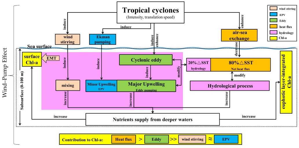
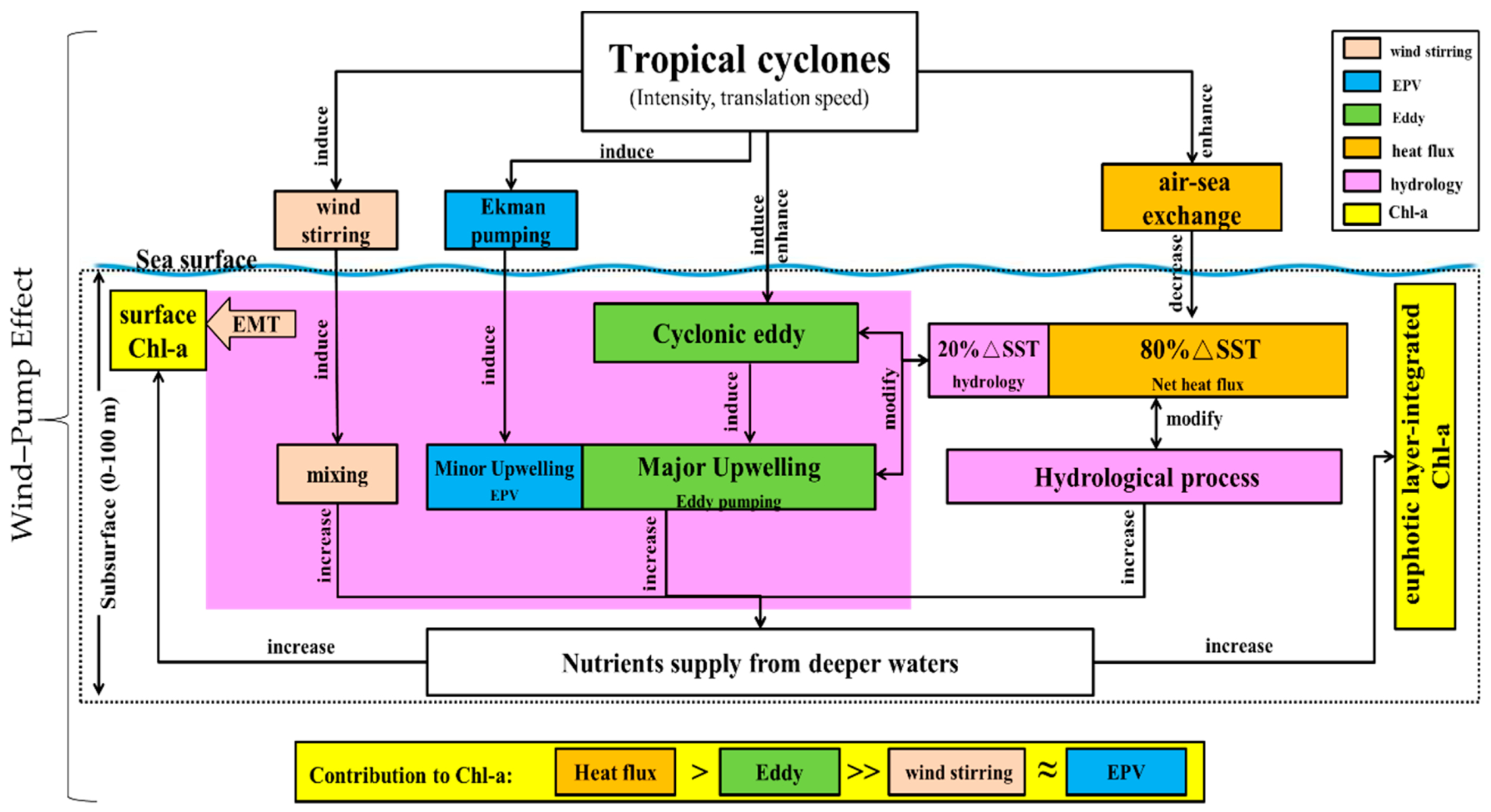
The graphical abstract (Figure 11) illustrates the Chl-a response to “Wind Pump” impact on the upper ocean conditions during the typhoon Linfa considering the air–sea exchange.
- (1)
- The growth of the surface and euphotic layer-integrated phytoplankton (Chl-a) were affected by the Chl-a entrainment in the MLD through typhoon-induced vertical mixing and entrainment, while the eddy-pumping play a much important role in the Chl-a entrainment after the typhoon;
- (2)
- The eddy-pumping caused by the typhoon-induced cyclonic eddy played the major role in the surface Chl-a increasing rather than other upper ocean physical processes (such as the EPV, the wind-stirring mixing, and the Rossby wave) after typhoon;
- (3)
- The spatial shift between the surface Chl-a and the typhoon-induced cyclonic eddy should be due to the Ekman transport, and the movement of the cyclonic eddy was mainly due to the typhoon wind stress rather than the Rossby wave;
- (4)
- The Net Heat Flux (air–sea exchange) played a key role in indirectly increasing the surface Chl-a rather than the marine physical processes through cooling the SST until two weeks after the typhoon;
- (5)
- Nutrient (nitrate) uplifting, rather than light, was the main biochemical factor restricting the growth of surface and euphotic-integrated phytoplankton over the study area in the NSCS after the typhoon Linfa.
Author Contributions
Y.L. and D.T. jointly conducted the research, data collecting, processing, analysis, and manuscript writing. Y.L. worked on the quantification model and images preparation; D.T. designed and advised the research project and provided project support; M.E. assisted data analysis and paper editing.
Funding
The research was funded by the National Natural Science Foundation of China (41430968, 41876136), the 21st Century Maritime Silk Road Collaborative Innovation Center Marine Environmental Science Project (2015HS05), and the Guangdong Provincial Science and Technology Department Project (2017B030301005).
Acknowledgments
Authors thank the “National Science and Technology Basic Condition Platform-National Earth System Science Data Sharing Service Platform-Nanhai and its adjacent sea area scientific data center (http://ocean.geodata.cn)” for providing data support. Thanks to the LORS of the Guangdong Provincial Key Laboratory of Ocean Remote Sensing and the National Key Laboratory of Tropical Marine Environment LTO for their support. Thanks to Wendi Zheng, Pro. Jinyu Sheng, Huibin Xing, Wenzhao Liang and the team members for their help.
Conflicts of Interest
The authors declare no conflict of interest.
References
- Falkowski, P.G. The role of phytoplankton photosynthesis in global biogeochemical cycles. Photosynth. Res. 1994, 39, 235–258. [Google Scholar] [CrossRef] [PubMed] [Green Version]
- Zhao, H.; Wang, Y.Q. Phytoplankton increases induced by tropical cyclones in the South China Sea during 1998–2015. J. Geophys. Res. 2018, 123. [Google Scholar] [CrossRef]
- Hallegraeff, G.M. A review of harmful algal blooms and their apparent global increase. Phycologia 1993, 32, 79–99. [Google Scholar] [CrossRef] [Green Version]
- Pan, G.; Chai, F.; Tang, D.L.; Wang, D.X. Marine phytoplankton biomass responses to typhoon events in the South China Sea based on physical-biogeochemical model. Ecol. Model. 2017, 356, 38–47. [Google Scholar] [CrossRef]
- Lin, I.; Liu, W.T.; Wu, C.C.; Wong, G.T.F.; Hu, C.M.; Chen, Z.Q.; Liang, W.D.; Yang, Y.; Liu, K.K. New evidence for enhanced ocean primary production triggered by tropical cyclone. Geophys. Res. Lett. 2003, 30. [Google Scholar] [CrossRef] [Green Version]
- Babin, S.M.; Carton, J.A.; Dickey, T.D.; Wiggert, J.D. Satellite evidence of hurricane-induced phytoplankton blooms in an oceanic desert. J. Geophys. Res. 2004, 109. [Google Scholar] [CrossRef]
- Ye, H.J.; Sui, Y.; Tang, D.L.; Afanasyev, Y.D. A subsurface chlorophyll a bloom induced by typhoon in the South China Sea. J. Mar. Syst. 2013, 128, 138–145. [Google Scholar] [CrossRef]
- Lin, J.R.; Tang, D.L.; Alpers, W.; Wang, S.F. Response of dissolved oxygen and related marine ecological parameters to a tropical cyclone in the South China Sea. Adv. Space Res. 2014, 53, 1081–1091. [Google Scholar] [CrossRef]
- Price, J.F. Upper ocean response to a hurricane. J. Phys. Oceanogr. 1981, 11, 153–175. [Google Scholar] [CrossRef]
- Sun, Q.Y.; Tang, D.L.; Legendre, L.; Shi, P. Enhanced sea-air CO2 exchange influenced by a tropical depression in the South China Sea. J. Geophys. Res. 2015, 119, 6792–6804. [Google Scholar] [CrossRef]
- Zhao, H.; Han, G.Q.; Zhang, S.W.; Wang, D.X. Two phytoplankton blooms near Luzon Strait generated by lingering Typhoon Parma. J. Geophys. Res. 2013, 118, 412–421. [Google Scholar] [CrossRef]
- He, Q.Y.; Zhan, H.G.; Cai, S.Q.; Li, Z.M. Eddy effects on surface chlorophyll in the northern South China Sea: Mechanism investigation and temporal variability analysis. Deep-Sea Res. Part I 2016, 112, 25–36. [Google Scholar] [CrossRef]
- Liang, W.Z.; Tang, D.L.; Luo, X. Phytoplankton size structure in the western South China Sea under the influence of a ‘jet-eddy system’. J. Mar. Syst. 2018, 187, 82–95. [Google Scholar] [CrossRef]
- Dugdale, R.C. Nutrient limitation in sea - dynamics identification and significance. Limnol. Oceanogr. 1967, 12, 685–695. [Google Scholar] [CrossRef]
- Chen, Y.Q.; Tang, D.L. Eddy-feature phytoplankton bloom induced by a tropical cyclone in the South China Sea. Int. J. Remote Sens. 2012, 33, 7444–7457. [Google Scholar] [CrossRef]
- Wu, L.G.; Wang, B.; Braun, S.A. Impacts of Air-Sea Interaction on Tropical Cyclone Track and Intensity. Mon. Weather Rev. 2004, 133, 3299–3314. [Google Scholar] [CrossRef]
- Liu, S.S.; Zhang, L.F.; Zhang, X.H. Characteristics analysis on rapid intensification of typhoon Mujigae (1522) over the offshore area of China. J. Meteor. Sci. 2017. [Google Scholar] [CrossRef]
- Shay, L.K.; Elsberry, R.L.; Black, P.G. Vertical structure of the ocean current response to a hurricane. J. Phys. Oceanogr. 1989, 19, 649–669. [Google Scholar] [CrossRef]
- Pan, J.Y.; Huang, L.; Devlin, A.T.; Lin, H. Quantification of typhoon-induced phytoplankton blooms using satellite multi-sensor data. Remote Sens. 2018, 10, 318. [Google Scholar] [CrossRef]
- Ye, H.J.; Sheng, J.Y.; Tang, D.L.; Siswanto, E.; Kalhoro, M.A.; Sui, Y. Storm-induced changes in pCO2 at the sea surface over the northern South China Sea during Typhoon Wutip. J. Geophys. Res. 2017, 122, 4761–4778. [Google Scholar] [CrossRef]
- Wijesekera, H.W.; Gregg, M.C. Surface layer response to weak winds, westerly bursts, and rain squalls in the western Pacific Warm Pool. J. Geophys. Res. 1996, 101, 977–997. [Google Scholar] [CrossRef]
- Cao, W.X.; Yang, Y.Z. A bio-optical model for ocean photosynthetic available radiation. J. Trop. Oceanogr. 2002, 21, 47–54. [Google Scholar]
- Uitz, J.; Claustre, H.; Morel, A.; Hooker, S.B. Vertical distribution of phytoplankton communities in open ocean: An assessment based on surface chlorophyll. J. Geophys. Res. 2006, 111. [Google Scholar] [CrossRef]
- Lin, I.I. Typhoon-induced phytoplankton blooms and primary productivity increase in the western North Pacific subtropical ocean. J. Geophys. Res. 2012, 117. [Google Scholar] [CrossRef]
- Liu, Z.L.; Chen, Z.Y.; Zhou, B.F.; Zhang, T.; Ding, T. The seasonal distribution of the standing stock of phytoplankton in the source area of the kuroshio and adjacent areas. Tran. Oceanol. Limnol. 2006, 58–63. [Google Scholar] [CrossRef]
- Shay, L.K.; Goni, G.J.; Black, P.G. Effects of a warm oceanic feature on hurricane Opal. Mon. Weather Rev. 2000, 128, 1366–1383. [Google Scholar] [CrossRef]
- Zhang, H.; Chen, D.K.; Zhou, L.; Liu, X.H.; Ding, T.; Zhou, B.F. Upper ocean response to typhoon Kalmaegi (2014). J. Geophys. Res. 2016, 121, 6520–6535. [Google Scholar] [CrossRef]
- Huang, L.; Zhao, H.; Pan, J.Y.; Devlin, A. Remote sensing observations of phytoplankton increases triggered by successive typhoons. Front. Earth Sci. 2017, 11, 601–608. [Google Scholar] [CrossRef]
- Talley, L.D.; Pickard, G.L.; Emery, W.J.; Swift, J.H. Chapter 5–Mass, Salt, and Heat Budgets and Wind Forcing. In Descriptive Physical Oceanography: An Introduction; Academic Press: Cambridge, MA, USA, 2011. [Google Scholar]
- Liu, F.F.; Tang, S.L. Influence of the interaction between typhoons and oceanic mesoscale eddies on phytoplankton blooms. J. Geophys. Res. 2018, 123, 2785–2794. [Google Scholar] [CrossRef]
- Gaube, P.; Chelton, D.B.; Strutton, P.G.; Behrenfeld, M.J. Satellite observations of chlorophyll, phytoplankton biomass, and Ekman pumping in nonlinear mesoscale eddies. J. Geophys. Res. 2013, 118, 6349–6370. [Google Scholar] [CrossRef] [Green Version]
- Jin, X.; Kwon, Y.-O.; Ummenhofer, C.C.; Seo, H.; Schwarzkopf, F.U.; Biastoch, A.; Boening, C.W.; Wright, J.S. Influences of Pacific Climate Variability on Decadal Subsurface Ocean Heat Content Variations in the Indian Ocean. J. Clim. 2018, 31, 4157–4174. [Google Scholar] [CrossRef]
- Wang, J.J.; Tang, D.L.; Sui, Y. Winter phytoplankton bloom induced by subsurface upwelling and mixed layer entrainment southwest of Luzon Strait. J. Mar. Syst. 2010, 83, 141–149. [Google Scholar] [CrossRef]
- Chen, Y.Q.; Tang, D.L. Remote sensing analysis of impact of typhoon on environment in the sea area south of Hainan Island. Procedia Environ. Sci. 2011, 10, 1621–1629. [Google Scholar] [CrossRef]
- Fu, D.Y.; Pan, D.L.; Mao, Z.H.; Ding, Y.Z.; Chen, J.Y. The effects of chlorophyll-a and SST in the South China Sea area by typhoon near last decade. SPIE Remote Sens. 2009. [Google Scholar] [CrossRef]
- Chin, T.G.; Chen, C.F.; Liu, C.S.; Wu, S.S. Influence of temperature and salinity on the growth of three species of planktonic diatoms. Oceanol. Limnol. Sin. 1965, 7, 373. [Google Scholar]
- Veeranjaneyulu, C.; Deo, A.A. Study of upper ocean parameters during passage of tropical cyclones over Indian seas. Int. J. Remote Sens. 2019, 40, 4683–4723. [Google Scholar] [CrossRef]
- Son, S.; Platt, T.; Fuentes-Yaco, C.; Bouman, H.; Devred, E.; Wu, Y.; Sathyendranath, S. Possible biogeochemical response to the passage of Hurricane Fabian observed by satellites. J. Plankton Res. 2007, 29, 687–697. [Google Scholar] [CrossRef] [Green Version]
- Liu, C.; Kang, J.C.; Wang, G.D.; Zhu, W.W.; Sun, W.Z.; Li, Y. Monthly spatial variation of nutrients and nutrient limitation in kuroshio of East China Sea. Resour. Sci. 2012, 34, 1375–1381. [Google Scholar]
- Xu, H.B.; Tang, D.L.; Liu, Y.P.; Li, Y. Dissolved oxygen responses to tropical cyclones" Wind Pump" on pre-existing cyclonic and anticyclonic eddies in the Bay of Bengal. Mar. Pollut. Bull. 2019, 146, 838–847. [Google Scholar] [CrossRef]
Figure 1.
Map of the study area and typhoon path (the blue box represents the study area; black line means the path of typhoon; the green, yellow, and red dots represent the tropical depression (td), tropical storm (ts), and typhoon (tp), respectively; the pink points and pink numbers represent the station positions and station names).

Figure 2.
Map of the changes of the Chl-a before and after the typhoon Linfa. (a) One week before typhoon; (b) during typhoon; (c) one week after typhoon; (d) two weeks after typhoon; (e) time series of the area average surface Chl-a within study area shown as the red box.
Figure 2.
Map of the changes of the Chl-a before and after the typhoon Linfa. (a) One week before typhoon; (b) during typhoon; (c) one week after typhoon; (d) two weeks after typhoon; (e) time series of the area average surface Chl-a within study area shown as the red box.

Figure 3.
Spatial distribution map of rainfall, sea surface temperature (SST), and sea level height anomaly (SLA) with sea surface geostrophic currents (geo-SSCs) before and after the typhoon (first column: Rainfall (mm); second column: Sea surface temperature (SST, °C); third column: SLA (cm) with geo-SSCs (m/s); (a–d) represent 1 week before, during, 1 week after, and 2 weeks after the typhoon Linfa; the blue box indicates the study area; the dotted line indicates the typhoon path).

Figure 4.
Distribution map of the Ekman pumping velocities (EPV, m/s) and wind fields before and after the typhoon (a) one week before typhoon; (b) during typhoon; (c) one week after typhoon; (d) two weeks after typhoon; the blue box indicates the study area, the black dotted line indicates the typhoon path, and the arrows indicate the wind vectors).

Figure 5.
Daily distribution map of the Chl-a (mg/m3), EPV (m/s), and SLA with geo-SSCs before and after the typhoon ((a) 10 days before typhoon; (b) during typhoon; (c) just after typhoon; (d) 3 days after typhoon; (e) 2 weeks after the typhoon; the blue box indicates the study area, the black dotted line indicates the typhoon path, and the arrows in the second column indicate the wind vectors, the arrows in the third column indicate the geo-SSCs).

Figure 6.
Hydrological profiles of the 18° N from cruise data in 16–17 July, 2009. [(a) Temperature profiles (°C); (b) salinity profiles (psu); (c) density profiles (kg/m3); the black dash line box represents the study region; the black line with dots represents the MLD; the white arrow shows the position of the maximum surface Chl-a], and the graph of the potential temperature, salinity, and potential density from cruise data [S,T,D represent the potential temperature, salinity, and potential density, respectively. (d1) Profiles during (Station 6 at 18° N, 119° E) the typhoon; (d2) Profiles after (Station 20) the typhoon. (e1) Temperature, Salinity and (e2) Density profiles of 4 stations within the study area one day before (Station 9) and during (Stations 4, 6, and 7) the typhoon].

Figure 7.
Time series of area average values about each factor within the study region before and after the typhoon. (a) Chl-a (mg/m3); (b) SLA (m) and 0–75 m integrated water flows minus that of 2 June (m3); (c) EPV (m/s); (d) Pw (N/m2); (e) SST (°C); (f) proportions and values of 0–75 m integrated water flows minus that of 2 June (m3, red and black lines represent the values of southwestward and northeastward water masses transport, respectively; the blue and red bars represent the proportions of southwestward and northeastward water masses transport, respectively; positive means inflows and divergence); red dash line box represents the period of typhoon passing the study region.

Figure 8.
Horizontal time section of each parameter in the study area before and after the typhoon. (a) Chl-a (mg/m3); (b) SLA (m); (c) EPV (m/s); (d) Pw (N/m2); (e) direction of the EMT (°); red dashed line represents the passage of the typhoon, the black dashed line box represents the position of the surface Chl-a blooms one week after the typhoon, the red box represents the position of the cyclonic eddy one week after the typhoon.

Figure 9.
Study area averaged heat budget analysis to the changes of the sea surface temperature (△SST) before and after the typhoon. (a) The weekly area average △SST due to net heat flux (NHF) and the ocean processes. (b) The daily area average △SST due to NHF and the ocean processes. (c) The proportion of the daily area average heat flux differences (sensible heat flux (SHF), latent heat flux (LHF), longwave radiation flux (LWRF), and shortwave radiation flux (SWRF)) to the total daily area averaged NHF. The red arrows represented the passing time of the typhoon Linfa. Positive values mean increase of the SST and negative values mean decrease of the SST.

Figure 10.
Monthly average nitrate distribution profile of WOA13 in June (μmol/L, the pink line with dots represents the MLD 1–2 days after the typhoon, the red dotted line represents the 1 μmol/L of nitrate contour, the black line with dots represent the euphotic depth one week after the typhoon, the white arrow represents the center of the typhoon-induced cyclonic eddy).

Figure 11.
Graphical abstract illustrates the Chl-a response to the typhoon “Wind Pump” impacts on upper ocean conditions and air–sea exchange. The EMT represents the Ekman mass transport, the EPV represents the Ekman pumping velocity, the black dashed line box represents the subsurface water from 0–100 m, the blue wavy line indicates the sea surface, and different colors represent different processes shown in the northeastern legend. The importance ranking of the roles in the Chl-a increasing is shown at the bottom of this figure within the yellow box.


Table 1.
The surface and column-integrated Chlorophyll a concentration, the MLD, the euphotic layer depth (ELD), and the Chl-a entrainment before and after the typhoon.
Table 1.
The surface and column-integrated Chlorophyll a concentration, the MLD, the euphotic layer depth (ELD), and the Chl-a entrainment before and after the typhoon.
| Areas | Recording Periods of the Typhoon | Surface Chl-a (mg/m3) | Euphotic Layer-Integrated Chl-a (mg/m2) | MLD(m) | Euphotic Layer depth (m) | Chl-a Entrainment (mg/m3) |
|---|---|---|---|---|---|---|
| Study area average | −1 week | 0.08 | 10.90 | 8.0 | 84.7 | 0.13 |
| 1 week | 0.21 | 18.33 | 9.3 | 60.4 | 0.30 | |
| 2 weeks | 0.14 | 14.86 | 5.0 | 69.7 | 0.21 | |
| Eddy center (Station 7) | −1 week | 0.08 | 10.64 | 7.3 | 84.7 | 0.13 |
| 1 week | 0.46 | 27.79 | 8.7 | 45.9 | 0.61 | |
| 2 weeks | 0.12 | 13.57 | 5.0 | 60.4 | 0.22 |
Table 2.
The partial correlation between time series of the area average Chl-a, SLA, EPV, wind-stirring (Pw), SST, rainfall, and Ekman Mass Transport (EMT) directions over the study area.
Table 2.
The partial correlation between time series of the area average Chl-a, SLA, EPV, wind-stirring (Pw), SST, rainfall, and Ekman Mass Transport (EMT) directions over the study area.
| Period | Factors | Chl-a | SLA | EPV | Pw | SST | rain | EMT_dir |
|---|---|---|---|---|---|---|---|---|
| Partial correlation (R) before typhoon (2–15 June) | Chl-a | 1.00 | −0.16 | 0.23 | 0.57 | 0.08 | 0.23 | −0.07 |
| SLA | - | 1.00 | 0.04 | −0.02 | −0.72 | 0.13 | 0.07 | |
| EPV | - | - | 1.00 | 0.35 | −0.34 | 0.16 | −0.04 | |
| Pw | - | - | - | 1.00 | −0.37 | 0.03 | −0.05 | |
| SST | - | - | - | - | 1.00 | −0.41 | −0.02 | |
| rain | - | - | - | - | - | 1.00 | −0.48 | |
| EMT_dir | - | - | - | - | - | - | 1.00 | |
| Partial correlation (R) after typhoon (16 June–19 July) | Chl-a | 1.00 | −0.62 | 0.09 | 0.09 | −0.73 | −0.01 | −0.39 |
| SLA | - | 1.00 | −0.12 | −0.18 | 0.65 | −0.06 | 0.40 | |
| EPV | - | - | 1.00 | −0.41 | 0.14 | −0.48 | 0.30 | |
| Pw | - | - | - | 1.00 | −0.60 | 0.96 | −0.31 | |
| SST | - | - | - | - | 1.00 | −0.48 | 0.55 | |
| rain | - | - | - | - | - | 1.00 | −0.27 | |
| EMT_dir | - | - | - | - | - | - | 1.00 |
© 2019 by the authors. Licensee MDPI, Basel, Switzerland. This article is an open access article distributed under the terms and conditions of the Creative Commons Attribution (CC BY) license (http://creativecommons.org/licenses/by/4.0/).
Share and Cite
MDPI and ACS Style
Liu, Y.; Tang, D.; Evgeny, M. Chlorophyll Concentration Response to the Typhoon Wind-Pump Induced Upper Ocean Processes Considering Air–Sea Heat Exchange. Remote Sens. 2019, 11, 1825. https://0-doi-org.brum.beds.ac.uk/10.3390/rs11151825
AMA Style
Liu Y, Tang D, Evgeny M. Chlorophyll Concentration Response to the Typhoon Wind-Pump Induced Upper Ocean Processes Considering Air–Sea Heat Exchange. Remote Sensing. 2019; 11(15):1825. https://0-doi-org.brum.beds.ac.uk/10.3390/rs11151825
Chicago/Turabian StyleLiu, Yupeng, Danling Tang, and Morozov Evgeny. 2019. "Chlorophyll Concentration Response to the Typhoon Wind-Pump Induced Upper Ocean Processes Considering Air–Sea Heat Exchange" Remote Sensing 11, no. 15: 1825. https://0-doi-org.brum.beds.ac.uk/10.3390/rs11151825
Note that from the first issue of 2016, this journal uses article numbers instead of page numbers. See further details here.