Ocean Optical Profiling in South China Sea Using Airborne LiDAR


State Key Laboratory of Satellite Ocean Environment Dynamics, Second Institute of Oceanography, Ministry of Natural Resources, 36 Bochubeilu, Hangzhou 310012, China
*
Author to whom correspondence should be addressed.
Remote Sens. 2019, 11(15), 1826; https://0-doi-org.brum.beds.ac.uk/10.3390/rs11151826
Submission received: 25 June 2019
/
Revised: 28 July 2019
/
Accepted: 1 August 2019
/
Published: 5 August 2019
(This article belongs to the Section Ocean Remote Sensing)
Abstract
:Increasingly, LiDAR has more and more applications. However, so far, there are no relevant publications on using airborne LiDAR for ocean optical profiling in the South China Sea (SCS). The applicability of airborne LiDAR for optical profiling in the SCS will be presented. A total of four airborne LiDAR flight experiments were conducted over autumn 2017 and spring 2018 in the SCS. A hybrid retrieval method will be presented here, which incorporates a Klett method to obtain LiDAR attenuation coefficient and a perturbation retrieval method for a volume scattering function at 180°. The correlation coefficient between the LiDAR-derived results and the traditional measurements was 0.7. The mean absolute relative error (MAE) and the normalized root mean square deviation (NRMSD) between the two are both between 10% and 12%. Subsequently, the vertical structure of the LiDAR-retrieved attenuation and backscattering along airborne LiDAR flight tracks was mapped. In addition to this, ocean subsurface phytoplankton layers were detected between 10 to 20 m depths along the flight track in Sanya Bay. Primary results demonstrated that our airborne LiDAR has an independent ability to survey and characterize ocean optical structure.
1. Introduction
For decades, satellite ocean color remote sensing has expanded and refined our knowledge of global phytoplankton ecosystems, the ocean carbon cycle, and the ocean’s role in climate change. However, passive remote sensing has inherent limitations to resolve water vertical structure [1]. LiDAR remote sensing has the advantage of range-resolved and deeper penetration, hence providing vertical structure information, which could provide a good supplement to passive remote sensing [2]. Increasingly, LiDAR has more and more applications, including bathymetric survey [3,4] and optical profiling of water columns [5,6,7,8], also for detecting plankton scattering layers [9,10,11], bubbles [12], internal waves [13], schools of fish [14,15], and so on. However, there are no publications on using airborne LiDAR to estimate the optical property profiles in the South China Sea (SCS) so far.
Application of LiDAR technique generally requires an inversion technique to infer two quantities, attenuation and backscatter, from a single measurement [16]. One method is to separate molecules and Mie scatter using the High-Spectral-Resolution LiDAR (HSRL) technique. In the ocean, Brillouin scattered light by molecules is Doppler-shifted away from the central wavelength by about 7.7 GHz because of the speed of sound in seawater [17]. However, HSRL systems are often complex and expensive. Another approach is to assume that the ratio of LiDAR extinction-to-backscatter is known [18]. The slope method [19] is often used in homogenous mediums, while the Fernald [20] and Klett [21] methods have been widely used in inhomogeneous mediums. All these methods need the LiDAR ratio, which is very difficult to accurately obtain, especially in the sea with such a complex environment. Furthermore, the above-mentioned methods were all used for the atmosphere in the past. A theoretical development suggests that this might be a useful technique for the ocean, but actual data showed a lot of variability [22].
In this study, the applicability of airborne LiDAR for optical profiling in SCS will be presented. First, the LiDAR system design is described in Section 2.1, followed by LiDAR flight experiments and simultaneous shipborne measurements in Section 2.2. A hybrid method developed to obtain the extinction and backscattering profile is introduced in Section 2.3. A validation method for LiDAR inversion is described in Section 2.4. The result of each procedure of the hybrid method, applied to a raw LiDAR signal, is described in Section 3.1, followed by validation results for LiDAR inversion using ground-truth measurements in Section 3.2. The vertical structure distribution of LiDAR-estimated optical properties along airborne LiDAR flight tracks is mapped in Section 3.3. Finally, we compared LiDAR and traditional shipborne observations, and discuss the effects of LiDAR observation geometry on inversion in Section 4.
2. Materials and Methods
2.1. LiDAR System Design
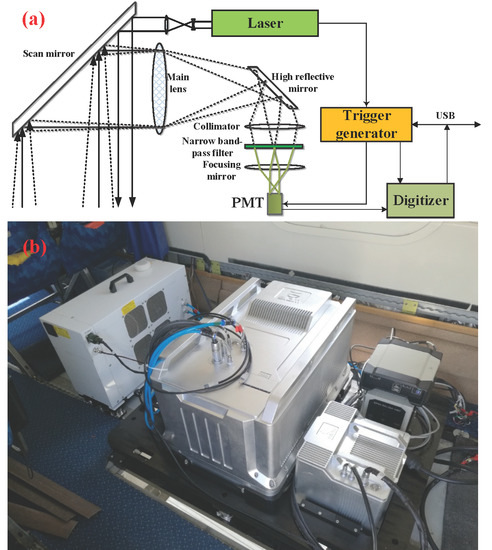
The airborne LiDAR system (AOL-SIOM) was developed by the Shanghai Institute of Optics and Fine Mechanics (SIOM). It employs a pulsed Nd:YAG laser with a 1.5 mJ pulse energy and pulse repetition frequency (PRF) of 1 kHz. The pulse width is 1.5 ns. The receiver uses a 200 mm diameter telescope with a 6 mrad field of view (FOV). A custom-built trigger generator using a Xilinx (San Jose, CA, USA) Kintex-7 field-programmable gate array (FPGA) allows a USB-programmable variable delay to gate the photomultiplier tube (PMT) and trigger the digitizers. The maximum sampling rate of the digitizer is 1.25 Giga-samples per second (GSPS); hence, the sample-rate limited depth resolution in water is 8.8 cm. Detailed technical parameters of the system has been described in previous publications [10,23], and the diagram of the major optoelectronic components and a picture of the LiDAR are shown in Figure 1.
2.2. LiDAR Flight Experiments
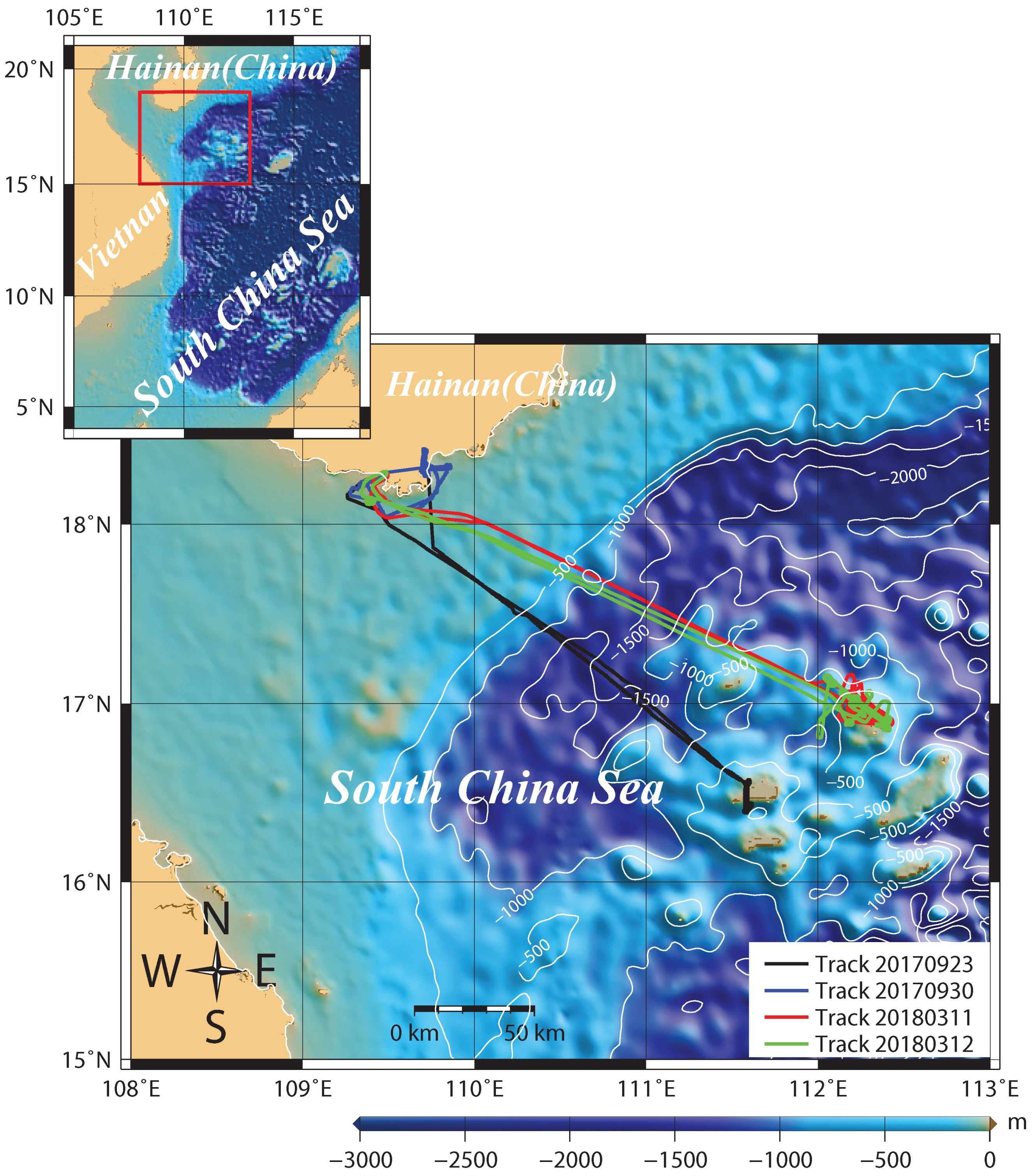
A total of four airborne LiDAR flight experiments were conducted over autumn 2017 and spring 2018 above the SCS to investigate the applicability of airborne LiDAR to obtain water optical property profiles. The LiDAR flight experiments took place on 23 and 30 September, 2017, and 11 and 12 March, 2018, respectively. The flights were made at an altitude of about 320–350 m above the water surface and a speed of 126 knots per hour. Simultaneously, shipboard measurements of water absorption and attenuation coefficients, and chlorophyll-a concentration were carried out using a profile chlorophyll fluorescent probe (RBR XR-420, RBR Ltd., Ottawa, ON, Canada) and underwater hyper spectral absorption and attenuation meter (AC-S, Wetlab Ltd., San Diego, CA, USA) along the fight tracks. AC-S is a hyperspectral instrument, produced by WET Labs in the United States, that can simultaneously measure the attenuation and absorption coefficient. The instrument provides a spectral resolution of 4 nm and a spectral measurement range of 400–720 nm. The instrument uses a dual-path combination of two argon-filled incandescent bulbs and a rotating sweep of a linearly variable filter to obtain the dispersive spectrum. The fluorometer (XR-420) from RBR Canada is a self-contained underwater device for measuring fluorescence (or chlorophyll) concentrations in water. This product has high precision and small volume, and can be used for marine environment monitoring, ecological investigation, port/river and lake water quality investigation and water quality monitoring. Its length is 200 mm and the diameter is 64 mm. The excited wavelength is 470 nm and the emission wavelength is 685 nm for a chlorophyll-a measurement with 30 nm full width at half maximum (FWHM). The sampling and measurement principles and methods used here in this study are mainly based on the Ocean Optics Protocols for the Satellite Ocean Color Sensor Validation from NASA [24]. Figure 2 shows the four flight tracks during different cruise times (color lines).
2.3. LiDAR Inversion Method
For a backscatter LiDAR system, the quasi-single-scattering LiDAR equation is:
where P(z) is the power received from range z; K is the LiDAR system constant, which means the multifactor function of instrument parameters, such as the laser energy, the optical efficiency of the receiver, and the detector electronic gain, among others [1]; β and α are the volume scattering functions, at the LiDAR scattering angle of 180°and the LiDAR attenuation coefficient, respectively. H is the equivalent altitude due to LiDAR tilt angle θ and water refractive index is n.
H can be calculated by using the LiDAR true flight height and tilt angle [25]:
where H0 is the true altitude of the airborne LiDAR, and θa is LiDAR tilt angle. The tilt angle in the water θw can be expressed by using the Snell’s law: .
The range corrected LiDAR return is logarithmically transformed:
It can be rewritten in the following differential form:
A solution to this equation requires assuming or knowing the relationship between α and β whenever . On the other hand, when the water is optically homogeneous, so that , then α could be simplified and expressed in terms to the attenuation signal slope [21]:
For inhomogeneous water, we can obtain α based on the Klett method as:
where k is the exponent according to a power law of the form , which depends on the LiDAR wavelength and various properties of the water on the interval . In this study, we assume k = 1.0.
Finally, α can be estimated as the following form:
where m means the reference boundary depth, which can be obtained from the slope method.
To obtain β, we used the perturbation retrieval (PR) method [16], which assumes that the optical parameters can be expressed as the sum of a non-varying part (that does not vary with depth) and a varying part, so that:
where S0 and β0 are the non-varying parts, which could be calculated by using a linear regression to the logarithm of the signal S for each profile:
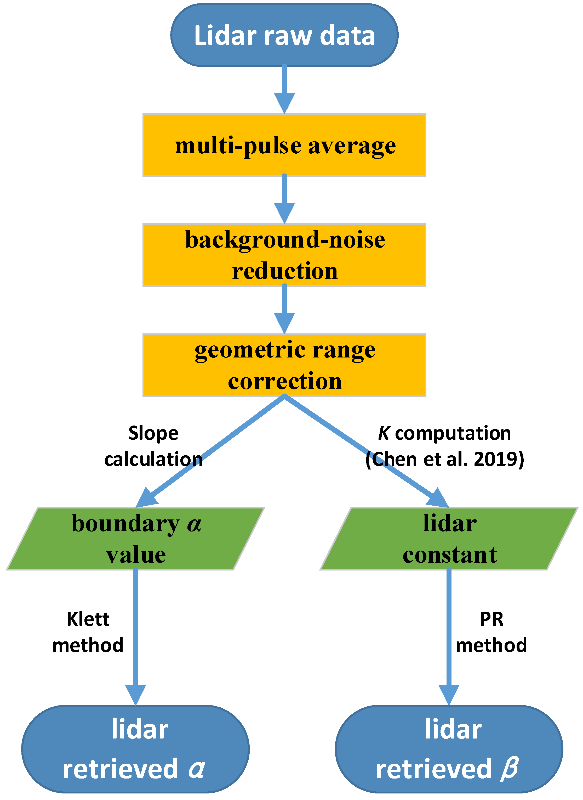
Generally, we can divide the LiDAR inversion process into six steps, as shown in Figure 3.
Step 1: Multi-pulse average and de-noising pretreatment. This method can improve the signal-to-noise ratio. Here, we average each every fifty signals and subtract the ambient noise light, which is calculated by the average of the last 200 samples of the signal.
Step 2: LiDAR geometric range correction to remove the effect of the airplane flying height.
Step 3: Obtain the initial boundary α value using the slope method (Equation (5)). The beginning 18 bins of the signal were eliminated in order to reduce the effects from the water surface reflection.
Step 4: Compute the LiDAR constant via a bio-optical calibration method [26].
Step 5: Compute the LiDAR-retrieved α and β based on a hybrid method which incorporates the Klett method and the PR method (Equations (7) and (8)). In addition, we could obtain the particle backscattering bbp and the other parameters though some bio-optical models, for instance, [27].
Step 6: Process each profile one by one and draw all the profiles along the flight tracks.
2.4. Evaluation Method
The accuracy of LiDAR-retrieved α and β may be estimated by two statistical indices: the systematic error (bias) and the random error. Here, we use the mean absolute relative error (MAE) and Root Mean Square Deviation (NRMSD) to determine the systematic and random errors, respectively. These metrics are defined as follows:
where Rlidar and Rm are the LiDAR-retrieved and in-situ optical parameters, respectively. The term x is the relative error of each matchup pair, and n is the number of matchups. The RMSE is actually the standard deviation (STD) of the relative error, which represents the uncertainty of the LiDAR-retrieval in the same units as the MRE [28].
3. Results
3.1. An Example of the LiDAR Processing Results in Each Procedure
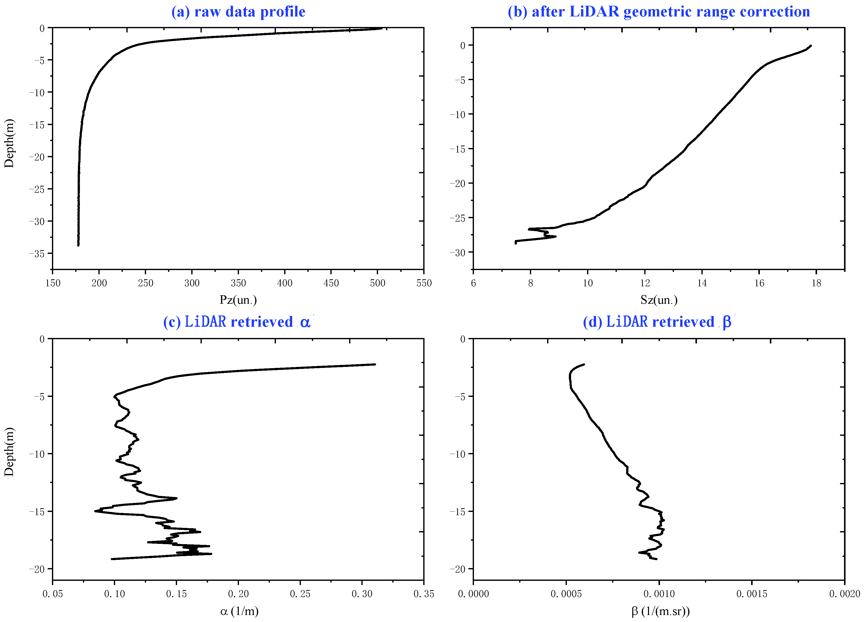
Figure 4 shows an example of the LiDAR processing results in each procedure. The LiDAR data acquired at (109°48.158′E, 18°18.309′N) on 30 September, 2017 were used to demonstrate the performance of the LiDAR processing procedure. A raw LiDAR signal profile as a function of depth is shown in Figure 4a. It seems that the LiDAR signal amplitude decreased sharply when the LiDAR pulses just entered the sea water (within 3 m depth). That was due to the water surface reflection and PMT transient response effect, and little water backscatter could be detected by the receiver. When the LiDAR pulses travelled deeper in the water column, the backscatter increased due to multiple scatterings, and the signal amplitude decreased slowly by 1% of the LiDAR amplitude as the depth increased by one meter, as illustrated in Figure 4a. Figure 4b shows the geometric range corrected LiDAR return in logarithmical form after background-noise subtraction. Figure 4c represents the retrieved α by the Klett method. The sharp decrease of α (<3 m) was eliminated to reduce the effects of the water surface reflection. Figure 4d demonstrates the retrieved β by the PR method. The attenuation coefficient of the water at this station is within 0.2 m−1. The values of LiDAR-retrieved α and β show similar levels of variability, and both increased slowly overall along the depth (>5 m).
3.2. Validation of the LiDAR Inversion Method
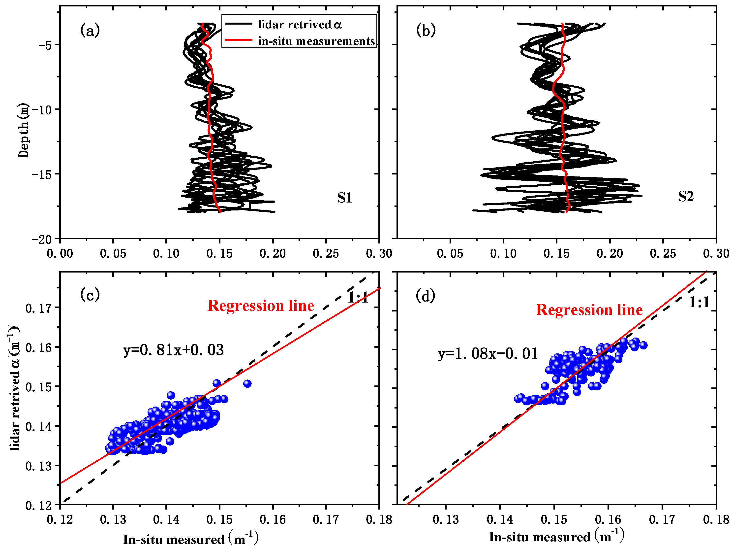
Figure 5 compares LiDAR-retrieved α by using the hybrid method with in-situ measurements at Station S1 (Figure 5a,c) and Station S2 (Figure 5b,d) in the SCS. Each in-situ measurement (red line) matches up to a total of 10 inversion profiles (black curves). We can see that the profiles of LiDAR-retrieved α and shipborne-measured water attenuation coefficients have similar levels of variability over much of the depth range (Figure 5a,b). The Pearson correlation coefficients between LiDAR-derived results and traditional measurements at S1 and S2 are 0.67 and 0.70, respectively (Figure 5c,d). The MREs at S1 and S2 are both are within 10%, at 7.1% and 9.7%, respectively. In addition, the NRMSD between the two kinds of data at S1 and S2 are both are within 12%, at 8.54% and 11.55%, respectively (Table 1). This provides some evidence that the hybrid inversion method is feasible and effective due to the relative accuracy as both are within 30%.
3.3. LiDAR Inversion Profile Distribution along LiDAR Flight Tracks
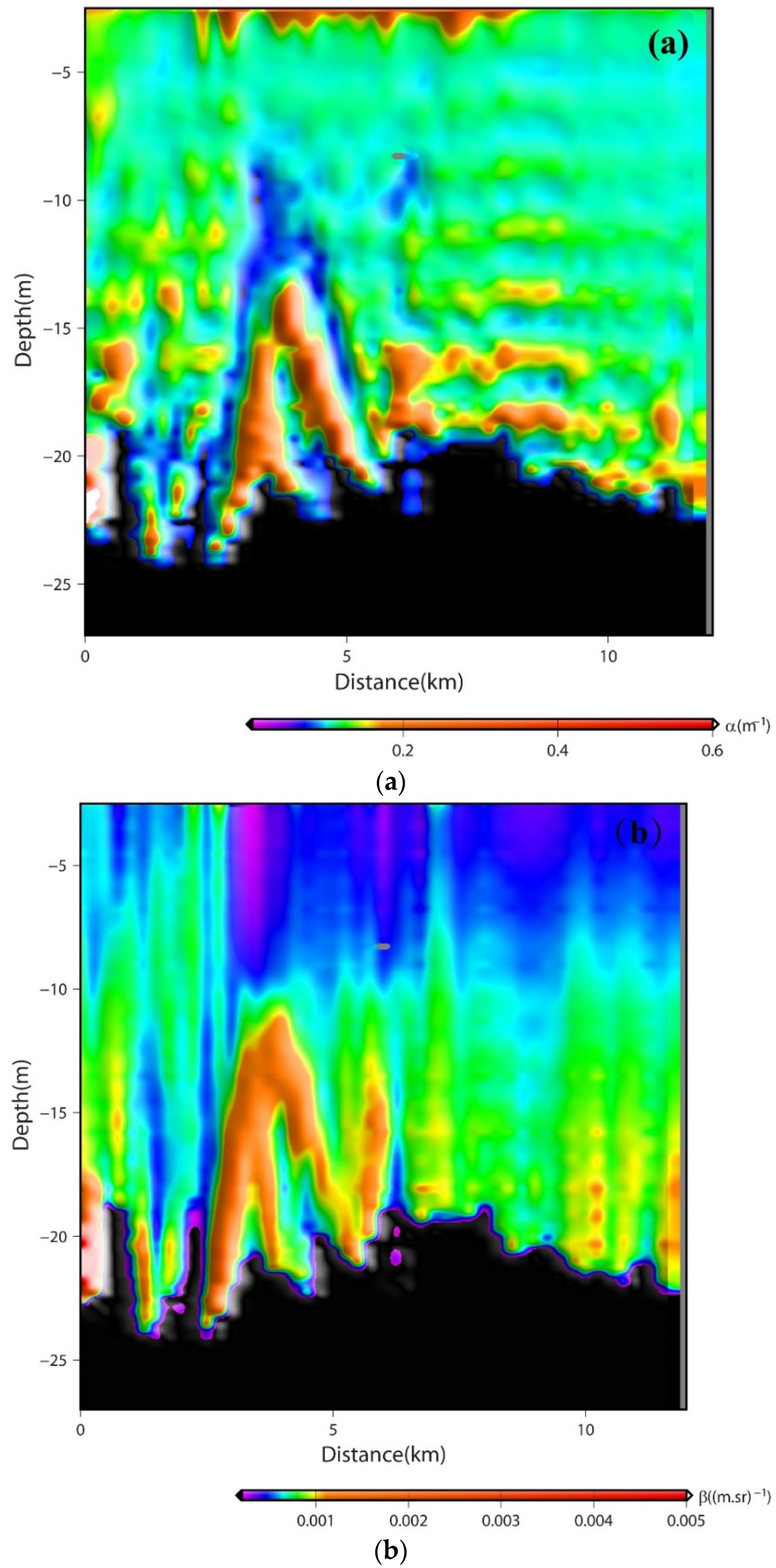
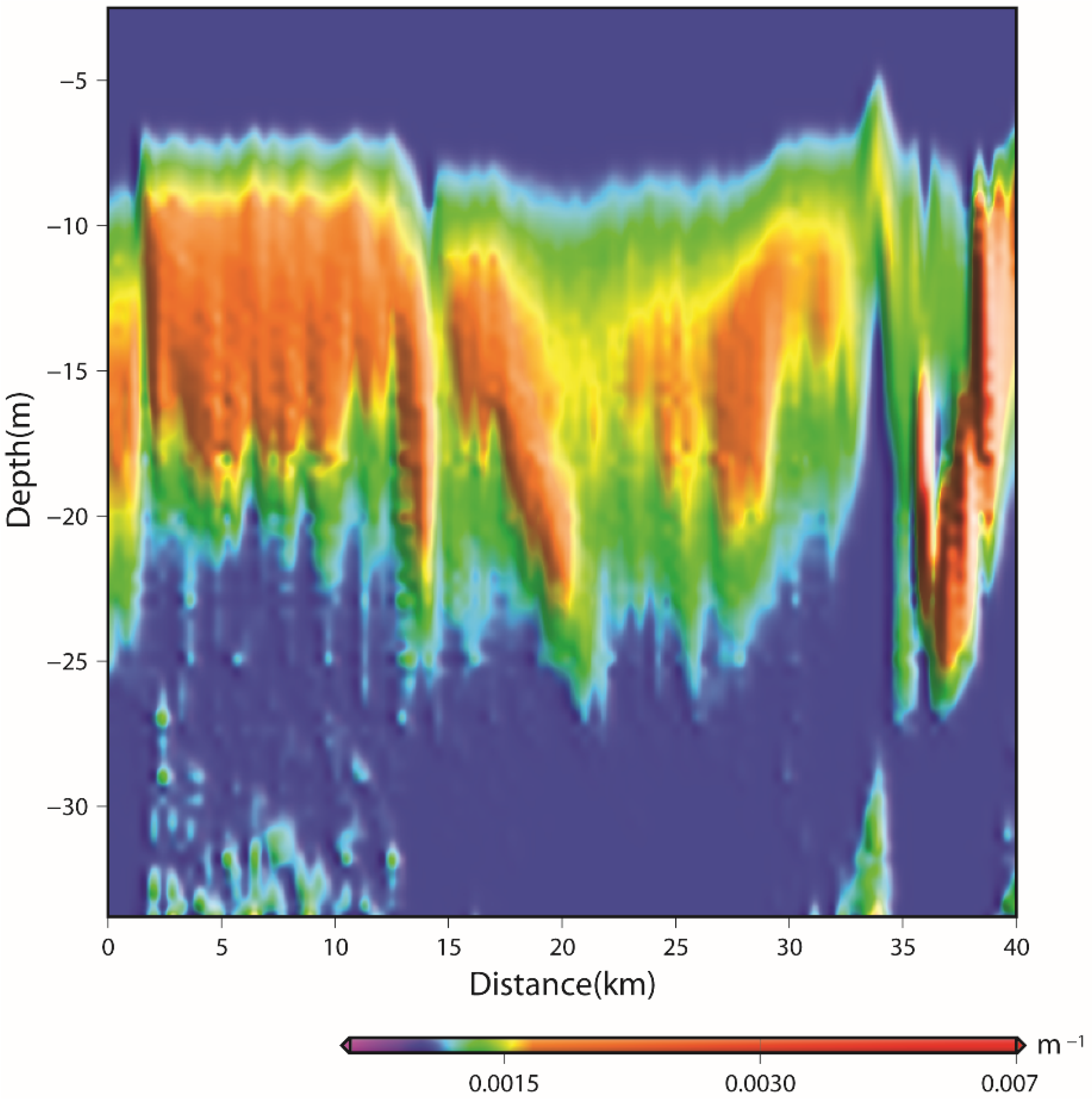
Figure 6 shows LiDAR-retrieved attenuation and backscattering profiles mapped as a function of depth and distance along the airborne LiDAR flight tracks with the color table at the bottom. Every 50 pulse amplitude were averaged, and the data were averaged to 112.5-m horizontal resolution and 0.11-m vertical resolution. Figure 6a,b show the LiDAR-retrieved α and β profiles, respectively. We can see a variety of water types and structures that were observed along the flight track. The LiDAR-derived α ranges from purple (=0.0 m−1) to red (=0.6 m−1). The LiDAR-derived β ranges from purple (=0.0001 (m.sr)−1) to red (=0.005 (m.sr)−1). The black parts are the areas when LiDAR data were not available due to the SNR being low or the LiDAR light reaching the sea floor. These data also clearly show larger values near the bottom of the depth range, which may be due to sediment movement or sea grass above the sea bottom. It indicates that we could also obtain coarse bathymetry information of shallow water along the tracks. Figure 7 shows the LiDAR-retrieved bbp in Sanya Bay water based on the bio-optical model . It shows a subsurface phytoplankton layer between 10 to 20 m depths along the flight track in Sanya Bay. Primary results demonstrated our airborne LiDAR has an ability to survey and characterize an ocean optical structure.
4. Discussion
We found that our airborne LiDAR can be successfully employed for obtaining upper water attenuation coefficients and backscattering profile information. Indeed, LiDAR has several advantages of rapid data acquisition, large area coverage over traditional shipborne observations. For instance, given the same area with 100 square kilometers, it needs more than three days for shipborne measurements (about 25 stations with 2 km between stations), while it takes less than one hour by an airborne LiDAR. Both shipborne and airborne LiDAR could provide continuous coverage survey compared with traditional discrete station observations. In addition, there is no external disturbance for phytoplankton layers when detecting them, due to the fact that the keeping thrusters on a large ship are powerful enough to disturb and mix the upper water column. Airborne LiDAR techniques can avoid the above-mentioned problem.
The LiDAR attenuation coefficient α in the LiDAR equation is an “effective” attenuation coefficient, which accounts for the effects of multiple scatterings in the water. It is not equal to the water attenuation coefficient c. Note that one needs to establish the relation between LiDAR attenuation coefficient α and water attenuation coefficient c or water diffuse attenuation coefficient Kd during different LiDAR parameters’ setup, especially for different LiDAR FOV. Previous studies showed that LiDAR-retrieved α closely approximates the c with a narrow FOV and Kd with a large FOV [23,29,30]. However, for a certain shipborne or airborne LiDAR with middle FOV, we need to build the relationship through simulation methods or comparisons between LiDAR-retrieved α and in-situ measurements of water attenuation.
The multiple scattering effect on α can also be expressed as follows, according to [31]:
where D is the spot diameter of LiDAR on the water surface, which equals the result of LiDAR altitude H multiplying FOV. It suggests that α will closely approximate Kd for cD greater than 2 or 3 and close to c for cD smaller than 0.2 [31].
In our study, because the FOV of our LiDAR system was narrow with 6 mrad, so on the water surface and c is about 0.1 m−1 in the study area; thus, . Therefore, α can be assumed as the beam attenuation coefficient c in this study. In many practical devices, it is better to choose small FOV (less than 5 mrad) to obtain c and large FOV (more than 100 mrad) to obtain Kd. Multi-FOV LiDARs are the future development trend. For a satellite LiDAR, because the spot diameter of LiDAR on the water surface is often dozens of meters [32], we can assume the LiDAR attenuation coefficient α is close to Kd. Therefore, the quasi-single scattering approximation (Equation (1)) can be an efficient method to model the performance of satellite LiDAR systems.
In this study, the LiDAR-retrieved bbp in Figure 7 is based on the bio-optical model between the bbp and volume scattering function β expressed as . The uncertainty of this bio-optical model depends on various water types. Further investigation is needed to confirm this model in various sea areas to improve and validate the model. There is a more frequently used relationship can be expressed as [33,34]:
where βp is the particulate β at 180°and χ(θ) is a conversion factor. There is also an uncertainty for this model in χ (180°). Some previous studies on LiDAR at 532 nm reports χ (180°) was about 1.43 [35], while others report χ (180°) = 0.5 [33,34,36]. A new instrument for phase scattering function measurements is required, since most of the current methods cannot be extended to 180° [37].
5. Conclusions
Our results indicated that the airborne LiDAR technique is feasible and effective for ocean optical profiling in the SCS. Primary results demonstrated that the AOL-SIOMairborne LiDAR has an independent ability to survey and characterize ocean optical structure. The maximum penetrated depth can reach 30 m by the AOL-SIOM, and subsurface phytoplankton layer could be detected, both shipborne and airborne LiDAR could provide a continuous coverage survey compared with traditional discrete station observations, which will help us to understand the upper ocean better. There are a few issues to be aware of, such as an accurate estimation of water column optical properties. The limitation of the PR technique in our hybrid method assumed that α slowly varyied with depth. One useful solution is to employ the HSRL technique which measures attenuation and scattering coefficient independently. A multi-polarization technique is also a future growth priority. Another issue is the uncertainty in LiDAR-system calibration. Our current method employed in-situ measurements into the LiDAR equation, to obtain LiDAR system constant. Improving the calibration is an ongoing effort. Further investigation is needed to confirm airborne LiDAR experiments in various water types to enhance and validate our method.
Author Contributions
Funding acquisition, Methodology, P.C.; Supervision, D.P.
Funding
This research was funded by the National Key Research and Development Program of China grant number 2016YFC1400901; the Scientific Research Fund of the Second Institute of Oceanography, State Oceanic Administration grant number QNYC1803; and the Zhejiang Natural Science Foundation grant number LQ19D060003. And the APC was funded by the National Key Research and Development Program of China grant number 2016YFC1400901.
Acknowledgments
We would like to thank the organizations that provided in-situ measurements and air-borne LiDAR data. Three anonymous reviewers provided useful comments and criticisms, which helped to improve the presentation significantly.
Conflicts of Interest
The authors declare no conflicts of interest.
References
- Hostetler, C.A.; Behrenfeld, M.J.; Hu, Y.; Hair, J.W.; Schulien, J.A. Spaceborne Lidar in the Study of Marine Systems. Annu. Rev. Mar. Sci. 2018, 10, 121–147. [Google Scholar] [CrossRef] [PubMed]
- Behrenfeld, M.J.; Hu, Y.; O’Malley, R.T.; Boss, E.S.; Hostetler, C.A.; Siegel, D.A.; Sarmiento, J.L.; Schulien, J.; Hair, J.W.; Lu, X. Annual boom–bust cycles of polar phytoplankton biomass revealed by space-based lidar. Nat. Geosci. 2016, 10, 18. [Google Scholar] [CrossRef]
- Richter, K.; Maas, H.-G. An Approach to Determining Turbidity and Correcting for Signal Attenuation in Airborne Lidar Bathymetry. J. Photogramm. Remote Sens. Geoinf. Sci. 2017, 85, 31–40. [Google Scholar] [CrossRef]
- Saylam, K.; Brown, R.A.; Hupp, J.R. Assessment of depth and turbidity with airborne Lidar bathymetry and multiband satellite imagery in shallow water bodies of the Alaskan North Slope. Int. J. Appl. Earth Obs. Geoinf. 2017, 58, 191–200. [Google Scholar] [CrossRef]
- Lee, J.H.; Churnside, J.H.; Marchbanks, R.D.; Donaghay, P.L.; Sullivan, J.M. Oceanographic lidar profiles compared with estimates from in situ optical measurements. Appl. Opt. 2013, 52, 786–794. [Google Scholar] [CrossRef]
- Kokhanenko, G.P.; Balin, Y.S.; Penner, I.E.; Shamanaev, V.S. Lidar and in situ measurements of the optical parameters of water surface layers in Lake Baikal. Atmos. Ocean. Opt. 2011, 24, 478–486. [Google Scholar] [CrossRef]
- Churnside, J.; Hair, J.; Hostetler, C.; Scarino, A. Ocean Backscatter Profiling Using High-Spectral-Resolution Lidar and a Perturbation Retrieval. Remote Sens. 2018, 10, 2003. [Google Scholar] [CrossRef]
- Concannon, B.M.; Prentice, J.E. LOCO with a Shipboard Lidar. 2008. [Google Scholar]
- Churnside, J.H.; Marchbanks, R.D. Subsurface plankton layers in the Arctic Ocean. Geophys. Res. Lett. 2015, 42, 4896–4902. [Google Scholar] [CrossRef]
- Liu, H.; Chen, P.; Mao, Z.; Pan, D.; He, Y. Subsurface plankton layers observed from airborne lidar in Sanya Bay, South China Sea. Opt. Express 2018, 26, 29134–29147. [Google Scholar] [CrossRef]
- Arnone, R.; Derada, S.; Ladner, S.; Trees, C. Probing the subsurface ocean processes using ocean LIDARS. In Proceedings of the SPIE—The International Society for Optical Engineering, Baltimore, MD, USA, 12 June 2012; Volume 8372, p. 21. [Google Scholar] [CrossRef]
- Churnside, J. Lidar signature from bubbles in the sea. Opt. Express 2010, 18, 8294–8299. [Google Scholar] [CrossRef]
- Churnside, J.D.; Marchbanks, R.H.; Lee, J.; Shaw, J.; Weidemann, A.L.; Donaghay, P. Airborne lidar detection and characterization of internal waves in a shallow Fjord. J. Appl. Remote Sens. 2012, 6, 3611. [Google Scholar] [CrossRef]
- Roddewig, M.R.; Pust, N.J.; Churnside, J.H.; Shaw, J.A. Dual-polarization airborne lidar for freshwater fisheries management and research. Opt. Eng. 2017, 56, 031221. [Google Scholar] [CrossRef] [Green Version]
- Roddewig, M.R.; Churnside, J.; Hauer, F.R.; Williams, J.; Bigelow, P.; Koel, T.; Shaw, J. Airborne lidar detection and mapping of invasive lake trout in Yellowstone Lake. Appl. Opt. 2018, 57, 4111–4116. [Google Scholar] [CrossRef] [PubMed]
- Churnside, J.H.; Marchbanks, R.D. Inversion of oceanographic profiling lidars by a perturbation to a linear regression. Appl. Opt. 2017, 56, 5228–5233. [Google Scholar] [CrossRef] [PubMed]
- Hair, J.W.; Hostetler, C.A.; Cook, A.L.; Harper, D.B.; Ferrare, R.A.; Mack, T.L.; Welch, W.; Izquierdo, L.R.; Hovis, F.E. Airborne High Spectral Resolution Lidar for profiling aerosol optical properties. Appl. Opt. 2008, 47, 6734–6752. [Google Scholar] [CrossRef] [PubMed]
- Dawson, K.W.; Meskhidze, N.; Josset, D.; Gassó, S. Spaceborne observations of the lidar ratio of marine aerosols. Atmos. Chem. Phys. 2015, 15, 3241–3255. [Google Scholar] [CrossRef] [Green Version]
- Kunz, G.J.; de Leeuw, G. Inversion of lidar signals with the slope method. Appl. Opt. 1993, 32, 3249–3256. [Google Scholar] [CrossRef] [PubMed]
- Fernald, F.G. Analysis of atmospheric lidar observations: Some comments. Appl. Opt. 1984, 23, 652–653. [Google Scholar] [CrossRef]
- Klett, J.D. Stable analytical inversion solution for processing lidar returns. Appl. Opt. 1981, 20, 211–220. [Google Scholar] [CrossRef] [Green Version]
- Churnside, J.H.; Sullivan, J.M.; Twardowski, M.S. Lidar extinction-to-backscatter ratio of the ocean. Opt. Express 2014, 22, 18698–18706. [Google Scholar] [CrossRef]
- Chen, P.; Pan, D.; Mao, Z.; Liu, H. Semi-analytic Monte Carlo radiative transfer model of laser propagation in inhomogeneous sea water within subsurface plankton layer. Opt. Laser Technol. 2019, 111, 1–5. [Google Scholar] [CrossRef]
- Mitchell, B.G.; Kahru, M.; Wieland, J.; Stramska, M. Determination of spectral absorption coefficients of particles, dissolved material and phytoplankton for discrete water samples. Nasa Tech. Memo. 2002, 125–153. [Google Scholar]
- Kopilevich, Y.I.; Surkov, A.G. Mathematical modeling of the input signals of oceanological lidars. J. Opt. Technol. 2008, 75, 321–326. [Google Scholar] [CrossRef]
- Chen, P.; Pan, D.; Mao, Z.; Liu, H. A Feasible Calibration Method for Type 1 Open Ocean Water LiDAR Data Based on Bio-Optical Models. Remote Sens. 2019, 11, 172. [Google Scholar] [CrossRef]
- Sullivan, J.M.; Twardowski, M.S. Angular shape of the oceanic particulate volume scattering function in the backward direction. Appl. Opt. 2009, 48, 6811–6819. [Google Scholar] [CrossRef] [PubMed]
- PinEiro, G.; Perelman, S.; Guerschman, J.P.; Paruelo, J.M. How to evaluate models: Observed vs. predicted or predicted vs. observed? J. Ecol. Model. 2008, 216, 316–322. [Google Scholar] [CrossRef]
- Gordon, H.R. Interpretation of airborne oceanic lidar: Effects of multiple scattering. Appl. Opt. 1982, 21, 2996–3001. [Google Scholar] [CrossRef] [PubMed]
- Walker, R.E.; McLean, J.W. Lidar equations for turbid media with pulse stretching. Appl. Opt. 1999, 38, 2384–2397. [Google Scholar] [CrossRef]
- Churnside, J.H. Review of profiling oceanographic lidar. Opt. Eng. 2014, 53, 051405. [Google Scholar] [CrossRef]
- Winker, D.; Pelon, J.; Coakley, J., Jr.; Ackerman, S.; Charlson, R.; Colarco, P.; Flamant, P.; Fu, Q.; Hoff, R.; Kittaka, C. The CALIPSO mission: A global 3D view of aerosols and clouds. Bull. Am. Meteorol. Soc. 2010, 91, 1211–1230. [Google Scholar] [CrossRef]
- Boss, E.; Pegau, W.S. Relationship of light scattering at an angle in the backward direction to the backscattering coefficient. Appl. Opt. 2001, 40, 5503–5507. [Google Scholar] [CrossRef] [PubMed]
- Chami, M.; Marken, E.; Stamnes, J.; Khomenko, G.; Korotaev, G. Variability of the relationship between the particulate backscattering coefficient and the volume scattering function measured at fixed angles. J. Geophys. Res. Ocean 2006, 111. [Google Scholar] [CrossRef]
- Zhang, X.; Boss, E.; Gray, D.J. Significance of scattering by oceanic particles at angles around 120 degree. Opt. Express 2014, 22, 31329–31336. [Google Scholar] [CrossRef] [PubMed]
- Whitmire, A.L.; Pegau, W.S.; Karp-Boss, L.; Boss, E.; Cowles, T.J. Spectral backscattering properties of marine phytoplankton cultures. Opt. Express 2010, 18, 15073–15093. [Google Scholar] [CrossRef] [PubMed] [Green Version]
- Churnside, J.H.; Marchbanks, R.D.; Lembke, C.; Beckler, J. Optical backscattering measured by airborne lidar and underwater glider. Remote Sens. 2017, 9, 379. [Google Scholar] [CrossRef]
Figure 1.
Diagram of the major optoelectronic components (a), and a picture of the LiDAR (b).

Figure 2.
LiDAR flight experiments in the SCS. The color lines are flight tracks of airborne LiDAR taken on 23 September (black) and 30 September (blue), 2017, and on 11 March (red) and 12 March (green), 2018.
Figure 2.
LiDAR flight experiments in the SCS. The color lines are flight tracks of airborne LiDAR taken on 23 September (black) and 30 September (blue), 2017, and on 11 March (red) and 12 March (green), 2018.

Figure 3.
Flow chart showing the inversion process.

Figure 4.
An example of processing the LiDAR data acquired on 30 September, 2017. (a) The profile from the raw LiDAR data, (b) the geometric range corrected LiDAR return in logarithmical form after background-noise subtraction, (c) the profile from the retrieved α, and (d) the profile from the retrieved β.

Figure 5.
Comparison of airborne LiDAR-derived results with traditional measurements. (a,c) are the comparison results for S1; (b,d) are the comparison results for S2.
Figure 5.
Comparison of airborne LiDAR-derived results with traditional measurements. (a,c) are the comparison results for S1; (b,d) are the comparison results for S2.

Figure 6.
LiDAR-retrieved attenuation and backscattering vertical structure distribution. α ranges from purple (=0.0 m−1) to red (=0.6 m−1). β ranges from purple (=0.0001 (m.sr)−1) to red (=0.005 (m.sr)−1).
Figure 6.
LiDAR-retrieved attenuation and backscattering vertical structure distribution. α ranges from purple (=0.0 m−1) to red (=0.6 m−1). β ranges from purple (=0.0001 (m.sr)−1) to red (=0.005 (m.sr)−1).

Figure 7.
LiDAR-retrieved bbp vertical structure distribution in Sanya Bay water, ranges from purple (=0.0 m−1) to red (=0.007 m−1).
Figure 7.
LiDAR-retrieved bbp vertical structure distribution in Sanya Bay water, ranges from purple (=0.0 m−1) to red (=0.007 m−1).


Table 1.
The curve-fitting statistics between LiDAR inversion and in-situ measurements.
| Station | Number | Min | Max | R | MAE | RMSE | NRMSD |
|---|---|---|---|---|---|---|---|
| 1 | 260 | 0.128 | 0.143 | 0.67 | 7.1% | 0.012 | 8.54% |
| 2 | 130 | 0.156 | 0.166 | 0.70 | 9.7% | 0.018 | 11.55% |
© 2019 by the authors. Licensee MDPI, Basel, Switzerland. This article is an open access article distributed under the terms and conditions of the Creative Commons Attribution (CC BY) license (http://creativecommons.org/licenses/by/4.0/).
Share and Cite
MDPI and ACS Style
Chen, P.; Pan, D. Ocean Optical Profiling in South China Sea Using Airborne LiDAR. Remote Sens. 2019, 11, 1826. https://0-doi-org.brum.beds.ac.uk/10.3390/rs11151826
AMA Style
Chen P, Pan D. Ocean Optical Profiling in South China Sea Using Airborne LiDAR. Remote Sensing. 2019; 11(15):1826. https://0-doi-org.brum.beds.ac.uk/10.3390/rs11151826
Chicago/Turabian StyleChen, Peng, and Delu Pan. 2019. "Ocean Optical Profiling in South China Sea Using Airborne LiDAR" Remote Sensing 11, no. 15: 1826. https://0-doi-org.brum.beds.ac.uk/10.3390/rs11151826
Note that from the first issue of 2016, this journal uses article numbers instead of page numbers. See further details here.