Evaluation of Grass Quality under Different Soil Management Scenarios Using Remote Sensing Techniques

1
Department of Soil Science, Faculty of Agriculture, University of Zanjan, 45371-38791 Zanjan, Iran
2
National Centre for Geocomputation, Maynooth University, Maynooth, Co. Kildare W23 F2K8, Ireland
3
Teagasc, Animal & Grassland Research and Innovation Centre, Moorepark, Co. Cork P61 C996, Ireland
4
Department of Process, Energy and Transport Engineering, Cork Institute of Technology, Cork T12 P928, Ireland
*
Author to whom correspondence should be addressed.
Remote Sens. 2019, 11(15), 1835; https://0-doi-org.brum.beds.ac.uk/10.3390/rs11151835
Submission received: 18 July 2019
/
Revised: 2 August 2019
/
Accepted: 3 August 2019
/
Published: 6 August 2019
(This article belongs to the Section Remote Sensing in Agriculture and Vegetation)
Abstract
:Hyperspectral and multispectral imagery have been demonstrated to have a considerable potential for near real-time monitoring and mapping of grass quality indicators. The objective of this study was to evaluate the efficiency of remote sensing techniques for quantification of aboveground grass biomass (BM) and crude protein (CP) in a temperate European climate such as Ireland. The experiment was conducted on 64 plots and 53 paddocks with varying quantities of nitrogen applied. Hyperspectral imagery (HSI) and multispectral imagery (MSI) were analyzed to develop the prediction models. The MSI data used in this study were captured using an unmanned aircraft vehicle (UAV) and the satellite Sentinel-2, while the HSI data were obtained using a handheld hyperspectral camera. The prediction models were developed using partial least squares regression (PLSR) and stepwise multi-linear regression (MLR). Eventually, the spatial distribution of grass biomass over plots and paddocks was mapped to assess the within-field variability of grass quality metrics. An excellent accuracy was achieved for the prediction of BM and CP using HSI (RPD > 2.5 and R2 > 0.8), and a good accuracy was obtained via MSI-UAV (2 < RPD < 2.5 and R2 > 0.7) for the grass quality indicators. The accuracy of the models calculated using MSI-Sentinel-2 was reasonable for BM prediction and insufficient for CP estimation. The red-edge range of the wavelengths showed the maximum impact on the predictability of grass BM, and the NIR range had the greatest influence on the estimation of grass CP. Both the PLSR and MLR techniques were found to be sufficiently robust for spectral modelling of aboveground BM and CP. The PLSR yielded a slightly better model than MLR. This study suggested that remote sensing techniques can be used as a rapid and reliable approach for near real-time quantitative assessment of fresh grass quality under a temperate European climate.
1. Introduction
Grasslands are the dominant land-cover type in Ireland and are the most productive agricultural lands in the world [1,2,3]. Grassland management operations play an important role in the sustainability of forage productivity [4,5]. The quality of grass consumed by livestock is an important parameter for beef and dairy productivity. Grass quality can usually be measured and assessed by indicators such as grass biomass [6], height [7], density, and crude protein [8]. Aboveground grass biomass, which is usually measured as kilograms grass dry matter (DM) produced per hectare (kg DM ha−1) and crude protein (g kg−1 DM), are considered important indicators for assessing fresh grass quality (GQ) and the efficiency of fertilization management systems during the growing season [9].
High spatiotemporal variability is an important issue in monitoring and managing GQ [10]. The differences in soil, topography, weather conditions, species composition, and management practices are the main reasons for GQ variation during the growing season [11,12]. To account for these variations, a large quantity of seasonal data is usually required for evaluating and mapping GQ indicators. Well-established methodologies for assessing GQ indicators include wet chemistry and laboratory-based methods, which are laborious, time-consuming, and expensive [13]. On the other hand, point spectroscopic techniques have been reported in the literature as rapid tools for monitoring GQ (e.g., [11,13,14]), but these techniques remain relatively expensive and require considerable expertise [15]. Accordingly, developing a non-destructive, rapid, and reliable approach for spatiotemporal modelling of fresh grass quantity and quality would make a substantial contribution to sustainable grassland management practices.
Over the past three decades, imagery and remote sensing techniques have been reported to be an effective alternative to the conventional field and laboratory analyses [16,17]. The assessment of GQ can be carried out at different scales from global and regional to farm and individual paddocks [1]. Depending on the selected spatial scales, airborne optical sensors with specific spectral characteristics can be used for reliable prediction of grass growth parameters. Although higher-level satellite images are useful for evaluating large areas, their spatial resolution is often too coarse for more precise estimation of GQ attributes owing to the smaller spatial size of grassland paddocks [18]. For a farm scale assessment of GQ during a typical growing season, high spatiotemporal resolution is essential to detect within-field variations [19]. Cloud cover and atmospheric noise can hamper and significantly impact the wider usefulness of satellite imagery, particularly in a temperate maritime climate such as Ireland. Atmospheric corrections and the use of unmanned aircraft vehicle (UAV) imagery have been suggested as routine approaches to cope with these issues [20]. Visible (VIS) and near infrared (NIR) spectra have been demonstrated to have a significant correlation with certain plant growth attributes [21]. The vegetation spectral signatures of photosynthetic pigments in the VIS range and the absorbance spectra of water, nitrogen concentration, and protein in the NIR range can be associated with the spectral predictability of plant vitality indicators [22]. In addition to the specific spectral bands, several spectral indices have been suggested as practical indices for quantification of plant biophysical attributes such as the normalized difference vegetation index (NDVI), normalized difference red-edge (NDRE), and chlorophyll index (CI) [2,23]. Spectral indices can reduce the background noise and enhance the accuracy of prediction models [23,24]. A broad range of spectral bands acquired using different remote sensing systems, particularly hyperspectral images, can help to identify the useful wavelength ranges for predicting GQ indicators and to improve the accuracy of spectral models substantially.
The combination of multispectral and hyperspectral remote sensing imagery with in situ analysis and local knowledge provides a valuable framework for evaluating the impact of management operations on grass characteristics and to monitor the variation of biomass (BM) and crude protein (CP) over a period of time [25,26]. The application of hyperspectral data can significantly improve the accuracy of prediction models related to plant studies [27]. A larger number of narrow wavelength bandwidths, covering a wider spectral range, recorded by hyperspectral sensors provide a better opportunity for estimating grass parameters [28]. Recent developments in airborne and space-borne remote sensing along with improvements in the image quality in terms of spatial, spectral, temporal, and radiometric resolution have enabled more accurate prediction of plant attributes associated with forage quality [26,29]. Despite the improved potential of remote sensing imagery for evaluating GQ, the efficiency of these techniques for an accurate prediction of aboveground grass BM and CP as important indicators of GQ remains unclear, and few studies have been reported on “grass-based food security” [26]. A comprehensive study on the efficiency of multispectral and hyperspectral data captured using different remote sensing techniques (satellite, UAV, and fixed ground-based platform imagery) is of particular interest in helping identify optimal wavelengths, robust modelling approaches, and significant spectral indices for predicting and mapping fresh GQ indicators.
Multivariate analyses have been reported as practical statistical approaches for spectral modelling of plant biomass [30,31]. The partial least squares regression (PLSR) and stepwise multiple linear regression (MLR) models are the most common regression techniques which have been reported as practical approaches for spectral analyses [32,33]. The capability of these two techniques for predicting fresh GQ indicators in the temperate maritime climate in Ireland was assessed in this study. The main aim was to evaluate the efficiency of hyperspectral and multispectral (UAV and satellite) remote sensing techniques for predicting and mapping grass BM and CP under conventional grassland management in a temperate maritime climate. This aim was supported by two objectives: (a) to identify optimal wavelengths and spectral indices for estimating grass BM and CP and (b) to determine the most appropriate regression approach (stepwise MLR or PLSR) for developing prediction models. To the best of our knowledge, the ability of different imaging sensor system configuration (UAV-based MSI, satellite-based MSI, and fixed ground-based HSI) for capturing and mapping GQ in a temperate maritime grassland environment, such as Ireland, has not been adequately researched.
2. Materials and Methods
2.1. Experimental Design
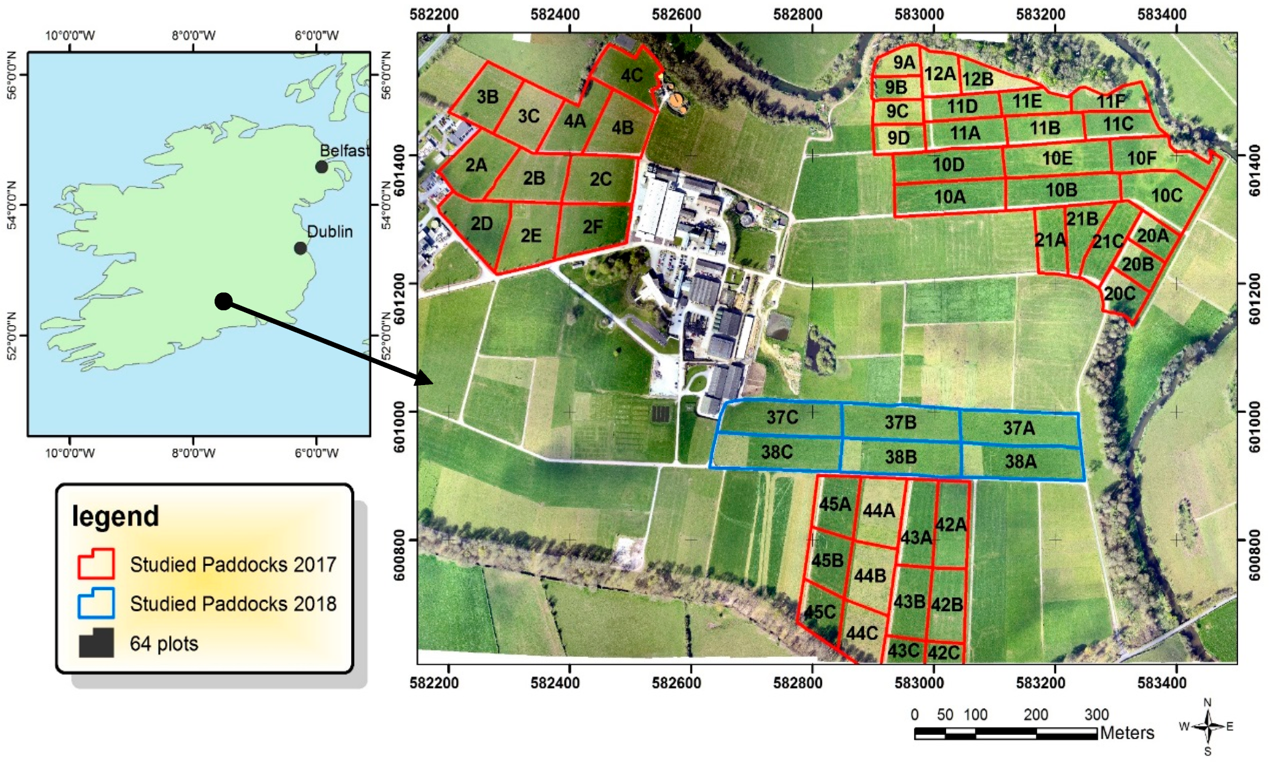
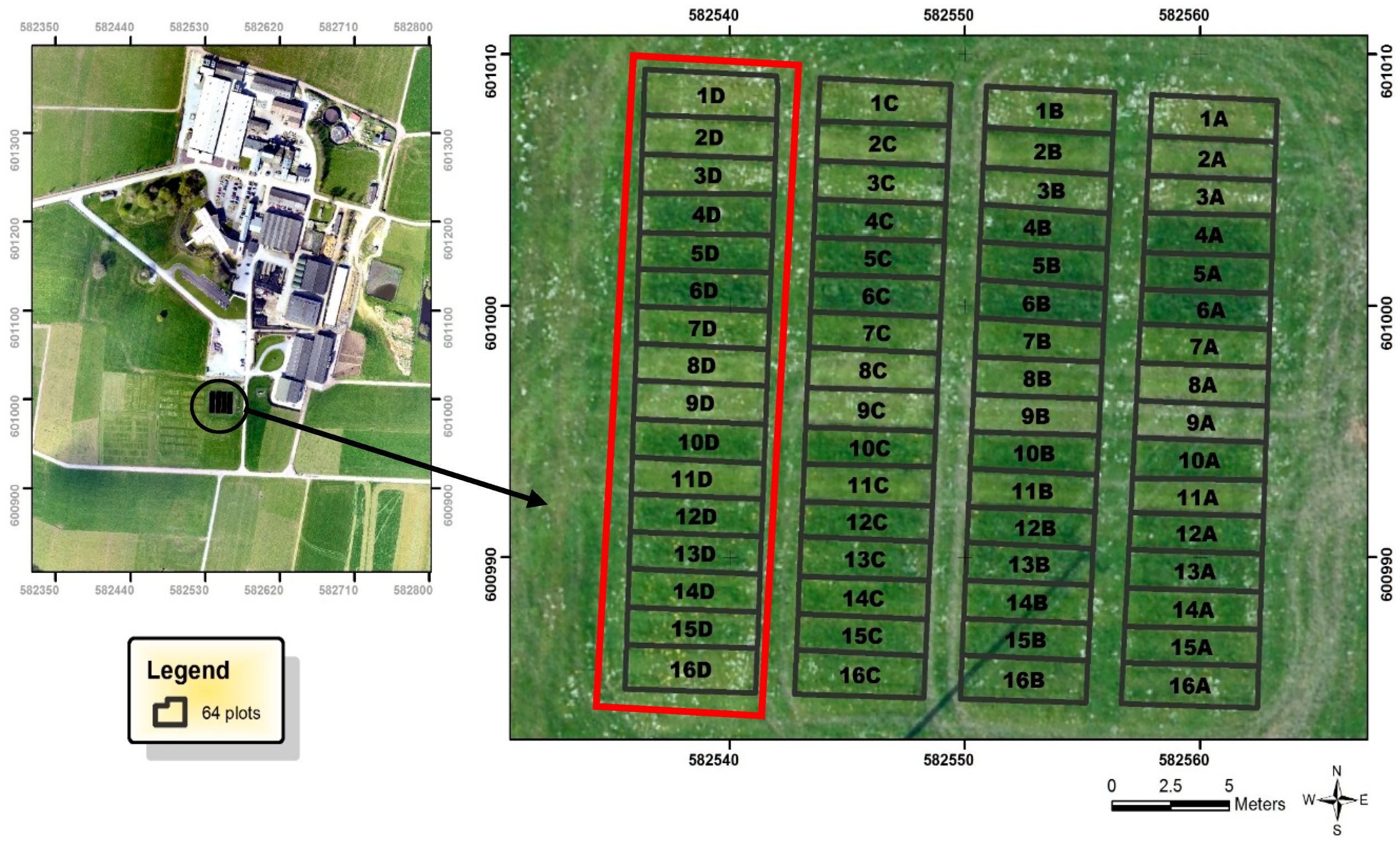
The study was conducted in Ireland during 2017 and 2018 (Figure 1, Moorepark TEAGASC research center in Fermoy, Cork) where grassland plots and paddocks were chosen as a representative sample of a typical Irish grassland management system. The soil in the study area is typically classified as Grey–Brown Podzolic with a sandy loam texture. This region has an average precipitation of 1016.5 mm and mean monthly temperature values ranging from 5 °C to 20 °C. Field trials commenced in early 2017 when 64 controlled plots (5 m × 1.25 m; Figure 2) along with 53 paddocks were selected to measure grass BM and CP (Figure 1). The plots and paddocks were managed using different levels of nitrogen applied resulting in variable grass growth and quality (Table 1). A mixture of clover (Trifolium repens L.) and perennial ryegrass (Lolium perenne) (typically with a rate of 30% clover) was identified as the dominant vegetation cover in the studied sites. Three imagery systems were employed to assess the efficiency of remote sensing techniques for monitoring and mapping GQ indicators. These imaging systems included a multi-spectral Sequoia sensor, a Bay Spec hyperspectral camera, and Sentinel-2 images, where these systems produced three spectral datasets (presented in Table 2). These spectral datasets consisted of multispectral imagery (MSI) captured using a UAV, hyperspectral imagery (HSI), and Sentinel-2 multispectral imagery (MSI-Sentinel-2).
2.2. Spectral Datasets
2.2.1. MSI-UAV Dataset
The UAV study was carried out on plots in 2017 (Figure 2) and data acquisition continued for the growing season in 2018 on large-scale grazed paddocks (Figure 1, blue boundaries). The Sequoia sensor, which has four multispectral bands (Table 2), was deployed on a rotary UAV to acquire multispectral images on six dates; in 2017 (15 May, 12 June, 26 June, 24 July, 21 August, and 18 September) over 64 plots (1(A) to 16(D); Figure 2); and two dates in 2018 (20 April and 11 July) from six paddocks (37(A) to 38(C); Figure 1). The UAV was operated manually due to the presence of nearby obstructions and four flight lines were flown at a typical ground speed of 2 m/s over plots, resulting in 75% overlap and imagery captured every 2 s. The UAV images over 64 studied plots (1(A) to 16(D), Figure 2) were captured from 30 m above ground level and 120 m above ground level over the paddocks (37(A) to 38(C); Figure 1, blue boundary).
2.2.2. HSI Dataset
This dataset was captured on six dates in 2017 (15 May, 12 June, 26 June, 24 July, 21 August, and 18 September) using a hyperspectral sensor (OCI-F-Imager), produced by BaySpec Inc., USA, with 124 bands. The OCI imager is a “push-broom” sensor which records the images with a spectral resolution of 4.03 nm between 450 to 950 nm wavelength range (Table 2). The hyperspectral camera was attached to a hand-held mount, and the images were acquired one meter above the ground with forty-five frames per second by an operator at walking pace. BaySpec’s SpecGrabber software (BaySpec, Inc., USA) was used to control hyperspectral imager and to acquire HSI data. A white surface of Teflon with 8 cm diameter was utilized to acquire the white reference image, and the dark reference image was captured by covering the camera lens. These images were used to calibrate the intensity of the raw image. Due to the 0.3 meter swath width (18° FOV) and the difficulty of image alignment for the BaySpec imager, data were recorded over 16 plots (1(D) to 16(D), Figure 2, red boundary).
2.2.3. MSI-Sentinel-2 Dataset
The Sentinel-2 imagery (Level 2A products), which was either cloud-free or containing less than 30 percent cloud cover, were retrieved and downloaded in 2017 and 2018. Suitable Sentinel-2 data, that had zero cloud cover, over the Moorepark test site, was selected for spectral modelling over the following dates: 12 March 2017, 11 May 2017, 20 June 2017, 18 August 2017, and 7 November 2017, 21 April 2018, and 16 May 2018. Forty-seven paddocks in 2017 (Figure 1, red boundary) and six paddocks in 2018 (Figure 1, blue boundary) were tested and assessed in order to develop MSI-Sentinel-2 models.
2.3. Grass Sampling and Measurements
Grass sample cuttings were harvested from 64 plots (Figure 2) using an Etesia mechanical mower (Etesia UK Ltd. Warwick, UK), where 4 cm of grass was cut from each plot. The samples were weighed and analyzed for DM in Moorepark’s Grassland Laboratory, as described by McEvoy et al. [34]. One hundred grams of each grass subsample was weighed and oven dried at 60 °C for 48 h. The CP was determined by a LECO FP-528 (Leco Corporation, St. Joseph, MI, USA) according to the method 990-03 published by the Association of Analytical Chemists [35]. The grass sample cuts collected over plots were divided into two groups: one group of samples (G1, n = 84) for HSI modelling and the other group (G2, n = 109) for MSI-UAV modelling. Grass samples were collected just after capturing HSI and MSI-UAV images on each date detailed above.
Grass sampling over paddocks (Figure 1) was carried out at controlled reference points in each paddock. The paddocks were sub-divided into 22.25 m × 50 m test areas using Open Source QGIS 2.18.16 software, prior to sampling, which utilized a random point generation tool. Reference points (18/ha) were located in the field using a Trimble Catalyst GPS receiver (Trimble Inc., Sunnyvale, CA, USA) with a positional accuracy of ±30 cm. Grass cuts were taken and assessed in the laboratory for measuring BM and CP similar to the process detailed above. The samples collected over paddocks could also be categorized into three groups: (i) samples (G3, n = 17) collected from paddocks (37A, 37B, 37C and 38A, 38B, 38C) on 20 April 2018 and 11 July 2018, for MSI-UAV models over a larger scale; (ii) samples (G4, n = 61) collected in 2017 over 47 paddocks (Figure 1, red boundaries); and (iii) sampling (G5, n = 115) conducted in 2018 over 6 paddocks (Figure 1, blue boundaries). The G4 and G5 were used for MSI-Sentinel-2 modelling.
Overall, five sets of grass samples (G1, G2, G3, G4, and G5) were used to develop the prediction models of grass BM and CP using three imagery systems (HSI, MSI-UAV, and MSI-Sentinel-2).
2.4. Image Processing
Prior to spectral modelling, geomatic and radiometric corrections were performed on spectral datasets. Band 1, band 9, and band 10 of Sentinel-2 were not included in the MSI-Sentinel-2 models because of their relatively coarse spatial resolution (60 m) for this research. MSI-Sentinel-2 images are available at 10 and 20 m resolution. The 20 m dataset was resampled to 10 m using the “special resampling” procedure using the ENVI software [36,37] in order to handle the spatial resolution disparity and enable both datasets to be combined. Twenty-one spectral indices which had been reported as typical vegetation indices for assessing vegetation quality parameters in the published literature were selected for spectral prediction of measured grass BM and CP (Table 3). Calculated indices included; NDVI, NDRE, MTVI (Modified Triangular Vegetation Index), MCAR (Modified Chlorophyll Absorption Ratio Index), MNLI (Modified Non-Linear Index), GNDVI (Green Normalized Difference Vegetation Index), SAVI (Soil Adjusted Vegetation Index), LCI (Leaf Chlorophyll Index), MTCI (MERIS Terrestrial Chlorophyll Index), NRI (Nitrogen Reflectance Index), PSRI (Plant Senescence Reflectance Index), CI-Red-edge (Red-Edge Chlorophyll Index), CI-Green (Green Chlorophyll Index), NLI (Non-Linear Index), and seven ratio vegetation indices (Table 3, SR1 to SR7).
2.5. Developing Spectral Models Using HSI
Eighty-four grass samples (G1) were used to develop HSI models. The optimal wavelengths for modelling grass biomass were identified using Martens’ uncertainty test [52]. Variable selection is a conventional approach to improve the prediction accuracy of calibration models developed using spectral datasets. There are various methods that can be used for selecting the relevant spectral variables, such as Martens’ uncertainty test [52], variable importance in the projection [53], genetic algorithm [54], and backward interval PLS [55]. Each method has advantages and disadvantages. For instance, in the case of genetic algorithms, there is a high risk of overfitting and a valid initial model is required for backward interval PLS and variable importance in the projection [55]. The efficacy of variable selection methods varies with the dataset and, therefore, one specific method cannot always be considered superior to other methods [56]. Martens’ uncertainty test is a widely used technique for selecting spectral bands [56,57]. It is based on the “Jack-knife” resampling, which is usually used for significance testing of spectral models, and its result is easy to interpret graphically [52]. The dataset was partitioned into calibration and validation sets using a random sampling approach. Fifty-six spectral samples were used for calibration and twenty-eight samples for subsequent validation assessment. The MLR and PLSR were employed to develop spectral prediction models. The PLSR and MLR are popular regression techniques for developing spectral prediction in agricultural land use [29,58]. They are relatively easy to understand and implement compared to machine learning techniques and are practical chemometric analyses for spectral estimation of plant attributes [32,33]. The PLSR models were developed using a cross-validated approach, with 10 latent factors, on the calibration sets. Latent factors are linear integrations of variables calculated through the partial least squares procedure [57], which are used as independent components for estimating dependent indicators (BM and CP). The MLR modelling was carried out using a forward and backward stepwise approach, as already explained in detail by Martínez Gila et al. [59]. The models were independently validated using the validation dataset. A sequence of processing, including model fitting and statistical assessment of model accuracy, was further undertaken.
2.6. Developing Spectral Models Using MSI (UAV and Sentinel-2)
The MSI-UAV prediction models were developed using a total number of 128 samples collected during 2017 and 2018 from plots and paddocks (G2 and G3). The MSI-Sentinel-2 models were produced using 176 grass samples on selected paddocks in 2017 and 2018 (G4 and G5). An outlier detection approach was performed to enhance the accuracy of the prediction models. Accordingly, Hotelling’s T-squared distribution versus squared prediction error was employed. Hotelling’s T-squared test is a commonly used approach to detected outliers [60]. Specifically, five percent Hotelling’s T-squared statistic [61] was used to identify outlier data and, therefore, 2 samples identified as outlier samples were excluded from the MSI-UAV dataset. The remaining samples in each dataset (MSI-UAV and MSI-Sentinel-2) were partitioned into calibration (70%) and validation sets (30%) using the random sampling approach. For MSI-UAV models, 89 samples were used for calibration and 37 samples for the validation models. For the MSI-Sentinel-2 models, 123 samples were used for calibration and 53 samples for the validation models. The mean difference and homogeneity of variance between calibration and validation sets were also examined. The PLSR and MLR techniques were employed to calculate MSI models. The PLSR modelling was performed based on the cross-validation approach using the calibration sets, with 10 latent factors. Significant bands and spectral indices for PLSR models were identified using Martens’ uncertainty test [52]. The important bands and spectral indices for the MLR models were selected through stepwise and correlation analyses.
2.7. Evaluation of Spectral Models
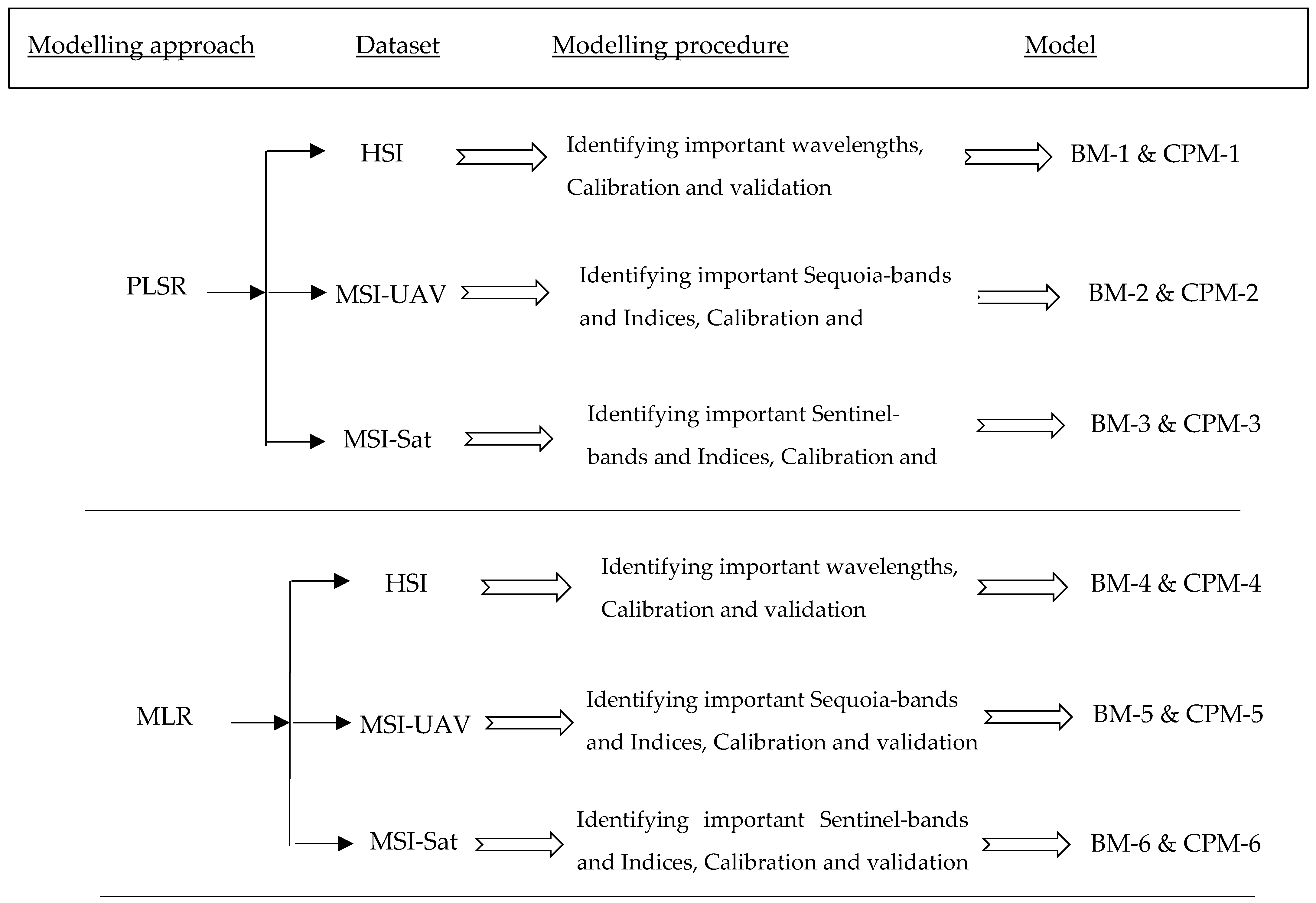
Finally, six spectral models for predicting grass biomass (BM-1 to BM-6) and six models for estimating crude protein (CPM-1 to CPM-6) were calculated using PLSR and MLR and based on HSI, MSI-UAV, and MSI-Sentinel-2 (Figure 3). Root mean square error of prediction (RMSEP), the coefficient of determination (R2), and the ratio of predicted deviation (RPD) were used to evaluate the PLSR and MLR models. The RPD was computed using Equation (1).
where Sd is the standard deviation of the reference data and SEP is the standard deviation of the prediction residuals.
RPD = Sd/SEP
In addition, the paired t-test [57] and the Pitman–Morgan test [62,63] were conducted between actual GQ indicators (measured DM and CP) and spectral predicted variables (predicted DM and CP) for validation datasets to assess the inter-variability of predicted values. These two tests were used as a complement to the more commonly used statistical tests, and to determine objectively whether the distribution variances and means of spectral predicted values were significantly different from the actual values of grass BM and CP [64].
2.8. Statistical Analysis and Mapping Indicators
The normality of measured biomass was examined using the analysis of histograms and the Kolmogorov–Smirnov test. The homogeneity of variance between calibration and validation datasets was tested using Levene’s test. All pre-processing and statistical analyses for PLSR were performed using Unscambler software (version X10.4.1; CAMO software, Woodbridge, NJ, USA). The MLR was done with SPSS v. 21 (SPSS Inc.). The paired t-test, the Pitman–Morgan test, and other analyses were carried out with R software (R x64 3.5.1) and SPSS software. Spectral prediction maps and spatial distribution of GQ indicators over the studied plots and paddocks were calculated using GIS software (QGIS 2.18.10 and ArcGIS 10.5.1).
3. Results
The characteristics of the three spectral datasets (i.e., HSI, MSI-UAV, and MSI-Sentinel 2) are summarized in Table 2, and the statistical parameters of BM and CP measured using grass samples are presented in Table 4. The HSI dataset had the maximum spectral (124 bands, 450 to 950 nm) and spatial resolution (5 mm). Four spectral bands were captured for the MSI-UAV dataset with a spatial resolution of 2.9 cm on trial plots and 11.3 cm on paddocks, with the specific wavelength ranges of green, red, red-edge, and NIR (Table 2). The MSI-Sentinel-2 had a lower spatial resolution (10 or 20 m) and a higher spectral resolution (10 bands used in this study) than MSI-UAV. Five groups of grass samples (Table 4, G1 to G5) were taken from plots and paddocks on different dates during 2017 and 2018 to obtain various ranges of CP and BM. The HSI models were calculated using G1; MSI-UAV models were developed using G2 and G3; and MSI-Sentinel-2 models were calculated employing G4 and G5 (Table 4). Overall, the ranges of measured GQ indicators for all five groups of samples were as follows: grass BM of 304–8338 kg DM ha−1 and grass CP of 126–209 g kg−1 DM. Due to the wet and cloudy conditions and absence of enough light, UAV images captured on 15 May 2017 and 26 June 2017 were excluded from MSI-UAV modelling to maintain the homogeneity of radiation. The weather condition information for Moorepark Research Centre indicated a very low global radiation (approximately 650 J/cm sq) for these two dates compared to other dates (approximately 2000 J/cm sq). Prior to the development of spectral models, datasets were separated into calibration and validation sets for independent validation of spectral models. According to the Levene’s test results, there was no significant difference between variance values of BM and CP between calibration and validation sets. The mean comparison result was also confirmed by the similarity of DM and CP mean values between validation and calibration. Accordingly, the sample distribution was appropriately represented by the validation set for all datasets. Formulas of 20 spectral indices used for developing prediction models are presented in Table 3. These spectral indices are commonly reported indices for assessing herbage quality in published literature. According to studies published by Askari et al. [5] and Viscarra-Rossel [65], spectral prediction models can be classified into excellent (RPD ≥ 2.5 and R2 ≥ 0.8), good (2 ≤ RPD < 2.5 and R2 ≥ 0.7), moderate (1.5 ≤ RPD < 2 and R2 ≥ 0.6) and poor accuracy (RPD < 1.5 and R2 < 0.6).
3.1. Predicting GQ Indicators Using PLSR
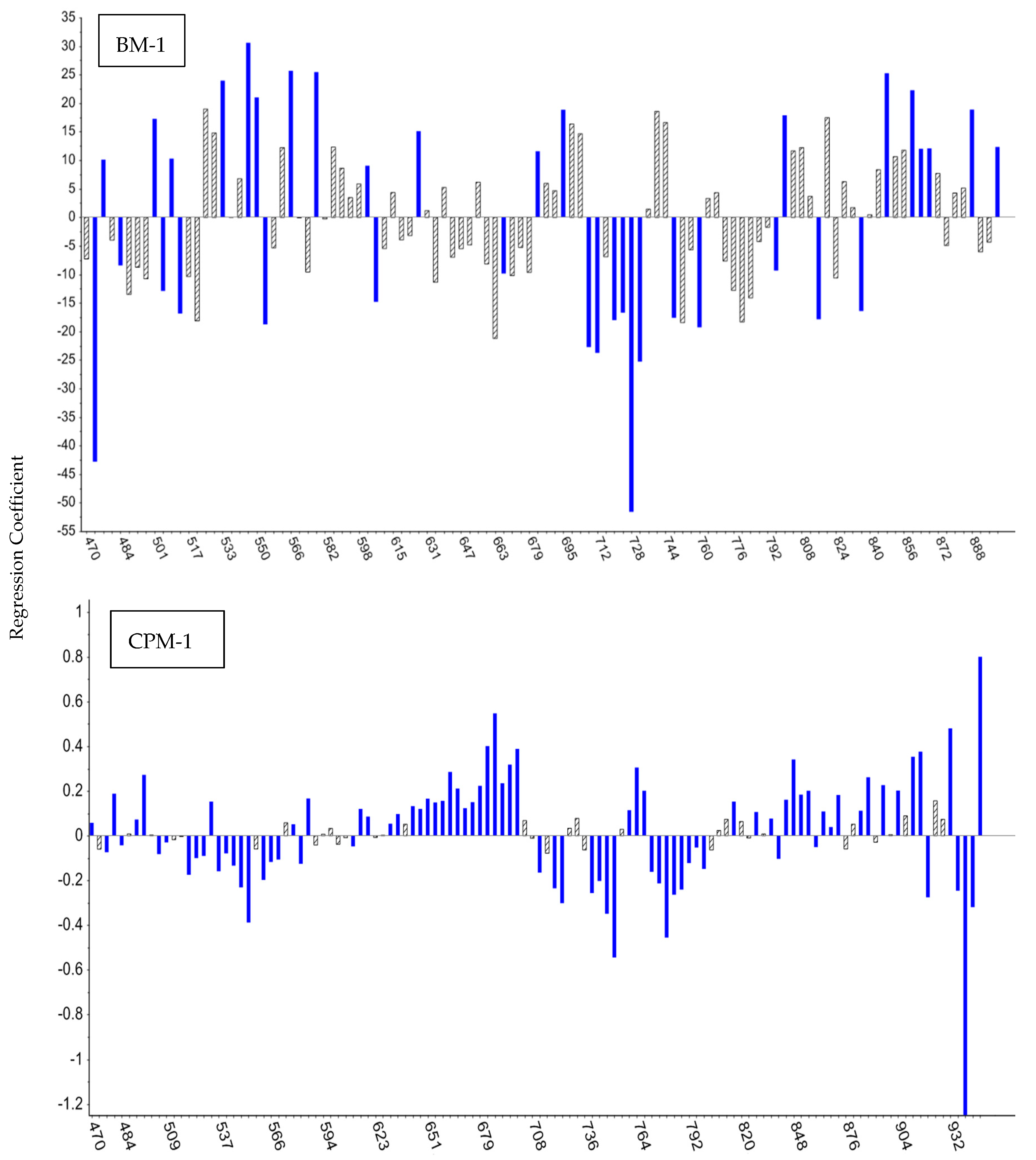
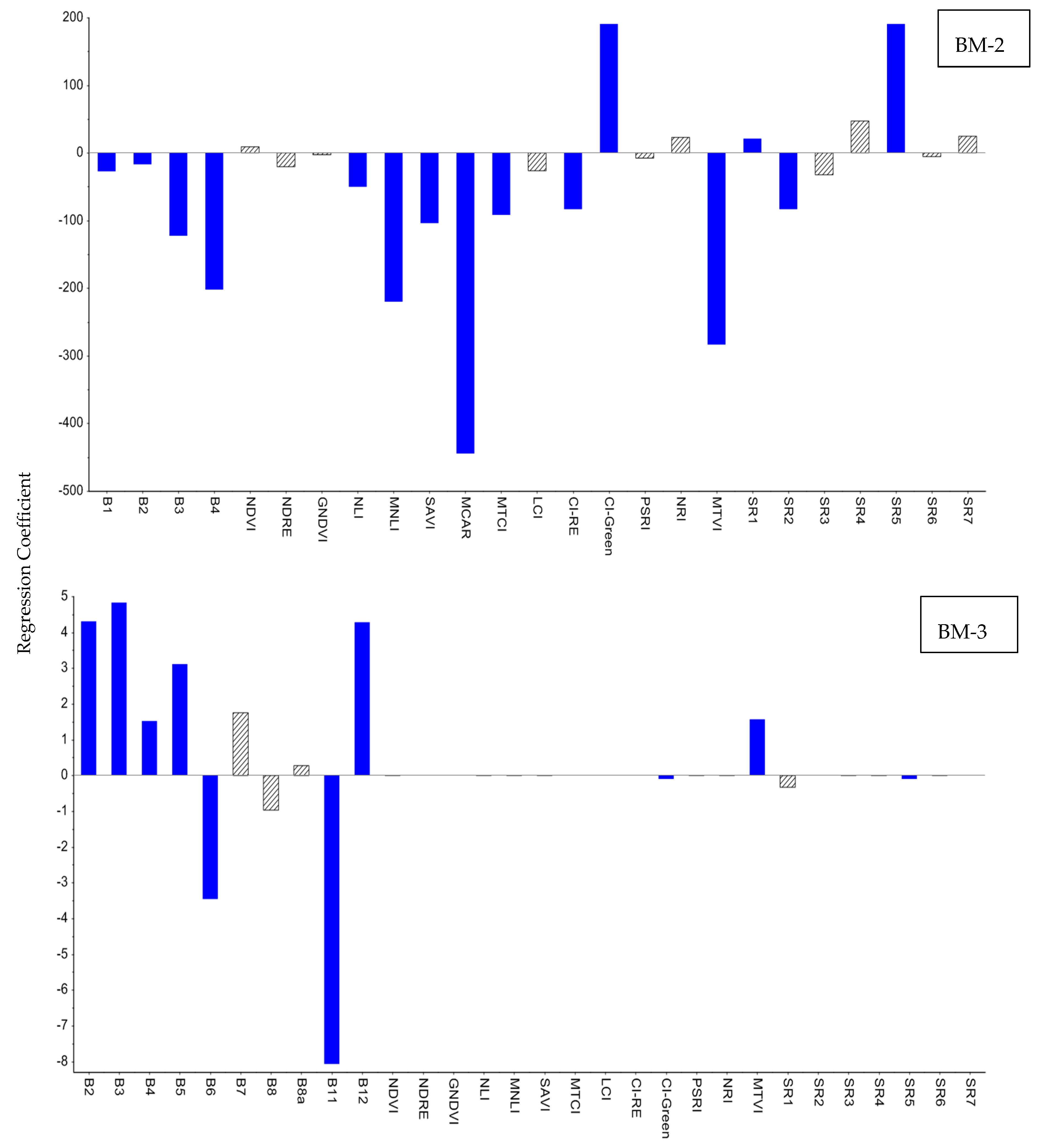
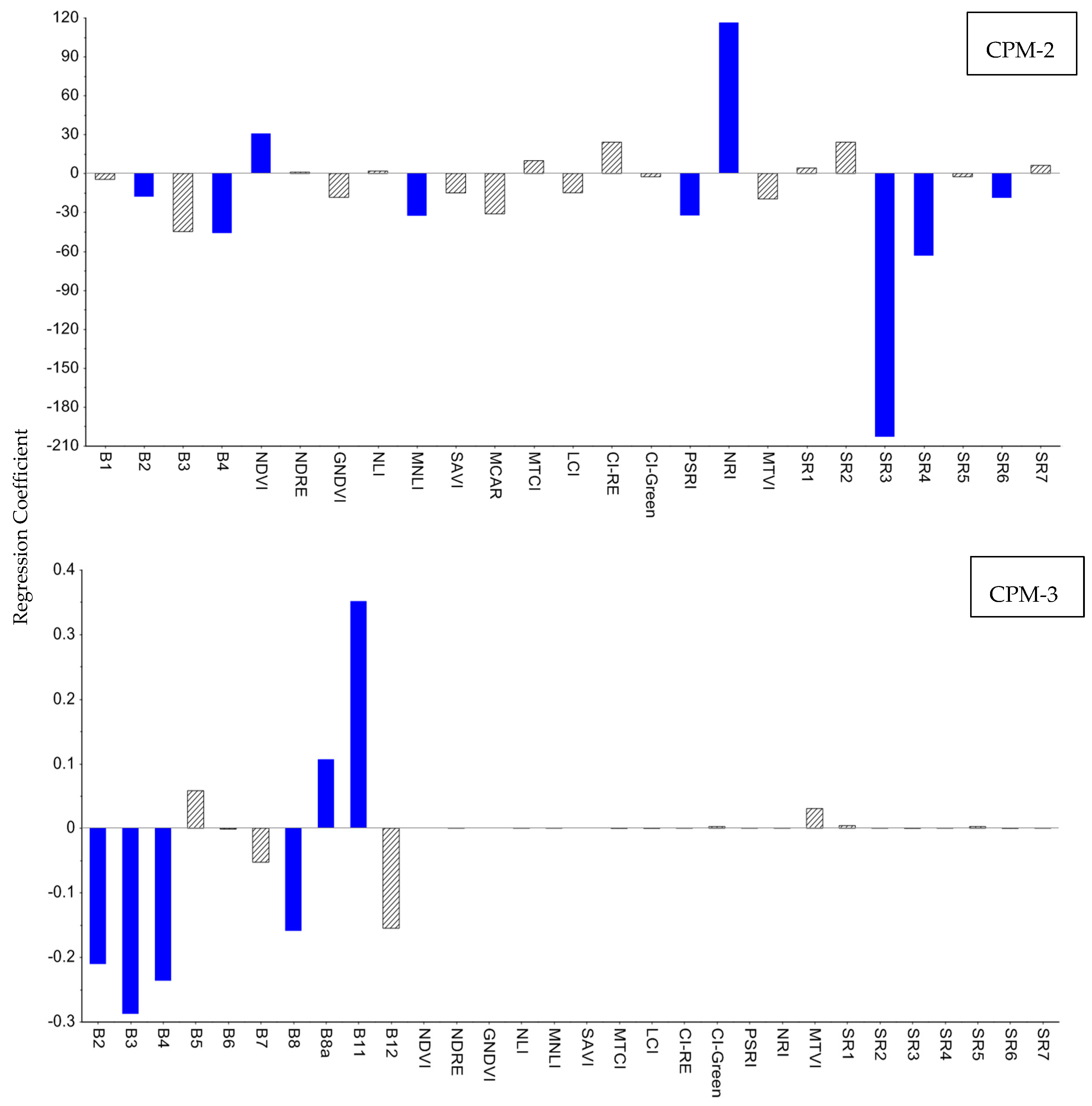
Eight, four, and five latent variables were identified as the proper number of factors for predicting grass BM using HSI, MSI-UAV, and MSI-Sentinel-2 datasets, respectively (Table 5). Similarly, five, five, and eight latent factors were identified for PLSR modelling of grass CP using HSI, MSI-UAV, and MSI-Sentinel-2 datasets, respectively (Table 6). The diagrams of prediction residual sum of squares versus the number of latent variables are displayed in Figure S1 (Supplementary Materials). These diagrams were used to determine the appropriate number of latent variables for producing PLSR models [5,66]. Important wavelengths for BM and CP predictions based on the Martens’ uncertainty test are presented in Figure 4. The significant regression coefficients of wavelengths (Figure 4, p-value < 0.001) are highlighted in blue. Wavelengths of 728 nm, 546 nm, and 472 nm had the maximum coefficients and had a greater impact on BM prediction. For the CP prediction, wavelengths of 940 nm > 948 nm > 688 nm > 752 nm had the maximum impact on the PLSR model. The highest coefficient for CP prediction was within the NIR range, while the red-edge range had the highest coefficient for BM perdition. Figure 5 demonstrates the regression coefficients of bands and spectral indices used for BM prediction using MSI-UAV and MSI-Sentinel 2. Of the 25 bands and indices, MCAR, MTVI, MNLI, band 4, CI-green, and SR5 had a high impact on BM prediction for MSI-UAV. Of the 35 Sentinel bands and indices, band 11, band 12, band 3, band 2, band 6, and band 5 had a greater influence on BM prediction for MSI-Sentinel-2. The significant regression coefficients of bands and spectral indices for predicting CP using MSI-UAV and MSI- Sentinel-2 were presented in Figure 6. The SR3 and NRI had the largest regression coefficients of the PLSR model for MSI-UAV. In addition, the highest regression coefficients for the PLSR model of MSI-Sentinel-2 belonged to band 11 and band 3.
The results of the PLSR models (summarized in Table 5 and Table 6) indicated that HSI had a better prediction for grass BM and CP than MSI (both UAV and Sentinel-2). An overall excellent accuracy was obtained for the HSI models (RPD > 2.5 and R2 = 0.82, validation model) and good accuracy for MSI-UAV models (RPD > 2 and R2 ≥ 0.77). While grass BM was predicted with a good accuracy using MSI-Sentinel-2, a moderate accuracy was obtained for CP prediction using Sentinel-2 images. The higher accuracy of the HSI models was noted consistently by R2, RMSEP, and RPD. The R2 of the HSI model for BM prediction was 13% higher than that of the MSI-UAV model (Table 5, validation set) and 7% higher than that of the MSI-Sentinel-2 model (Table 5, validation set). The RMSEP of the HSI model for predicting BM was also 17.4% lower than that of MSI-UAV model and 3.75 fold lower compared to the MSI-Sentinel-2 model. Specifically, 55% and 50% increases for RPD were also observed for the HSI model compared to the MSI-UAV and MSI-Sentinel-2, respectively, for prediction of BM. Although a slightly lower R2 (Table 5, 5% decrease) was noted for MSI-UAV compared to MSI-Sentinel-2, a 2.79 fold reduction in the RMSEP of the MSI-UAV model and a five percent increase for the RPD of MSI-UAV model compared to the MSI-Sentinel-2 indicated the higher accuracy of the PLSR model developed using an UAV than Sentinel-2 imagery for predicting grass BM. The better efficiency of the PLSR model for estimating CP using HSI data was also noted by 6.5% and 32% increases in R2, and 1.2% and 58% rises in RPD compared to MSI-UAV and MSI-Sentinel-2, respectively.
3.2. Predicting GQ Indicators Using MLR
The statistical parameters (RPD, R2, and RMSEP) used for assessing the accuracy of MLR models are presented in Table 7 and Table 8. Wavelengths of 473 nm, 481 nm, 675 nm, 687 nm, 909 nm, 913 nm, 927 nm, and 945 nm were identified as the important wavelengths and SR2 as the significant index through stepwise MLR approach for predicting BM using HSI. Wavelengths of 452 nm, 464 nm, 470 nm, 476 nm, 489 nm, MCAR, PSRI, SR1, and SR7 were also used for predicting CP using HSI. An excellent prediction was obtained for both BM and CP using HSI data (RPD > 2.5 and R2 > 0.80). The red-edge band (band 3) and a ratio of NIR and green bands (SR5) were found as important spectral data for BM prediction using stepwise MLR of the MSI-UAV. Band 2, band 8, band 11, band 12, GNDVI, and BRI were also identified as significant for BM prediction using MSI-Sentinel-2. To predict the CP through stepwise MLR, band 2, MCAR, and SR3 were identified as important via MSI-UAV, where band 6, band 11, band 8a, GNDVI, and LCI were determined as significant bands and indices via MSI-Sentinel-2. The stepwise MLR models of the selected spectral bands and indices suggested a moderate prediction of BM using both MSI datasets (Table 7, RPD ≥ 1.92, R2 ≥ 0.76). While the CP was estimated with good accuracy using MSI-UAV, the accuracy of the models for CP prediction was poor using MSI-Sentinel-2 (Table 8, R2 < 0.6, RPD = 1.39).
3.3. Evaluating Spectral Models
The comparison of measured and estimated values of BM and CP with a 1:1 line (Figures S2 and S3, Supplementary Materials) indicated an underestimation for high values and overestimation for low values of BM and CP for all prediction models. The paired t-test between measured and estimated BM and CP indicated no significant difference for all spectral datasets (Table 9 and Table 10). The variance comparison based on the Pitman–Morgan test revealed that the variance of estimated BM using HSI was not significantly different from that of measured BM for both PLSR and MLR models (Table 9). The variance of predicted BM using MSI (UAV and Sentinel-2) was statistically different from the measured values for both PLSR and MLR models. Regarding the prediction models of CP, the variance of measured and estimated values was not significantly different for PLSR and MLR models generated using HSI and MSI-UAV (Table 10). The variance of estimated CP calculated using MSI-Sentinel-2 was different (p-value < 0.05) from that of measured CP for both PLSR and MLR models.
The BM-1 and BM-4 (Figure 3) generated based on HSI had an excellent accuracy (Table 5, RPD > 2.5 and R2 > 0.8) which was also confirmed by paired mean and variance comparisons (Table 9). The models developed using both MSI-UAV and MSI-Sentinel-2 using PLSR (Figure 3, BM-1 and BM-2) were also reliable for predicting BM with good accuracy (2 < RPD < 2.5 and R2 > 0.7). The MLR models developed using MSI-UAV and MSI-Sentinel-2 had moderate accuracy for BM prediction (Figure 3, BM-5 and BM-6). The best prediction accuracy was obtained for BM-1, followed by BM-4 > BM-2 > BM-3 (Figure 3). Considering the CP models, excellent accuracy was obtained for CPM-1 and CPM-2 (Figure 3) calculated using HSI (Table 6, RPD > 2.5 and R2 > 0.8), and good accuracy was noted for CPM-2 and CPM-5 developed using MSI-UAV. Poor and moderate accuracy was also acquired using MSI-Sentinel-2 for predicting CP (Table 6 and Table 8).
The swath width of the hyperspectral imager was 0.3 m and the alignment of the images captured by the BaySpec imager was complicated over all 64 plots. Thus, in this research, the HSI data were recorded only over 16 plots (1D to 16D, Figure 2, red boundary). Since the hyperspectral images were only captured over 16 plots at each date, they did not have complete coverage over the plots. Therefore, BM-2 and BM-3, which also had good accuracy, were used to map BM using UAV (Figure S4, Supplementary Materials) and Sentinel-2 images (Figure S5, Supplementary Materials), respectively. The MSI-Sentinel 2 could not predict grass CP appropriately. Thus, the CP was mapped only using the MSI-UAV over 64 plots (Figure S6, Supplementary Materials)
4. Discussion
Different levels of grass BM and CP were studied by applying different levels of nitrogen fertilization in the study area (Table 1). The measured BM and CP (Table 4) were within the range usually reported for Irish grassland [34,67,68,69]. For accurate grass BM and CP modelling, the MSI-UAV datasets and the HSI data were transformed to surface reflectance images. The Sentinel-2 images were downloaded as “Level 2A Products” and were atmospherically corrected. In agreement with Edirisinghe et al. [70], the current study confirmed that surface reflectance correction was a mandatory pre-processing step for modelling GQ indicators, especially for satellite data captured over Ireland. The concurrence of available and cloud-free satellite data with field sampling is a major issue in the development of spectral models for pasture assessment using satellite data (MSI-Sentinel-2 in this study). A reliable satellite model can be computed when field sampling is carried out on the day of the satellite overpass. For an accurate prediction of grass indicators, the time gap between field sampling and the satellite overpass must be less than one week [70].
4.1. PLSR Prediction of GQ Indicators
Identifying the significant wavelengths using HSI emphasized the importance of red-edge > green > red > NIR region for predicting BM (Figure 4, BM-1), and the importance of NIR > red > red-edge > green for estimating CP (Figure 4, CPM-1). The identified wavelengths have been reported as important for spectral prediction of vegetation indicators [9,71]. Consistent with our finding, Clifton et al. [72] indicated the importance of the NIR and red range of the spectrum for accurate prediction of GQ indicators. A strong relationship between visible and NIR spectra and forage protein content was reported using hyperspectral remote sensing [6,73]. Higher nitrogen uptake by grass, which leads to increased chlorophyll content and grass growth, reduces the reflectance of visible spectra particularly in the red and green range of the spectrum [74]. The increased reflectance of NIR and red-edge spectra is also associated with the improvement of CP content and grass BM [37]. The importance of these wavelength ranges was also confirmed by identifying the most effective spectral indices for PLSR prediction of BM and CP using MSI-UAV. The MCAR and MTVI had the largest regression coefficient for spectral modelling of BM (Figure 5, BM2). The MCAR index is a combination of red-edge, green, and red bands, and the index of MTVI is an integration of green, red, and NIR bands of the Sequoia sensor (Figure 3). The greatest regression coefficients for PLSR prediction of CP were noted for NRI and SR3 (Figure 6, CPM-2). These indices were an integration of NIR, red, and green bands. Spectral indices, which are a combination of two or more bands, are usually more effective than a single spectral band for estimating plant biochemical parameters [75]. The ability of spectral indices to reduce the effect of background noise and enhance the robustness of biomass prediction models has been documented in the literature [23,24].
Band 11, centered at 1610 nm, and band 3, centered at 560 nm, had the maximum impact on the predictability of BM using Sentinel-2 images. Clevers and Gitelson [23] reported the importance of red-edge bands of Sentinel-2 (bands 5 and 6) for evaluating grass attributes. Although a reasonable level of accuracy was not obtained for predicting CP using MSI-Sentinel-2, band 11 and band 3 did have the maximum impact on spectral modelling of CP (Figure 6, CPM-3). Lugassi et al. [37] found band 3, band 4, band 8a, and band 12 as the most useful bands of Sentinel 2 for estimating protein content. The PLSR technique could reliably be used for spectral prediction of BM with an excellent accuracy using HSI and a good accuracy using UAV and Sentinel images. This technique is also successful for predicting grass CP, resulting in excellent accuracy using HSI data and a reasonable level of accuracy using UAV data. The PLSR was unable to model CP using Sentinel-2 images.
4.2. MLR Prediction of Grass CP and BM
While the MLR technique could predict grass BM and CP using HSI with a high degree of accuracy, it was not able to predict GQ indicators accurately using both MSI-UAV and MSI-Sentinel-2 (Table 7 and Table 8). The moderate and poor accuracies were noted using the MSI datasets. The most important spectra identified based on the HSI using stepwise MLR were the bands centered at 945 nm, 927 nm, 913 nm, 909 nm, 687 nm, 675 nm, 481 nm, and 473 nm for BM estimation and the bands centered at 489 nm, 476 nm, 470 nm, 464 nm, and 452 nm for CP prediction. Starks et al. [76] reported the importance of spectral bands centered at 915 nm, 865 nm, 765 nm, 755 nm, 725 nm, 605 nm, and 485 nm for predicting grass CP and fiber content. Wavelengths of 700 nm, 725 nm, 760 nm, and 775 nm were also reported as significant for predicting CP by Kawamura et al. [77]. A higher nitrogen content applied to the soil leads to a greater nitrogen concentration in plant tissues and rapid growth, which enhances grass BM and CP [78]. The NIR and red-edge wavelengths have been reported as sensitive spectral ranges to detect changes in plant growth [9]. Band 11 and band 12 of Sentinel-2 images (Short wave infrared bands) were also found important for MLR prediction of BM and CP (Table 7 and Table 8). Gong et al. [32] found that short-wave infrared (1300–2500 nm) regions could be more efficient than visible regions to predict forage CP and nitrogen concentration. The absorbance spectra at 2060 nm, 2130 nm, 2180 nm, and 2240 nm are associated with N–H and C–H bonds of protein [79,80]. An accurate estimation of forage attributes was also reported using the SWIR region of the spectrum by Pullanagari et al. [81] and Lugassi et al. [37]. Due to the low accuracy of models developed using MSI-Sentinel-2 and the spectral range of HSI images (Table 2, 450–950 nm), the efficiency of SWIR for predicting CP could not be evaluated in this study. The MLR technique could also be reliably used for evaluating GQ indicators using the HSI dataset, but it was not efficient enough to predict BM and CP using the MSI datasets (Sequoia and Sentinel-2 images).
4.3. Comparing the Predictability of Spectral Models
The use of different modelling approaches could result in different accuracies regardless of the type of spectral data [82]. The PLSR has been widely used for spectral prediction tasks [83,84]. The MLR has also been employed by several studies as a robust technique for spectral estimation of grass attributes (e.g., [85,86]). Therefore, these two techniques were deployed to estimate grass BM and CP. While some researchers reported the superiority of non-linear and intelligent approaches to linear techniques (e.g., [28,82]), PLSR and MLR showed a good efficiency for assessing GQ in this study. These techniques are relatively easy to understand and simpler than more automated machine learning approaches. Igne et al. [87] indicated that spectral models were sensitive to the complexity of the modelling approach. They concluded that the PLSR and locally weighted regression were simpler models to implement and compute compared to support vector machine regression for quantitative spectral analysis. Good efficiency of PLSR and MLR for modelling BM and CP indicated that a linear relationship might exist between grass spectral data and GQ parameters. These simple techniques also have the potential to be used for modelling other GQ indicators under grassland management systems in Ireland. Overall, 12 spectral models were developed, six models for BM prediction (Figure 3, BM-1 to BM-6) and six models for CP estimation (CPM-1 to CPM-6). The accuracy of MLR models was lower (Table 7 and Table 8) than PLSR models (Table 5 and Table 6). The PLSR technique could offer a better estimation of BM and CP, especially when it was performed on higher-resolution spectral data (HSI model). The prediction efficiency of PLSR using greater spectral resolution was also confirmed by Askari et al. [57]. The higher spectral and spatial resolution of HSI than that of the MSI-UAV and MSI-Sentinel-2 could be the reason for more accurate prediction of HSI [88]. The proximity to ground surface for the HSI compared to the MSI-UAV and MSI-Sentinel-2 could result in higher quality data and could be another reason for the greater accuracy of the HSI model. While the HSI method showed a better performance and efficiency, the high cost (typically €40,000 to €100,000) is the main issue regarding the use of the new generation hyperspectral cameras [89]. The high cost of the HSI was also mentioned by Mansour et al. [90] as an important limitation for local scale assessment of rangeland biomass in Africa. Real-time evaluation of grassland management systems in Ireland needs a low-cost, rapid, and accurate technique for a timely assessment of GQ [91]. An accurate prediction of grass BM can still be acquired using freely available MSI-Sentinel-2 data (Table 5) and cheaper multispectral sensors such as the Sequoia (MSI-UAV). The CP quality metric can also be predicted with a reasonable level of accuracy using multispectral imagery conducted by a UAV.
4.4. The Efficiency of Remote Sensing for Assessing GQ
The accuracy of the models (Table 5, Table 6, Table 7 and Table 8) and the paired analyses (Table 9 and Table 10) resulting from this study demonstrated that the spectral prediction and spatial monitoring of grass BM and CP in Ireland are possible using remote sensing techniques. These techniques can be used for direct assessment of GQ as an alternative to routine approaches. Laboratory-based methods for assessing GQ are time-consuming, costly, and labor-intensive for collecting and analyzing samples. On the other hand, using field spectroscopy techniques, which usually provide point spectral data, are more complicated and time consuming than using UAV and satellite imagery systems especially over a large scale [15]. Remote sensing imagery can provide rapid tools for monitoring the impact of management systems on GQ under temperate European grassland. The BM and CP maps (Figures S4 and S6; Supplementary Materials) indicated a descending trend from June to September in 2017, which was in agreement with laboratory measurements and the grass growth curve of Moorepark Research Centre in 2017 presented by the Agriculture and Food Development Authority in Ireland [92]. Furthermore, the impact of the drought period during 2018 in Ireland was also detectable by comparing the UAV images captured on 21 April 2018 and 11 July 2018 (Figures S4 and S6; Supplementary Materials). These results revealed that a near real-time information for on-the-go management of grassland in Ireland can be provided using the models developed in the current study. The spectral prediction of grass BM and CP using remote sensing techniques has very real potential for monitoring the sustainability of grass production sectors. Multi-temporal remote sensing images can be used for monitoring the changes in grass BM and CP during critical time periods and for assessing the effects of longer-term management operations on the quality of forage. The current study did not address the effects of different plant species and their within-field variabilities on the accuracy of models. Variable grass species could be explored in future studies.
5. Conclusions
With regard to the research objectives, the results indicated that:
- (a)
- The HSI technique yielded better prediction of grass BM and CP than MSI techniques. In this regard, excellent accuracy was obtained using HSI and good accuracy was acquired using both MSI-UAV and MSI-Sentinel-2 for predicting BM and using MSI-UAV for predicting CP.
- (b)
- Based on the HSI dataset, the red-edge range was identified as the most effective wavelength range for predicting grass BM, while the NIR range had the greatest influence on the spectral predictability of grass CP. A combination of red-edge, red and green bands (MCAR) was identified as the most useful index for estimating BM using MSI-UAV, and a ration of red and green bands (SR3) had the maximum impact on the prediction of CP using Sequoia images. Band 11 centred at 1610 nm was found to be the most important band for modelling GQ indicators using Sentinel-2 images.
- (c)
- Both the PLSR and MLR techniques yielded accurate models for prediction of BM and CP. The PLSR yielded better model outputs, though the results from both techniques were sufficiently robust to be used.
Surface reflectance transformation was found to be a mandatory atmospheric pre-processing correction step for predicting grass attributes. While the high cost is the main limitation of hyperspectral sensors, accurate quantification of grass indicators can be obtained using cheaper multispectral Sequoia sensors and freely available multispectral Sentinel-2 data. Both the HSI and MSI can be utilized as a rapid, reliable, and reproducible technique for near real-time quantitative assessment of GQ under intensive grassland management systems in the temperate European climate zone. Finally, within-filed variability of GQ can be accurately mapped and monitored using UAV and satellite remote sensing techniques.
Supplementary Materials
As part of this article, six figures are provided and mentioned in the manuscript as supplementary materials https://0-www-mdpi-com.brum.beds.ac.uk/2072-4292/11/15/1835/s1. Figure S1: Identification of the optimal number of latent variables used for biomass models (BM-1 to BM-3) and crude protein models (CPM-1 to CPM-3) developed using PLSR. Figure S2: Scatter plots of predicted BM versus actual BM. Figure S3: Scatter plots of predicted CP versus actual CP. Figure S4: Biomass maps predicted using MSI-UAV images (BM-2) captured on 12 June 2017 (A), 21 August 2017, (B) 18 September 2017 (C) from trial plots and 21 April 2018 (D) and 11 July 2018 (E) from Paddocks. Figure S5: Biomass (Kg DM ha−1) maps predicted using MSI-Sentinel-2 images (BM-3) on 21 April 2018 (D) and 16 May 2018 (E) from paddocks. Figure S6: Crude protein (g/Kg DM) maps predicted using MSI-UAV images (CMP-2) captured on 12 June 2017 (A), 21 August 2017, (B) 18 September 2017 (C) from trial plots and 21 April 2018 (D) and 11 July 2018 (E) from paddocks.
Author Contributions
Conceptualization, M.S.A. and T.M; methodology, M.S.A.; software, M.S.A.; validation, M.S.A.; formal analysis, M.S.A.; grass sampling and laboratory analysis, D.J.M.; investigation, M.S.A.; resources, M.S.A. and T.M.; data curation, M.S.A. and A.M.; writing—original draft preparation, M.S.A., review and editing, T.M. and M.S.A; visualization, M.S.A., T.M., and A.M.; supervision, M.S.A. and T.M.; funding acquisition, T.M.
Funding
This research was funded by the Department of Agriculture, Food, and the Marine, Ireland, under the ICT-Agri ERA-Net Precision Agriculture Call, Project ID 30070. ![Remotesensing 11 01835 i001]()

Conflicts of Interest
The authors declare no conflict of interest.
References
- Price, K.; Crooks, T.J.; Martinko, E.A. Grasslands across time and scale: A remote sensing perspective. Photogramm. Eng. Remote Sens. 2001, 67, 414–420. [Google Scholar]
- Hollberg, J.; Schellberg, J. Distinguishing Intensity Levels of Grassland Fertilization Using Vegetation Indices. Remote Sens. 2017, 9, 81. [Google Scholar] [CrossRef]
- Askari, M.S.; Holden, N.M. Indices for quantitative evaluation of soil quality under grassland management. Geoderma 2014, 230–231, 131–142. [Google Scholar] [CrossRef]
- Askari, M.S.; Cui, J.; Holden, N.M. The visual evaluation of soil structure under arable management. Soil Tillage Res. 2013, 134, 1–10. [Google Scholar] [CrossRef]
- Askari, M.S.; O’Rourke, S.M.; Holden, N.M. Evaluation of soil quality for agricultural production using visible–near-infrared spectroscopy. Geoderma 2015, 243–244, 80–91. [Google Scholar] [CrossRef]
- Ramoelo, A.; Cho, M.A.; Mathieu, R.; Madonsela, S.; van de Kerchove, R.; Kaszta, Z.; Wolff, E. Monitoring grass nutrients and biomass as indicators of rangeland quality and quantity using random forest modelling and WorldView-2 data. Int. J. Appl. Earth Obs. Geoinf. 2015, 43, 43–54. [Google Scholar] [CrossRef]
- Tudsri, S.; Jorgensen, S.; Riddach, P.; Pookpakdi, A. Effect of cutting height and dry season closing date on yield and quality of five napier grass cultivars in Thailand. Trop. Grassl. 2002, 36, 248–252. [Google Scholar]
- Skidmore, A.K.; Ferwerda, J.G.; Mutanga, O.; Van Wieren, S.E.; Peel, M.; Grant, R.C.; Prins, H.H.T.; Balcik, F.B.; Venus, V. Forage quality of savannas—Simultaneously mapping foliar protein and polyphenols for trees and grass using hyperspectral imagery. Remote Sens. Environ. 2010, 114, 64–72. [Google Scholar] [CrossRef]
- Sibanda, M.; Mutanga, O.; Rouget, M. Examining the potential of Sentinel-2 MSI spectral resolution in quantifying above ground biomass across different fertilizer treatments. ISPRS J. Photogramm. Remote Sens. 2015, 110, 55–65. [Google Scholar] [CrossRef]
- Schut, A.G.T.; Ketelaars, J.J.M.H.; Meuleman, J.; Kornet, J.G.; Lokhorst, C. AE—Automation and Emerging Technologies: Novel Imaging Spectroscopy for Grass Sward Characterization. Biosyst. Eng. 2002, 82, 131–141. [Google Scholar] [CrossRef]
- Pullanagari, R.R.; Yule, I.J.; Tuohy, M.P.; Hedley, M.J.; Dynes, R.A.; King, W.M. In-field hyperspectral proximal sensing for estimating quality parameters of mixed pasture. Precis. Agric. 2012, 13, 351–369. [Google Scholar] [CrossRef]
- Safari, H.; Fricke, T.; Wachendorf, M. Determination of fibre and protein content in heterogeneous pastures using field spectroscopy and ultrasonic sward height measurements. Comput. Electron. Agric. 2016, 123, 256–263. [Google Scholar] [CrossRef]
- Zhao, D.; Starks, P.J.; Brown, M.A.; Phillips, W.A.; Coleman, S.W. Assessment of forage biomass and quality parameters of bermudagrass using proximal sensing of pasture canopy reflectance. Grassl. Sci. 2007, 53, 39–49. [Google Scholar] [CrossRef]
- Schweiger, A.K.; Risch, A.C.; Damm, A.; Kneubühler, M.; Haller, R.; Schaepman, M.E.; Schütz, M. Using imaging spectroscopy to predict above-ground plant biomass in alpine grasslands grazed by large ungulates. J. Veg. Sci. 2015, 26, 175–190. [Google Scholar] [CrossRef]
- Bendig, J.; Yu, K.; Aasen, H.; Bolten, A.; Bennertz, S.; Broscheit, J.; Gnyp, M.L.; Bareth, G. Combining UAV-based plant height from crop surface models, visible, and near infrared vegetation indices for biomass monitoring in barley. Int. J. Appl. Earth Obs. Geoinf. 2015, 39, 79–87. [Google Scholar] [CrossRef]
- Zhang, W.; Yang, X.; Manlike, A.; Jin, Y.; Zheng, F.; Guo, J.; Shen, G.; Zhang, Y.; Xu, B. Comparative study of remote sensing estimation methods for grassland fractional vegetation coverage—A grassland case study performed in Ili prefecture, Xinjiang, China. Int. J. Remote Sens. 2018, 1–16. [Google Scholar] [CrossRef]
- Wachendorf, M.; Fricke, T.; Möckel, T. Remote sensing as a tool to assess botanical composition, structure, quantity and quality of temperate grasslands. Grass Forage Sci. 2018, 73, 1–14. [Google Scholar] [CrossRef]
- Wu, H.; Li, Z.-L. Scale issues in remote sensing: a review on analysis, processing and modeling. Sensors (Basel, Switzerland) 2009, 9, 1768–1793. [Google Scholar] [CrossRef]
- Yang, J.; Gong, P.; Fu, R.; Zhang, M.; Chen, J.; Liang, S.; Xu, B.; Shi, J.; Dickinson, R. The role of satellite remote sensing in climate change studies. Nat. Clim. Change 2013, 3, 875. [Google Scholar] [CrossRef]
- Jia, Z.L.; Lu, X.P.; Zheng, F.J.; Zang, W.Q.; Liu, Q.C. Research on atmospheric correction and surface reflectance inversion of UAV (Unmanned Aerial Vehicle) remote sensing data. Appl. Mech. Mater. 2013, 427–429, 1485–1488. [Google Scholar] [CrossRef]
- Fava, F.; Colombo, R.; Bocchi, S.; Meroni, M.; Sitzia, M.; Fois, N.; Zucca, C. Identification of hyperspectral vegetation indices for Mediterranean pasture characterization. Int. J. Appl. Earth Obs. Geoinf. 2009, 11, 233–243. [Google Scholar] [CrossRef]
- Lugassi, R.; Chudnovsky, A.; Zaady, E.; Dvash, L.; Goldshleger, N. Estimating Pasture Quality of Fresh Vegetation Based on Spectral Slope of Mixed Data of Dry and Fresh Vegetation—Method Development. Remote Sens. 2015, 7, 8045. [Google Scholar] [CrossRef]
- Clevers, J.G.P.W.; Gitelson, A.A. Remote estimation of crop and grass chlorophyll and nitrogen content using red-edge bands on Sentinel-2 and -3. Int. J. Appl. Earth Obs. Geoinf. 2013, 23, 344–351. [Google Scholar] [CrossRef]
- Helman, D.; Mussery, A.; Lensky, I.M.; Leu, S. Detecting changes in biomass productivity in a different land management regimes in drylands using satellite-derived vegetation index. Soil Use Manag. 2014, 30, 32–39. [Google Scholar] [CrossRef]
- Yiran, G.A.B.; Kusimi, J.M.; Kufogbe, S.K. A synthesis of remote sensing and local knowledge approaches in land degradation assessment in the Bawku East District, Ghana. Int. J. Appl. Earth Obs. Geoinf. 2012, 14, 204–213. [Google Scholar] [CrossRef]
- Ali, I.; Cawkwell, F.; Dwyer, E.; Barrett, B.; Green, S. Satellite remote sensing of grasslands: From observation to management. J. Plant Ecol. 2016, 9, 649–671. [Google Scholar] [CrossRef]
- Numata, I.; Roberts, D.A.; Chadwick, O.A.; Schimel, J.P.; Galvão, L.S.; Soares, J.V. Evaluation of hyperspectral data for pasture estimate in the Brazilian Amazon using field and imaging spectrometers. Remote Sens. Environ. 2008, 112, 1569–1583. [Google Scholar] [CrossRef]
- Clevers, J.; Van der Heijden, G.; Verzakov, S.; Schaepman, M. Estimating grassland biomass using SVM band shaving of hyperspectral data. Photogramm. Eng. Remote Sens. 2007, 73, 1141–1148. [Google Scholar] [CrossRef]
- Gao, J. Quantification of grassland properties: how it can benefit from geoinformatic technologies? Int. J. Remote Sens. 2006, 27, 1351–1365. [Google Scholar] [CrossRef]
- Nordkvist, E.; Larsson, K. An approach to the use of multivariate analysis of near infrared spectroscopy (NIR) data from field-trials. Field Crops Res. 1994, 37, 33–38. [Google Scholar] [CrossRef]
- Cozzolino, D. Use of Infrared Spectroscopy for In-Field Measurement and Phenotyping of Plant Properties: Instrumentation, Data Analysis, and Examples. Appl. Spectrosc. Rev. 2014, 49, 564–584. [Google Scholar] [CrossRef]
- Gong, Z.; Kawamura, K.; Ishikawa, N.; Inaba, M.; Alateng, D. Estimation of herbage biomass and nutritive status using band depth features with partial least squares regression in Inner Mongolia grassland, China. Grassl. Sci. 2016, 62, 45–54. [Google Scholar] [CrossRef]
- Nouri, M.; Gomez, C.; Gorretta, N.; Roger, J.M. Clay content mapping from airborne hyperspectral Vis-NIR data by transferring a laboratory regression model. Geoderma 2017, 298, 54–66. [Google Scholar] [CrossRef]
- McEvoy, M.; O’Donovan, M.; Shalloo, L. Development and application of an economic ranking index for perennial ryegrass cultivars. J. Dairy Sci. 2011, 94, 1627–1639. [Google Scholar] [CrossRef] [PubMed]
- AOAC. Official Methods and Analysis, 15th ed.; Method 990-03; AOAC: Arlington, VA, USA, 1990. [Google Scholar]
- Kokaly, R.F. Investigating a Physical Basis for Spectroscopic Estimates of Leaf Nitrogen Concentration. Remote Sens. Environ. 2001, 75, 153–161. [Google Scholar] [CrossRef]
- Lugassi, R.; Zaady, E.; Goldshleger, N.; Shoshany, M.; Chudnovsky, A. Spatial and Temporal Monitoring of Pasture Ecological Quality: Sentinel-2-Based Estimation of Crude Protein and Neutral Detergent Fiber Contents. Remote Sens. 2019, 11, 799. [Google Scholar] [CrossRef]
- Rondeaux, G.; Steven, M.; Baret, F. Optimization of soil-adjusted vegetation indices. Remote Sens. Environ. 1996, 55, 95–107. [Google Scholar] [CrossRef]
- Haboudane, D.; Miller, J.R.; Pattey, E.; Zarco-Tejada, P.J.; Strachan, I.B. Hyperspectral vegetation indices and novel algorithms for predicting green LAI of crop canopies: Modeling and validation in the context of precision agriculture. Remote Sens. Environ. 2004, 90, 337–352. [Google Scholar] [CrossRef]
- Daughtry, C.S.T.; Walthall, C.L.; Kim, M.S.; de Colstoun, E.B.; McMurtrey, J.E. Estimating Corn Leaf Chlorophyll Concentration from Leaf and Canopy Reflectance. Remote Sens. Environ. 2000, 74, 229–239. [Google Scholar] [CrossRef]
- Dash, J.; Curran, P.J. The MERIS terrestrial chlorophyll index. Int. J. Remote Sens. 2004, 25, 5403–5413. [Google Scholar] [CrossRef]
- Schleicher, T.D.; Bausch, W.C.; Delgado, J.A.; Ayers, P.D. Evaluation and Refinement of the Nitrogen Reflectance Index (NRI) for Site-Specific Fertilizer Management; The American Society of Agricultural and Biological Engineers: St. Joseph, MI, USA, 2001. [Google Scholar]
- Gitelson, A.A.; Gritz, Y.; Merzlyak, M.N. Relationships between leaf chlorophyll content and spectral reflectance and algorithms for non-destructive chlorophyll assessment in higher plant leaves. J. Plant Physiol. 2003, 160, 271–282. [Google Scholar] [CrossRef]
- Hill, M.J. Vegetation index suites as indicators of vegetation state in grassland and savanna: An analysis with simulated Sentinel 2 data for a North American transect. Remote Sens. Environ. 2013, 137, 94–111. [Google Scholar] [CrossRef]
- Goel, N.S.; Qin, W. Influences of canopy architecture on relationships between various vegetation indices and LAI and Fpar: A computer simulation. Remote Sens. Rev. 1994, 10, 309–347. [Google Scholar] [CrossRef]
- Yang, Z.; Willis, P.; Mueller, R. Impact of band-ratio enhanced AWIFS image to crop classification accuracy. In Proceedings of the Pecora 17—The Future of Land Imaging, Denver, CO, USA, 18–20 November 2008. [Google Scholar]
- Ramoelo, A.; Skidmore, A.K.; Cho, M.A.; Schlerf, M.; Mathieu, R.; Heitkönig, I.M.A. Regional estimation of savanna grass nitrogen using the red-edge band of the spaceborne RapidEye sensor. Int. J. Appl. Earth Obs. Geoinform. 2012, 19, 151–162. [Google Scholar] [CrossRef]
- Sims, D.A.; Gamon, J.A. Relationships between leaf pigment content and spectral reflectance across a wide range of species, leaf structures and developmental stages. Remote Sens. Environ. 2002, 81, 337–354. [Google Scholar] [CrossRef]
- Smith, R.; Adams, J.; Stephens, D.; Hick, P. Forecasting wheat yield in a Mediterranean-type environment from the NOAA satellite. Aust. J. Agric. Res. 1995, 46, 113–125. [Google Scholar] [CrossRef]
- Lu, H.; Mack, J.; Yang, Y.; Shen, Z. Structural modification strategies for the rational design of red/NIR region BODIPYs. Chem. Soc. Rev. 2014, 43, 4778–4823. [Google Scholar] [CrossRef] [PubMed] [Green Version]
- De Sousa, C.; Souza, C.; Zanella, L.; De Carvalho, L. Analysis of Rapideye’s Red edge band for image segmentation and classification. In Proceedings of the 4th GEOBIA, Rio de Janeiro, Brazil, 7–9 May 2019; 2012; p. 58. [Google Scholar]
- Martens, H.; Martens, M. Modified Jack-knife estimation of parameter uncertainty in bilinear modelling by partial least squares regression (PLSR). Food Qual. Prefer. 2000, 11, 5–16. [Google Scholar] [CrossRef]
- Lee, H.W.; Bawn, A.; Yoon, S. Reproducibility, complementary measure of predictability for robustness improvement of multivariate calibration models via variable selections. Anal. Chim. Acta 2012, 757, 11–18. [Google Scholar] [CrossRef]
- Cheng, J.-H.; Jin, H.; Liu, Z. Developing a NIR multispectral imaging for prediction and visualization of peanut protein content using variable selection algorithms. Infrared Phys. Technol. 2018, 88, 92–96. [Google Scholar] [CrossRef]
- Andersen, C.M.; Bro, R. Variable selection in regression—A tutorial. J. Chemom. 2010, 24, 728–737. [Google Scholar] [CrossRef]
- Feilhauer, H.; Asner, G.P.; Martin, R.E. Multi-method ensemble selection of spectral bands related to leaf biochemistry. Remote Sens. Environ. 2015, 164, 57–65. [Google Scholar] [CrossRef]
- Askari, M.S.; O’Rourke, S.M.; Holden, N.M. A comparison of point and imaging visible-near infrared spectroscopyfor determining soil organic carbon. J. Near Infrared Spectrosc. 2018, 26, 133–146. [Google Scholar] [CrossRef]
- Yang, S.; Feng, Q.; Liang, T.; Liu, B.; Zhang, W.; Xie, H. Modeling grassland above-ground biomass based on artificial neural network and remote sensing in the Three-River Headwaters Region. Remote Sens. Environ. 2018, 204, 448–455. [Google Scholar] [CrossRef]
- Martínez Gila, D.M.; Cano Marchal, P.; Gómez Ortega, J.; Gámez García, J. Non-Invasive Methodology to Estimate Polyphenol Content in Extra Virgin Olive Oil Based on Stepwise Multilinear Regression. Sensors 2018, 18, 975. [Google Scholar] [CrossRef] [PubMed]
- Mahmoud, S.; Lotfi, A.; Langensiepen, C. User Activities Outliers Detection; Integration of Statistical and Computational Intelligence Techniques. Comput. Intell. 2016, 32, 49–71. [Google Scholar] [CrossRef]
- Williams, J.D.; Woodall, W.H.; Birch, J.B.; Sullivan, J.H. Distribution of Hotelling’s T2 Statistic Based on the Successive Differences Estimator. J. Qual. Technol. 2006, 38, 217–229. [Google Scholar] [CrossRef]
- Pitman, E.J.G. A Note on Normal Correlation. Biometrika 1939, 31, 9–12. [Google Scholar] [CrossRef]
- Morgan, W.A. A Test for the Significance of the Difference Between the Two Variances in a Sample From a Normal Bivariate Population. Biometrika 1939, 31, 13–19. [Google Scholar] [CrossRef]
- Muñoz-Montplet, C.; Marruecos, J.; Buxó, M.; Jurado-Bruggeman, D.; Romera-Martínez, I.; Bueno, M.; Vilanova, J.C. Dosimetric impact of Acuros XB dose-to-water and dose-to-medium reporting modes on VMAT planning for head and neck cancer. Phys. Med. 2018, 55, 107–115. [Google Scholar] [CrossRef]
- Viscarra-Rossel, R.A. Robust Modelling of Soil Diffuse Reflectance Spectra by “Bagging-Partial Least Squares Regression”. J. Near Infrared Spectrosc. 2007, 15, 39–47. [Google Scholar] [CrossRef]
- Geladi, P.; Kowalski, B.R. Partial least-squares regression: a tutorial. Anal. Chimi. Acta 1986, 185, 1–17. [Google Scholar] [CrossRef]
- McEniry, J.; Crosson, P.; Finneran, E.; McGee, M.; Keady, T.; O’Kiely, P. How much grassland biomass is available in Ireland in excess of livestock requirements? Irish J. Agric. Food Res. 2013, 67–80. [Google Scholar]
- Meehan, P.; Burke, B.; Doyle, D.; Barth, S.; Finnan, J. Exploring the potential of grass feedstock from marginal land in Ireland: Does marginal mean lower yield? Biomass Bioenerg. 2017, 107, 361–369. [Google Scholar] [CrossRef]
- Burns, G.A.; Gilliland, T.J.; Grogan, D.; Watson, S.; O’Kiely, P. Assessment of herbage yield and quality traits of perennial ryegrasses from a national variety evaluation scheme. J. Agric. Sci. 2012, 151, 331–346. [Google Scholar] [CrossRef]
- Edirisinghe, A.; Hill, M.J.; Donald, G.E.; Hyder, M. Quantitative mapping of pasture biomass using satellite imagery. Int. J. Remote Sens. 2011, 32, 2699–2724. [Google Scholar] [CrossRef]
- Ramoelo, A.; Skidmore, A.K.; Cho, M.A.; Mathieu, R.; Heitkönig, I.M.A.; Dudeni-Tlhone, N.; Schlerf, M.; Prins, H.H.T. Non-linear partial least square regression increases the estimation accuracy of grass nitrogen and phosphorus using in situ hyperspectral and environmental data. ISPRS J. Photogramm. Remote Sens. 2013, 82, 27–40. [Google Scholar] [CrossRef]
- Clifton, K.E.; Bradbury, J.W.; Vehrencanp, S.L. The fine-scale mapping of grassland protein densities. Grass Forage Sci. 1994, 49, 1–8. [Google Scholar] [CrossRef]
- Wang, Z.J.; Wang, J.H.; Liu, L.Y.; Huang, W.J.; Zhao, C.J.; Wang, C.Z. Prediction of grain protein content in winter wheat (Triticum aestivum L.) using plant pigment ratio (PPR). Field Crops Res. 2004, 90, 311–321. [Google Scholar] [CrossRef]
- Elarab, M.; Ticlavilca, A.M.; Torres-Rua, A.F.; Maslova, I.; McKee, M. Estimating chlorophyll with thermal and broadband multispectral high resolution imagery from an unmanned aerial system using relevance vector machines for precision agriculture. Int. J. Appl. Earth Obs. Geoinformat. 2015, 43, 32–42. [Google Scholar] [CrossRef] [Green Version]
- Bannari, A.; Morin, D.; Bonn, F.; Huete, A.R. A review of vegetation indices. Remote Sens. Rev. 1995, 13, 95–120. [Google Scholar] [CrossRef]
- Starks, P.J.; Zhao, D.; Phillips, W.A.; Coleman, S.W. Development of canopy reflectance algorithms for real-time prediction of bermudagrass pasture biomass and nutritive values. Crop Sci. 2006, 46, 927–934. [Google Scholar] [CrossRef]
- Kawamura, K.; Watanabe, N.; Sakanoue, S.; Inoue, Y. Estimating forage biomass and quality in a mixed sown pasture based on partial least squares regression with waveband selection. Grassl. Sci. 2008, 54, 131–145. [Google Scholar] [CrossRef]
- Bassegio, D.; Santos, R.F.; de Oliveira, E.; Wernecke, I.; Secco, D.; de Souza, S.N.M. Effect of nitrogen fertilization and cutting age on yield of tropical forage plants. Afr. J. Agric. Res. 2013, 8, 1427–1432. [Google Scholar]
- Card, D.H.; Peterson, D.L.; Matson, P.A.; Aber, J.D. Prediction of leaf chemistry by the use of visible and near infrared reflectance spectroscopy. Remote Sens. Environ. 1988, 26, 123–147. [Google Scholar] [CrossRef]
- Curran, P.J. Remote sensing of foliar chemistry. Remote Sens. Environ. 1989, 30, 271–278. [Google Scholar] [CrossRef]
- Pullanagari, R.R.; Yule, I.J.; Hedley, M.J.; Tuohy, M.P.; Dynes, R.A.; King, W.M. Multi-spectral radiometry to estimate pasture quality components. Precis. Agric. 2012, 13, 442–456. [Google Scholar] [CrossRef]
- Ali, I.; Cawkwell, F.; Dwyer, E.; Green, S. Modeling Managed Grassland Biomass Estimation by Using Multitemporal Remote Sensing Data—A Machine Learning Approach. IEEE J. Sel. Top. Appl. Earth Obs. Remote Sens. 2017, 10, 3254–3264. [Google Scholar] [CrossRef]
- Cho, M.A.; Skidmore, A.; Corsi, F.; van Wieren, S.E.; Sobhan, I. Estimation of green grass/herb biomass from airborne hyperspectral imagery using spectral indices and partial least squares regression. Int. J. Appl. Earth Obs. Geoinf. 2007, 9, 414–424. [Google Scholar] [CrossRef]
- Li, X.; Zhang, Y.; Bao, Y.; Luo, J.; Jin, X.; Xu, X.; Song, X.; Yang, G. Exploring the Best Hyperspectral Features for LAI Estimation Using Partial Least Squares Regression. Remote Sens. 2014, 6, 6221. [Google Scholar] [CrossRef]
- Park, R.S.; Gordon, F.J.; Agnew, R.E.; Barnes, R.J.; Steen, R.W.J. The use of Near Infrared Reflectance Spectroscopy on dried samples to predict biological parameters of grass silage. Anim. Feed Sci. Technol. 1997, 68, 235–246. [Google Scholar] [CrossRef]
- Cheng, J.-H.; Sun, D.-W.; Pu, H.-B.; Wang, Q.-J.; Chen, Y.-N. Suitability of hyperspectral imaging for rapid evaluation of thiobarbituric acid (TBA) value in grass carp (Ctenopharyngodon idella) fillet. Food Chem. 2015, 171, 258–265. [Google Scholar] [CrossRef] [PubMed]
- Igne, B.; Reeves, J.B.; McCarty, G.; Hively, W.D.; Lund, E.; Hurburgh, C.R. Evaluation of Spectral Pretreatments, Partial Least Squares, Least Squares Support Vector Machines and Locally Weighted Regression for Quantitative Spectroscopic Analysis of Soils. J. Near Infrared Spectrosc. 2010, 18, 167–176. [Google Scholar] [CrossRef] [Green Version]
- Abdel-Rahman, E.M.; Mutanga, O.; Odindi, J.; Adam, E.; Odindo, A.; Ismail, R. A comparison of partial least squares (PLS) and sparse PLS regressions for predicting yield of Swiss chard grown under different irrigation water sources using hyperspectral data. Comput. Electron. Agric. 2014, 106, 11–19. [Google Scholar] [CrossRef]
- Adjorlolo, C.; Mutanga, O.; Cho, M.A. Predicting C3 and C4 grass nutrient variability using in situ canopy reflectance and partial least squares regression. Int. J. Remote Sens. 2015, 36, 1743–1761. [Google Scholar] [CrossRef]
- Mansour, K.; Mutanga, O.; Everson, T. Remote sensing based indicators of vegetation species for assessing rangeland degradation: opportunities and challenges. Afr. J. Agric. Res. 2012, 7, 3261–3270. [Google Scholar]
- Hanrahan, L.; Geoghegan, A.; O’Donovan, M.; Griffith, V.; Ruelle, E.; Wallace, M.; Shalloo, L. PastureBase Ireland: A grassland decision support system and national database. Comput. Electron. Agric. 2017, 136, 193–201. [Google Scholar] [CrossRef]
- Teagasc. National Grass Growth Curve from Pasture Base Ireland. Available online: https://www.teagasc.ie/crops/grassland/pasturebase-ireland/grass-curve/ (accessed on 15 July 2019).
Figure 1.
Location of studied paddocks. The red boundary shows the paddocks studied in 2017 and the blue boundary illustrates the paddocks studied in 2018.
Figure 1.
Location of studied paddocks. The red boundary shows the paddocks studied in 2017 and the blue boundary illustrates the paddocks studied in 2018.

Figure 2.
Location of studied plots. The red boundary shows the plots used for the hyperspectral imagery (HSI) test and the black boundary shows the plots used for the multispectral imagery (MSI) test.
Figure 2.
Location of studied plots. The red boundary shows the plots used for the hyperspectral imagery (HSI) test and the black boundary shows the plots used for the multispectral imagery (MSI) test.

Figure 3.
The biomass models (BM) and crude protein models (CPM) calculated using partial least squares regression (PLSR) and stepwise multi-linear regression (MLR). HSI: hyperspectral imagery; MSI: multispectral imagery; Sat: Satellite; UAV: unmanned aircraft vehicle.
Figure 3.
The biomass models (BM) and crude protein models (CPM) calculated using partial least squares regression (PLSR) and stepwise multi-linear regression (MLR). HSI: hyperspectral imagery; MSI: multispectral imagery; Sat: Satellite; UAV: unmanned aircraft vehicle.

Figure 4.
Important wavelengths identified using the HSI dataset for predicting biomass (BM-1) and crude protein (CPM-1). Blue bars indicate significant wavelength with p < 0.05.
Figure 4.
Important wavelengths identified using the HSI dataset for predicting biomass (BM-1) and crude protein (CPM-1). Blue bars indicate significant wavelength with p < 0.05.

Figure 5.
Important bands and spectral indices identified using the MSI-UAV dataset (BM-2) and MSI- Sentinel-2 dataset (BM-3) for predicting biomass. Blue bars indicate significant bands and indices with p < 0.05.
Figure 5.
Important bands and spectral indices identified using the MSI-UAV dataset (BM-2) and MSI- Sentinel-2 dataset (BM-3) for predicting biomass. Blue bars indicate significant bands and indices with p < 0.05.

Figure 6.
Important bands and spectral indices identified using the MSI-UAV dataset (CMP-2) and MSI-Sentinel-2 dataset (CMP-3) for predicting CP. Blue bars indicate significant bands and indices with p < 0.05.
Figure 6.
Important bands and spectral indices identified using the MSI-UAV dataset (CMP-2) and MSI-Sentinel-2 dataset (CMP-3) for predicting CP. Blue bars indicate significant bands and indices with p < 0.05.


Table 1.
The amount of nitrogen applied to the studied plots and paddocks annually.
| Plots | Paddocks | ||||
|---|---|---|---|---|---|
| Plot ID | N (kg/ha) | 2017 | 2018 | ||
| Paddock ID | N (kg/ha) | Paddock ID | N (kg/ha) | ||
| 1 (A, B, C, D) | 0 | 2 (A, B, C, D, E, F) | 225 | 37 (A) | 150 |
| 2 (A, B, C, D) | 244 | 3 (B, C) | 250 | 37 (B) | 100 |
| 3 (A, B, C, D) | 0 | 4 (A, B, C) | 250 | 37 (C) | 250 |
| 4 (A, B, C, D) | 244 | 9 (A, B, C, D) | 225 | 38 (A) | 250 |
| 5 (A, B, C, D) | 480 | 10 (A, B, C, D, E, F) | 225 | 38 (B) | 100 |
| 6 (A, B, C, D) | 480 | 11 (A, B, C, D, E, F) | 250 | 38 (C) | 150 |
| 7 (A, B, C, D) | 119 | 12 (A, B) | 225 | ||
| 8 (A, B, C, D) | 119 | 20 (A, B, C) | 265 | ||
| 9 (A, B, C, D) | 0 | 21 (A, B, C) | 265 | ||
| 10 (A, B, C, D) | 480 | 42 (A, B, C) | 265 | ||
| 11 (A, B, C, D) | 480 | 43 (A, B, C) | 265 | ||
| 12 (A, B, C, D) | 244 | 44 (A, B, C) | 250 | ||
| 13 (A, B, C, D) | 119 | 45 (A, B, C) | 250 | ||
| 14 (A, B, C, D) | 244 | ||||
| 15 (A, B, C, D) | 119 | ||||
| 16 (A, B, C, D) | 0 | ||||
Table 2.
Characteristics of spectral datasets.
| Spectral Datasets | Operation Location | Sensor | Bands | Resolution | Wavelength Range |
|---|---|---|---|---|---|
| HIS 1 | 16 plots | BaySpec | 124 | 0.5 cm | 450 to 950 nm |
| MSI 2-UAV 3 | 64 plots | Sequoia | 4 | 2.86 and 11.29 cm | B1 (550 nm), B2 (660 nm), B3 (735 nm), B4 (790 nm) |
| 6 paddocks | |||||
| MSI-Sentinel-2 | 47 paddocks | Sentinel-2 | 10 | 10 and 20 m | B2 (490 nm), B3 (560 nm), B4 (665 nm), B5 (705 nm), B6 (740 nm), B7 (783 nm), B8 (842 nm), B8a (865 nm), B11 (1610 nm), B12 (2190 nm) |
| 6 paddocks |
1 HSI: hyperspectral imagery; 2 MSI: multispectral imagery; 3 UAV: unmanned aircraft vehicles.
Table 3.
Vegetation indices used for developing spectral models.
| Spectral Index | Equation | References |
|---|---|---|
| NDVI 1 | (NIR − Red)/(NIR + RED) | [2] |
| GNDVI 2 | NIR − Green)/(NIR + Green) | [2] |
| NDRE 3 | (NIR − Rededge)/(NIR + Rededge) | [23] |
| SAVI 4 | [38] | |
| MTVI 5 | 1.2[1.2(NIR − Green) − 2.5(Red − Green)] | [39] |
| MCAR 6 | ((Rededge − Red) − 0.2) × (Rededge − Green) × (Rededge/Red) | [40] |
| LCI 7 | (NIR − Rededge)/(NIR − Red) | [2] |
| MTCI 8 | (NIR − Rededge)/(Rededge − Red) | [41] |
| NRI 9 | (Green − Red)/(Green + Red) | [42] |
| CI-Rededge 10 | (NIR/Rededge) − 1 | [23,43] |
| CI-Green 11 | (NIR/Green) − 1 | [23,43] |
| PSRI 12 | Red − Green)/NIR | [44] |
| NLI 13 | [45] | |
| MNLI 14 | [46] | |
| SR 15 1 | NIR/Red | [47] |
| SR2 | NIR/Rededge | [47] |
| SR3 | Red/Green | [48] |
| SR4 | Green/Red | [49] |
| SR5 | NIR/Green | [40] |
| SR6 | Red/NIR | [50] |
| SR7 | Rededge/NIR | [51] |
1 NDVI: Normalized Difference Vegetation Index; 2 GNDVI: Green Normalized Difference Vegetation Index; 3 NDRE: Normalized Difference Rededge; 4 SAVI: Soil Adjusted Vegetation Index; 5 MTVI: Modified Triangular Vegetation Index; 6 MCAR: Modified Chlorophyll Absorption Ratio Index; 7 LCI: Leaf Chlorophyll Index; 8 MTCI: MERIS Terrestrial Chlorophyll Index; 9 NRI: Nitrogen Reflectance Index; 10 CI-Rededge: Red-edge Chlorophyll Index; 11 CI-Green: Green Chlorophyll Index; 12 PSRI: Plant Senescence Reflectance Index; 13 NLI: Non-Linear Index; 14 MNLI: Modified Non-Linear Index; 15 SR: Spectral Ratio.
Table 4.
The information of ground-based datasets used for developing spectral models.
| Grass Data | Collected Year | Location | Number | Modelling Type | Total Number | Grass Quality Indicator | Mean Kg ha−1 | Std |
|---|---|---|---|---|---|---|---|---|
| G1 | 2017 | 16 plots | 84 | HSI Modelling | 84 | Dry matter | 1331.7 | 508.1 |
| Crude protein | 164.3 | 25.4 | ||||||
| G2 | 2017 | 64 plots | 109 | MSI-UAV Modelling | 126 | Dry matter | 1235.2 | 444.6 |
| G3 | 2018 | 6 paddocks | 17 | Crude protein | 190.1 | 32.2 | ||
| G4 | 2017 | 47 paddocks | 61 | MSI-Sat Modelling | 176 | Dry matter | 1880.2 | 1262.9 |
| G5 | 2018 | 6 paddocks | 115 | Crude protein | 208.8 | 21.4 |
* G, grass dataset, Std, standard deviation.
Table 5.
The results of the PLSR models for predicting biomass.
| Dataset | Latent Variables | RPD | Model | R2 | RMSEP |
|---|---|---|---|---|---|
| BM-1 | 8 | 3.21 | Calibration | 0.92 | 155 |
| Validation | 0.88 | 160 | |||
| BM-2 | 4 | 2.14 | Calibration | 0.83 | 182 |
| Validation | 0.78 | 215 | |||
| BM-3 | 5 | 2.04 | Calibration | 0.83 | 484 |
| Validation | 0.82 | 600 |
BM-1 developed using HSI, BM-2 developed using MSI-UAV, and BM-3 developed using MSI-Sentinel-2.
Table 6.
The results of the PLSR models for predicting crude protein.
| Dataset | Latent Variables | RPD | Model | R2 | RMSEP |
|---|---|---|---|---|---|
| CPM-1 | 5 | 2.51 | Calibration | 0.88 | 8.5 |
| Validation | 0.82 | 10.0 | |||
| CPM-2 | 5 | 2.37 | Calibration | 0.82 | 12.6 |
| Validation | 0.77 | 13.6 | |||
| CPM-3 | 8 | 1.60 | Calibration | 0.76 | 10.4 |
| Validation | 0.62 | 13.3 |
CPM-1 developed using HSI, CPM-2 developed using MSI-UAV, and CPM-3 developed using MSI-Sentinel-2.
Table 7.
The results of stepwise MLR models for predicting biomass.
| Dataset | Important Band and Indices | RPD | Model | R2 | RMSEP |
|---|---|---|---|---|---|
| BM-4 | SR2, B473nm, B481nm, B913nm, B909nm, B675nm, B687nm, B945nm, B927nm | 3.02 | Calibration | 0.88 | 177 |
| Validation | 0.86 | 179 | |||
| BM-5 | Band 3 and SR5 | 1.94 | Calibration | 0.82 | 189 |
| Validation | 0.76 | 226 | |||
| BM-6 | Band 2, Band 8, Band 11, Band 12, GNDVI, and BRI | 1.92 | Calibration | 0.79 | 561 |
| Validation | 0.81 | 661 |
BM-4 developed using HSI, BM-5 developed using MSI-UAV, BM-6 developed using MSI-Sentinel-2.
Table 8.
The results of stepwise MLR models for predicting crude protein.
| Dataset | Important Band and Indices | RPD | Model | R2 | RMSEP |
|---|---|---|---|---|---|
| CPM-4 | B452nm, B464nm, B470nm, B476nm, B489nm, MCAR, PSRI, SR1, SR7 | 2.49 | Calibration | 0.86 | 9.6 |
| Validation | 0.80 | 10.1 | |||
| CPM-5 | Band2, MCAR, and SR3 | 2.21 | Calibration | 0.82 | 14.7 |
| Validation | 0.78 | 14.6 | |||
| CPM-6 | Band6, Band11, Band8a, GNDVI, and LCI | 1.39 | Calibration | 0.65 | 15.2 |
| Validation | 0.58 | 16.6 |
CPM-4 developed using HSI, CPM-5 developed using MSI-UAV, CPM-6 developed using MSI-Sentinel-2.
Table 9.
Paired mean and variance comparison of actual and predicted grass biomass.
| Model | Spectral Data | Paired Differences | Pitman–Morgan | ||
|---|---|---|---|---|---|
| t | p-value | rDS | p-value | ||
| PLSR | BM-1 | −1.289 | 0.208 | 0.195 | 0.3193 |
| BM-2 | 0.171 | 0.865 | 0.466 | 0.0036 | |
| BM-3 | 1.611 | 0.113 | 0.513 | 0.0001 | |
| MLR | BM-4 | 0.49 | 0.628 | 0.144 | 0.4647 |
| BM-5 | 0.111 | 0.912 | 0.514 | 0.0011 | |
| BM-6 | 1.555 | 0.126 | 0.468 | 0.0004 | |
BM-1 and BM-4 developed using HSI, BM-2 and BM-5 developed using MSI-UAV, BM-3 and BM-6 developed using MSI-Sentinel-2. rDS: Responded driven sampling.
Table 10.
Paired mean and variance comparison of actual and predicted crude protein.
| Model | Spectral Data | Paired Differences | Pitman–Morgan | ||
|---|---|---|---|---|---|
| t | p-value | rDS | p-value | ||
| PLSR | CPM-1 | −0.05 | 0.958 | 0.010 | 0.605 |
| CPM-2 | −0.94 | 0.354 | −0.142 | 1.597 | |
| CPM-3 | −0.24 | 0.808 | 0.352 | 0.010 | |
| MLR | CPM-4 | 0.794 | 0.434 | 0.300 | 0.121 |
| CMP-5 | −1.091 | 0.283 | −0.170 | 1.687 | |
| CPM-6 | −0.152 | 0.880 | 0.309 | 0.024 | |
CPM-1 and CPM-4 developed using HSI, CPM-2 and CPM-5 developed using MSI-UAV, CPM-3 and CPM-6 developed using MSI-Sentinel-2. rDS: Responded driven sampling.
© 2019 by the authors. Licensee MDPI, Basel, Switzerland. This article is an open access article distributed under the terms and conditions of the Creative Commons Attribution (CC BY) license (http://creativecommons.org/licenses/by/4.0/).
Share and Cite
MDPI and ACS Style
Askari, M.S.; McCarthy, T.; Magee, A.; Murphy, D.J. Evaluation of Grass Quality under Different Soil Management Scenarios Using Remote Sensing Techniques. Remote Sens. 2019, 11, 1835. https://0-doi-org.brum.beds.ac.uk/10.3390/rs11151835
AMA Style
Askari MS, McCarthy T, Magee A, Murphy DJ. Evaluation of Grass Quality under Different Soil Management Scenarios Using Remote Sensing Techniques. Remote Sensing. 2019; 11(15):1835. https://0-doi-org.brum.beds.ac.uk/10.3390/rs11151835
Chicago/Turabian StyleAskari, Mohammad Sadegh, Timothy McCarthy, Aidan Magee, and Darren J. Murphy. 2019. "Evaluation of Grass Quality under Different Soil Management Scenarios Using Remote Sensing Techniques" Remote Sensing 11, no. 15: 1835. https://0-doi-org.brum.beds.ac.uk/10.3390/rs11151835
Note that from the first issue of 2016, this journal uses article numbers instead of page numbers. See further details here.