Article

Spatial–Spectral Feature Fusion Coupled with Multi-Scale Segmentation Voting Decision for Detecting Land Cover Change with VHR Remote Sensing Images

1
School of Earth Science and Resources, Chang’an University, Xi’an 710064, China
2
Shaanxi Bureau of Surveying, Mapping and Geoinformation, Xi’an 710054, China
3
School of Geological Engineering and Surveying, Chang’an University, Xi’an 710064, China
4
School of Computer Science and Engineering, Xi’an University of Technology, Xi’an 710048, China
5
Faculty of Electrical and Computer Engineering, University of Iceland, Reykjavik IS 107, Iceland
*
Author to whom correspondence should be addressed.
Remote Sens. 2019, 11(16), 1903; https://0-doi-org.brum.beds.ac.uk/10.3390/rs11161903
Submission received: 14 July 2019 / Revised: 5 August 2019 / Accepted: 5 August 2019 / Published: 14 August 2019

Abstract

:
In this article, a novel approach for land cover change detection (LCCD) using very high resolution (VHR) remote sensing images based on spatial–spectral feature fusion and multi-scale segmentation voting decision is proposed. Unlike other traditional methods that have used a single feature without post-processing on a raw detection map, the proposed approach uses spatial–spectral features and post-processing strategies to improve detecting accuracies and performance. Our proposed approach involved two stages. First, we explored the spatial features of the VHR remote sensing image to complement the insufficiency of the spectral feature, and then fused the spatial–spectral features with different strategies. Next, the Manhattan distance between the corresponding spatial–spectral feature vectors of the bi-temporal images was employed to measure the change magnitude between the bi-temporal images and generate a change magnitude image (CMI). Second, the use of the Otsu binary threshold algorithm was proposed to divide the CMI into a binary change detection map (BCDM) and a multi-scale segmentation voting decision algorithm to fuse the initial BCDMs as the final change detection map was proposed. Experiments were carried out on three pairs of bi-temporal remote sensing images with VHR remote sensing images. The results were compared with those of the state-of-the-art methods including four popular contextual-based LCCD methods and three post-processing LCCD methods. Experimental comparisons demonstrated that the proposed approach had an advantage over other state-of-the-art techniques in terms of detection accuracies and performance.

Graphical Abstract

1. Introduction

Land cover change detection (LCCD) with bi-temporal remote sensing images is a popular technique in remote sensing applications [1,2,3]. This technique concentrates on finding and capturing land cover changes using two or more remote sensing images that cover the same geographic area acquired on different dates [1,4,5,6]. LCCD plays an important role in large-scale land use analysis [7,8,9], environment monitoring evaluation [10,11], natural hazard assessment [12,13,14], and natural resource inventory [15]. However, issues such as “salt-and-pepper” noise in the detection results, especially for VHR remote sensing images [16,17,18], pose a challenge in the practical applications of LCCD with remote sensing images.
LCCD with bi-temporal remote sensing images can be viewed as a pattern recognition problem in image processing where two groups of pixels are labelled, one class for the changed pixels and the other for the unchanged pixels [19]. Existing methods for LCCD can be classified into two types: binary change detection and “from–to” change detection. A binary change detection method acquires land cover change information by measuring the change magnitude through a comparison of bi-temporal images such as image rotation [20], image difference [21], and change vector analysis methods [22,23,24]. In these methods, a binary threshold is adopted to separate the pixels of the change magnitude image (CMI) into “changed” and “unchanged”. Some advantages of binary change detection are that it is straightforward and operational; however, the limitation of this method is that it can only provide the size and distribution of the change target without providing more details on the change information [25,26]. In contrast, the “from–to” change method can directly recognize the kinds of changes “from one to another”. However, most “from–to” change detection methods depend on the performance of the corresponding land cover classification [22,27,28,29].
In recent decades, a considerable number of studies have focused on LCCD based on VHR remote sensing images [30,31,32]. The VHR remote sensing image can depict ground targets in more detail than median-low resolution remote sensing images. However, these VHR images with insufficient spectra, but higher resolution usually means a larger intra-variance of the intra-class [33,34,35]. Although satellite sensors such as the WorldView-3 satellite have collected VHR images with eight spectral bands (red, red edge, coastal, blue, green, yellow, near-IR1, and near-IR2) in recent years, the image still demonstrates “larger intra-variance of the intraclass” [36,37]. Furthermore, when using LCCD on VHR bi-temporal images, the two images acquired on different dates are usually inconsistent in terms of atmospheric conditions, sun height, or seasonal phenology; this difference will bring “pseudo-change” in the detection map [38,39]. To address this problem, the contextual spatial feature is usually adopted to smoothen the noise and improve detection accuracies. For example, Celik et al. proposed a method called principal component analysis and k-means clustering (PCA_Kmeans), which divided the CMI into h × h overlapping blocks [40]. The fuzzy clustering method was integrated into the change vector analysis for LCCD (CVA_FCM) [41]. The semi-supervised fuzzy c-means clustering algorithm (Semi_FCM) was developed to address the problem of separating the different images into changed and unchanged pixels [42]. Zhang et al. presented a novel method for unsupervised change detection (CD) from remote sensing images using level set evolution with local uncertainty constraints (LSELUC) [43]. The level set method was developed for acquiring landslide inventory mapping with VHR remote sensing images [13]. The Markov random field is another effective way of employing contextual information to improve the performance of LCCD with VHR remote sensing images [44,45,46]. Although these methods can reduce the noise in the detection map, they are sensitive to contextual space and the progress of determining the contextual scale depends on the mathematical model used and the experience of the practitioner.
Apart from the aforementioned spatial context-based LCCD methods, which are referred to as pre-processing LCCD techniques in this study, a number of studies have also reported that the post-processing procedure can further improve the performance and accuracy of LCCD [22,47]. The post-processing LCCD method focuses on processing the initial detection map and enhancing the performance of LCCD. For example, post-processing with majority voting (MV) has played an important role in improving the raw classification of remote sensing images [48,49]. A general post-processing classification framework (GPCF) was proposed to smoothen the noise of the initial classification map in [50]. Inspired by the post-processing work in image classification, in our previous study [51], an object-based expectation maximization (OBEM) post-processing approach was developed to refine raw LCCD results, which confirmed that using post-processing could effectively improve the performance of LCCD.
While reviewing LCCD techniques with remote sensing images in the past decades [1,2,20,21,52], most LCCD methods were found to concentrate on the extraction and utilization of one single feature to measure the change magnitude between bi-temporal images. In addition, if these methods are defined as “pre-processing LCCD techniques”, then post-processing LCCD techniques for the methods are still missing. With the challenge of LCCD with VHR images becoming increasingly prominent in recent years, a considerable number of initial detection results cannot satisfy the requirements of practical application due to the large amount of “salt-and-pepper noise” in a raw change detection map. Pre- and post-processing LCCD techniques should complement each other to improve the change detection performance and accuracies. This complementarity and improvement serve as the basic motivation and viewpoint of our work.
This study, which was inspired by the effectiveness of spatial–spectral feature fusion for image classification [34,53,54,55] and the post-processing LCCD method [51], developed a novel LCCD approach to improve the performance of LCCD with VHR bi-temporal remote sensing images. The contribution of the proposed framework lies in constructing a new workflow based on the existing techniques including the spatial–spectral feature fusion and the multi-scale segmentation majority voting techniques. Compared with our previous works, which include the MV [49] and OBEM [51], the improvement and difference of this proposed framework are twofold:
1)
While the binary change detection was viewed previously as a “pre-processing technique”, MV [49] and GPCF [50] can be applied to smoothen the noise and improve the initial detection performance. However, the existing regular window sliding technique cannot cover various ground targets with different shapes and sizes. Hence, in the proposed framework, in addition to the spatial–spectral feature fusion strategy, the initial detection map sets were fused and smoothened using multi-scale segments that represent anastomosis with the size and shape of the ground targets.
2)
In the previous post-processing method called the OBEM [51], the best raw initial change detection result is first chosen from the initial detection results set, then multi-scale segmentation based on the post-event images is adopted to smoothen the noise of the selected initial raw map. In contrast, in the proposed framework, the multi-scale segmentation was used directly to fuse the initial detection results and generate the final change detection map by the majority voting decision.
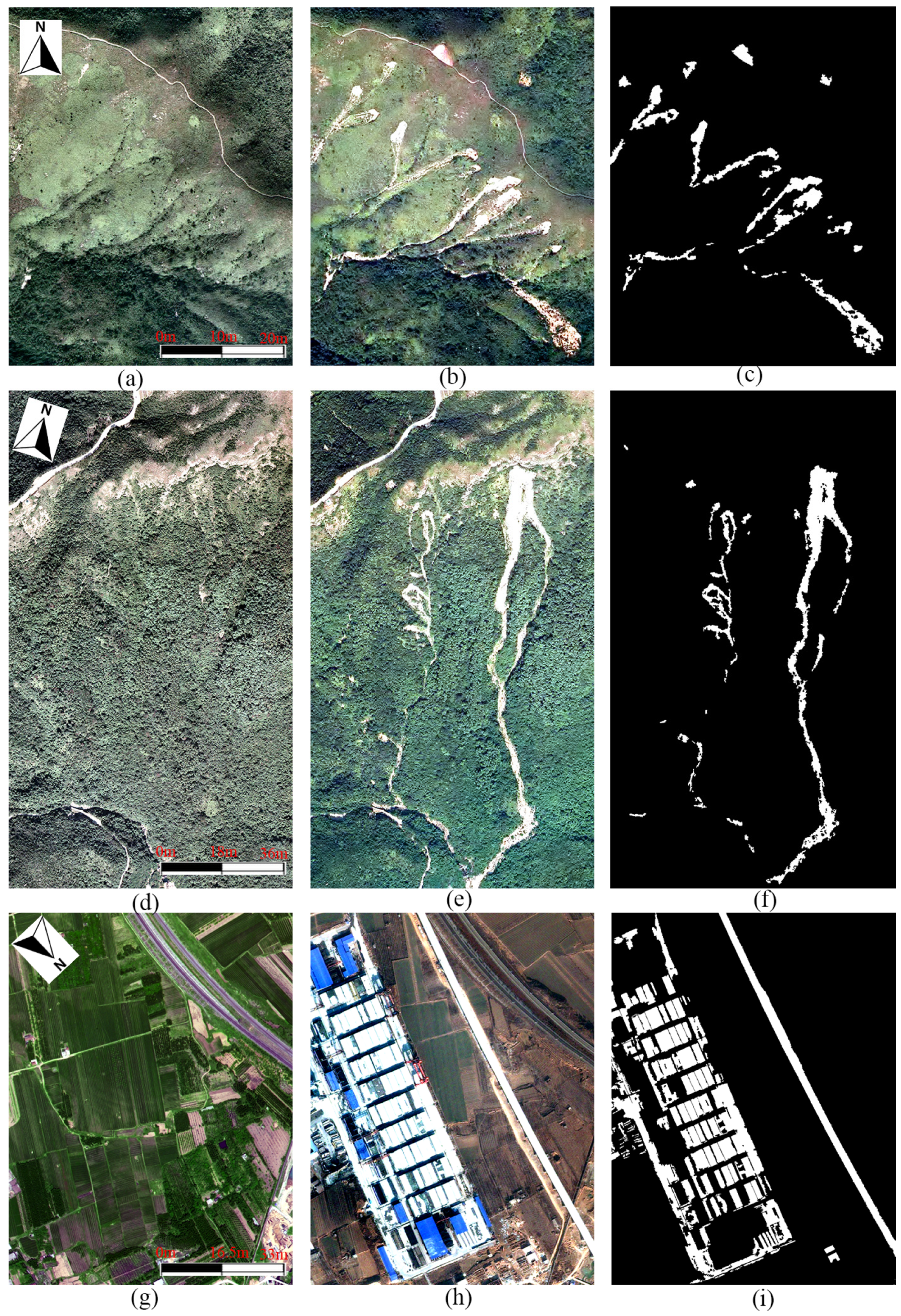
Three pairs of VHR remote sensing images for depicting real land cover change events were employed to assess the effectiveness and performance of our proposed framework. Four state-of-the-art context based LCCD methods and three post-processing LCCD methods were adopted and compared with the proposed framework. Experiments based on the bi-temporal remote sensing images, which covered the real landslide and land use events, were conducted for comparisons. The present study concluded that the proposed LCCD framework based on the integration of spatial–spectral features and multi-scale segmentation voting decision was better suited for the task of change detection than other state-of-the-art techniques.
The rest of this article is divided into four sections. Section 2 describes the proposed methodology. A description of the experimental dataset is given in Section 3. Section 4 presents the details of the experiments and discussion on the results. Conclusions are drawn in Section 5.

2. Methodology

In the present work, a novel framework based on spatial–spectral feature fusion and multi-scale segmentation voting decision for change detection with VHR remote sensing images is proposed. The present work has two contributions: (1) an algorithm based on spatial–spectral feature fusion, Manhattan distance, and Otsu threshold was integrated to obtain the initial BCDMs; and (2) a multi-scale segmentation voting decision method was developed to fuse the initial BCDMs into the final change detection map. Unlike other state-of-the-art techniques that consider only pre- or post- techniques alone, the proposed framework was designed to integrate pre- and post-techniques into a single platform to detect land cover change. As shown in Figure 1, the proposed framework has two major stages, which will be discussed in detail in the following sections.

2.1. Generation of the Initial BCDMs

The aim of the first stage is to generate the initial BCDMs based on spatial–spectral feature fusion. The motivation for fusing different spatial–spectral features lies in that different spatial–spectral features have outstanding different ground targets in an image. One advantage of fusing different spatial–spectral features is that it can enhance the ability to detect a variety of targets. In other words, different spatial–spectral feature extraction methods may have various advantages, and fusing different spatial–spectral features together may provide a potential means of utilizing the advantages of the different spatial–spectral feature extraction methods.
Figure 1a shows the proposed framework of generating the initial BCDMs. First, the spatial feature of the bi-temporal images is extracted using a developed spatial feature extraction method and the spatial and spectral features are stacked with different fusion methods to improve the homogeneity of the target. Second, the Manhattan distance is employed to measure the change magnitude between the corresponding fused feature vector, as presented in Equation (2). Finally, Otsu [56] is applied on the CMI to obtain the binary change detection map.
Three classical spatial feature extraction methods, namely, extended morphological profiles (EMPs) [57], morphological attribute profiles (Aps) [58], and rolling guide filter (RGF) [59], which have been applied successfully for image classification, were introduced to explore the spatial feature of the bi-temporal VHR remote sensing images and verify our viewpoint in the first stage. The spatial and spectral features are denoted as F s p a t 1 = { f s p a 1 , t 1 ,   f s p a 2 , t 1 ,   f s p a 3 , t 1 , , f s p a N , t 1 } and F s p e t 1 = { f s p e 1 , t 1 , f s p e 2 , t 1 , f s p e 3 , t 1 , , f s p e M , t 1 } , respectively.
In this stage, feature fusion is proposed to complement the insufficiency of the spectral information of the VHR remote sensing image. Three feature fusion strategies (layer stacking [35], mean-weight [60] and adaptive weight [61]), which have been applied successfully in road extraction, land cover classification, and image segmentation with VHR remote sensing image, respectively, were proposed. Different strategies have different effects on spatial and spectral features, as shown in Equation (1). For example, the layer stacking method [35] is the most widely used multi-feature fusion approach that concatenates the multiple features into one vector ( W 1 = W 2 = 1.0 ). The mean-weight fusion method [60] separates the effects on F s p a t 1 and F s p e t 1 as 0.5 ( W 1 = W 2 = 0.5 ). In the adaptive weight method [61], the weight of a pixel is determined by the correlation between the center pixel and its surrounding neighbors, and the closer correlation implies a heavier weight, and consequently, more details can be tracked in the literature [61].
F f u s i o n t 1 = { W 1 F s p a t 1 , W 2 F s p e t 1 }
The change magnitude between the bi-temporal images is measured by considering the availability of the Manhattan distance for detecting land cover change [62]. The change magnitude between the corresponding pixel ( P i j t 1 and P i j t 2 ) are calculated using the Manhattan distance [63] as presented in Equation (2). The entire bi-temporal image is processed pixel-by-pixel in this manner and a change magnitude image (CMI) is generated. The spatial–spectral feature used for calculating MD should correspond to the same feature fusion strategy. Therefore, three feature fusion approaches based on one composition of spatial–spectral feature will produce three CMIs.
MD ( P i j t 1 , P i j t 2 ) = F f u s i o n t 1 F f u s i o n t 2
To divide each CMI into a binary change detection map, the binary threshold method, Otsu [56], was employed to divide the CMI into a BCDM. Otsu assumes that the CMI has two classes, changed and unchanged, and calculates the optimum threshold separating the two classes so that their intra-class variance is minimal or equivalent. Otsu has been applied successfully in the prediction of the binary threshold for detecting land cover change (more details can be found in [64,65]).

2.2. Multi-scale Segmentation Voting Decision

In the second stage, the BCDMs are fused into the final change detection map through our proposed multi-scale segmentation voting decision method to further improve the performance of LCCD.
For the second stage, inspired by previous studies [14,49,50], a multi-scale segment voting decision method was developed as a post-processing fusion strategy. Multi-scale segmentation based on the post-event image was acquired using eCognition to ensure that the image was constructed in an object manner (“object” is a group of pixels homogeneous in spectra domain and connected continuously in the spatial domain [66]). Here, the post-event image refers to the image that depicts the occurrence of the detection target such as the landslide or building-up area. Then, the initial BCDMs and multi-scale segmentation were overlapped and the final change detection was generated in an object-by-object manner. In the final change detection map, the label of the pixel within an object was assigned according to the rule of the major voting decision. It is worth noting that the multi-scale segmentation utilized in the proposed approach, called the fractal evolution net approach (FENA) [67], has three parameters (scale, shape, and compactness). In addition, FNEA has been embedded in the eCognition 8.7 software as a “multi-scale segmentation” tool for processing images [68]. The shape and compactness were fixed at 0.8 and 0.9, respectively, because high compactness and homogeneity of segmental objects were expected in our proposed approach.
Combining an image object with MV [49] for fusing and smoothing the initial BCDM has three advantages. (1) The multi-scale segmentation is based on the post-event image and the pixels within an object usually have high-level homogeneity and can be deemed as the same material class. Therefore, some noise pixels can be removed effectively in the final change detection map. (2) The spatial information of the changed or unchanged area such as shape, size, and distribution is obtained from the post-event image through multi-scale segmentation. According to the multi-scale segmentation theory, the shape and size of an object yield to the shape and size of a target or a part of a target. Therefore, smoothing the changed or unchanged area can be done in an adaptive object manner instead of a pixel manner. An adaptive smoothing filter is more rational and practical than using a regular window for detecting land cover change, which is uncertain in terms of shape and size. (3) According to the characteristics of the proposed multi-scale segmentation voting decision strategy, the generation of the final change detection map is acquired by fusing the initial BCDMs. Therefore, the proposed approach has the potential ability to integrate the different advantages of the initial BDCM and improve detection accuracy. A schematic example is presented in Figure 2 to demonstrate the effectiveness of the proposed multi-scale segmentation voting decision.

3. Experiments and Analysis of Results

In this section, three pairs of bi-temporal remote sensing images with very high spatial resolution were used to test the effectiveness of the proposed framework. First, the image data for the three land cover change events were described in detail. Then, the experiments were designed and presented. Finally, the results were compared and the parameter sensitivity of the proposed framework analyzed.

3.1. Dataset Description

The three image datasets used in the experiments are illustrated in Figure 3. These images were acquired through the aerial platform and QuickBird satellite. The images depict landslide change and land use change events. More details on the images are given below and in the caption of Figure 3.
Site A: The bi-temporal images shown in Figure 3a,b were acquired in April 2007 and July 2014, respectively. The bi-temporal image scene depicts the pre- and post-event of a landslide on Lantau Island, Hong Kong, China. The size of this site was 750 × 950 pixels with a spatial resolution of 0.5 m/pixel. The ground reference of the landslide inventory map was interpreted manually as presented in Figure 3c.
Site B: The bi-temporal images of Site B were acquired in the same way as the data for Site A. As shown in Figure 3d,e, the size of the scene was 1252 × 2199 pixels, with a spatial resolution of 0.5 m/pixel. The ground reference of the landslide inventory map of Site B is given in Figure 3f.
Ji’Nan QuickBird data: As shown in Figure 3g–h, the bi-temporal images were acquired by the QuickBird satellite in April 2007 and February 2009, respectively. The size of the image scene was 950 × 1250 pixels with a spatial resolution of 0.61 m/pixel. This area is also covered by different land-use types including crops, naked soil, roads, and railways, and the bi-temporal images are different for each season. These factors pose challenges in detecting land cover changes.
The ground reference of each dataset was interpreted manually. During the progress of interpretation, the bitemporal images were overlayered together. Then, mapping tools such as “Swipe”, “Adjust Transparency”, and the editing toolbars in the ArcMap 10.2, were employed to map the ground reference. In addition, to avoid missing change detection, the changed and unchanged areas were outlined grid-by-grid. Details of the ground reference for each dataset are presented in Table 1.

3.2. Experimental Designation

Three experiments were designed to demonstrate the effectiveness and superiority of the proposed framework in detecting land cover change with VHR remote sensing images.
In the first experiment, bi-temporal images of Site A were used to demonstrate the effectiveness of the proposed framework. The raw spectral features (false color bands) of the bi-temporal images were adopted to detect the landslide area based on the Manhattan distance and Otsu binary threshold. Then, three classic spatial extraction methods (EMPs [57], Aps [58], and RGF [59]) and three multi-features fusion methods (layer stacking [35], mean weight [60], and adaptive weight [61]) were validated in our proposed framework. The parameters of the multi-feature extraction methods are detailed in Table 2.
The superiority of the proposed framework was further investigated in the second experiments. In these experiments, four LCCD methods, namely PCA_Kmeans [40], CVA_FCM [41], Semi_FCM [42], and LSELUC [43], which also consider contextual information to improve the detection accuracy and have been applied successfully in practice, were used. The landslide Site B aerial and Ji’Nan QuickBird satellite images were employed for comparisons in each experiment. The optimized parameter settings of these approaches and datasets are given in Table 3.
Three post-processing LCCD methods (MV [49], GPCF [50], and OBEM [51]) were employed and compared with the proposed framework based on the Site B and Ji’Nan datasets to further demonstrate the advantages of the proposed framework. The optimal parameters of the post-processing LCCD methods are presented as follows.
First, as the proposed approach concentrated on detecting the land cover change and guarantee the fairness of comparison, the parameters of the spatial feature extraction methods were fixed for each dataset, as shown in Table 2. Moreover, the generation of CMI and BCDM for all post-processing approaches was also based on the MD distance and Otsu binary threshold method. Second, in addition to the parameter settings for spatial feature extraction, the parameters for each post-processing approach were optimized using the trial-and-error approach. The optimized parameters of each post-approach and dataset are detailed in Table 4.

4. Results and Analysis

Various measuring indices were considered in the quantitative assessment of the proposed framework: the ratio of false alarms (FA), the ratio of missed alarms (MA), the ratio of total errors (TE), overall accuracy (OA), and Kappa coefficient (Ka). All performance measuring indices were considered for a comparative analysis of the experiments.
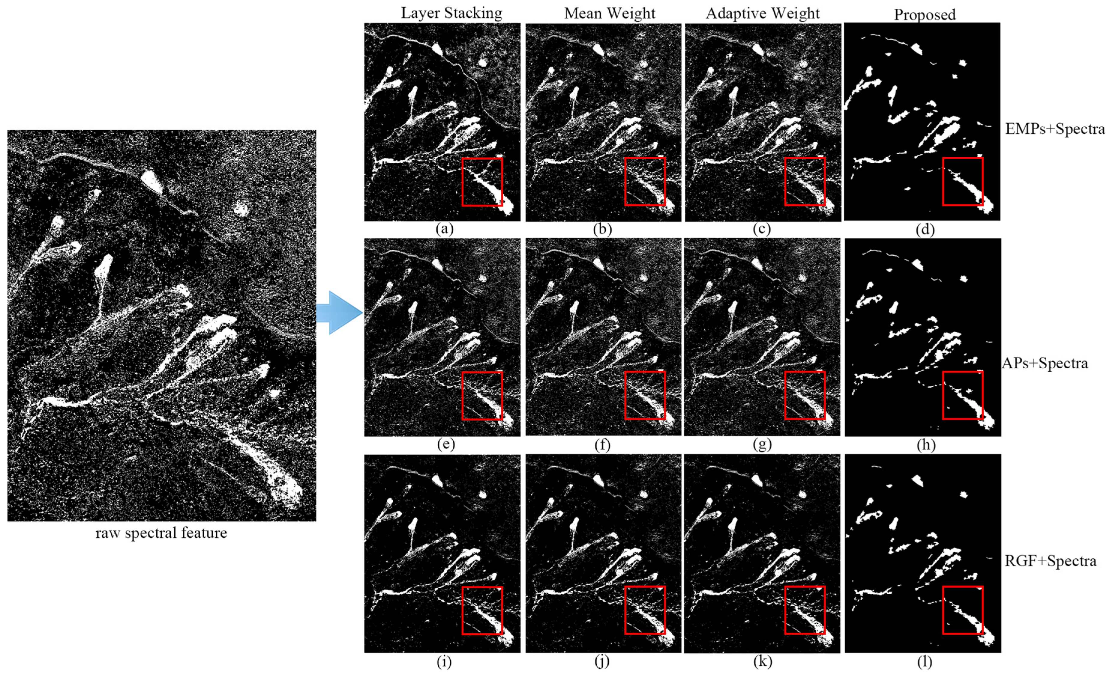
As mentioned in the above sections, evaluation of the effectiveness of the proposed method, raw spectral feature, three spatial-spectral feature fusion approaches (layer stacking [35], mean-weight [60], and adaptive weight [61]), and the proposed framework was applied on the Site A VHR bi-temporal images for comparison. Table 5 shows that compared with methods that use the raw spectral feature alone, the spatial feature coupled with the spectral feature could clearly improve the cover detection accuracies. For instance, the improvement of FA was about 5.98% in terms of the layer stacking fusion approach [35] and the EMPs spatial feature extraction approach [57]. Furthermore, the proposed approach achieved the best detection accuracies when compared with the spatial–spectral feature fusion-based approach and that of using the raw spectral feature alone. Figure 4 demonstrates that the proposed framework clearly smoothened the salt-and-pepper noise in the results using the raw spectral feature alone and each spatial–spectral feature fusion-based approach.
The proposed approach was compared with state-of-the-art LCCD methods including PCA_Kmean [40], CVA_FCM [41], Semi_FCM [42], and LSELUC [43] to further outline the advantages of the proposed framework. For experimentation, two pairs of VHR remote sensing images were considered for comparison. 
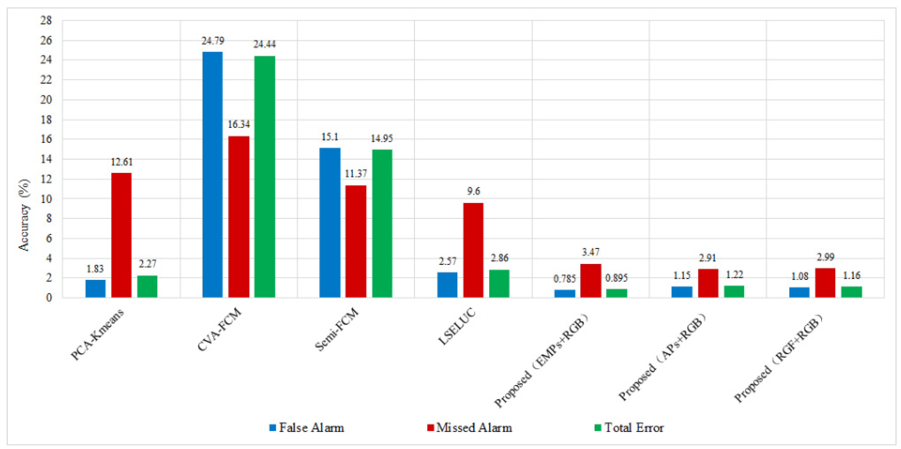
Table 6 shows the results of the comparison of the Site B landslide aerial remote sensing images with state-of-the-art methods. The advantages of the proposed approach can be found in three ways: (1) The results showed that among the state-of-the art methods, the relatively new LSELUC approach achieved better accuracies because reliable local spatial information was considered through local uncertainties in the developed LSELUC approach. However, the detection accuracies of the proposed framework achieved the best accuracies in terms of FA, MA, TE, OA, and Ka; (2) Different spatial–spatial feature fusion methods that may have different effects on the performance of the proposed framework were adopted in the proposed framework; however, the best accuracy could be achieved by the proposed framework regardless of which spatial–spectra feature fusion method was adopted; and (3) For the Site B aerial images, EMPs [57] coupled with spectral feature in the proposed approach acquired the best accuracies.
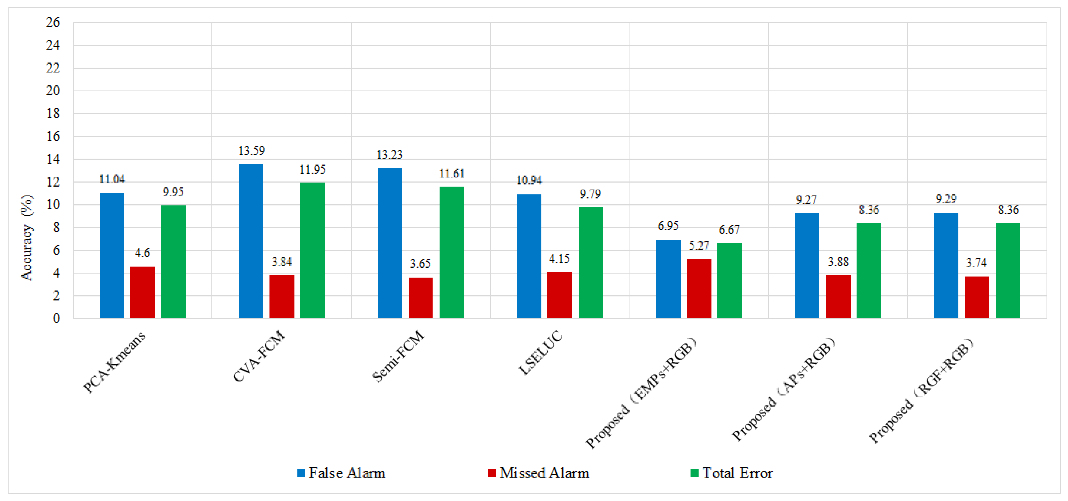
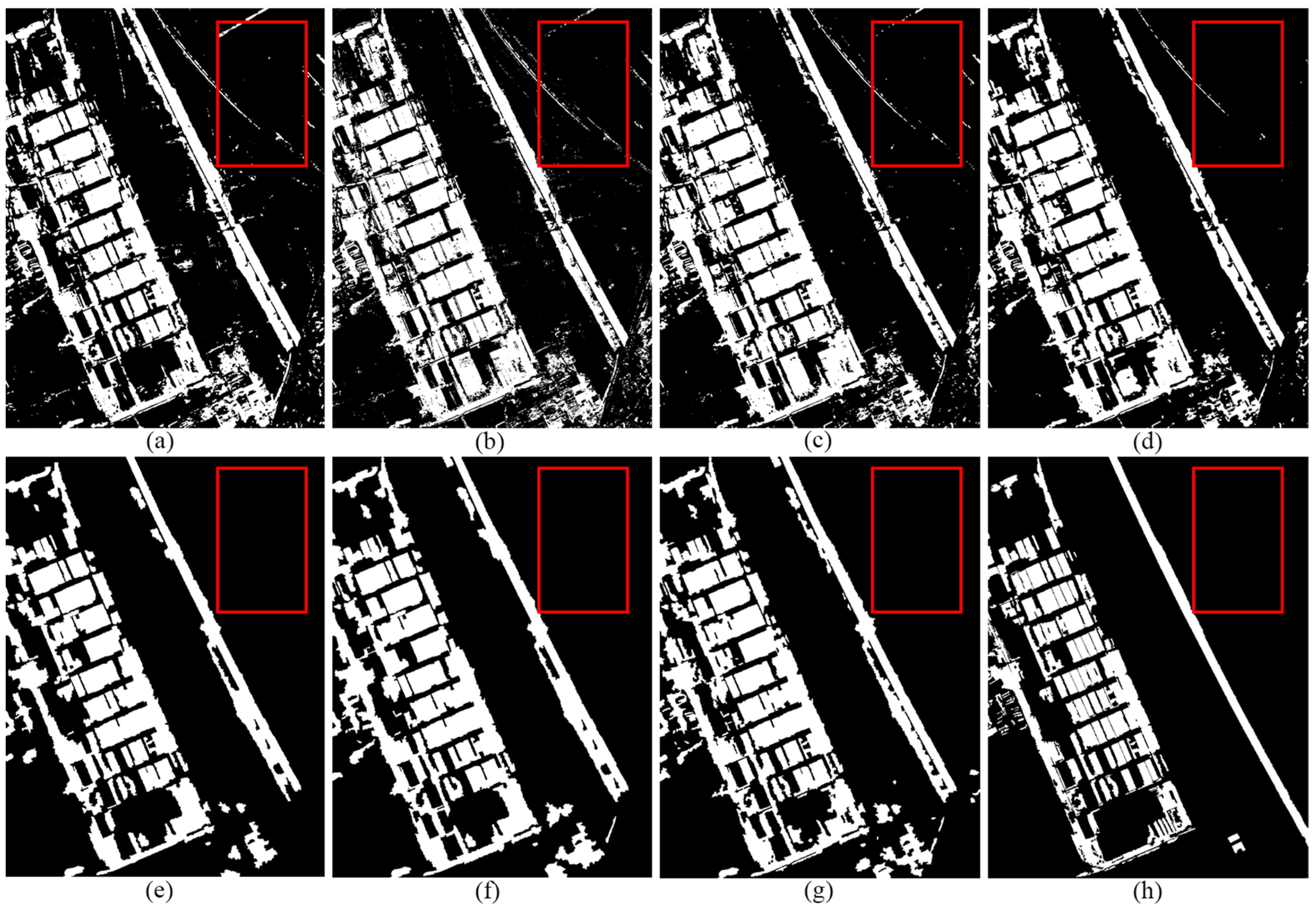
Comparisons among the approaches were performed as shown in the bar charts of Figure 5. The figure clearly presents the advantages of the proposed approach. The visual performance of the comparisons further verified the conclusion of comparisons of the Site B landslide aerial images as shown in Figure 6. The comparisons on the Ji’Nan QuickBird satellite images for detecting land cover and land use change were conducted and similar conclusions were reached. The details can be found in Table 7 and Figure 7 and Figure 8. From the quantitative comparisons and visual performance, it can be seen that the proposed approach achieved the best accuracies in terms of FA, MA, and TA, regardless of the utilized spatial feature extraction approach that was employed.
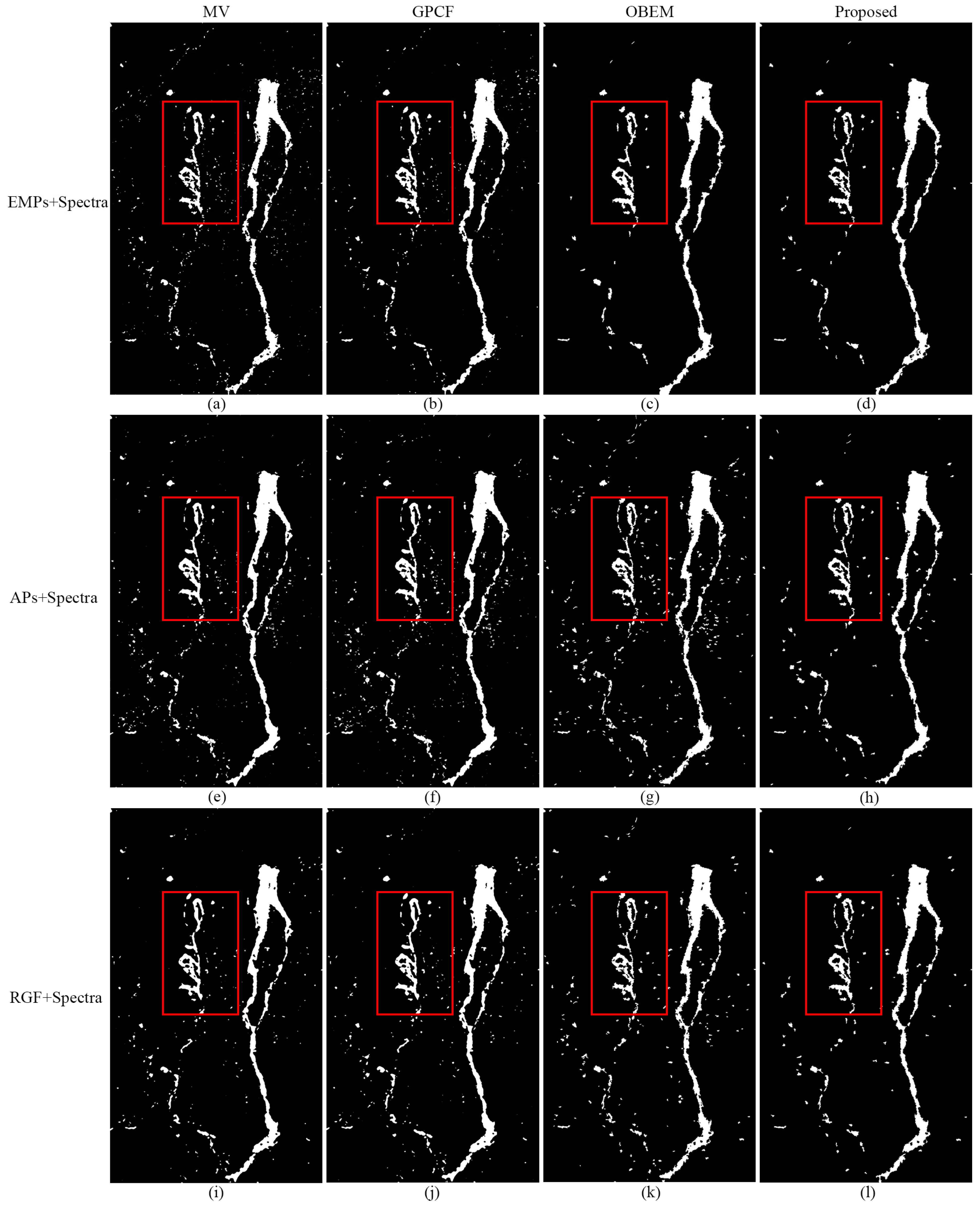
The proposed approach was compared with MV [49], GPCF [50], and OBEM [51] to further investigate the advantages of the proposed approach as designed in the third experiment. The comparative results for the Site B landslide aerial images are shown in Table 8. From these comparisons, the proposed approach appears to have achieved a competitive detection accuracy when compared with that of MV [49], GPCF [50], and OBEM [51]. In addition, while visual performance was observed as shown in Figure 9, the proposed approach (the fourth column in Figure 9) presented less noise than the others. This finding was further verified in the quantitative comparison in Table 9. A similar conclusion can be reached from the comparisons conducted on the Ji’Nan QB satellite remote sensing images shown in Table 9 and Figure 10.
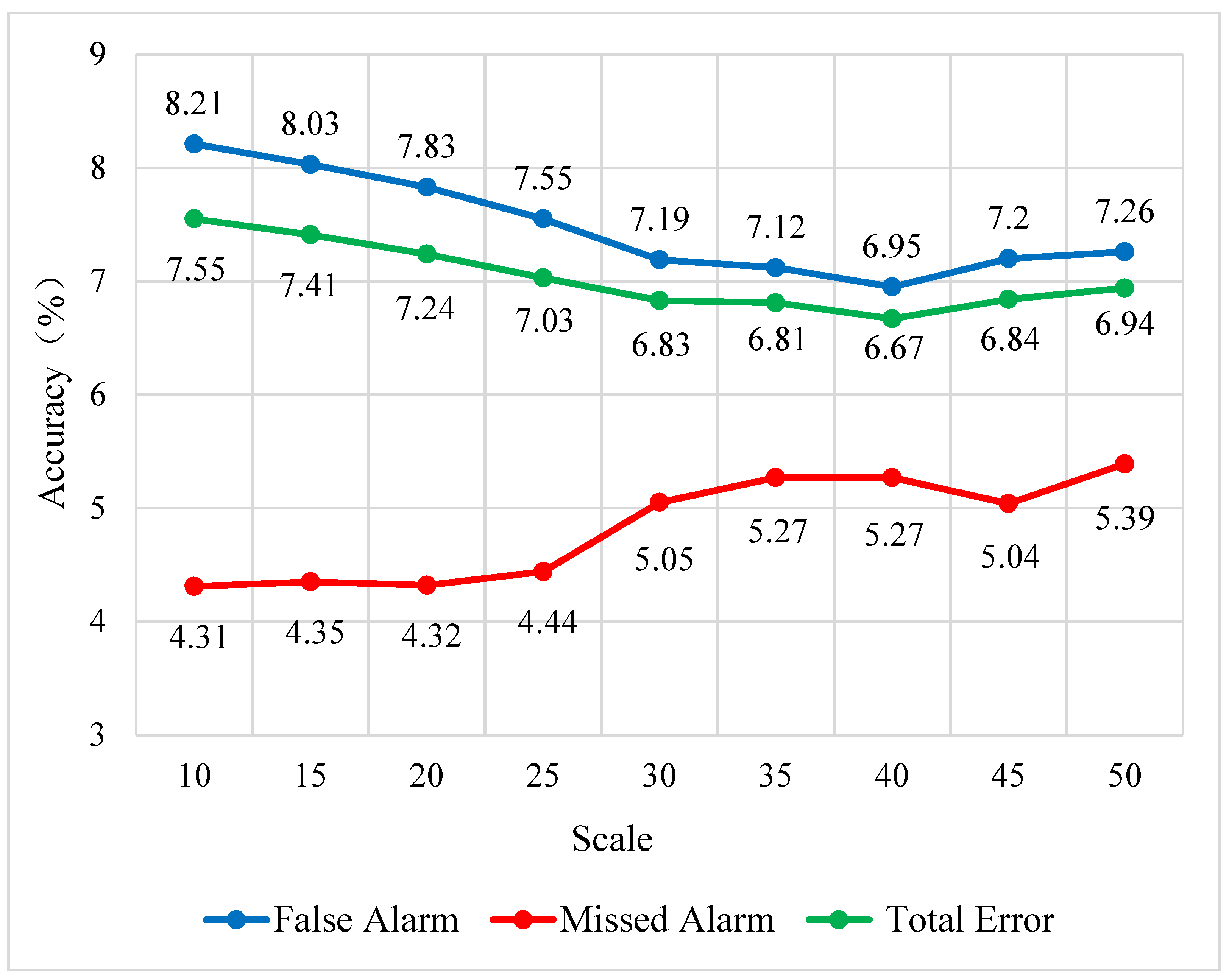
The sensitivity of the detection accuracy and the parameters of the proposed approach are discussed in this section with the aim of extending the potential application of the proposed approach. We only observed the relationship between scale and detection accuracies. Parameter scale indicates the size of the segmental object and a larger scale will generate larger segments and the ground details of a target may be smoothened. In contrast, a smaller scale will yield a smaller segment and more ground detail will be preserved. However, more noise will be introduced to the detection results. Therefore, an appropriate scale should be adjusted according to the given images.
Figure 11 shows that MA, TE, and FA decreased as the scale increased. Furthermore, MA and TE decreased gradually when the scale ranged from 10 to 30. However, when the value of the scale was larger than 30, MA and TE remained at a horizontal level. These results can be attributed to the size of the segments being large enough to obtain optimum accuracy because the scale has less effect on the size of the segments as the other parameters (compactness and shape) are fixed. In addition to MA and TE, FA also decreased as the scale increased and then fluctuated in the range of 2.99 to 3.91. This fluctuation may be caused by the uncertain distribution of spatial heterogeneity.
The relationship between the segmental scale and the detection accuracy in the Ji’Nan QB satellite images was also investigated. Figure 12 shows that for the Ji’Nan dataset, FA and TE decreased as the scale increased, and MA first increased then decreased. These findings are helpful in determining the parameters of the proposed approach.

5. Conclusions

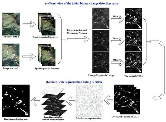
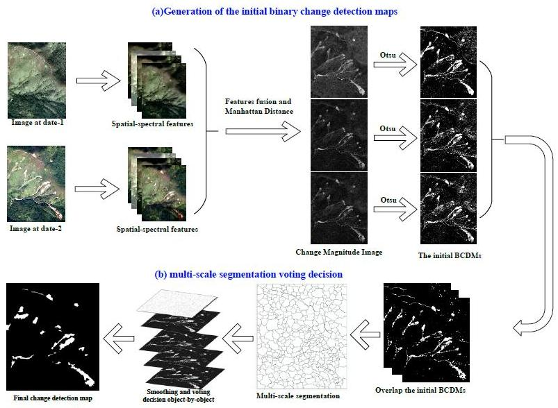
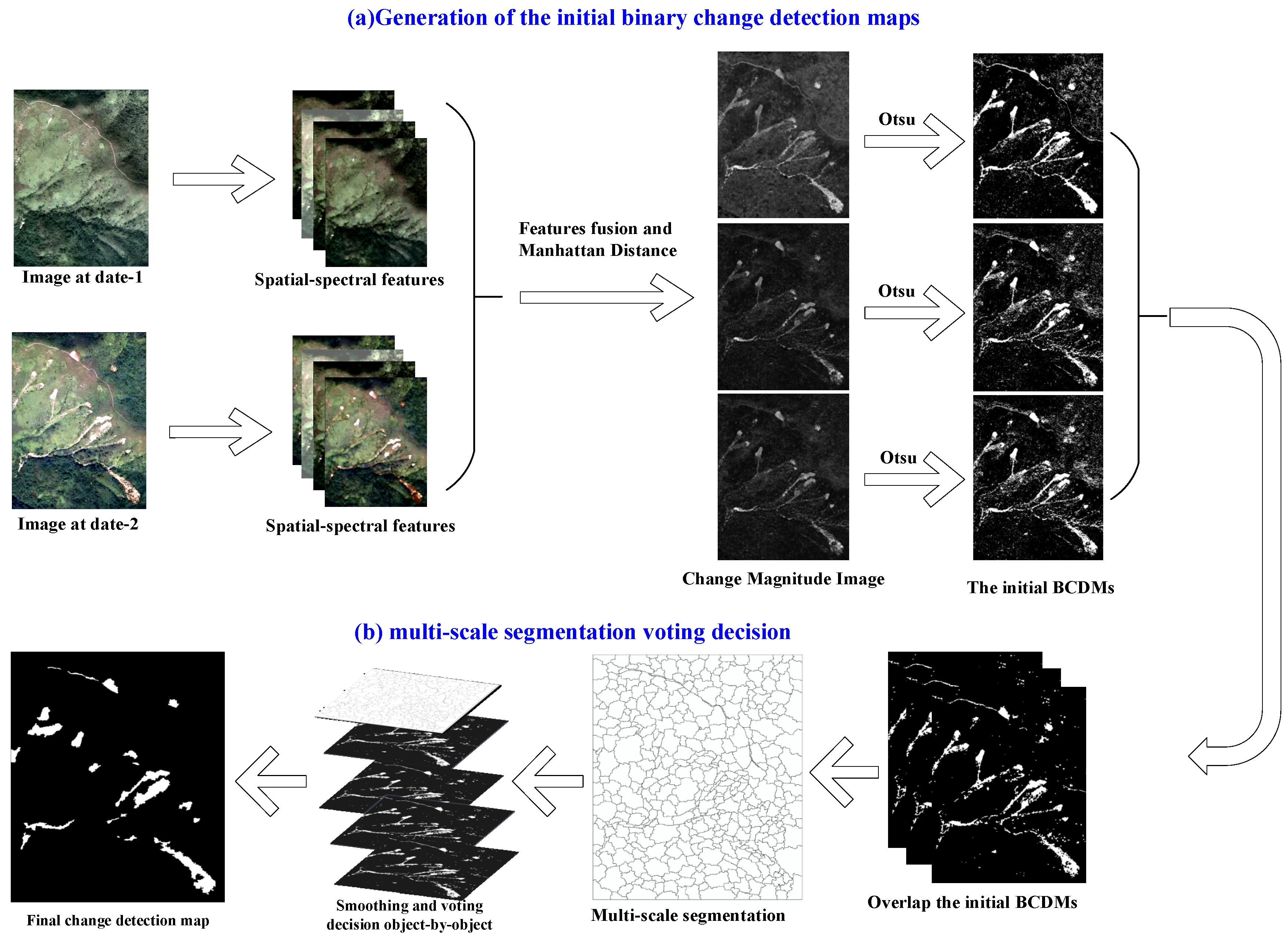
In the present work, a novel framework for detecting land cover change using spatial–spectral feature fusion and multi-scale segmentation voting decision strategies was proposed. Instead of using a single feature to obtain the binary change detection map directly, spatial features were extracted and coupled with the raw spectral feature through different fusion strategies. Different spatial–spectral features were provided with different initial BCDMs. Finally, a multi-scale segmentation voting decision strategy was proposed to fuse the initial BCDMs into the final change detection map. The main contribution of the proposed approach was that it provides a comprehensive framework for more accurate land cover change detection using bitemporal VHR remote sensing images. Multi-spatial features and different feature fusion strategies were introduced to generate the initial BCDMs. In addition, multi-scale segmentation voting decision was first promoted to fuse the initial BCDMs into the final change detection map. The advantages of multi-scale segmentation voting decision have two aspects: (1) the different performance of the initial BCMDs, which are obtained from different spatial–spectral features, can be utilized together to avoid the bias detection; and (2) majority voting with the constraint of a multi-scale object can consider the uncertainty of the ground target such as the shape and size of a target, which is helpful in improving the voting accuracy.
Experiments were carried out on three pairs of datasets to confirm the effectiveness of the proposed approach. The results of the experiments showed that the proposed approach achieved better performance than using the raw spectral feature alone and other state-of-the-art LCCD techniques. However, one limitation of the proposed framework is that it requires many parameters in practical application, and the optimized parameter setting for a specific dataset is time-consuming. In the future, an extensive investigation of the proposed approach will be conducted on additional types of images and land cover change events such as unmanned aerial vehicle images and forest disasters. Theoretically, further investigations on a method with various sourcing image and land cover change events will improve the robustness of the method. A comprehensive investigation will also broaden the applicability of the proposed approach.

Author Contributions

Conceptualization, Z.Z. and J.C.; methodology, Z.L.; software, Z.L.; validation, Z.Z.; formal analysis, J.A.B.; investigation, Z.Z.; resources, Z.Z.; data curation, Z.Z.; writing—original draft preparation, Z.Z.; writing—review and editing, J.A.B.; visualization, Z.L.; supervision, J.C.; project administration, J.C.; funding acquisition, J.C.

Funding

This research was funded by National Natural Science Foundation of China (Grant Number 41571346 and 61701396), the Natural Science Foundation of Shaan Xi Province (2018JQ4009), and the Open Fund for Key laboratory of Degraded and Unused Land Consolidation Engineering, the Ministry of Natural Resource (Grant number SXDJ2017-10 and 2016KCT-23).

Acknowledgments

The authors would like to express their gratitude to the Editor-in-Chief, the associate editors, and the reviewers for their insightful comments and suggestions. In addition, we want to thanks the Lands Department of the Government of the Hong Kong Special Administrative Region of the People’s Republic of China provides the aerial photos of the landslides in Lantau Island area.

Conflicts of Interest

The authors declare no conflicts of interest.

References

  1. Singh, A. Review article digital change detection techniques using remotely-sensed data. Int. J. Remote Sens. 1989, 10, 989–1003. [Google Scholar] [CrossRef]
  2. Coppin, P.; Jonckheere, I.; Nackaerts, K.; Muys, B.; Lambin, E. Review articledigital change detection methods in ecosystem monitoring: A review. Int. J. Remote Sens. 2004, 25, 1565–1596. [Google Scholar] [CrossRef]
  3. Zhu, Z. Change detection using landsat time series: A review of frequencies, preprocessing, algorithms, and applications. ISPRS J. Photogramm. Remote Sens. 2017, 130, 370–384. [Google Scholar] [CrossRef]
  4. Mahabir, R.; Croitoru, A.; Crooks, A.; Agouris, P.; Stefanidis, A. A critical review of high and very high-resolution remote sensing approaches for detecting and mapping slums: Trends, challenges and emerging opportunities. Urban Sci. 2018, 2, 8. [Google Scholar] [CrossRef]
  5. Hansen, M.C.; Loveland, T.R. A review of large area monitoring of land cover change using landsat data. Remote Sens. Environ. 2012, 122, 66–74. [Google Scholar] [CrossRef]
  6. Tian, D.; Gong, M. A novel edge-weight based fuzzy clustering method for change detection in sar images. Inf. Sci. 2018, 467, 415–430. [Google Scholar] [CrossRef]
  7. Song, X.-P.; Hansen, M.C.; Stehman, S.V.; Potapov, P.V.; Tyukavina, A.; Vermote, E.F.; Townshend, J.R. Global land change from 1982 to 2016. Nature 2018, 560, 639. [Google Scholar] [CrossRef]
  8. Chen, J.; Chen, J.; Liao, A.; Cao, X.; Chen, L.; Chen, X.; He, C.; Han, G.; Peng, S.; Lu, M. Global land cover mapping at 30 m resolution: A pok-based operational approach. ISPRS J. Photogramm. Remote Sens. 2015, 103, 7–27. [Google Scholar] [CrossRef]
  9. Zanotta, D.C.; Haertel, V. Gradual land cover change detection based on multitemporal fraction images. Pattern Recognit. 2012, 45, 2927–2937. [Google Scholar] [CrossRef]
  10. Erb, K.-H.; Kastner, T.; Plutzar, C.; Bais, A.L.S.; Carvalhais, N.; Fetzel, T.; Gingrich, S.; Haberl, H.; Lauk, C.; Niedertscheider, M. Unexpectedly large impact of forest management and grazing on global vegetation biomass. Nature 2018, 553, 73. [Google Scholar] [CrossRef]
  11. Forkan, A.R.M.; Khalil, I.; Tari, Z.; Foufou, S.; Bouras, A. A context-aware approach for long-term behavioural change detection and abnormality prediction in ambient assisted living. Pattern Recognit. 2015, 48, 628–641. [Google Scholar] [CrossRef]
  12. Li, Z.; Shi, W.; Lu, P.; Yan, L.; Wang, Q.; Miao, Z. Landslide mapping from aerial photographs using change detection-based markov random field. Remote Sens. Environ. 2016, 187, 76–90. [Google Scholar] [CrossRef]
  13. Li, Z.; Shi, W.; Myint, S.W.; Lu, P.; Wang, Q. Semi-automated landslide inventory mapping from bitemporal aerial photographs using change detection and level set method. Remote Sens. Environ. 2016, 175, 215–230. [Google Scholar] [CrossRef]
  14. Lv, Z.Y.; Shi, W.; Zhang, X.; Benediktsson, J.A. Landslide inventory mapping from bitemporal high-resolution remote sensing images using change detection and multiscale segmentation. IEEE J. Sel. Top. Appl. Earth Obs. Remote Sens. 2018, 11, 1520–1532. [Google Scholar] [CrossRef]
  15. Hansen, M.C.; Potapov, P.V.; Moore, R.; Hancher, M.; Turubanova, S.; Tyukavina, A.; Thau, D.; Stehman, S.; Goetz, S.; Loveland, T.R. High-resolution global maps of 21st-century forest cover change. Science 2013, 342, 850–853. [Google Scholar] [CrossRef] [PubMed]
  16. Bruzzone, L.; Bovolo, F. A novel framework for the design of change-detection systems for very-high-resolution remote sensing images. Proc. IEEE 2013, 101, 609–630. [Google Scholar] [CrossRef]
  17. Moser, G.; Serpico, S.B.; Benediktsson, J.A. Land-cover mapping by markov modeling of spatial–contextual information in very-high-resolution remote sensing images. Proc. IEEE 2013, 101, 631–651. [Google Scholar] [CrossRef]
  18. Zhang, W.; Tan, G.; Zheng, S.; Sun, C.; Kong, X.; Liu, Z. Land cover change detection in urban lake areas using multi-temporary very high spatial resolution aerial images. Water 2018, 10, 1. [Google Scholar] [CrossRef]
  19. Roy, M.; Ghosh, S.; Ghosh, A. A novel approach for change detection of remotely sensed images using semi-supervised multiple classifier system. Inf. Sci. 2014, 269, 35–47. [Google Scholar] [CrossRef]
  20. Bruzzone, L.; Prieto, D.F. Automatic analysis of the difference image for unsupervised change detection. IEEE Trans. Geosci. Remote Sens. 2000, 38, 1171–1182. [Google Scholar] [CrossRef] [Green Version]
  21. Radke, R.J.; Andra, S.; Al-Kofahi, O.; Roysam, B. Image change detection algorithms: A systematic survey. IEEE Trans. Image Process. 2005, 14, 294–307. [Google Scholar] [CrossRef] [PubMed]
  22. Homer, C.; Dewitz, J.; Yang, L.; Jin, S.; Danielson, P.; Xian, G.; Coulston, J.; Herold, N.; Wickham, J.; Megown, K. Completion of the 2011 national land cover database for the conterminous United States–representing a decade of land cover change information. Photogramm. Eng. Remote Sens. 2015, 81, 345–354. [Google Scholar]
  23. Otukei, J.R.; Blaschke, T. Land cover change assessment using decision trees, support vector machines and maximum likelihood classification algorithms. Int. J. Appl. Earth Obs. Geoinf. 2010, 12, S27–S31. [Google Scholar] [CrossRef]
  24. Ye, S.; Chen, D.; Yu, J. A targeted change-detection procedure by combining change vector analysis and post-classification approach. ISPRS J. Photogramm. Remote Sens. 2016, 114, 115–124. [Google Scholar] [CrossRef]
  25. Lu, D.; Mausel, P.; Brondizio, E.; Moran, E. Change detection techniques. Int. J. Remote Sens. 2004, 25, 2365–2401. [Google Scholar] [CrossRef]
  26. Lv, Z.; Liu, T.; Benediktsson, J.A.; Du, H. A novel land cover change detection method based on k-means clustering and adaptive majority voting using bitemporal remote sensing images. IEEE Access 2019, 7, 34425–34437. [Google Scholar] [CrossRef]
  27. Chen, X.; Chen, J.; Shi, Y.; Yamaguchi, Y. An automated approach for updating land cover maps based on integrated change detection and classification methods. ISPRS J. Photogramm. Remote Sens. 2012, 71, 86–95. [Google Scholar] [CrossRef]
  28. Aguirre-Gutiérrez, J.; Seijmonsbergen, A.C.; Duivenvoorden, J.F. Optimizing land cover classification accuracy for change detection, a combined pixel-based and object-based approach in a mountainous area in Mexico. Appl. Geogr. 2012, 34, 29–37. [Google Scholar] [CrossRef] [Green Version]
  29. Shi, C.; Pun, C.-M. Adaptive multi-scale deep neural networks with perceptual loss for panchromatic and multispectral images classification. Inf. Sci. 2019, 490, 1–17. [Google Scholar] [CrossRef]
  30. Yu, W.; Zhou, W.; Qian, Y.; Yan, J. A new approach for land cover classification and change analysis: Integrating backdating and an object-based method. Remote Sens. Environ. 2016, 177, 37–47. [Google Scholar] [CrossRef]
  31. Tarantino, C.; Adamo, M.; Lucas, R.; Blonda, P. Detection of changes in semi-natural grasslands by cross correlation analysis with worldview-2 images and new landsat 8 data. Remote Sens. Environ. 2016, 175, 65–72. [Google Scholar] [CrossRef] [PubMed]
  32. Tewkesbury, A.P.; Comber, A.J.; Tate, N.J.; Lamb, A.; Fisher, P.F. A critical synthesis of remotely sensed optical image change detection techniques. Remote Sens. Environ. 2015, 160, 1–14. [Google Scholar] [CrossRef] [Green Version]
  33. Ghamisi, P.; Dalla Mura, M.; Benediktsson, J.A. A survey on spectral–spatial classification techniques based on attribute profiles. IEEE Trans. Geosci. Remote Sens. 2015, 53, 2335–2353. [Google Scholar] [CrossRef]
  34. Fauvel, M.; Tarabalka, Y.; Benediktsson, J.A.; Chanussot, J.; Tilton, J.C. Advances in spectral-spatial classification of hyperspectral images. Proc. IEEE 2013, 101, 652–675. [Google Scholar] [CrossRef]
  35. Huang, X.; Zhang, L. An svm ensemble approach combining spectral, structural, and semantic features for the classification of high-resolution remotely sensed imagery. IEEE Trans. Geosci. Remote Sens. 2013, 51, 257–272. [Google Scholar] [CrossRef]
  36. Immitzer, M.; Atzberger, C.; Koukal, T. Tree species classification with random forest using very high spatial resolution 8-band worldview-2 satellite data. Remote Sens. 2012, 4, 2661–2693. [Google Scholar] [CrossRef]
  37. Liu, R.; Li, W.; Liu, X.; Lu, X.; Li, T.; Guo, Q. An ensemble of classifiers based on positive and unlabeled data in one–class remote sensing classification. IEEE J. Sel. Top. Appl. Earth Obs. Remote Sens. 2018, 11, 572–584. [Google Scholar] [CrossRef]
  38. Sinha, P.; Kumar, L. Binary images in seasonal land-cover change identification: A comparative study in parts of New South Wales, Australia. Int. J. Remote Sens. 2013, 34, 2162–2186. [Google Scholar] [CrossRef]
  39. Zhang, P.; Lv, Z.; Shi, W. Local spectrum-trend similarity approach for detecting land-cover change by using spot-5 satellite images. IEEE Geosci. Remote Sens. Lett. 2014, 11, 738–742. [Google Scholar] [CrossRef]
  40. Celik, T. Unsupervised change detection in satellite images using principal component analysis and $ k $-means clustering. IEEE Geosci. Remote Sens. Lett. 2009, 6, 772–776. [Google Scholar] [CrossRef]
  41. Liu, S.; Bruzzone, L.; Bovolo, F.; Zanetti, M.; Du, P. Sequential spectral change vector analysis for iteratively discovering and detecting multiple changes in hyperspectral images. IEEE Trans. Geosci. Remote Sens. 2015, 53, 4363–4378. [Google Scholar] [CrossRef]
  42. Shao, P.; Shi, W.; He, P.; Hao, M.; Zhang, X. Novel approach to unsupervised change detection based on a robust semi-supervised fcm clustering algorithm. Remote Sens. 2016, 8, 264. [Google Scholar] [CrossRef]
  43. Zhang, X.; Shi, W.; Liang, P.; Hao, M. Level set evolution with local uncertainty constraints for unsupervised change detection. Remote Sens. Lett. 2017, 8, 811–820. [Google Scholar] [CrossRef]
  44. Dey, V.; Zhang, Y.; Zhong, M. A review on image segmentation techniques with remote sensing perspective. ISPRS 2010, 38, 31–42. [Google Scholar]
  45. Li, Z.; Shi, W.; Zhang, H.; Hao, M. Change detection based on gabor wavelet features for very high resolution remote sensing images. IEEE Geosci. Remote Sens. Lett. 2017, 14, 783–787. [Google Scholar] [CrossRef]
  46. Zhou, L.; Cao, G.; Li, Y.; Shang, Y. Change detection based on conditional random field with region connection constraints in high-resolution remote sensing images. IEEE J. Sel. Top. Appl. Earth Obs. Remote Sens. 2016, 9, 3478–3488. [Google Scholar] [CrossRef]
  47. Blaschke, T. Towards a framework for change detection based on image objects. Gött. Geogr. Abh. 2005, 113, 1–9. [Google Scholar]
  48. Huang, X.; Zhang, L.; Gong, W. Information fusion of aerial images and lidar data in urban areas: Vector-stacking, re-classification and post-processing approaches. Int. J. Remote Sens. 2011, 32, 69–84. [Google Scholar] [CrossRef]
  49. Huang, X.; Lu, Q.; Zhang, L.; Plaza, A. New postprocessing methods for remote sensing image classification: A systematic study. IEEE Trans. Geosci. Remote Sens. 2014, 52, 7140–7159. [Google Scholar] [CrossRef]
  50. Lv, Z.; Zhang, X.; Benediktsson, J.A. Developing a general post-classification framework for land-cover mapping improvement using high-spatial-resolution remote sensing imagery. Remote Sens. Lett. 2017, 8, 607–616. [Google Scholar] [CrossRef]
  51. Lv, Z.; Liu, T.; Wan, Y.; Benediktsson, J.A.; Zhang, X. Post-processing approach for refining raw land cover change detection of very high-resolution remote sensing images. Remote Sens. 2018, 10, 472. [Google Scholar] [CrossRef]
  52. Hecheltjen, A.; Thonfeld, F.; Menz, G. Recent advances in remote sensing change detection–A review. In Land Use and Land Cover Mapping in Europe; Springer: Berlin, Germany, 2014; pp. 145–178. [Google Scholar]
  53. Huang, X.; Zhang, L.; Li, P. A multiscale feature fusion approach for classification of very high resolution satellite imagery based on wavelet transform. Int. J. Remote Sens. 2008, 29, 5923–5941. [Google Scholar] [CrossRef]
  54. Chaib, S.; Liu, H.; Gu, Y.; Yao, H. Deep feature fusion for vhr remote sensing scene classification. IEEE Trans. Geosci. Remote Sens. 2017, 55, 4775–4784. [Google Scholar] [CrossRef]
  55. Zhao, J.; Zhong, Y.; Shu, H.; Zhang, L. High-resolution image classification integrating spectral-spatial-location cues by conditional random fields. IEEE Trans. Image Process. 2016, 25, 4033–4045. [Google Scholar] [CrossRef] [PubMed]
  56. Otsu, N. A threshold selection method from gray-level histograms. IEEE Trans. Syst. Man Cybern. 1979, 9, 62–66. [Google Scholar] [CrossRef]
  57. Benediktsson, J.A.; Palmason, J.A.; Sveinsson, J.R. Classification of hyperspectral data from urban areas based on extended morphological profiles. IEEE Trans. Geosci. Remote Sens. 2005, 43, 480–491. [Google Scholar] [CrossRef]
  58. Dalla Mura, M.; Benediktsson, J.A.; Waske, B.; Bruzzone, L. Morphological attribute profiles for the analysis of very high resolution images. IEEE Trans. Geosci. Remote Sens. 2010, 48, 3747–3762. [Google Scholar] [CrossRef]
  59. Huang, X.; Lu, Q.; Zhang, L. A multi-index learning approach for classification of high-resolution remotely sensed images over urban areas. ISPRS J. Photogramm. Remote Sens. 2014, 90, 36–48. [Google Scholar] [CrossRef]
  60. Li, F.; Wang, J.; Lan, R.; Liu, Z.; Luo, X. Hyperspectral image classification using multi-feature fusion. Opt. Laser Technol. 2019, 110, 176–183. [Google Scholar] [CrossRef]
  61. Chen, Q.; Chen, Y. Multi-feature object-based change detection using self-adaptive weight change vector analysis. Remote Sens. 2016, 8, 549. [Google Scholar] [CrossRef]
  62. Xue, Z.; Du, P.; Feng, L. Phenology-driven land cover classification and trend analysis based on long-term remote sensing image series. IEEE J. Sel. Top. Appl. Earth Obs. Remote Sens. 2014, 7, 1142–1156. [Google Scholar] [CrossRef]
  63. Perlibakas, V. Distance measures for pca-based face recognition. Pattern Recognit. Lett. 2004, 25, 711–724. [Google Scholar] [CrossRef]
  64. Lv, Z.; Shi, W.; Zhou, X.; Benediktsson, J. Semi-automatic system for land cover change detection using bi-temporal remote sensing images. Remote Sens. 2017, 9, 1112. [Google Scholar] [CrossRef]
  65. Sezgin, M.; Sankur, B. Survey over image thresholding techniques and quantitative performance evaluation. J. Electron. Imag. 2004, 13, 146–166. [Google Scholar]
  66. Blaschke, T.; Hay, G.J.; Kelly, M.; Lang, S.; Hofmann, P.; Addink, E.; Feitosa, R.Q.; Van der Meer, F.; Van der Werff, H.; Van Coillie, F. Geographic object-based image analysis–towards a new paradigm. ISPRS J. Photogramm. Remote Sens. 2014, 87, 180–191. [Google Scholar] [CrossRef] [PubMed]
  67. Taubenböck, H.; Esch, T.; Wurm, M.; Roth, A.; Dech, S. Object-based feature extraction using high spatial resolution satellite data of urban areas. J. Spat. Sci. 2010, 55, 117–132. [Google Scholar] [CrossRef]
  68. Yang, Y.; Li, H.; Han, Y.; Gu, H. High resolution remote sensing image segmentation based on graph theory and fractal net evolution approach. Int. Arch. Photogramm. Remote Sens. Spat. Inf. Sci 2015, 40, 197–201. [Google Scholar] [CrossRef]
Figure 1. Flowchart of the proposed framework based on the multi-feature fusion and multi-scale segmentation voting decision.
Remotesensing 11 01903 g001
Figure 2. Example of the proposed multi-scale segmentation voting decision.
Remotesensing 11 01903 g002
Figure 3. False color bi-temporal images for land cover change detection: (a) Pre-landslide image of Hong Kong, Site A; (b) Post-landslide image of Hong Kong, Site A; (c) Ground reference for the landslide in Hong Kong, Site A; (d) Pre-landslide image of Hong Kong, Site B; (e) Post-landslide image of Hong Kong, Site B; (f) Ground reference for the landslide in Hong Kong, Site B; (g) Pre-event image of Ji’Nan QuickBird data; (h) Post-event image of Ji’Nan QuickBird data; (i) Ground reference for the Ji’Nan QuickBird.
Remotesensing 11 01903 g003
Figure 4. The comparison between the proposed framework and that using the raw spectral feature alone indicates that the results achieved by the proposed approach performed with less salt-and-pepper noise, as highlighted by the rectangle.
Remotesensing 11 01903 g004
Figure 5. A comparison of the bar charts for the Site B landslide detection VHR remote sensing images.
Remotesensing 11 01903 g005
Figure 6. Change detection maps obtained for the Site B landslide aerial images through (a) PCA_kmeans; (b) CVA_FCM; (c) Semi_FCM; (d) LSELUC; (e) Proposed_EMPs + Spectra; (f) Proposed_APs + Spectra; (g) Proposed_RGF + Spectra; and (h) ground refence map.
Remotesensing 11 01903 g006
Figure 7. A comparison of the bar charts for the Site B landslide detection VHR remote sensing images.
Remotesensing 11 01903 g007
Figure 8. Change detection maps obtained for Ji’Nan QuickBird satellite images through (a) PCA_kmeans; (b) CVA_FCM; (c) Semi_FCM; (d) LSELUC; (e) Proposed_EMPs + Spectra; (f) Proposed_APs + Spectra; (g) Proposed_RGF + Spectra; and (h) ground reference map.
Remotesensing 11 01903 g008
Figure 9. Visual comparison of the detection maps between the post-processing and the proposed approaches with different spatial–spectral feature fusion methods in the Site B landslide aerial images. The caption on the left shows which spatial–spectral feature was adopted in this row, and the caption at the top shows which post-processing approach the column adopted.
Remotesensing 11 01903 g009
Figure 10. Visual comparison of the detection maps between the post-processing and the proposed approaches with different spatial–spectral feature fusion methods in the Ji’Nan QuickBird satellite images. The caption on the left shows which spatial–spectral feature was adopted in this row, and the caption on the top shows which post-processing approach the column adopted.
Remotesensing 11 01903 g010
Figure 11. Relationship between the detection accuracies and the scale of the multi-scale segmentation in the proposed approach for the Site B landslide aerial remote sensing images.
Remotesensing 11 01903 g011
Figure 12. Relationship between the detection accuracies and the scale of the multi-scale segmentation in the proposed approach for the Ji’Nan Quick Bird Satellite images.
Remotesensing 11 01903 g012
Table 1. Details of ground reference pixels for each dataset.
DatasetNo. of Unchanged PixelsNo. of Changed Pixels
Site A677,434350,66
Site B2,639,914113,234
Ji’Nan QuickBird Data987,017200,483
Table 2. Parameter settings for spatial feature extraction methods.
Spatial Extraction MethodsParameter Settings
EMPsSE = “disk”, size of AE is 5 × 5.
APs λ = “49, 169, 361, 625, 961, 1369, 1849, 2401”, and threshold is “0.2,0.3,0.4, 0.5, 0.6, 0.7, 0.8, 0.9”, standard deviation = “10, 20, 30, 40, 50, 60, 70, 80
RGFδs = 2.0, δr = 0.03, integration = 4
Table 3. Parameter settings for the comparison between the proposed framework and the state-of-the-art pre-processing LCCD approaches for the different datasets.
MethodsParameter Settings for A Site DatasetParameter Settings for B Site DatasetParameters Settings for Ji’Nan Quick Bird Image
PCA_KmeansH = 9, s = 3H = 9, s = 3H = 3, s = 3
CVA_FCM---
Semi_FCMc = 3, T = 100, δ = 0.00001c = 4, T = 200, δ = 0.00001c = 2, T = 100, δ = 0.00001
LSELUCS = 9S = 9S = 3
Table 4. Optimized parameter settings of the comparison between the proposed framework and the post-processing methods for different datasets.
Spatial–Spectral FeaturesMethodsA DatasetB DatasetJi’Nan Dataset
EMPsMV (w) 7 × 7 7 × 7 5 × 5
GPCF (w) 7 × 7 9 × 9 5 × 5
OBEM (scale, shape, compactness)30, 0.8, 0.940, 0.8, 0.940, 0.8, 0.9
Proposed (scale, shape, compactness)30, 0.8, 0.930, 0.8, 0.940, 0.8, 0.9
APsMV(w) 7 × 7 11 × 11 7 × 7
GPCF (w) 9 × 9 11 × 11 7 × 7
OBEM (scale, shape, compactness)30, 0.8, 0.920, 0.8, 0.935, 0.8, 0.9
Proposed (scale, shape, compactness)25, 0.8, 0.930, 0.8, 0.940, 0.8, 0.9
RGFMV(w) 7 × 7 11 × 11 7 × 7
GPCF (w) 7 × 7 11 × 11 7 × 7
OBEM (scale, shape, compactness)25, 0.8, 0.920, 0.8, 0.925, 0.8, 0.9
Proposed (scale, shape, compactness)25, 0.8, 0.930, 0.8, 0.925, 0.8, 0.9
Note: The parameters’ requirement of each approach is presented in the “(.)”.
Table 5. Quantitative comparisons (%) between the proposed framework, the raw spectral feature, and different spatial–spectra features fusion methods for the Site A VHR bi-temporal remote sensing images.
Spatial–SpectralFeature Fusion MethodsFAMATEOAKa
Raw spectral feature-14.6019.4514.8485.160.849
EMPs + SpectraLayer Stacking8.6211.028.7491.260.912
Mean Weight9.4921.4010.0889.920.898
Adaptive Weight9.6519.810.1589.850.897
Proposed1.239.271.6298.380.984
Aps + SpectraLayer Stacking8.0520.368.6591.350.912
Mean Weight9.2319.489.7490.260.901
Adaptive Weight8.6319.879.1890.820.907
Proposed0.72914.621.4198.590.986
RGF + SpectraLayer Stacking3.3619.724.1795.830.958
Mean Weight3.7719.244.5395.470.954
Adaptive Weight3.2119.374.0096.000.959
Proposed0.46915.151.1998.810.988
Note: the bold number in the table shows the best accuracy in terms of the corresponding measurement.
Table 6. Quantitative comparisons (%) between the proposed approach and state-of-the-art methods for Site B VHR bi-temporal remote sensing images.
MethodsFAMATEOAKa
PCA_Kmeans1.8312.612.2797.730.977
CVA_FCM24.7916.3424.4475.560752
Semi_FCM15.1011.3714.9585.050.849
LSELUC2.579.602.8697.140.971
Proposed (EMPs + Spectra)0.7853.470.89599.10.991
Proposed (Aps + Spectra)1.152.911.2298.780.988
Proposed (RGF + Spectra)1.082.991.1698.840.988
Note: the bold number in the table shows the best accuracy in terms of the corresponding measurement.
Table 7. Quantitative comparisons (%) between the proposed approach and state-of-the-art methods for Ji’Nan QuickBird satellite images.
MethodsFAMATEOAKa
PCA_Kmeans11.044.609.9590.050.898
CVA_FCM13.593.8411.9588.080.878
Semi_FCM13.233.6511.6188.390.881
LSELUC10.944.159.7990.210.900
Proposed (EMPs + Spectra)6.955.276.6793.330.932
Proposed (Aps + Spectra)9.273.888.3691.640.915
Proposed (RGF + Spectra)9.293.748.3691.650.915
Note: the bold number in the table shows the best accuracy in terms of the corresponding measurement.
Table 8. Quantitative comparisons (%) between the proposed approach and three post-processing methods with different spatial-spectral feature fusion strategies in the Site B landslide aerial images.
Spatial–SpectralMethodsFAMATEOAKa
EMPs + SpectraMV1.388.81.6998.310.983
GPCF1.437.031.6698.340.983
OBEM0.8373.610.95299.050.991
Proposed0.7853.470.89599.100.997
Aps + SpectraMV1.697.281.9298.080.981
GPCF1.936.492.1197.890.979
OBEM1.672.381.6998.300.983
Proposed1.152.911.2298.780.988
RGF + SpectraMV1.526.731.7498.260.983
GPCF1.696.281.8898.120.986
OBEM1.322.611.3798.630.986
Proposed1.082.991.1698.840.988
Note: the bold number in the table shows the best accuracy in terms of the corresponding measurement.
Table 9. Quantitative comparisons (%) between the proposed approach and three post-processing methods with different spatial–spectral feature fusion strategies in the Ji’Nan QB satellite images.
Spatial–SpectralMethodsFAMATEOAKa
EMPs + SpectraMV8.384.247.6892.320.922
GPCF8.494.337.7992.210.921
OBEM7.075.276.7793.240.931
Proposed6.955.276.6793.330.932
Aps + SpectraMV10.223.929.1590.840.907
GPCF10.234.099.1990.810.906
OBEM9.283.948.3891.620.915
Proposed9.273.888.3692.640.915
RGF + SpectraMV10.283.979.2290.790.906
GPCF10.283.989.2290.780.906
OBEM9.353.728.4091.600.914
Proposed9.293.748.3691.650.915
Note: the bold number in the table shows the best accuracy in terms of the corresponding measurement.

