Mapping Recent Lava Flows at Mount Etna Using Multispectral Sentinel-2 Images and Machine Learning Techniques

 , , ,
, , , 

Abstract
:
1. Introduction
1.1. Mapping Lava Flows
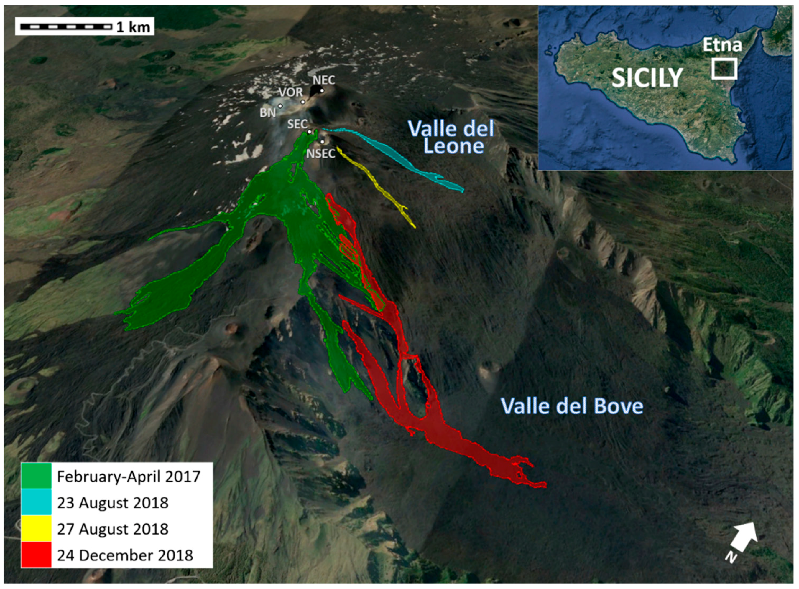
1.2. Recent Lava Flow-Forming Eruptions at Etna Volcano
2. Materials and Methods
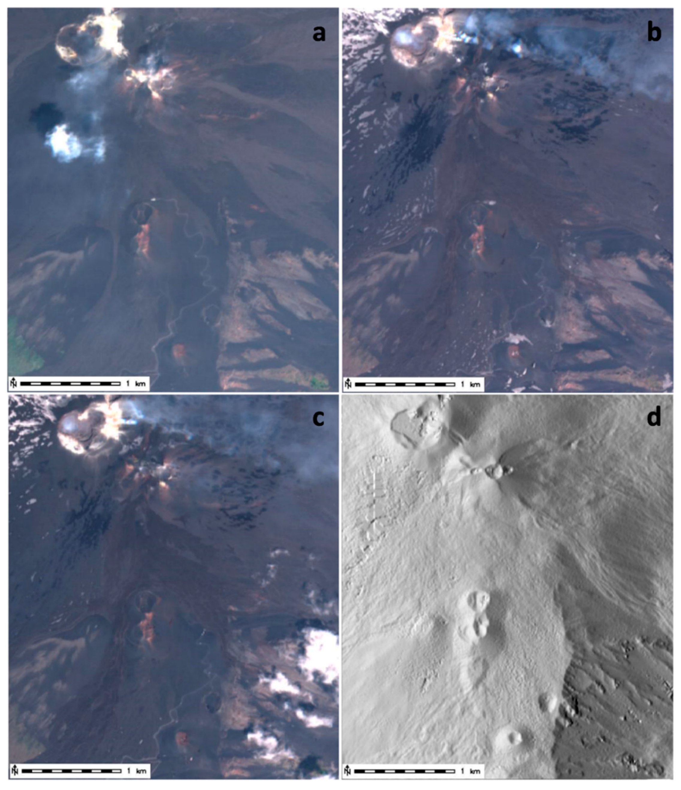
2.1. Data
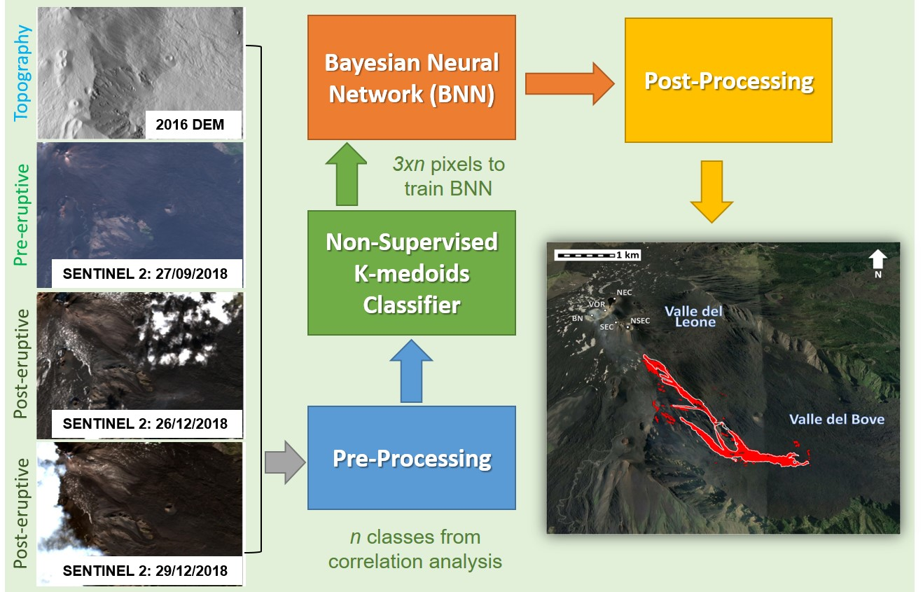
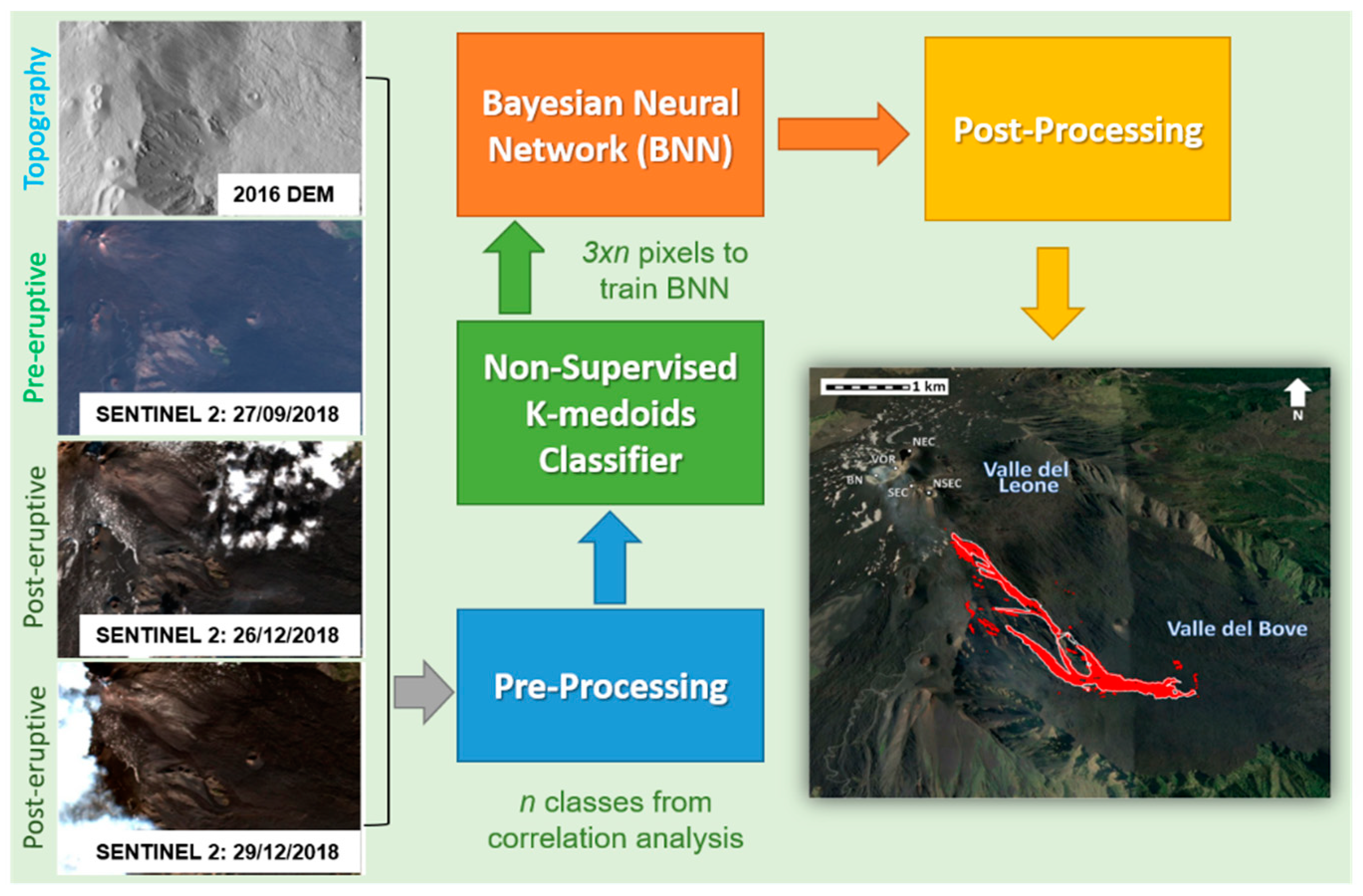
2.2. Workflow
3. Results
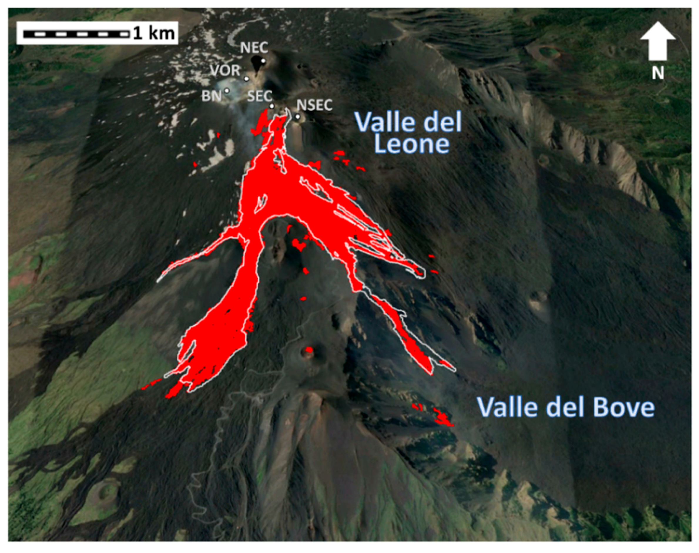
3.1. Case Study: February–April 2017
3.2. Case of Study: August 2018
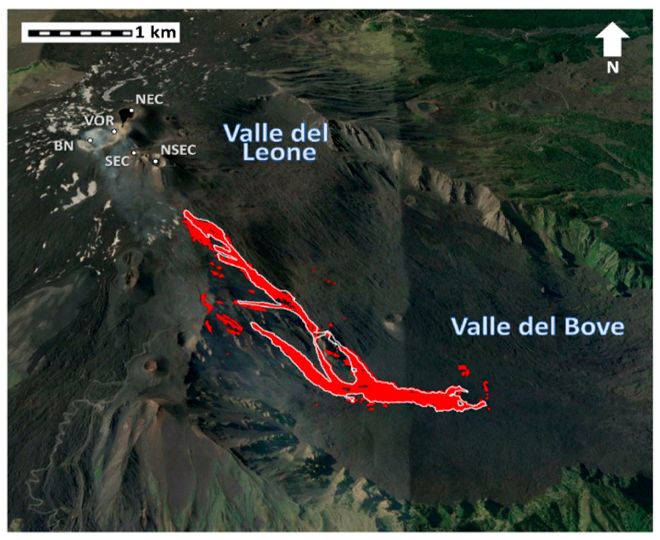
3.3. Case Study: December 2018
4. Discussion
- accuracy (ACC)
- precision (also known as the positive predictive value, PPV)
- sensitivity (also known as the true positive rate, TPR)
5. Conclusions
Author Contributions
Funding
Acknowledgments
Conflicts of Interest
References
- Del Negro, C.; Cappello, A.; Neri, M.; Bilotta, G.; Hérault, A.; Ganci, G. Etna flank lava flows between 1610 and 2008. PANGAEA 2013. [Google Scholar] [CrossRef]
- Cappello, A.; Geshi, N.; Neri, M.; Del Negro, C. Lava flow hazards-An impending threat at Miyakejima volcano, Japan. J. Volcanol. Geotherm. Res. 2015, 308, 1–9. [Google Scholar] [CrossRef]
- Cappello, A.; Zanon, V.; Del Negro, C.; Ferreira, T.J.L.; Queiroz, M.G.P.S. Exploring lava-flow hazards at Pico Island, Azores Archipelago (Portugal). Terra Nova 2015, 27, 156–161. [Google Scholar] [CrossRef]
- Pedrazzi, D.; Cappello, A.; Zanon, V.; Del Negro, C. Impact of effusive eruptions from the Eguas-Carvao fissure system, Sao Miguel Island, Azores Archipelago (Portugal). J. Volcanol. Geotherm. Res. 2015, 291, 1–13. [Google Scholar] [CrossRef]
- Pedersen, G.B.M.; Höskuldsson, A.; Dürig, T.; Thordarson, T.; Jónsdóttir, I.; Riishuus, M.S.; Óskarsson, B.V.; Dumont, S.; Magnusson, E.; Gudmundsson, M.T.; et al. Lava field evolution and emplacement dynamics of the 2014–2015 basaltic fissure eruption at Holuhraun, Iceland. J. Volcanol. Geotherm. Res. 2017, 340, 155–169. [Google Scholar] [CrossRef]
- Del Negro, C.; Cappello, A.; Ganci, G. Quantifying lava flow hazards in response to effusive eruption. Geol. Soc. Am. Bull. 2016, 128, 752–763. [Google Scholar] [CrossRef]
- Carr, B.B.; Clarke, A.B.; Arrowsmith, J.R.; Vanderkluysen, L.; Dhanu, B.E. The emplacement of the active lava flow at Sinabung Volcano, Sumatra, Indonesia, documented by structure-from-motion photogrammetry. J. Volcanol. Geotherm. Res. 2018. [Google Scholar] [CrossRef]
- James, M.R.; Pinkerton, H.; Applegarth, L.J. Detecting the development of active lava flow fields with a very-long-range terrestrial laser scanner and thermal imagery. Geophys. Res. Lett. 2009, 36, L22305. [Google Scholar] [CrossRef]
- James, M.R.; Pinkerton, H.; Robson, S. Image-based measurement of flux variation in distal regions of active lava flows. Geochem. Geophys. Geosyst. 2007, 8, Q03006. [Google Scholar] [CrossRef]
- Vicari, A.; Ganci, G.; Behncke, B.; Cappello, A.; Neri, M.; Del Negro, C. Near-real-time forecasting of lava flow hazards during the 12–13 January 2011 Etna eruption. Geophys. Res. Lett. 2011, 38, L13317. [Google Scholar] [CrossRef]
- Stevens, N.F.; Wadge, G.; Murray, J.B. Lava flow volume and morphology from digitised contour maps: A case study at Mount Etna, Sicily. Geomorphology 1999, 28, 251–261. [Google Scholar] [CrossRef]
- Cashman, K.V.; Sparks, R.S.J. How volcanoes work: A 25 year perspective. Geol. Soc. Am. Bull. 2013, 125, 664–690. [Google Scholar] [CrossRef]
- Turner, N.R.; Perroy, R.L.; Hon, K. Lava flow hazard prediction and monitoring with UAS: A case study from the 2014–2015 Pāhoa lava flow crisis, Hawai‘i. J. Appl. Volcanol. 2017, 6, 17. [Google Scholar] [CrossRef]
- Huang, H.; Long, J.; Yi, W.; Yi, Q.; Zhang, G.; Lei, B. Amethod for using unmanned aerial vehicles for emergency investigation of single geo-hazards and sample applications of this method. Nat. Hazards Earth Syst. Sci. 2017, 17, 1961–1979. [Google Scholar] [CrossRef]
- Ganci, G.; Cappello, A.; Bilotta, G.; Hérault, A.; Zago, V.; Del Negro, C. Mapping Volcanic Deposits of the 2011–2015 Etna Eruptive Events Using Satellite Remote Sensing. Front. Earth Sci. 2018, 6, 83. [Google Scholar] [CrossRef]
- Kauahikaua, J.; Margriter, S.; Lockwood, J.; Trusdell, F. Applications of GIS to the Estimation of Lava Flow Hazards on Mauna Loa Volcano, Hawai’I; Washington DC American Geophysical Union Geophysical Monograph; Series; American Geophysical Union: Washington, DC, USA, 1995; Volume 92, pp. 315–325. [Google Scholar]
- Calvari, S.; Neri, M.; Pinkerton, H. Effusion rate estimations during the 1999 summit eruption on Mount Etna, and growth of two distinct lava flow fields. J. Volcanol. Geotherm. Res. 2003, 119, 107–123. [Google Scholar] [CrossRef] [Green Version]
- Abrams, M.; Abbott, E.; Kahle, A. Combined use of visible, reflected infrared, and thermal infrared images for mapping Hawaiian lava flows. J. Geophys. Res. 1991, 96, 475–484. [Google Scholar] [CrossRef]
- Blackett, M. Review of the utility of infrared remote sensing for detecting and monitoring volcanic activity with the case study of shortwave infrared data for Lascar Volcano from 2001–2005. Geol. Soc. Lond. Spec. Publ. 2013, 380, 107–135. [Google Scholar] [CrossRef]
- Bonaccorso, A.; Caltabiano, T.; Currenti, G.; Del Negro, C.; Gambino, S.; Ganci, G.; Giammanco, S.; Greco, F.; Pistorio, A.; Salerno, G.; et al. Dynamics of a lava fountain revealed by geophysical, geochemical and thermal satellite measurements: The case of the 10 April 2011 Mt. Etna eruption. Geophys. Res. Lett. 2011, 38, L24307. [Google Scholar] [CrossRef]
- Kervyn, M.; Kervyn, F.; Goossens, R.; Rowland, S.K.; Ernst, G.G.J. Mapping volcanic terrain using high-resolution and 3D satellite remote sensing. Geol. Soc. Am. Bull. 2007, 283, 5–30. [Google Scholar] [CrossRef]
- Ganci, G.; Cappello, A.; Zago, V.; Bilotta, G.; Herault, A.; Del Negro, C. 3D Lava flow mapping of the 17-25 May 2016 Etna eruption using tri-stereo optical satellite data. Ann. Geophys. 2018. [Google Scholar] [CrossRef]
- Bonaccorso, A.; Calvari, S.; Currenti, G.; Del Negro, C.; Ganci, G.; Linde, A.; Napoli, R.; Sacks, S.; Sicali, A. From source to surface: Dynamics of Etna’s lava fountains investigated by continuous strain, magnetic, ground and satellite thermal data. Bull. Volcanol. 2013, 75, 690. [Google Scholar] [CrossRef]
- Amici, S.; Piscini, A.; Neri, M. Reflectance Spectra Measurements of Mt. Etna: A Comparison with Multispectral / Hyperspectral Satellite. Adv. Remote Sens. 2014, 3, 235–245. [Google Scholar] [CrossRef]
- Ganci, G.; Bilotta, G.; Cappello, A.; Herault, A.; Del Negro, C. HOTSAT: A multiplatform system for the thermal monitoring of volcanic activity using satellite data. Geolog. Soc. Lond. Spec. Publ. 2016, 426, 207–221. [Google Scholar] [CrossRef]
- Corradino, C.; Ganci, G.; Bilotta, G.; Cappello, A.; Del Negro, C.; Fortuna, L. Smart Decision Support Systems for Volcanic Applications. Energies 2019, 12, 1216. [Google Scholar] [CrossRef]
- Dietterich, H.R.; Downs, D.T.; Stelten, M.E.; Zahran, H. Reconstructing lava flow emplacement histories with rheological and morphological analyses: The Harrat Rahat volcanic field, Kingdom of Saudi Arabia. Bull. Volcanol. 2018, 80, 85. [Google Scholar] [CrossRef]
- Kubanek, J.; Richardson, J.A.; Charbonnier, S.J.; Connor, L.J. Lava flow mapping and volume calculations for the 2012–2013 Tolbachik, Kamchatka, fissure eruption using bistatic TanDEM-X InSAR. Bull. Volcanol. 2015, 77, 106. [Google Scholar] [CrossRef]
- Lu, Z.; Fielding, E.; Patrick, M.R.; Trautwein, C.M. Estimating lava volume by precision combination of multiple baseline spaceborne and airborne interferometric synthetic aperture radar: The 1997 eruption of Okmok volcano, Alaska. IEEE Trans. Geosci. Remote Sens. 2003, 41, 1428–1436. [Google Scholar] [CrossRef]
- Zebker, H.A.; Rosen, P.; Hensley, S.; Mouginis-Mark, P.J. Analysis of active lava flows on Kilauea volcano, Hawaii, using SIR-C radar correlation measurements. Geology 1996, 24, 495–498. [Google Scholar] [CrossRef]
- Dietterich, H.R.; Poland, M.P.; Schmidt, D.A.; Cashman, K.V.; Sherrod, D.R.; Espinosa, A.T. Tracking lava flow emplacement on the east rift zone of Kīlauea, Hawai’i, with synthetic aperture radar coherence. Geochem. Geoph. Geosy. 2012, 13. [Google Scholar] [CrossRef]
- Bonny, E.; Thordarson, T.; Wright, R.; Höskuldsson, A.; Jónsdóttir, I. The volume of lava erupted during the 2014 to 2015 eruption at Holuhraun, Iceland: A comparison between satellite- and ground-based measurements. J. Geophys. Res. Solid Earth 2018, 123, 5412–5426. [Google Scholar] [CrossRef]
- Head, E.M.; Maclean, A.L.; Carn, S.A. Mapping lava flows from Nyamuragira volcano (1967–2011) with satellite data and automated classification methods. Nat. Hazards Risk 2013, 4, 119–144. [Google Scholar] [CrossRef]
- Lu, Z.; Rykhus, R.; Masterlark, T.; Dean, K.G. Mapping recent lava flows at Westdahl Volcano, Alaska, using radar and optical satellite imagery. Remote Sens. Environ. 2004, 91, 345–353. [Google Scholar] [CrossRef]
- Bagnardi, M.; González, P.J.; Hooper, A. High-resolution digital elevation model from tri-stereo Pléiades-1 satellite imagery for lava flow volume estimates at Fogo Volcano. Geophys. Res. Lett. 2016, 43, 6267–6275. [Google Scholar] [CrossRef]
- Albino, F.; Smets, B.; d’Oreye, N.; Kervyn, F. High-resolution TanDEM-X DEM: An accurate method to estimate lava flow volumes at Nyamulagira volcano (D. R. Congo). J. Geophys. Res. Solid Earth 2015, 120, 4189–4207. [Google Scholar] [CrossRef]
- Anantrasirichai, N.; Achim, A.; Morgan, J.E.; Erchova, I.; Nicholson, L. SVM-based texture classification in optical coherence tomography. In Proceedings of the IEEE 10th International Symposium on Biomedical Imaging, San Francisco, CA, USA, 7–11 April 2013; pp. 1332–1335. [Google Scholar] [CrossRef]
- Anantrasirichai, N.; Biggs, J.; Albino, F.; Hill, P.; Bull, D. Application of Machine Learning to Classification of Volcanic Deformation in Routinely Generated InSAR Data. J. Geophys. Res. Solid Earth 2018, 123, 6592–6606. [Google Scholar] [CrossRef]
- Chang, N.B.; Bai, K.; Chen, C.F. Integrating multisensor satellite data merging and image reconstruction in support of machine learning for better water quality management. J. Environ. Manag. 2017, 201, 227–240. [Google Scholar] [CrossRef]
- Chang, C.C.; Lin, C.J. LIBSVM: A library for support vector machines. ACM Trans. Intell. Syst. Technol. 2011, 2, 27. [Google Scholar] [CrossRef]
- Jeppesen, J.H.; Jacobsen, R.H.; Inceoglu, F.; Toftegaard, T.S. A cloud detection algorithm for satellite imagery based on deep learning. Remote Sens. Environ. 2019, 229, 247–259. [Google Scholar] [CrossRef]
- Kotsiantis, S.B. Supervised machine learning: A review of classification techniques. In Emerging Artificial Intelligence Applications in Computer Engineering: Real Word AI Systems with Applications in eHealth, HCI, Information Retrieval and Pervasive Technologies; IOS Press: Amsterdam, The Netherlands, 2007; pp. 3–24. [Google Scholar]
- Yilmaz, I. Comparison of landslide susceptibility mapping methodologies for Koyulhisar, Turkey: Conditional probability, logistic regression, artificial neural networks, and support vector machine. Environ. Earth Sci. 2010, 61, 821–836. [Google Scholar] [CrossRef]
- Brown, M.; Lary, D.; Vrieling, A.; Stathakis, D.; Mussa, H. Neural networks as a tool for constructing continuous NDVI time series from AVHRR and MODIS. Int. J. Remote Sens. 2008, 29, 7141–7158. [Google Scholar] [CrossRef] [Green Version]
- Chen, Y.; Fan, R.; Bilal, M.; Yang, X.; Wang, J.; Li, W. Multilevel cloud detection for high-resolution remote sensing imagery using multiple convolutional neural networks. ISPRS Int. J. Geo Inf. 2018, 7, 181. [Google Scholar] [CrossRef]
- Kadavi, P.R.; Lee, C.W. Land cover classification analysis of volcanic island in Aleutian Arc using an artificial neural network (ANN) and a support vector machine (SVM) from Landsat imagery. Geosci. J. 2018, 22, 653–665. [Google Scholar] [CrossRef]
- Raith, S.; Vogel, E.P.; Anees, N.; Keul, C.; Güth, J.F.; Edelhoff, D.; Fischer, H. Artificial Neural Networks as a powerful numerical tool to classify specific features of a tooth based on 3D scan data. Comput. Biol. Med. 2017, 80, 65–76. [Google Scholar] [CrossRef] [PubMed]
- Apicella, M.L.; Buscarino, A.; Corradino, C.; Fortuna, L.; Mazzitelli, G.; Xibilia, M.G. Temperature Model Identification of FTU Liquid Lithium Limiter. IEEE Trans. Control Syst. Technol. 2018, 26, 1132–1139. [Google Scholar] [CrossRef]
- Yoshida, T.; Omatu, S. Pattern recognition with neural networks. In Proceedings of the IEEE 2000 International Geoscience and Remote Sensing Symposium. Taking the Pulse of the Planet: The Role of Remote Sensing in Managing the Environment Proceedings (Cat. No. 00CH37120), Honolulu, HI, USA, 24–28 July 2000; Volume 2, pp. 699–701. [Google Scholar]
- Adeli, H.; Panakkat, A. A probabilistic neural network for earthquake magnitude prediction. Neural Netw. 2009, 22, 1018–1024. [Google Scholar] [CrossRef] [PubMed]
- Erhan, D.; Bengio, Y.; Courville, A.; Manzagol, P.A.; Vincent, P.; Bengio, S. Why does unsupervised pre-training help deep learning? J. Mach. Learn. Res. 2010, 11, 625–660. [Google Scholar]
- Gaddam, S.R.; Phoha, V.V.; Balagani, K.S. K-Means+ID3: A novel method for supervised anomaly detection by cascading K-Means clustering and ID3 decision tree learning methods. IEEE Trans. Knowl. Data Eng. 2007, 19, 345–354. [Google Scholar] [CrossRef]
- Tien Bui, D.; Tuan, T.A.; Hoang, N.D.; Thanh, N.Q.; Nguyen, D.B.; Van Liem, N.; Pradhan, B. Spatial prediction of rainfall-induced landslides for the Lao Cai area (Vietnam) using a hybrid intelligent approach of least squares support vector machines inference model and artificial bee colony optimization. Landslides 2017, 14, 447–458. [Google Scholar] [CrossRef]
- Handayani, A.N.; Lathifah, N.; Herwanto, H.W.; Asmara, R.S.; Arai, K. Neural Network Bayesian Regularization Backpropagation to Solve Inverse Kinematics on Planar Manipulator. In Proceedings of the 2018 Joint 7th International Conference on Informatics, Electronics & Vision (ICIEV) and 2018 2nd International Conference on Imaging, Vision & Pattern Recognition (ICIVPR), Kitakyushu, Japan, 25–29 June 2018; pp. 99–104. [Google Scholar]
- Cappello, A.; Bilotta, G.; Neri, M.; Del Negro, C. Probabilistic modeling of future volcanic eruptions at Mount Etna. J. Geophys. Res. Solid Earth 2013, 118, 1925–1935. [Google Scholar] [CrossRef] [Green Version]
- Acocella, V.; Neri, M.; Behncke, B.; Bonforte, A.; Del Negro, C.; Ganci, G. Why does a mature volcano need new vents? the case of the new southeast crater at etna. Front. Earth Sci. 2016, 4, 67. [Google Scholar] [CrossRef]
- Neri, M.; Acocella, V.; Behncke, B.; Maiolino, V.; Ursino, A.; Velardita, R. Contrasting triggering mechanisms of the 2001 and 2002–2003 eruptions of Mount Etna (Italy). J. Volcanol. Geotherm. Res. 2005, 144, 235–255. [Google Scholar] [CrossRef]
- Behncke, B.; Fornaciai, A.; Neri, M.; Favalli, M.; Ganci, G.; Mazzarini, F. Lidar surveys reveal eruptive volumes and rates at Etna, 2007–2010. Geophys. Res. Lett. 2016, 43, 4270–4278. [Google Scholar] [CrossRef]
- Ganci, G.; Vicari, A.; Cappello, A.; Del Negro, C. An emergent strategy for volcano hazard assessment: From thermal satellite monitoring to lava flow modeling. Remote Sens. Environ. 2012, 119, 197–207. [Google Scholar] [CrossRef]
- Ganci, G.; Cappello, A.; Bilotta, G.; Corradino, C.; Del Negro, C. Satellite-Based Reconstruction of the Volcanic Deposits during the December 2015 Etna Eruption. Data 2019, 4, 120. [Google Scholar] [CrossRef]
- Cappello, A.; Ganci, G.; Bilotta, G.; Corradino, C.; Herault, A.; Del Negro, C. Changing eruptive styles at the South-East Crater of Mount Etna: Implications for assessing lava flow hazards. Front. Earth Sci. 2019, 7, 213. [Google Scholar] [CrossRef]
- Del Negro, C.; Cappello, A.; Neri, M.; Bilotta, G.; Herault, A.; Ganci, G. Lava flow hazards at Mount Etna: Constraints imposed by eruptive history and numerical simulations. Sci. Rep. 2013, 3, 3493. [Google Scholar] [CrossRef]
- Patrick, M.R.; Dehn, J.; Papp, K.R.; Lu, Z.; Dean, K.; Moxey, L.; Izbekov, P.; Guritz, R. The 1997 eruption of Okmok Volcano, Alaska: A synthesis of remotely sensed imagery. J. Volcanol. Geoth. Res. 2003, 127, 87–105. [Google Scholar] [CrossRef]
- Pyle, D.M.; Mather, T.A.; Biggs, J. Remote sensing of volcanoes and volcanic processes: Integrating observation and modelling–introduction. Geol. Soc. Lond. Spec. Publ. 2013, 380, 1–13. [Google Scholar] [CrossRef]
- Rogic, N.; Cappello, A.; Ferrucci, F. Role of Emissivity in Lava Flow ‘Distance-to-Run’ Estimates from Satellite-Based Volcano Monitoring. Remote Sens. 2019, 11, 662. [Google Scholar] [CrossRef]
- Valade, S.; Ley, A.; Massimetti, F.; D’Hondt, O.; Laiolo, M.; Coppola, D.; Loibl, D.; Hellwich, O.; Walter, T.R. Towards Global Volcano Monitoring Using Multisensor Sentinel Missions and Artificial Intelligence: The MOUNTS Monitoring System. Remote Sens. 2019, 11, 1528. [Google Scholar] [CrossRef]
- Wadge, G. A strategy for the observation of volcanism on Earth from space. Philos. Trans. R. Soc. Lond. Ser. A Math. Phys. Sci. 2003, 361, 145–156. [Google Scholar] [CrossRef] [PubMed]
- Aufaristama, M.; Hoskuldsson, A.; Jonsdottir, I.; Ulfarsson, M.; Thordarson, T. New Insights for Detecting and Deriving Thermal Properties of Lava Flow Using Infrared Satellite during 2014–2015 Effusive Eruption at Holuhraun, Iceland. Remote Sens. 2018, 10, 151. [Google Scholar] [CrossRef]
- Camacho-Alpízar, A.; Fuchs, E.J.; Barrantes, G. Effect of barriers and distance on song, genetic, and morphological divergence in the highland endemic Timberline Wren (Thryorchilus browni, Troglodytidae). PLoS ONE 2018, 13, e0209508. [Google Scholar] [CrossRef]
- Aufaristama, M.; Hoskuldsson, A.; Ulfarsson, M.O.; Jonsdottir, I.; Thordarson, T. The 2014–2015 Lava Flow Field at Holuhraun, Iceland: Using Airborne Hyperspectral Remote Sensing for Discriminating the Lava Surface. Remote Sens. 2019, 11, 476. [Google Scholar] [CrossRef]
- Li, L.; Solana, C.; Canters, F.; Kervyn, M. Testing random forest classification for identifying lava flows and mapping age groups on a single Landsat 8 image. J. Volcanol. Geotherm. Res. 2017, 345, 109–124. [Google Scholar] [CrossRef] [Green Version]
- Spinetti, C.; Mazzarini, F.; Casacchia, R.; Colini, L.; Neri, M.; Behncke, B.; Salvatori, R.; Buongiorno, M.F.; Pareschi, M.T. Spectral properties of volcanic materials from hyperspectral field and satellite data compared with LiDAR data at Mt. Etna. Int. J. Appl. Earth Obs. Geoinf. 2009, 11, 142–155. [Google Scholar] [CrossRef]
- Lary, D.J.; Alavi, A.H.; Gandomi, A.H.; Walker, A.L. Machine learning in geosciences and remote sensing. Geosci. Front. 2016, 7, 3–10. [Google Scholar] [CrossRef] [Green Version]
- Li, C.; Wang, J.; Wang, L.; Hu, L.; Gong, P. Comparison of classification algorithms and training sample sizes in urban land classification with Landsat thematic mapper imagery. Remote Sens. 2014, 6, 964–983. [Google Scholar] [CrossRef]
- Lüdtke, A.; Jerosch, K.; Herzog, O.; Schlüter, M. Development of a machine learning technique for automatic analysis of seafloor image data: Case example, Pogonophora coverage at mud volcanoes. Comput. Geosci. 2012, 39, 120–128. [Google Scholar] [CrossRef] [Green Version]
- Ganci, G.; Cappello, A.; Bilotta, G.; Hérault, A.; Zago, V.; Del Negro, C. 3D Lava flow mapping at Etna volcano from Pléiades-derived DEM differences. PANGAEA 2019. [Google Scholar] [CrossRef]
- Jain, A.K.; Dubes, R.C. Algorithms for Clustering Data; Prentice Hall: Englewood Cliffs, NJ, USA, 1988; Volume 6. [Google Scholar]
- Christopher, B. Pattern Recognition and Machine Learning; Springer: Berlin/Heidelberg, Germany, 2006. [Google Scholar]
- Cappello, A.; Ganci, G.; Bilotta, G.; Herault, A.; Zago, V.; Del Negro, C. Satellite-driven modeling approach for monitoring lava flow hazards during the 2017 Etna eruption. Ann. Geophys. 2018, 61, 13. [Google Scholar] [CrossRef]
- Kereszturi, G.; Cappello, A.; Ganci, G.; Procter, J.; Németh, K.; Del Negro, C.; Cronin, S.J. Numerical simulation of basaltic lava flows in the Auckland Volcanic Field, New Zealand – Implication for volcanic hazard assessment. Bull. Volcanol. 2014, 76, 879. [Google Scholar] [CrossRef]
- Kereszturi, G.; Nemeth, K.; Vioufti, M.R.; Cappello, A.; Murcia, H.; Ganci, G.; Del Negro, C.; Procter, J.; Zahran, H.M.A. Emplacement conditions of the 1256 AD Al-Madinah lava flow field in Harrat Rahat, Kingdom of Saudi Arabia—Insights from surface morphology and lava flow simulations. J. Volcanol. Geotherm. Res. 2016, 309, 14–30. [Google Scholar] [CrossRef]
- Cappello, A.; Ganci, G.; Calvari, S.; Perez, N.M.; Hernandez, P.A.; Silva, S.V.; Cabral, J.; Del Negro, C. Lava flow hazard modeling during the 2014–2015 Fogo eruption, Cape Verde. J. Geophys. Res. Solid Earth 2016, 121, 2290–2303. [Google Scholar] [CrossRef]
- Bilotta, G.; Cappello, A.; Hérault, A.; Vicari, A.; Russo, G.; Del Negro, C. Sensitivity analysis of the MAGFLOW Cellular Automaton model for lava flow simulation. Environ. Model. Softw. 2012, 35, 122–131. [Google Scholar] [CrossRef]
- Bilotta, G.; Cappello, A.; Hérault, A.; Del Negro, C. Influence of topographic data uncertainties and model resolution on the numerical simulation of lava flows. Environ. Model. Softw. 2019, 112, 1–15. [Google Scholar] [CrossRef]
- Aufaristama, M.; Höskuldsson, Á.; Jónsdóttir, I.; Ólafsdóttir, R. Mapping and Assessing Surface Morphology of Holocene Lava Field in Krafla (NE Iceland) Using Hyperspectral Remote Sensing. IOP Conf. Ser. Earth Environ. Sci. 2016, 29, 1–6. [Google Scholar] [CrossRef]
- Bailey, J.E.; Harris, A.J.L.; Dehn, J.; Calvari, S.; Rowland, S.K. The changing morphology of an open lava channel on Mt. Etna. Bull. Volcanol. 2006, 68, 497–515. [Google Scholar] [CrossRef] [Green Version]
- Kolzenburg, S.; Jaenicke, J.; Münzer, U.; Dingwell, D.B. The effect of inflation on the morphology-derived rheological parameters of lava flows and its implications for interpreting remote sensing data—A case study on the 2014/2015 eruption at Holuhraun, Iceland. J. Volcanol. Geotherm. Res. 2018, 357, 200–212. [Google Scholar] [CrossRef]
- Pinkerton, H.; James, M.; Jones, A. Surface temperature measurements of active lava flows on Kilauea volcano, Hawai’i. J. Volcanol. Geotherm. Res. 2002, 113, 159–176. [Google Scholar] [CrossRef]


| Eruption Date | Area [km2] | ACC | PPV | TPR | |||||
|---|---|---|---|---|---|---|---|---|---|
| REAL | BNN | GROUND | BNN | GROUND | BNN | GROUND | BNN | GROUND | |
| February–April 2017 | 2.03 | 1.99 | 1.45 | 0.88 | 0.73 | 0.88 | 0.83 | 0.86 | 0.60 |
| August 2018 | 0.21 | 0.28 | 0.38 | 0.73 | 0.52 | 0.60 | 0.33 | 0.81 | 0.58 |
| December 2018 | 0.88 | 0.94 | 0.73 | 0.83 | 0.58 | 0.79 | 0.56 | 0.84 | 0.46 |
© 2019 by the authors. Licensee MDPI, Basel, Switzerland. This article is an open access article distributed under the terms and conditions of the Creative Commons Attribution (CC BY) license (http://creativecommons.org/licenses/by/4.0/).
Share and Cite
Corradino, C.; Ganci, G.; Cappello, A.; Bilotta, G.; Hérault, A.; Del Negro, C. Mapping Recent Lava Flows at Mount Etna Using Multispectral Sentinel-2 Images and Machine Learning Techniques. Remote Sens. 2019, 11, 1916. https://0-doi-org.brum.beds.ac.uk/10.3390/rs11161916
Corradino C, Ganci G, Cappello A, Bilotta G, Hérault A, Del Negro C. Mapping Recent Lava Flows at Mount Etna Using Multispectral Sentinel-2 Images and Machine Learning Techniques. Remote Sensing. 2019; 11(16):1916. https://0-doi-org.brum.beds.ac.uk/10.3390/rs11161916
Chicago/Turabian StyleCorradino, Claudia, Gaetana Ganci, Annalisa Cappello, Giuseppe Bilotta, Alexis Hérault, and Ciro Del Negro. 2019. "Mapping Recent Lava Flows at Mount Etna Using Multispectral Sentinel-2 Images and Machine Learning Techniques" Remote Sensing 11, no. 16: 1916. https://0-doi-org.brum.beds.ac.uk/10.3390/rs11161916