Super-Resolved Multiple Scatterers Detection in SAR Tomography Based on Compressive Sensing Generalized Likelihood Ratio Test (CS-GLRT)

Abstract

The application of SAR tomography (TomoSAR) on the urban infrastructure and other man-made buildings has gained increasing popularity with the development of modern high-resolution spaceborne satellites. Urban tomography focuses on the separation of the overlaid targets within one azimuth-range resolution cell, and on the reconstruction of their reflectivity profiles. In this work, we build on the existing methods of compressive sensing (CS) and generalized likelihood ratio test (GLRT), and develop a multiple scatterers detection method named CS-GLRT to automatically recognize the number of scatterers superimposed within a single pixel as well as to reconstruct the backscattered reflectivity profiles of the detected scatterers. The proposed CS-GLRT adopts a two-step strategy. In the first step, an L1-norm minimization is carried out to give a robust estimation of the candidate positions pixel by pixel with super-resolution. In the second step, a multiple hypothesis test is implemented in the GLRT to achieve model order selection, where the mapping matrix is constrained within the afore-selected columns, namely, within the candidate positions, and the parameters are estimated by least square (LS) method. Numerical experiments on simulated data were carried out, and the presented results show its capability of separating the closely located scatterers with a quasi-constant false alarm rate (QCFAR), as well as of obtaining an estimation accuracy approaching the Cramer–Rao Low Bound (CRLB). Experiments on real data of Spotlight TerraSAR-X show that CS-GLRT allows detecting single scatterers with high density, distinguishing a considerable number of double scatterers, and even detecting triple scatterers. The estimated results agree well with the ground truth and help interpret the true structure of the complex or buildings studied in the SAR images. It should be noted that this method is especially suitable for urban areas with very dense infrastructure and man-made buildings, and for datasets with tightly-controlled baseline distribution.

1. Introduction

Synthetic aperture radar tomography (TomoSAR) [1] has successfully been used to reconstruct three-dimensional (3D) urban infrastructures [2,3], to estimate the forest biomass [4,5], and to image ice structures [6,7]. The launch of the new generation of spaceborne satellites (e.g., TerraSAR-X/Tan-DEM-X, COSMO-SkyMed, and Gaofen-3) provides SAR images with unprecedented high resolution up to meter regime and even to submeter regime, which dramatically facilitates the reconstruction and monitoring of urban infrastructures.

The TomoSAR reconstruction can be regarded as an inverse problem, which was firstly solved by the nonparametric methods such as beamforming (BF) [1,8], singular value decomposition (SVD) [9,10], and adaptive Capon [11,12,13]. BF and SVD get their popularity from their high efficiency and robustness. Both methods can preserve the full resolution of SAR images, but suffer from low resolution and high side-lobe level problems. Capon allows super-resolution imaging at the expense of a spatial resolution loss as multi-look processing is required. Parametric methods, such as multiple signal classification (MUSIC) [14], have also been introduced for TomoSAR. MUSIC can achieve super-resolution and side-lobe reduction but it requires a priori information and is sensitive to model errors. Based on the fact that target distribution along elevation is always sparse, especially in urban areas, compressive sensing (CS) [15,16,17] provides another solution for infrastructure tomographic reconstruction. It enhances the elevation resolution within the single-look archive and reduces the required number of measurements, while its main limitations stem from the off-grid effect so as to generate spurious outliers, the amplitude bias, and the inability to evaluate the probability of detection and the probability of false alarm.

While these methods provide the foundations for significant advances, technical issues of the exact number of targets or scatterers remain to be decided when applied in urban scene study. Automatic methods for detection and reconstruction of infrastructure and other man-made structures in urban area have been widely studied. According to the different methods of model order selection (MOS), existing methods can be classified into three groups: the generalized likelihood ratio test (GLRT) based [18,19,20,21,22,23,24]; information criterion based, such as Bayes information criterion (BIC) and Akaike information criterion (AIC) [25,26,27]; and no additional MOS based or iterative reweighted method [28,29,30].

An approach based on GLRT for the detection of targets in the tomographic framework was proposed in [18] (BF based GLRT) for the first time. As an extension of the work in [18], an approach focusing on the discrimination of single and double scatterers was introduced [19]. It could effectively estimate the positions and number of scatterers with constant false alarm rate (CFAR) efficiently. However, it suffered from the leakage effects related to side-lobe influence and from a low intrinsic elevation resolution, the so-called Rayleigh resolution. Rayleigh resolution is inversely proportional to the perpendicular baseline extension and is typically much worse than the resolution in azimuth and range, which makes it far from satisfactory when applied in the urban areas with high resolution and tightly-controlled TerraSAR/TanDEM-X. A support GLRT (sup-GLRT) method [20] was proposed to deal with the poor elevation resolution problem. It searches the best signal support to decide the number and positions of the significant scatterers based on nonlinear maximum for detecting at most $K_{max}$ scatterers. It is convenient when the scatterer distribution is very sparse (no more than two), while the computing complexity will increase dramatically with the increase of $K_{max}$. To mitigate the computational burden, a fast sup-GLRT method [21], referred to as M-sup-GLRT, was proposed. It transfers the multidimensional optimal searching problem into a $K_{max}$ 1D optimal searching one, so as to enjoy the computational efficiency as well a super-resolution capability comparable to that of sup-GLRT. Most recently, M-sup-GLRT has been extended to 5D application [22] and showed the ability to not only monitor temporal deformation but also to detect the thermal dilation. Another application of sup-GLRT is the investigation of polarimetric TomoSAR (Pol-TomoSAR), which allows the reduction of the number of acquisitions required. Multilook GLRT, referred to as M-GLRT has been proposed to improve the detection capability over man-made targets as well in areas characterized by low SNRs [23]. As an extension of the method in [23], the Capon filter has been introduced in M-GLRT [24] to get a super-resolution ability.

SL1MMER [25,26] has been proposed to eliminate the outliers and get the accurate parameter estimation by introducing two steps of BIC MOS and parameter estimation. It can effectively drop the outliers by penalizing the higher orders and estimating the parameters by scale down L2 method. SL1MMER is super-resolved and has been proven perfect for the urban reconstruction [25,26]. Most recently, integrating with geographic information systems (GIS), its extended version, M-SL1MMER [31], has been proven to have an accurate tomographic reconstruction capability with even very small images. However, it greatly depends on the penalized parameters and there is no effective way to evaluate the false alarm rate, or it is not a CFAR estimation. A nonparametric iterative adaptive approach (IAA) [27] combined with an MOS of BIC, referred to as IAA-BIC, has been proposed to retrieve 3D structure infrastructures. It does not require any a priori knowledge or hyperparameter selection, and it performed well for both distributed and coherent scatterers with either a few multiple looks or single-look. However, when applied to the single-look urban study, the weighted matrix, corresponding to the inversion of data covariance matrix, is not always invertible.

An iterative reweighted CS (IR-CS) [28] method has been proposed to eliminate the spurious outliers by iterative reweighted L1 minimization. The outliers can be dropped effectively, especially at low SNR cases with doubling or tripling the calculation complexity. Another IR method called iterative reweighted alternating direction method of multipliers (IR-ADMM) [29] has been proposed to relieve the computational burden with almost the same elevation accuracy and with only a slightly worse detection rate than that of IR-CS. A two-step iterative shrinkage/thresholding (TWIST) [30] approach for TomoSAR was proposed to speed up the L1-Norm minimization procedure as well as to achieve unbiased estimation for ill-conditioned problem.

In this paper, we aim at proposing a multiple scatterers detection method in tomography with the following characteristics: (1) CFAR or quasi-CFAR; (2) super resolution capability; (3) high detection probability; (4) accurate elevation estimation; (5) full spatial resolution; and (6) acceptable computing complexity even with the increase of model order. To these ends, an approach named CS-GLRT is proposed by a two-step processing method. Firstly, a scale down support space is obtained by CS so as to super-resolve the problem as well as to provide a priori information for the next step about the candidate positions. Then, within the scaled down space, optimal research is implemented for each model order, followed by a $K+1$-order hypothesis test, where each hypothesis test is conducted in a GLRT archive. The first step gives the potential positions, with which the computing complexity is greatly reduced for the second step’s optimal research. The second step separates the closely located scatterers without setting any hyperparameters with the false alarm rate (FAR) being controlled. The proposed approach is robustly applicable to triple or even higher order scatterers detection without much computational burden increase. The effectiveness was validated by simulated data as well by real data of TerraSAR-X spotlight over Shenzhen, China. Simulated results show that the proposed method can robustly super-resolve the overlaid targets with an accuracy approaching the Cramer–Rao Low Bound ($CRLB$). Real-data results show its capability of detecting single scatterers with high density, distinguishing a considerable number of double scatterers, and even detecting triple scatterers, whose results are consistent with the ground truth. In addition, comparisons of CS-GLRT and SL1MMER on false detection rate, and of CS-GLRT and sup-GLRT on computational burden were carried out. The results imply that CS-GLRT provides an alternative for SL1MMER and for sup-GLRT as it is a good tradeoff for robustness and efficiency. It should be noted that, to realize the sparse reconstruction, an open source software package named SparseLab [32] is used.

This paper is organized as follows. In Section 2, the signal model of TomoSAR and procedures of GLRT are reviewed. Section 3 explains the theoretical basis of CS and gives the proposed CS-GLRT methodology. Section 4 and Section 5 are devoted to the simulated and real data experiments, respectively. Section 6 addresses the additional discussions and comparisons. Finally, Section 7 gives the conclusion.

2. Signal Model and Problem Formulation TomoSAR

2.1. Acquisition Model

TomoSAR utilizes the multi-baseline sensors aligned along the elevation s over the same area, with slightly different view angles, allowing the capability to fully image the scene in the 3D space, whose imaging geometry is shown in Figure 1. Each azimuth-range pixel collects a stack of N focused images coregistered with respect to a given (master) one,

$$g_n=\int \gamma \left(s\right)exp(-j2\pi {\xi }_{n}s)ds,n=1,...,N$$

(1)

where $\gamma \left(s\right)$ is the reflectivity function along elevation, and ${\xi }_n=-{\displaystyle \frac{2b_{\perp n}}{\lambda r}}$ denotes the spatial frequency with $b_{\perp n}$ being the perpendicular baseline relative to the master sensor, $\lambda$ representing the wavelength, and r being the slant range distance. Approximately discretizing the continuous reflectivity function along s and considering the noise in the real scenario, Equation (1) can be rewritten as

$$\mathbf{g}=\mathbf{L}\gamma +\mathbf{w},$$

(2)

where $\mathbf{L}$ is the steering matrix mapping the model space into the data space, with the generic element expressed as,

$${\ell }_i={\left[exp\{-j2\pi {\xi }_1{s}_i\},exp\{-j2\pi {\xi }_2{s}_i\},...,exp\{-j2\pi {\xi }_N{s}_i\}\right]}^T,$$

(3)

and $\mathbf{w}$ is the N-dimensional noise vector, circular Gaussian distributed with zero mean and a covariance matrix of ${\sigma }^2{\mathbf{I}}_N$, where ${\sigma }^2$ is the noise power and ${\mathbf{I}}_N$ denotes the $N\times N$ identity matrix. The straightforward solution of Equation (2) is the so-called BF or periodogram,

$$\stackrel{⌢}{\gamma }={\mathbf{L}}^H\mathbf{g},$$

(4)

where ${(•)}^H$ denotes the Hermitian operation.

For urban study, one important application is separating multiple scatters interfering within the same range-azimuth resolution cell, or layover mechanism separation, as shown in Figure 1 by red and blue dots. BF as well as other nonparametric imaging methods is limited by the grating lobes caused by the nonuniform distribution of the baselines, and also by the low Rayleigh resolution inversely proportional to the perpendicular baseline extension,

$${\rho }_s=\frac{\lambda r}{2B_{\perp }},$$

(5)

where $B_{\perp }$ is the perpendicular baseline extension. For the modern TerraSAR-X/TanDEM-X spaceborne mission, whose baseline is strictly controlled within 400–500 m, leading to a common ${\rho }_s$ of 20–30 m, which is typically only $\frac{1}{30}$–$\frac{1}{20}$ of the resolution in range and azimuth. When dealing with the superposition of scatterers from building facade/roof and the ground, the 20–30 m resolution is far from satisfactory, leading to the desperate demand for imaging methods with super-resolution capability. Actually, for single scatterer detection, there is a $CRLB$ for elevation (see the detailed deduction in Appendix A.1), expressed as

$${\sigma }_s=\frac{\lambda r}{4\pi \sqrt{2N•SNR}•{\sigma }_b},$$

(6)

where $SNR$ is the signal-to-noise ratio and ${\sigma }_b$ is the standard deviation of the spatial baseline. Using the parameters of TerraSAR-X (see

Table 1. Parameters of TerraSAR-X.

Symbol	Description	Values
$R_0$	Sensor-to-target distance	645,639 m
f	Operating frequency	9.65 GHz
$\theta$	Local incidence angle	${39.5}^{\circ }$

for systematic parameters and Figure 2 for baseline distribution, respectively), if $SNR=10$ dB (a common SNR for permanent scatterers (PS)), ${\sigma }_s=0.68$ m can be obtained. Usually, for an unbiased estimation, whose error can be controlled within $\pm CRLB$, it can be considered as an excellent estimator [33]. It should be noted that, if there are no targets located less than ${\rho }_s$, BF or unmodified periodogram turns out to be the excellent estimator which outperforms any of the super-resolution methods [33].

2.2. Problem Formulation

GLRT’s first introduction to TomoSAR was devoted to deciding the presence or absence of a single target by a binary hypothesis test [18], with $H_i$ denoting the different hypotheses

H_i: presence of i target with i = 0, 1

and $D_i$ representing the decision, whose decision rule is

$$F\left(\mathbf{g}\right)=\frac{\underset{\gamma ,{\sigma }^2}{max}p(\mathbf{g};\gamma ,{\sigma }^2,H_1)}{\underset{{\sigma }^2}{max}p(\mathbf{g};{\sigma }^2,H_0)}{\displaystyle \underset{D_0}{\overset{D_1}{\gtrless }}}T,$$

(7)

where $p(\mathbf{g};\gamma ,{\sigma }^2,H_1)$ and $p(\mathbf{g};{\sigma }^2,H_0)$ are the likelihood functions of $\mathbf{g}$ under $H_1$ and $H_0$, respectively, and T is the decision threshold, which is set according to the desired value of false alarm probability $P_{fa}$ (which is defined in Section 3).

In the problem under study, we are interested in estimating, pixel by pixel, the number of scatterers k superimposed in a single pixel and the corresponding parameter vectors, i.e., magnitude, elevation and phase. Moreover, a maximum sparseness of K is assumed in the elevation direction, and it is convenient to cast the problem in terms of multiple statistical hypothesis testing with the signal model written as

$$\begin{array}{c}{H}_0:\mathbf{g}=\mathbf{w}\hfill \\ H_k:\mathbf{g}={\displaystyle \sum _{i=1}^k}{\gamma }_{i}l\left(s_i\right)+\mathbf{w},k=1,2,...,K\hfill \end{array}$$

(8)

which can be solved in the framework of the detection theory. It consists of $K+1$ steps where binary tests are sequentially applied in each step, as shown in Figure 3, with $F_i$ and $T_i$ being the general likelihood ratio and the decision threshold for the ith step, respectively ($F_i$ and $T_i$ are both given in the next section).

3. Problem Solution

3.1. CS

Based on the assumption that only a low number of scatterers with different elevations are present in the same range-azimuth resolution cell, CS, a popular approach for sparse signal reconstruction method, provides a new sampling theory for data acquisition and allows super-resolution using only few signal samples. It has been proven perfectly suitable for urban tomographic reconstruction [15,16]. The sparse theory says that, when the restricted isometry property (RIP) (see Equation (15)) and the incoherence property are met, K-sparse signal $\gamma$ can be exactly recovered by L1 minimization as

$$\stackrel{⌢}{\gamma }=\arg \underset{\gamma }{\min }\{\parallel g-\mathbf{\Phi }{\parallel }_2^2+{\lambda }_K\parallel \lambda \parallel {}_1\}$$

(9)

where ${\lambda }_K$ denotes the Lagrange multiplier depending on the number of samples N and the noise level [34]. $\Phi$ is the normalized version of $\mathbf{L}$, i.e., $\Phi =\frac{\mathbf{L}}{\sqrt{N}}$. The ${\ell }_2$ -term ${∥•∥}_2^2$ forces the residual $\mathbf{g}-\mathbf{L}\gamma$ to be small, whereas the ${\ell }_1$-term ${∥•∥}_1$ enforces the sparsity of the representation. ${\lambda }_K$ controls the tradeoff between the sparsity of the spectrum and the residual norm. According to [34], if the dictionary is an orthogonal basis, the mean-squared error properties are near optimal if we set $\lambda$ as ${\lambda }_K={\sigma }_{\epsilon }\sqrt{2log\left(N\right)}$. The readers can refer to Appendix A.2 for more details about the deviation of ${\lambda }_K$. Here, ${\sigma }_{\epsilon }$ is the noise level, which can be estimated using several methods, e.g., SVD-Wiener [35]. According to Equation (8), in both simulations and real-data experiments, ${\sigma }_{\epsilon }$ can be simply estimated as ${\sigma }_{\epsilon }=\sqrt{E\left(\mathbf{g}{\mathbf{g}}^{\mathbf{T}}\right)-{\left(E\right(\left|\mathbf{g}\right|\left)\right)}^2}$, where $E\left(•\right)$ means the expectation operation. With CS applied in SAR tomography, super resolution capability as well as robustness to phase noise can be obtained. Nevertheless, as the RIP and incoherence property are often violated because of the predefined $\mathbf{L}$, the over-sampling rate along elevation and so on, spurious artifacts often exist.

3.2. CS-GLRT

Before describing the proposed method, here, some shortcomings of CS and the BF based GLRT are listed, respectively, as follows:

• CS
  • Spurious artifacts
  • Underestimation of magnitude
• BF based GLRT
  • Low resolution
  • Side-lobe effect

X.X. Zhu [25] and A. Budillon [20] have already dedicated to circumventing the mentioned limitations referred to as SL1MMER and sup-GLRT, respectively. As we know, the limitations of CS stem from the magnitude being underestimated and there being outliers around the true position of targets. However, it can be believed that the correct positions can always be detected despite the outliers and underestimated magnitude. Assume that there are up to K scatterers superimposed within a single pixel; it is reasonable to set $K_{max}=3K$ potential positions, considering two outliers around each true position. With these $K_{max}$ candidate positions, we can greatly scale down the steering matrix $\mathbf{L}$ to a $K_{max}$-column mapping matrix ${\mathbf{L}}^{\prime }$. Then, following the guidelines of [20], we can apply GLRT with $K_{max}$-column ${\mathbf{L}}^{\prime }$ rather than with M-column $\mathbf{L}$. In our multiple scatterers case, the decision rule in Equation (7) can then be expressed as

$$F_i\left(\mathbf{g}\right)=\frac{\underset{{\gamma }_{{\Omega }_j},{\Omega }_j,{\sigma }^2}{max}p(\mathbf{g};{\gamma }_{{\Omega }_j},{\Omega }_j,{\sigma }^2,H_j)}{\underset{{\gamma }_{{\Omega }_{i-1}},{\Omega }_{i-1},{\sigma }^2}{max}p(\mathbf{g};{\gamma }_{{\Omega }_{i-1}},{\Omega }_{i-1},{\sigma }^2,H_{i-1})}{\displaystyle \underset{D_{i-1}}{\overset{D_{k⩾i}}{\gtrless }}}{T}_i,j=i,...,K,$$

(10)

where ${\Omega }_j$ is the index set composed by the j arbitrary column indexes of the mapping matrix ${\mathbf{L}}^{\prime }$ with ${\Omega }_0=\varnothing$, and ${\gamma }_{{\Omega }_j}$ is the corresponding reflectivity, with the ML estimation of the parameters listed as follows [20]

$$\begin{array}{c}{\stackrel{⌢}{\gamma }}_{{\Omega }_j}={\left({\Phi }_{{\Omega }_j}^H{\Phi }_{{\Omega }_j}\right)}^{-1}{\Phi }_{{\Omega }_j}^H\mathbf{g}\\ {\stackrel{⌢}{\sigma }}_{H_j}=\frac{1}{N}{(\mathbf{g}-{\Phi }_{{\Omega }_j}{\stackrel{⌢}{\gamma }}_{{\Omega }_j})}^H(\mathbf{g}-{\Phi }_{{\Omega }_j}{\stackrel{⌢}{\gamma }}_{{\Omega }_j})\\ {\stackrel{⌢}{\sigma }}_{H_0}=\frac{1}{N}{\mathbf{g}}^H\mathbf{g}\end{array}$$

(11)

where ${\Phi }_{{\Omega }_j}$ is the corresponding sub-mapping matrix (or support space) composed by these j mapping vectors. Substituting Equation (11) into Equation (10), each testing step can be obtained as

$$F_i\left(\mathbf{g}\right)=\frac{\underset{{\Omega }_{i-1}}{min}{\mathbf{g}}^H{\Pi }_{{\Omega }_{i-1}}^{\perp }\mathbf{g}}{\underset{{\Omega }_K}{min}{\mathbf{g}}^H{\Pi }_{{\Omega }_K}^{\perp }\mathbf{g}}{\displaystyle \underset{D_{i-1}}{\overset{D_{k\ge i}}{\gtrless }}}{T}_i,$$

(12)

where ${\Pi }_{{\Omega }_j}^{\perp }$ is the space orthogonal to the support space ${\Phi }_{{\Omega }_j}$, denoted as

$${\Pi }_{{\Omega }_j}^{\perp }=I-{\Phi }_{{\Omega }_j}{\left({\Phi }_{{\Omega }_j}^H{\Phi }_{{\Omega }_j}\right)}^{-1}{\Phi }_{{\Omega }_j}^H$$

(13)

with ${\Pi }_{{\Omega }_0}^{\perp }=\mathbf{I}$. Then, the problem remains to decide the thresholds dependent on the desired false alarm rate.

Based on the descriptions above, here, we propose a new method named CS-GLRT, whose procedures are summarized as follows and as the flow diagram depicted in Figure 4:

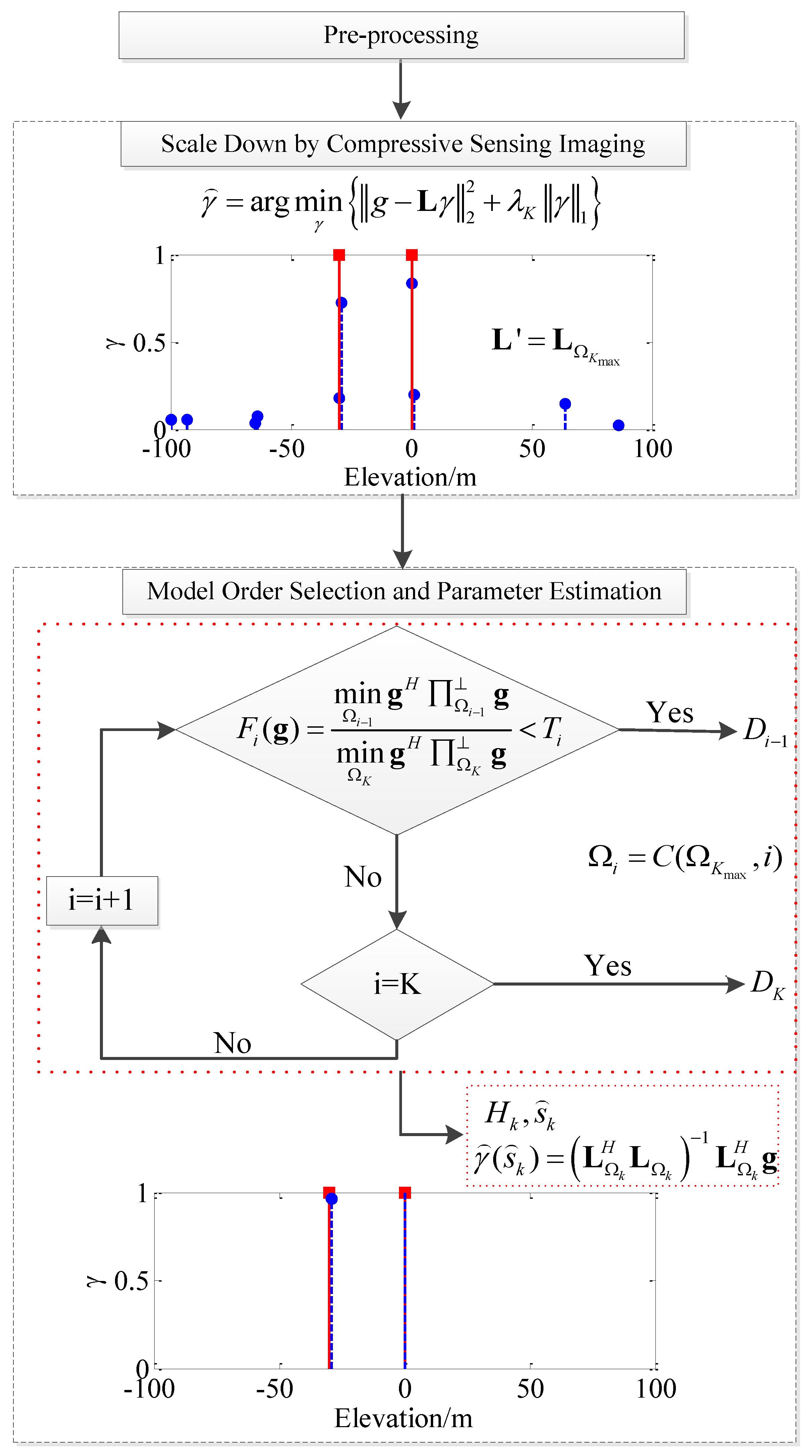
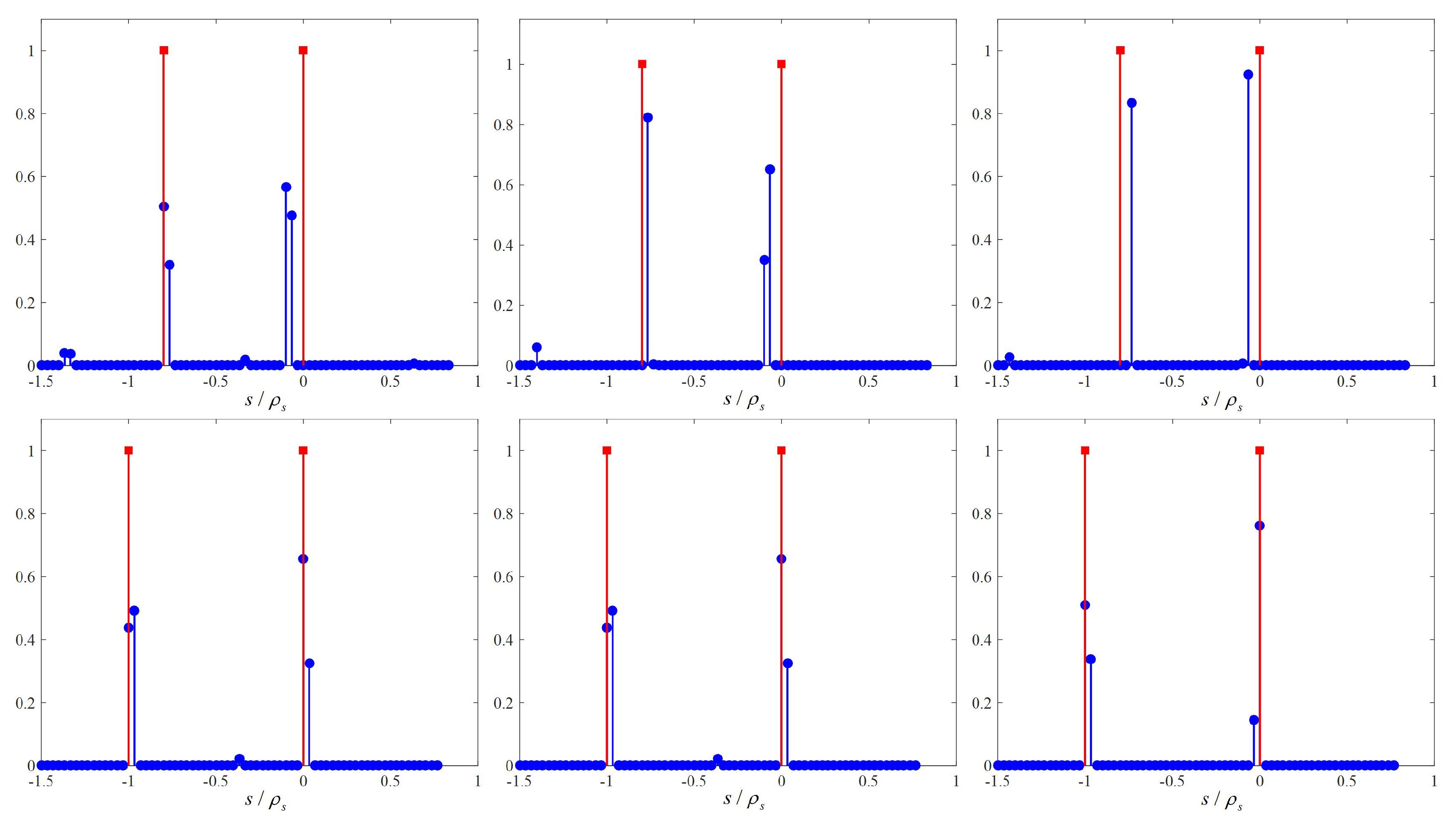
• Potential positions detection by CS imaging. In this step, the nonsignificant spurious scatterers are cleaned to offer a priori information for the possible scatterers’ locations with super-resolution so as to separate the closely located targets. Often, the number of potential positions $K_{max}$ can be set as

  $$K_{max}=max\left\{3K,{∥{\left|\gamma \right|}_{norm}>T_{zero}∥}_{L_0}\right\}$$

  (14)

  where K represents the predefined maximum number of scatterers, ${∥•∥}_{L_0}$ is the $L_0$ norm, i.e., the number of nonzero values, and ${\left|\gamma \right|}_{norm}$ means the normalized elevation profile reconstructed by CS. Here, threshold $T_{zero}$ of zero and nonzero can be set as $\frac{1}{10}$ (corresponds to a noise capacity of 20 dB) and $3K$ considers the other two possible outliers surrounding each scatterer. Exploiting the CS imaging, the problem to be solved is scaled down from M-dimension to $K_{max}$-dimension. Empirically, K can be set as 3 and $K_{max}$ is around 10.
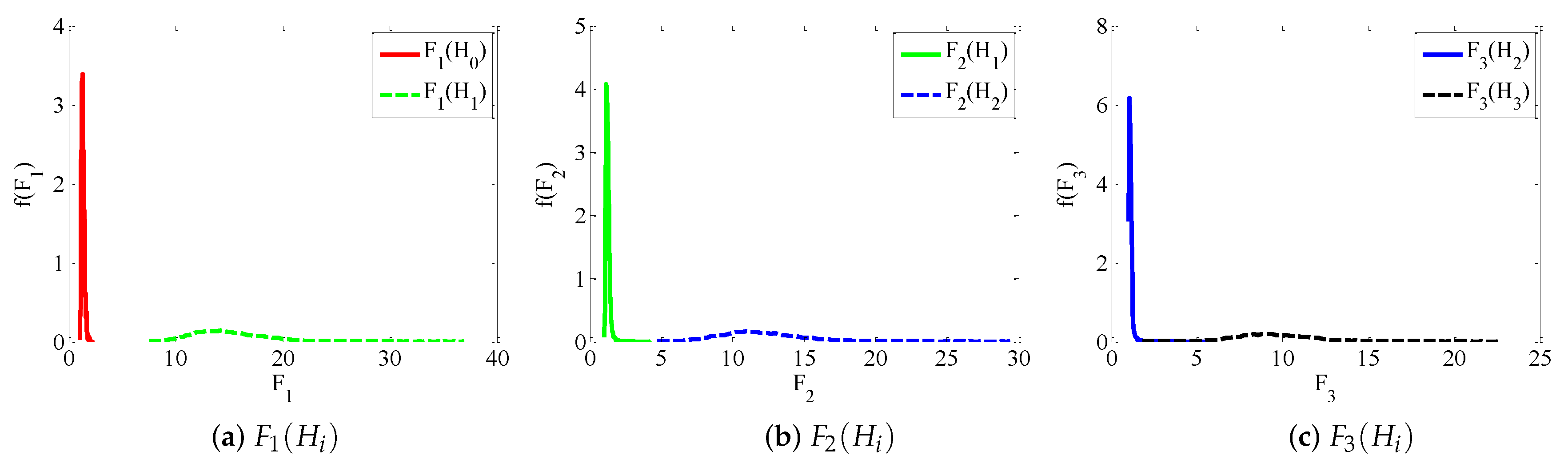
• Model order selection and parameter estimation. For each model order, $i=1,...,K$, we search for the optimal ${\Phi }_{{\Omega }_j}$ from $C_{K_{max}}^i$ possible combinations so as to minimize the numerator in Equation (10) . After obtaining the testing value of $F_i$ in each step, we can do hypothesis test sequentially, as shown in the dotted box in Figure 4. Once the model order i is selected, the elevations are the ones corresponding to the minimum numerator under the decided hypothesis and the backscattered reflectivity profile can be obtained by LS means.

Some comments on the proposed CS-GLRT method are now in order. Firstly, the computational complexity is mainly caused by the iterative steps in CS imaging, thus its computational burden is comparable to that of SL1MMER. Secondly, not all the $C_{K_{max}}^i$ possible combinations in Step 2 are valid, i.e., the combinations of scatterers located very close to each other (e.g., $D_s<\frac{1}{5}{\rho }_s$) should be dropped so as to avoid the wrong detection. Thirdly, this method suppresses the overestimation to the biggest extent as it adopts the low-to-high order detection strategy, i.e, only when the case is decided as an order higher than $H_1$ is there the possibility for the case being decided as $H_2$. Actually, there is the other strategy adopting the high-to-low order detection [19] that false alarm rate of the high order is independent of the $SNRs$ of the lower order scatterers. As a consequence, it is perfectly suitable for the small areas processing in the complex urban environment.

4. Simulated Results and Performance Assessment

We evaluated the performances of the proposed CS-GLRT based schemes by the properties of detection and accuracy, which were carried out resorting to Monte Carlo (MC) simulations. The simulated tomographic data were generated by exploiting the system parameters of a TerraSAR-X stack (see Table 1) of $N=26$ images, whose baseline distribution in the temporal/spatial domain is reported in Figure 2.

4.1. Feasibility Check

Before the implementation of the proposed algorithm, we would like to check its applicability under our systematic parameters. Firstly, the RIP is defined and tested to validate the CS imaging used here.

$$(1-{\delta }_s){∥v∥}_2^2⩽{∥\Theta v∥}_2^2⩽(1+{\delta }_s){∥v∥}_2^2,$$

(15)

where v is any vector having K nonzero coefficients at the same positions as s, and ${\delta }_s$ is a small number. ${\delta }_s$ evaluates the reconstruction sparsity of mapping matrix $\Theta$ (steering matrix $\mathbf{L}$ here). The smaller ${\delta }_s$ is, the better the sparse signal can be reconstructed in the presence of noise [15]. RIP property of two scatterers versus scatterer distance is shown in Figure 5. Figure 5a,b shows that ${\delta }_s$ increases when the scatterers come closer than ${\rho }_s$, that is to say, the closer the two scatterers are, the more sensitive the reconstruction becomes to noise. We start with two scatterers with different magnitude ratio (Figure 5a) and with constant SNR of the first scatterer, $SN{R}_1=10$ dB. It says that, in high SNR case, the system becomes less sensitive to noise with the increase of magnitude ratio. Then, RIP’s change with the alternation of phase difference is shown in Figure 5b. It says that the in-phase case ($\Delta \varphi =0$) is the most disadvantaged one, while the quadrature phase case ($\Delta \varphi =\frac{\pi }{2}$) is the most advantageous one. For these reasons, the simulations in this study adopted the most disadvantaged case, i.e., in-phase and with equal magnitude, if not specifically clarified.

Based on the fact that the number of superimposed targets within a single pixel is no more than 3 (also pointed out in [2]), K can be reasonably set as 3. Without loss of generality, we simulated up to three scatterers. To test whether there are any possibilities for the proposed CS-GLRT method of separating the overlaid scatterers within a single range-azimuth resolution cell, firstly the probability density function (PDF) of each test value $f\left(F_i\right)$ under different hypotheses $H_j$, $F_i\left(H_j\right)$, are reported in Figure 6. Figure 6a–c shows the PDFs of $F_0$, $F_1$ and $F_2$, respectively. It should be noted that all the experiments were conducted by ${10}^4$ Monte Carlo simulations with scatterers separation of ${\rho }_s$ in the hypothesis of $H_2$, and of ${\rho }_s$ and $1.5{\rho }_s$ in $H_3$, if not specifically clarified. SNR was set to 10 dB here, which is the case for persistent scatterers. The red, green, blue and black lines represent the different hypotheses of $H_0$–$H_3$, respectively. Obviously, we can see in Figure 6a that $H_0$ can be distinguished from $H_1$ by $F_1$ with no overlaps. Similarly, $H_1$ can be recognized from $H_2$ by $F_2$ with negligible overlaps. In addition, $H_2$ and $H_3$ are well separated in $F_3$ archive. It indicates that there is a great possibility that the different statistical hypotheses can be distinguished by the corresponding test values. Actually, in the experiments on simulated and real data presented in the following, setting thresholds $T_1=T_2=T_3=2$ is a good choice.

4.2. Parameter Definition

To assess the performance of the proposed CS-GLRT method, some parameters are firstly defined following the descriptions in [19]. The first one is false alarm rate $P_{fa}$ denoted as

$$P_{fa}=\frac{1}{3}[P\left(D_{1,2,3}\right|H_0)+P\left(D_{2,3}\right|H_1)+P\left(D_3\right|H_2)].$$

(16)

Then, the (correct) detection probability $P_d$ and false detection rate $P_f$ are defined as

$$\begin{array}{c}{P}_{di}=P\left(D_i\right|H_i)\hfill \\ P_{fi}={\displaystyle \sum _{j=i+1}^K}P\left(D_j\right|H_i),i=0,1,2.\hfill \end{array}$$

(17)

The last one is related to the estimation accuracy. Actually, there are three parameters, phase $\varphi$, magnitude a and elevation s. What we are really concerned about here is the accuracy of the elevation, which can be evaluated by the root mean square error (RMSE). We only consider the $P_k$ cases that the scatterer order is correctly decided, i.e., $(D_k/H_k)$, (k = 1,2,3), and the elevation RMSE is denoted as

$$RMS{E}_k=\sqrt{\frac{{\displaystyle \sum _{p=1}^{P_k}}{\displaystyle \sum _{i=1}^k}{\left({\stackrel{⌢}{s}}_{pi}-s_{pi}\right.}^2/\phantom{{\displaystyle \sum _{i=1}^k}{\left({\stackrel{⌢}{s}}_{pi}-s_{pi}\right.}^{2}k}k}{P_k}},$$

(18)

where ${\stackrel{⌢}{s}}_{pi}$ and s_pi are the estimated and true elevation positions of the ith order scatterer of the pth simulation that fulfills (D_k/H_k).

Some remarks of the performances are now in order. Often, the detection property is evaluated by the (correct) detection probability $P_d$ under a certain false alarm rate $P_{fa}$, which are given in Equations (16) and (17), respectively. $P_{fa}$ reflects the overestimation characteristic, and here we consider over-detection rate of each order of equal importance. Fixing $P_{fa}$ to get the thresholds of each step, in turn, $P_d$ can be obtained. As already explained in [20], the thresholds are insensitive to different SNRs provided that $P_{fa}$ is set.

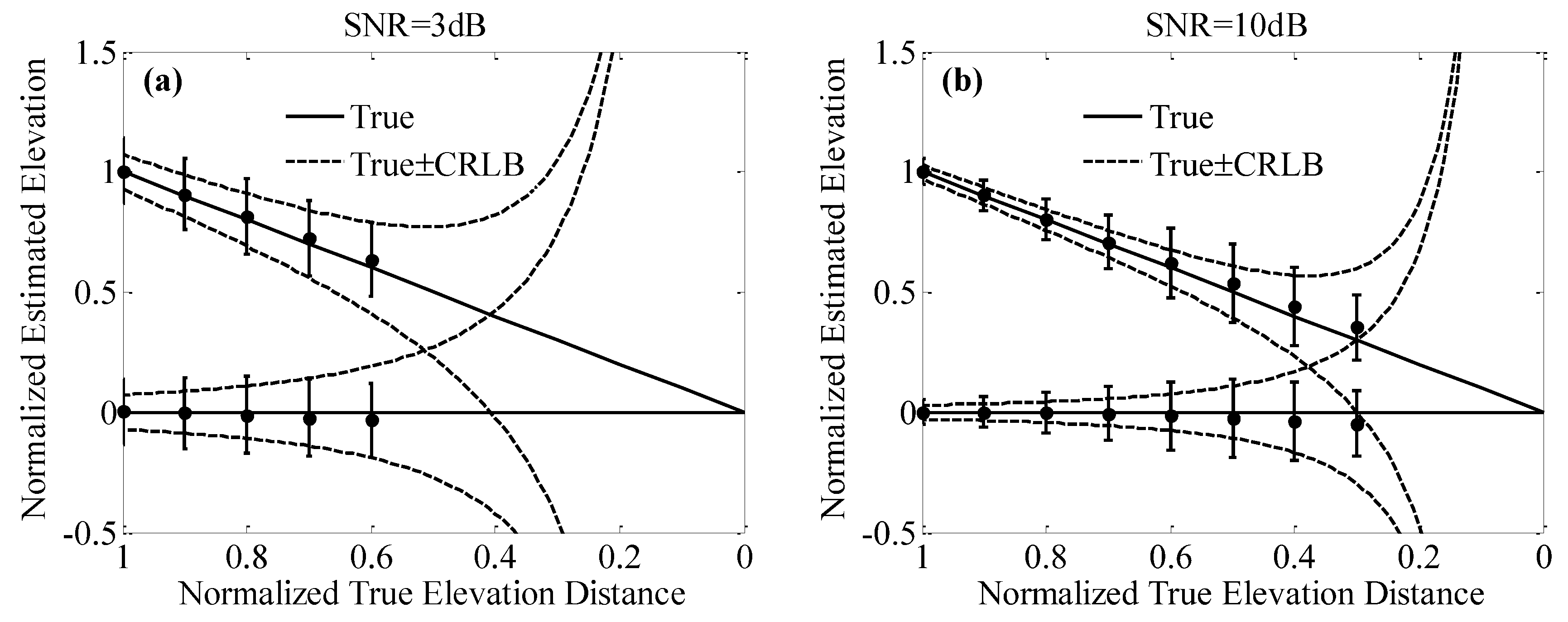
4.3. Performance Assessment

The proposed CS-GLRT method is with CFAR, or with quasi-CFAR, as the false alarm rate can be controlled by setting different thresholds, and we set $P_{fa}={10}^{-3}$ in the following experiments. The detection rate and RMSE of elevation versus $SNR$ are demonstrated in Figure 7a,b, respectively. In Figure 7a, $P_{d1}$ (red, square), $P_{d2}$ (blue, triangle) and $P_{d3}$ (green, circle) are plotted versus $SNR$ from $-15$ to 15 dB. We can see that the single, double and triple scatterers cases can be perfectly decided when SNR is big enough, e.g. 1.5, 3 and 5 dB, respectively. Then, the accuracy is demonstrated in Figure 7b and $RMS{E}_1$ (red, square), $RMS{E}_2$ (blue, triangle) and $RMS{E}_3$ (green, circle) are plotted versus $SNR$ from $-5$ to 15 dB as the detection probability is too small to show RMSE for $SNR<-5$ dB. It can be observed that, with the increase of SNR, RMSE approaches to 0, although not definitely 0 because of some estimation bias. It should be noted that $RMS{E}_3$ oscillates when the SNR is very small, e.g. SNR < 0 dB, because of the small $P_{d3}$ hardly reflecting the RMSE.

In addition, the super-resolution capability was checked by varying the distance between two scatterers from $0.4{\rho }_s$ to ${\rho }_s$. The detection probability plotted versus $SNR$ is shown in Figure 8a. It shows that, when SNR is big enough (≥8 dB), the closely located targets (up to 0.6${\rho }_s$) can be well separated with nearly $100\%P_d$. The corresponding RMSE of elevations is depicted in Figure 8b, which shows that the RMSE can be limited to 3 m ($0.1{\rho }_s$) when $SNR\ge 13$ dB for closely located scatterers (up to 0.6${\rho }_s$). Figure 8a,b jointly illustrates the super-resolution capability of CS-GLRT.

To clearly see the estimation accuracy, we compared RMSE with the accuracy obtained by CRLB. Simulations of two scatterers with different separations under $SNR=3$ dB and $SNR=10$ dB were conducted (3 dB and 10 dB are the lower and upper bound of persistent scatterers, respectively [36]). The results are shown in Figure 9a,b, respectively. It should be noted that the CRLBs shown in Figure 9 are the numerical results of Equations (A8)–(A10) and the detailed deduction of CRLBs can be referred in Appendix A.1. The solid lines show the true positions with one scatterer fixed while moving the other one. As only super-resolution cases are interested, we only show $D_s\le {\rho }_s$ here. Then, the dashed lines mark the true position ±$CRLB$ and the dots denote the mean value of the estimated elevation with the error bar being the standard deviation. Missing points indicate the detection probability below $25\%$. It should be noted that the x-axis and the y-axis are normalized to the Rayleigh resolution ${\rho }_s$. The dots approaching solid lines and error bar being nearly enveloped in the corresponding dashed lines indicate that elevation can be well estimated by the proposed CS-GLRT method.

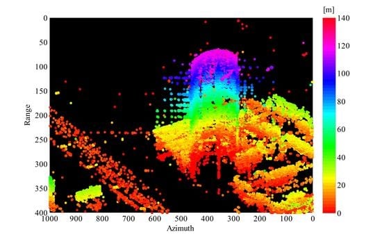
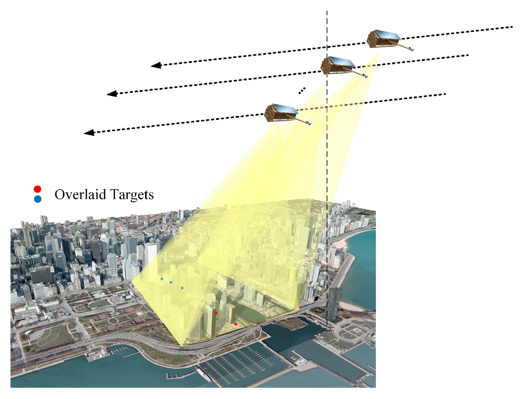
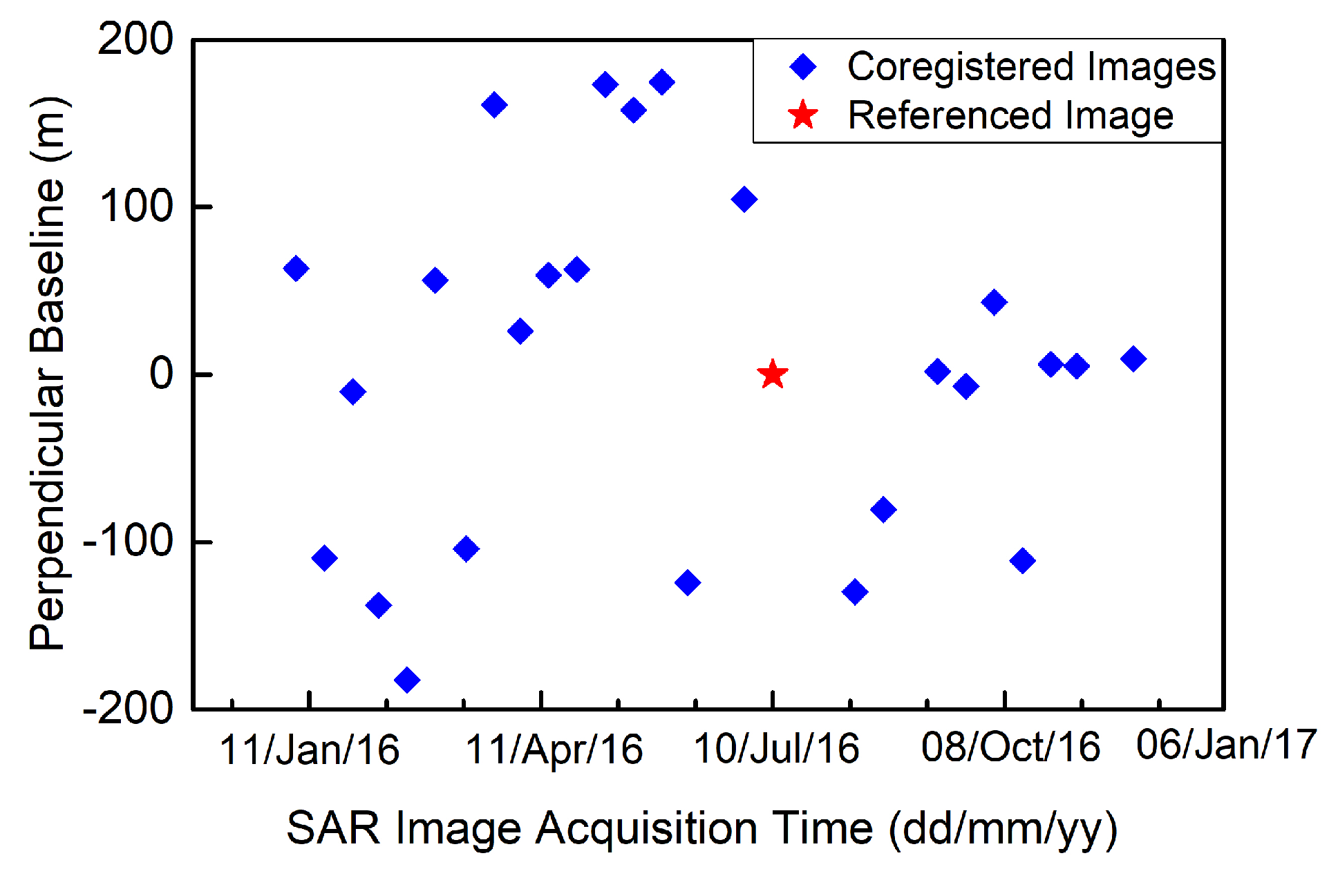
5. Results on Real Data

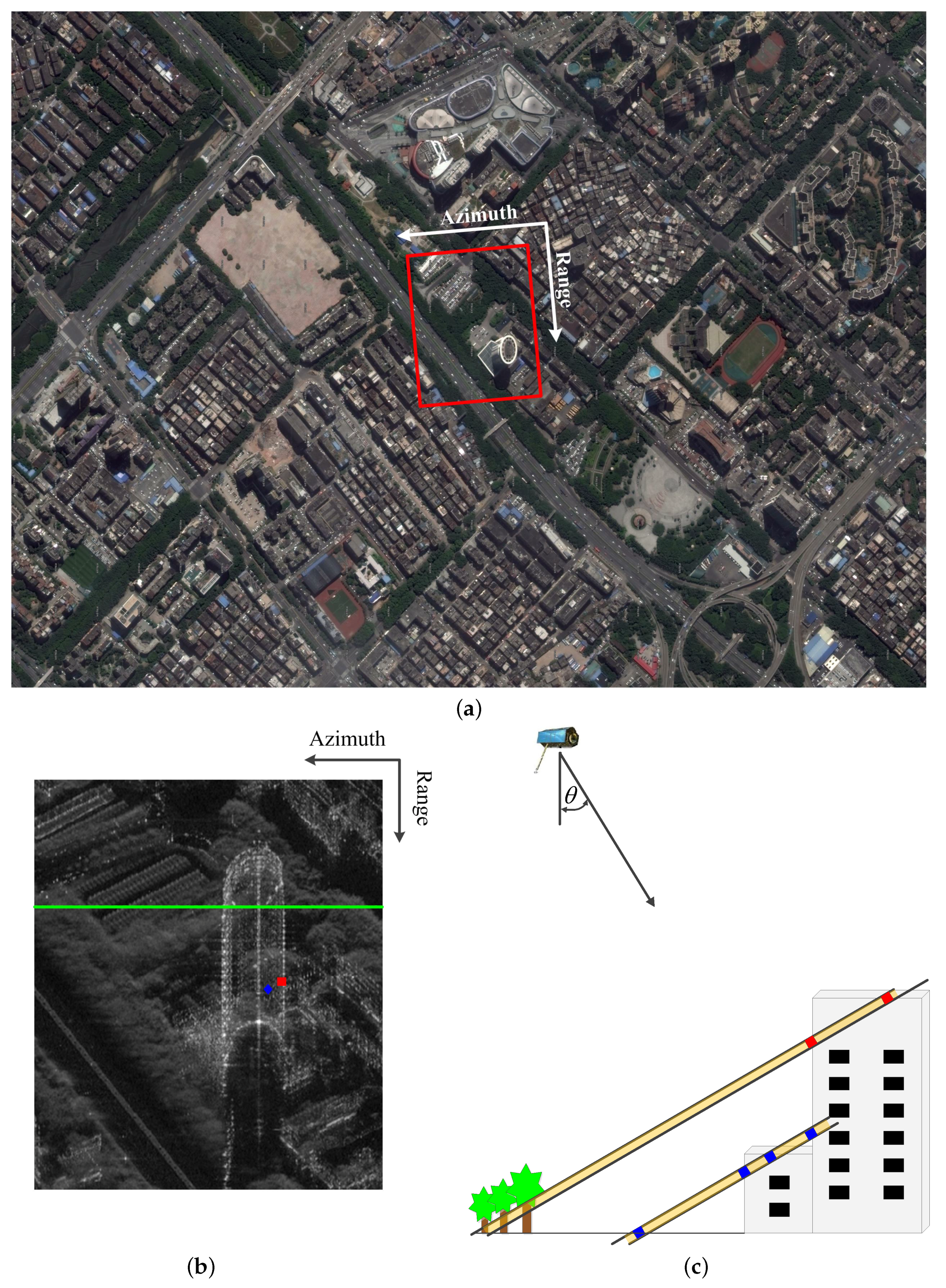
5.1. Test Site and Data Stack

Located in the south of China, Shenzhen is now one of the most developed cities in China, with a population of more than 10 million. It is highly urbanized with many high-rise buildings and dense infrastructures. A dataset of 26 scenes at 0.25 m-resolution staring spotlight TerraSAR-X images (see the system parameters in Table 1) were acquired on descending orbits during the period of the interval span from January to December 2016. To collaboratively process all the images, a referenced image acquired on 18 July 2017 was selected while the others were all coregistered to it. The spatial and temporal baseline distribution is shown in Figure 2, where the referenced one is labeled as a five-point star and the others are denoted as diamonds. As addressed above, because of the relative high burden of the CS imaging, we only tested the applicability of the proposed method on small areas, i.e., a single building.

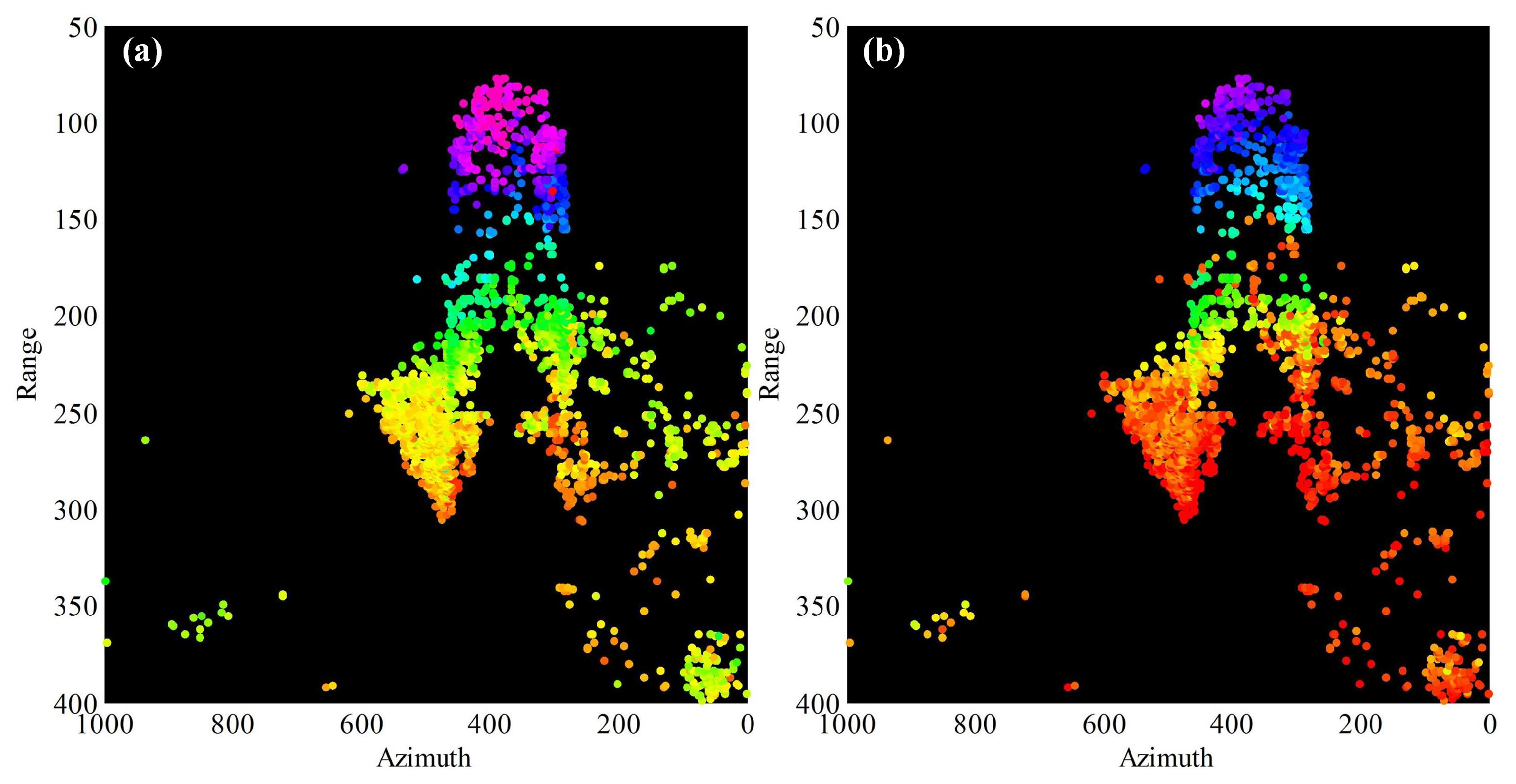
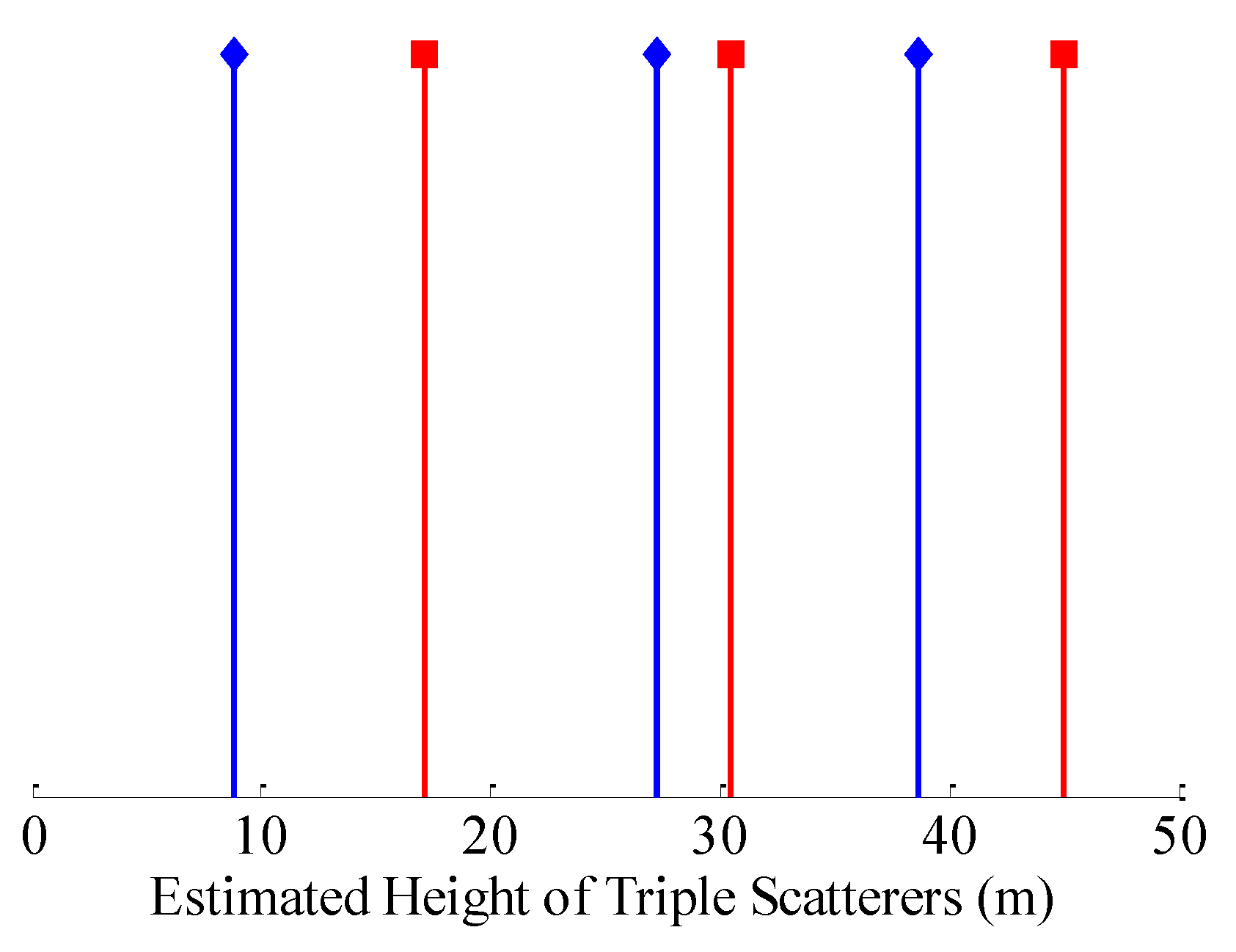
5.2. Scatterers Detection

The test area covers a high-rise building in Bao’an district (Transport Bureau Building), as shown in the optical image from Google Earth in Figure 10a (the building in the red box) and the amplitude image in Figure 10b. As shown in Figure 10a, it is a circular building with a total height of about 120 m, with a low-rise podium and some lower buildings in the neighborhood. The SAR amplitude in Figure 10b shows that the roof of the main building is probably overlaid with its own building facade and the near-range vegetation, while the roof of the podium may be superimposed with its own facade, the facade of the main building and the rough ground. Schematic drawing of possible layover cases are presented in Figure 10c, where the red squares lead to two overlaid scatterers, and the blue squares result in two, three and even four overlaid scatterers.

Before applying the proposed CS-GLRT method, the atmospheric errors should be calibrated. For the small area under study here, atmospheric error can simply be calibrated by referencing to a ground point. For atmospheric error calibration for large areas, the methods introduced in [37,38] have proven useful. The results of detected single and double scatterers are shown in Figure 11 and Figure 12, respectively, with the color bar from hot red to pink denoting heights from 0 m to 140 m. Note that the results are relative heights with respect to a near-zero point (ground point). Obviously, in Figure 11, the profile of the building is correctly detected and the estimated height range matches the true height quite well, although a few red points are found in between the building body (green), and some outliers are found along the azimuth direction. The former phenomenon was probably caused by the interference of the ground and the reflection from the building facade happens to be weak. The latter outliers were probably affected by the side lobes in azimuth, which can also be observed in the SAR intensity image (Figure 10b). To the left of the left building facade, there should only be ground targets or no targets. However, “line” targets were detected and with the same height of the pixel (same range of the line targets) on the building facade. To illustrate it, the profile of a range bin (green line in Figure 10b) is plotted, as shown in Figure 13. We adopted an up-sampling factor of 8 and only show part of the azimuth profile for a clear illustration. Under the influence of the side lobes of the strong scatterers (with the main lobe energy as large as 74 dB), many local peaks occur and are detected as targets. The appropriate restriction of side lobes is necessary and challenging in the process of SAR imaging (from L0 to L1 datatype), which is beyond the scope of this paper and will be left for the future research of SLC data preprocessing.

Figure 12 shows the height of the detected double scatterers with Figure 12a the top layer and Figure 12b the lower layer. The results agree well with the guess above that the roof of the main building is overlaid with its own facade, the main building facade is overlaid with the ground and the podium roof, respectively, and the podium roof is overlaid with its own facade and the ground, respectively. Actually, it is also possible that the triple-scatterer case happens, although with low probability (see the red square and blue diamond for their positions in SAR image in Figure 10b). The corresponding estimated heights are shown in Figure 14. We can infer that the red squares and blue diamonds are probably from the interference of the facade and roof of the lower buildings, and the tall building facade. Specifically, the number of detected single, double and triple scatterers in this experiment is 59,056, 3813 and 2, respectively.

6. Discussion

In this section, we discuss some possible comparisons of the proposed CS-GLRT with other super-resolved methods, namely SL1MMER and sup-GLRT. In addition, how to deal with ghost scatterers, which would appear to be at negative heights, is discussed.

6.1. CS-GLRT vs. SL1MMER

Theoretically, CS-GLRT has a similar computational burden, estimation accuracy and super-resolution capability as those of SL1MMER. Experimentally, using a desktop with 8 cores at 3.6 GHz and 32 GB RAM, the time consumed of ${10}^4$ MC simulations by SL1MMER and CS-GLRT is $283.1$ and $306.1$ s, respectively. Please note that parallel computing is not adopted here. The latter two performances are almost the same and are not shown here due to limited space. Here, we focus on the detection characteristics as shown in Figure 15. Scatterers can be correctly detected by SL1MMER in the $H_2$ and $H_3$ cases, yet the detection characteristic is not satisfactory in the $H_1$ case. In Figure 15b, we can see that the false detection rate of SL1MMER vibrates with $SNR$, while that of CS-GLRT remains almost stable at a very low level. Thus, SL1MMER detection is satisfactory in the high order circumstances, yet, in the lower order case, it tends to be over-decided. Usually, to alleviate computational complexity, conventional GLRT method can be carried out at first so as to distinguish the presence or absence of scatterers, thus guaranteeing a low $P_{f0}$. Nevertheless, the other false detection rate cannot be controlled, thus still leading to an unsatisfactory FAR. Therefore, CS-GLRT is a more robust method with FAR controlled.

6.2. CS-GLRT vs. Sup-GLRT

The explanation about the calculation burden is stated as follows. In [20], the maximization of the likelihood function means $C_M^i$ possible searches, and ${\displaystyle \sum _{i=0}^K}{C}_M^i$ possible searches in total, while, in our case, it scales down to $C_{K_{max}}^i$ and ${\displaystyle \sum _{i=0}^K}{C}_{K_{mapx}}^i$, respectively. M is the sampling rate along elevation with a typical value of hundreds, while $K_{max}$ is around 10 in our experiment. If we increase $K=2$ to $K=3$, the computational burden increases by approximately $\frac{M}{3}$ times for sup-GLRT, while almost remains stable for CS-GLRT. Firstly, we inspect the time consumed by sup-GLRT. Using the same desktop mentioned above, it costs 593.1 s and 112,393.6 s (31 h 13 m 13.6 s) for $K=2$ and $K=3$, respectively, if we do ${10}^4$ MC simulations and set $M=200$. As for CS-GLRT, the time consumed is 300.6 s and 306.1 s, respectively, indicating that the computational complexity remains quite stable for CS-GLRT with the change of the number of the pre-set scatterers.

The efficient version of sup-GLRT, M-sup-GLRT, can alleviate the computational burden of sup-GLRT dramatically, but its accuracy greatly depends on the correct location of the first scatterer for super-resolving. Nevertheless, the scatterers’ locations always interfere with each other and can hardly be correctly located. Thus, M-sup-GLRT is beyond the scope of this paper.

According to the analysis and experiments above,

Table 2. Performance comparison.

Method	Super-Resolution	Computational Burden	CFAR/QCFAR
CS-GLRT	high	high	Yes
SL1MMER	high	high	No
Sup-GLRT	high	very high	Yes
M-Sup-GLRT	medium	low-medium	Yes
GLRT ${}^1$	low	low	Yes

${}^1$ BF based GLRT.

compares the performances of different automatic tomographic imaging and detecting methods. We can conclude that CS-GLRT is robust and computationally acceptable for the different preset K.

6.3. Ghost Scatterers

When dealing with real data, ghost scatterers are often present, especially for large areas. There are two main sources for such ghost scatterers. The first is the limitation of estimation accuracy (CRLB), which is related to $SNR$, satellite parameters, and baseline distribution (see the details in Appendix A.1). When $SNR$ decreases, ${\sigma }_s$ deteriorates and it is possible for these points estimated with low height to be such ghost scatterers. Secondly, the miscalibattion of phase error can also contribute to such ghost scatterers. Often, isolated points with large negative heights are not likely to be genuine and can be masked in the final results. Then, point groups with moderate negative heights are likely to be genuine and can be validated further if the true structure is available. Actually, to avoid such ghost scatterers, a masking procedure is necessary prior to tomographic processing to cancel out the points with low $SNR$ and/or low correlation. Sometimes, filtering steps are useful for ghost scatterer removal. It is complicated and experience dependent, and, to our knowledge, there is no literature illustrating such a problem. Dealing with small areas, such a phenomenon is rare and easy to handle.

7. Conclusions

A multiple scatterers detection method named CS-GLRT is presented in this paper, which can super-resolve the multiple targets lying in the same azimuth-range pixel with CFAR. A two-step strategy is adopted by CS-GLRT, where the first step gets the possible candidates by super-resolution, thus scaling down the searching space in Step 2 greatly. In turn, Step 2 drops out the outliers and misdetections resorting to minimum residual of each order. Its performances can be evaluated in terms of probability of correct detection and probability of false detection. Simulations by Monte Carlo show that the proposed method can achieve a super-resolution up to $0.3{\rho }_s$ with an accuracy approaching the $CRLB$. The merits of the CS-GLRT approach are summarized as follows:

• characteristic of CFAR, controlled by the adopted thresholds;
• accurate scatterer number detection as hypothesis test adopted;
• robustness to the nonuniform baseline distribution and super-resolution capability as CS imaging adopted; and
• small calculation increase with the increase of K as a priori information of $K_{max}$ provided by CS imaging.

The practical application of the method was carried out on spotlight TerraSAR-X data over an area of Shenzhen (China), where layover effect is common under the very high resolution data. Presented results show the effectiveness of the proposed approach in detecting reliable single, double and even triple scatterers in urban areas. The very dense detection of single scatterers guarantee the effective reconstruction of manmade structures. It should be noted that only 3D reconstruction is shown here, while the application can be extended to 4D (adding velocity) and even 5D (adding velocity and thermal) with appropriate data stack.

References

1. Reigber, A.; Moreira, A. First Demonstration of Airborne SAR Tomography Using Multibaseline L-Band Data. IEEE Trans. Geosci. Remote Sens. 2000, 38, 2142–2152. [Google Scholar]
2. Budillon, A.; Johnsy, A.C.; Schirinzi, G. Urban Tomographic Imaging Using Polarimetric SAR Data. Remote Sens. 2019, 11, 132. [Google Scholar] [Green Version]
3. Zhu, X.X.; Yu, A.X.; Dong, Z.; Wu, M.Q.; Li, D.X.; Zhang, Y.S. New approach for robust and efficient detection of persistent in SAR tomography. Remote Sens. 2019, 11, 356. [Google Scholar]
4. Martin del Campo, G.D.; Shkvarko, Y.V.; Reigber, A.; Nannini, M. TomoSAR Imaging for the Study of Forested Areas: A Virtual Adaptive Beamforming Approach. Remote Sens. 2018, 10, 1822. [Google Scholar] [Green Version]
5. Li, X.W.; Liang, L.; Guo, H.D.; Huang, Y. Compressive Sensing for Multibaseline Polarimetric SAR Tomography of Forested Areas. IEEE Trans. Geosci. Remote Sens. 2016, 54, 153–166. [Google Scholar]
6. Banda, F.; Dall, J.; Tebaldini, S. Single and Multipolarimetric P-Band SAR Tomography of Subsurface Ice Structure. IEEE Trans. Geosci. Remote Sens. 2016, 54, 2832–2845. [Google Scholar]
7. Yitayew, T.G.; Ferro-Famil, L.; Eltoft, T.; Tebaldini, S. Tomographic Imaging of Fjord Ice Using a Very High Resolution Ground-Based SAR System. IEEE Trans. Geosci. Remote Sens. 2017, 55, 698–714. [Google Scholar]
8. She, Z.; Gray, D.; Bogner, R.; Homer, J. Three-dimensional SAR imaging via multiple pass processing. In Proceedings of the 1995 IEEE International Geoscience and Remote Sensing Symposium (IGARSS-95), Florance, Italy, 28 June–2 July 1995; Volume 5, pp. 2389–2391. [Google Scholar]
9. Fornaro, G.; Serafino, F.; Soldovieri, F. Three-Dimensional Focusing With Multipass SAR Data. IEEE Trans. Geosci. Remote Sens. 2003, 41, 507–517. [Google Scholar]
10. Fornaro, G.; Lombardini, F.; Serafino, F. Three-dimensional multipass SAR focusing: Experiments with long-term spaceborne data. IEEE Trans. Geosci. Remote Sens. 2005, 43, 702–714. [Google Scholar]
11. Lombardini, F.; Pardini, M.; Fornaro, G.; Serafino, F.; Verrazzani, L.; Costantini, M. Linear and adaptive spaceborne three-dimensional SAR tomography: A comparison on real data. IET Radar Sonar Navig. 2009, 3, 424–436. [Google Scholar]
12. Lombardini, F.; Pardini, M. Superresolution differential tomography: Experiments on identification of multiple scatterers in spaceborne SAR data. IEEE Trans. Geosci. Remote Sens. 2012, 50, 1117–1129. [Google Scholar]
13. Kumar, S.; Joshi, S.K.; Govil, H. Spaceborne PolSAR Tomography for Forest Height Retrieval. IEEE J. Sel. Top. Appl. Earth Obs. Remote Sens. 2017, 10, 5175–5185. [Google Scholar]
14. Sauer, S.; Ferro-Famil, L.; Reigber, A.; Pottier, E. Three-Dimensional Imaging and Scattering Mechanism Estimation Over Urban Scenes Using Dual-Baseline Polarimetric InSAR Observations at L-Band. IEEE Trans. Geosci. Remote Sens. 2011, 49, 4616–4629. [Google Scholar] [Green Version]
15. Zhu, X.X.; Bamler, R. Tomographic SAR Inversion by L1 Norm Regularization - The Compressive Sensing Approach. IEEE Trans. Geosci. Remote Sens. 2010, 48, 3839–3846. [Google Scholar]
16. Budillon, A.; Evangelista, A.; Schirinzi, G. Three-Dimensional SAR Focusing From Multipass Signals Using Compressive Sampling. IEEE Trans. Geosci. Remote Sens. 2011, 49, 488–499. [Google Scholar]
17. Budillon, A.; Ferraioli, G.; Schirinzi, G. Localization Performance of Multiple Scatterers in Compressive Sampling SAR Tomography: Results on COSMO-SkyMed Data. IEEE J. Sel. Top. Appl. Earth Obs. Remote Sens. 2014, 7, 2902–2910. [Google Scholar]
18. Maio, A.; Fornaro, G.; Pauciullo, A. Detection of Single Scatterers in Multidimensional SAR Imaging. IEEE Trans. Geosci. Remote Sens. 2009, 47, 2284–2297. [Google Scholar]
19. Pauciullo, A.; Reale, D.; Maio, A.; Fornaro, G. Detection of Double Scatterers in SAR Tomography. IEEE Trans. Geosci. Remote Sens. 2012, 50, 3567–3586. [Google Scholar]
20. Budillon, A.; Schirinzi, G. GLRT Based on Support Estimation for Multiple Scatterers Detection in SAR Tomography. IEEE J. Sel. Top. Appl. Earth Obs. Remote Sens. 2016, 9, 1086–1094. [Google Scholar]
21. Budillon, A.; Johnsy, A.C.; Schirinzi, G. A Fast Support Detector for Superresolution Localization of Multiple Scatterers in SAR Tomography. IEEE J. Sel. Top. Appl. Earth Obs. Remote Sens. 2017, 10, 2768–2779. [Google Scholar]
22. Budillon, A.; Johnsy, A.; Schirinzi, G. Extension of a Fast GLRT Algorithm to 5D SAR Tomography of Urban Areas. Remote Sens. 2017, 9, 844. [Google Scholar] [Green Version]
23. Pauciullo, A.; Reale, D.; Franze, W.; Fornaro, G. Multi-Look in GLRT-Based Detection of Single and Double Persistent Scatterers. IEEE Trans. Geosci. Remote Sens. 2018, 56, 5125–5137. [Google Scholar]
24. Danis, C.; Fornaro, G.; Pauciullo, A.; Reale, D.; Datcu, M. Super-Resolution Multi-Look Detection in SAR Tomography. Remote Sens. 2018, 10, 1894. [Google Scholar] [Green Version]
25. Zhu, X.X.; Bamler, R. Demonstration of Super-Resolution for Tomographic SAR Imaging in Urban Environment. IEEE Trans. Geosci. Remote Sens. 2012, 50, 3150–3157. [Google Scholar]
26. Zhu, X.X.; Bamler, R. Super-Resolution Power and Robustness of Compressive Sensing for Spectral Estimation With Application to Spaceborne Tomographic SAR. IEEE Trans. Geosci. Remote Sens. 2012, 50, 247–258. [Google Scholar]
27. Peng, X.; Wang, C.C.; Li, X.W.; Du, Y.N.; Fu, H.Q.; Yang, Z.F.; Xie, Q.H. Three-Dimensional Structure Inversion of Buildings with Nonparametric Iterative Adaptive Approach Using SAR Tomography. Remote Sens. 2018, 10, 1004. [Google Scholar] [Green Version]
28. Ma, P.; Lin, H.; Lan, H.; Chen, F. On the Performance of Reweighted L1 Minimization for Tomographic SAR Imaging. IEEE Geosci. Remote Sens. Lett. 2015, 12, 895–899. [Google Scholar]
29. Wang, X.; Xu, F.; Jin, Y.Q. The Iterative Reweighted Alternating Direction Method of Multipliers for Separating Structural Layovers in SAR Tomography. IEEE Geosci. Remote Sens. Lett. 2017, 14, 1883–1887. [Google Scholar]
30. Lianhuan, W.; Balz, T.; Zhang, L.; Liao, M. A Novel Fast Approach for SAR Tomography: Two-Step Iterative Shrinkage/Thresholding. IEEE Geosci. Remote Sens. Lett. 2015, 12, 1377–1381. [Google Scholar]
31. Zhu, X.X.; Ge, N.; Shahzad, M. Joint Sparsity in SAR Tomography for Urban Mapping. IEEE J. Sel. Top. Signal Proces. 2015, 9, 1498–1509. [Google Scholar] [Green Version]
32. Donoho, D.; Stodden, V.; Tsaig, Y. SparseLab. Software, Version 2.1. 2007. Available online: http://sparselab.stanford.edu (accessed on 26 May 2007).
33. Stoica, P.; Moses, R. Spectral Analysis of Signals; Prentice-Hall: Englewood Cliffs, NJ, USA, 2005. [Google Scholar]
34. Chen, S.S.; Donoho, D.L.; Saunders, M.A. Atomic decomposition by basis pursuit. SIAM Rev. 2001, 43, 129–159. [Google Scholar]
35. Zhu, X.X.; Bamler, R. Very High Resolution Spaceborne SAR Tomography in Urban Environment. IEEE Trans. Geosci. Remote Sens. 2010, 48, 4296–4308. [Google Scholar] [Green Version]
36. Adam, N.; Bamler, R.; Eineder, M.; Kampes, B. Parametric estimation and model selection based on amplitude-only data in ps-interferometry. In Proceedings of the ESA FRINGE Workshop, Frascati, Italy, 28 November–2 December 2005. [Google Scholar]
37. Ferretti, A.; Prati, C.; Rocca, F. Permanent scatterers in SAR interferometry. IEEE Trans. Geosci. Remote Sens. 2001, 39, 8–20. [Google Scholar]
38. Fornaro, G.; Pauciullo, A.; Serafino, F. Deformation monitoring over large areas with multipass differential SAR interferometry: A new approach based on the use of spatial differences. Int. J. Remote Sens. 2009, 30, 1455–1478. [Google Scholar]
39. Donoho, D.L. De-Noising by soft thresholding. IEEE Trans. Inf. Theory 1995, 41, 613–627. [Google Scholar]
40. Donoho, D.L.; Johnstone, I.M.; Kerkyacharian, G.; Picard, D. Wavelet shrinkage: Asymptopia? J. R. Stat. Soc. Ser. B 1995, 57, 301–369. [Google Scholar]
Figure 1. SAR tomography geometry of the problem under study. An array with N sensors receives signal from two or more scatterers (overlaid targets are denoted by red and blue dots). Note that distances are not in scale.
Remotesensing 11 01930 g001
Figure 2. Spatial/temporal baseline of SAR image acquisition. The red star represents the master image, while blue diamonds show the slave images.
Remotesensing 11 01930 g002
Figure 3. Diagram of the GLRT.
Remotesensing 11 01930 g003
Figure 4. Diagram of the proposed CS-GLRT. Lines in red squares are true reflectivity profiles, and lines in blue dots are the estimated reflectivity profile in each step. There are artifacts for the CS imaging, and magnitudes are underestimated. The artifacts are suppressed and magnitudes are corrected by the GLRT model order selection with negligible elevation error.
Remotesensing 11 01930 g004
Figure 5. RIP property of two scatterers versus scatterer distance (normalized to ρ s ) under different: (a) magnitude ratio with red solid, blue dashed and black dotted-dashed denoting a 1 / a 2 = 1 , 2 , 4 , respectively; and (b) phase difference with red solid, blue dashed and black dotted-dashed denoting Δ ϕ = 0 , π / 4 , π / 2 , respectively. It should be noted that S N R 1 = 10 d B and Δ ϕ = 0 are kept constant in (a), and S N R 1 = S N R 2 = 10 d B in (b). δ s refers to Equation (15).
Remotesensing 11 01930 g005
Figure 6. PDFs of F i under different hypotheses of H 0 (red), H 1 (green), H 2 (blue) and H 3 (black) with SNR=10dB and scatterers separation of ρ s for H 2 , and of ρ s and 1.5 ρ s for H 3 : (ac) the PDFs of F 1 , F 2 and F 3 , respectively.
Remotesensing 11 01930 g006
Figure 7. Performance of the proposed CS-GLRT for single (red, square), double (blue triangle) and triple (green, circle) scatterers, respectively: (a) detection probability; and (b) RMSE of the elevation.
Remotesensing 11 01930 g007
Figure 8. Super-resolution performance of the proposed CS-GLRT for the separation of 0.4 ρ s (red, square), 0.6 ρ s (blue triangle), 0.8 ρ s (green circle), and ρ s (black, diamond), respectively: (a) detection probability; and (b) RMSE of the elevations.
Remotesensing 11 01930 g008
Figure 9. Elevation accuracy of the proposed CS-GLRT compared to CRLB: (a) SNR = 3 dB; and (b) SNR = 10 dB. The y value of each dot reflects the sample mean of the estimated elevations and the corresponding error bar shows the standard deviation.
Remotesensing 11 01930 g009
Figure 10. Images of the study area: (a) optical image from Google Earth under study, with the building in the red box; (b) mean intensity map of the spotlight TerraSAR-X, with the red square and blue diamond the positions of the detected triple scatterers in SAR image, whose elevations are depicted in Figure 14; and (c) schematic drawing of possible signal contributions in a single azimuth-range pixel (size of resolution cells not to scale).
Remotesensing 11 01930 g010
Figure 11. Study result: Height of single scatterers.
Remotesensing 11 01930 g011
Figure 12. Study results for double scatterers: (a) height of the higher double scatterers; and (b) height of the lower double scatterers. Color bar is the same as that in Figure 11.
Remotesensing 11 01930 g012
Figure 13. Normalized azimuth profile corresponds to the green line in Figure 10b. Note that only part of the profile is shown for a clear illustration.
Remotesensing 11 01930 g013
Figure 14. Study results: Height of triple scatterers, corresponding the red square and blue diamond in Figure 10b.
Remotesensing 11 01930 g014
Figure 15. Detection characteristics of SL1MMER (solid) and CS-GLRT (dashed): (a) correct detection probability of single scatterer ( P d 1 , red, square), double scatterers ( P d 2 , blue, triangle), and triple scatterers ( P d 3 , green, circle); and (b) false detection probability with P f 0 (red, square), P f 1 (blue, triangle), and P f 2 ( green, circle).
Remotesensing 11 01930 g015