Spatio–Temporal Analysis of Deformation at San Emidio Geothermal Field, Nevada, USA Between 1992 and 2010


Abstract
:
1. Introduction
1.1. Interferometric Synthetic Aperture Radar
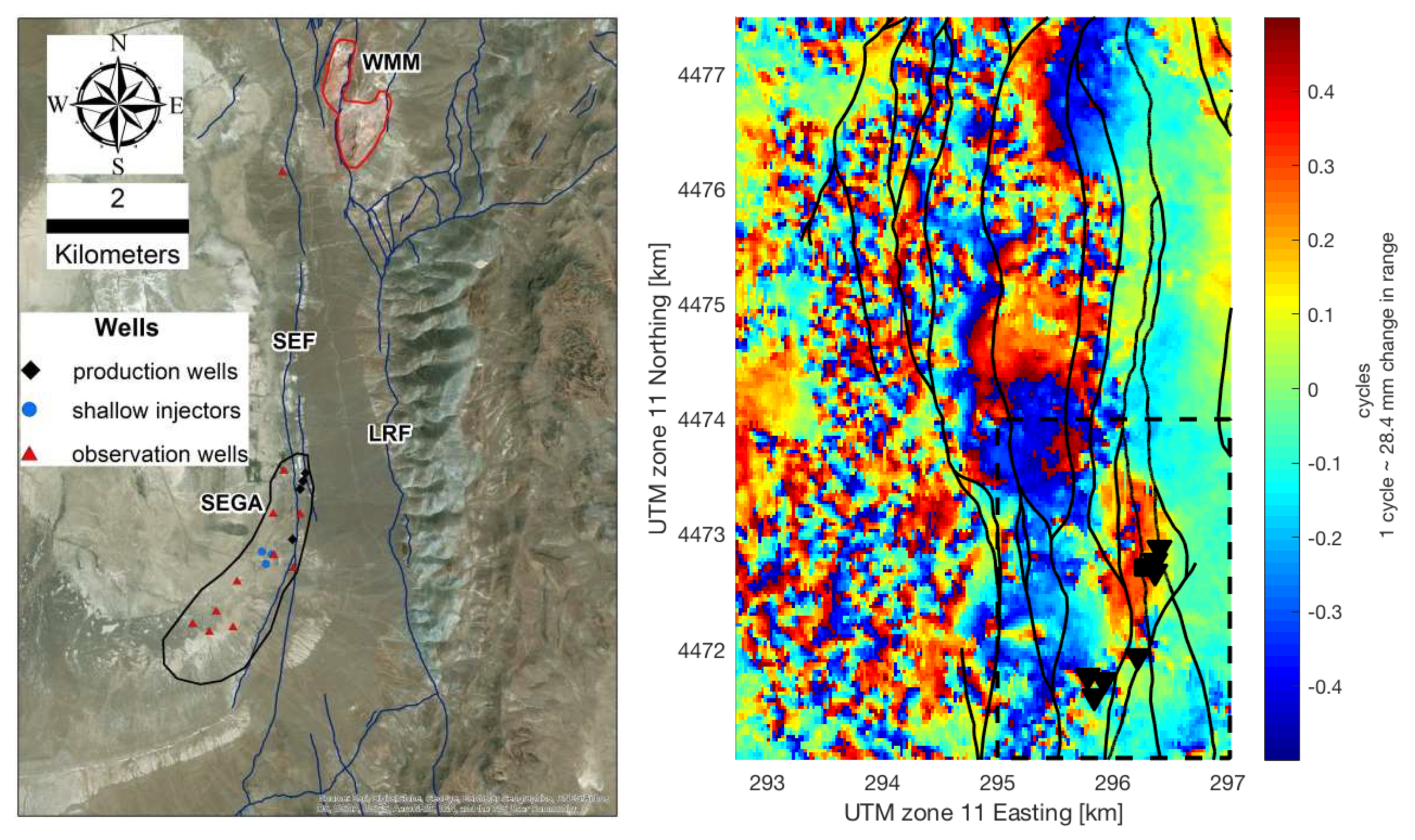
1.2. San Emidio Geothermal Field, Nevada
2. Data and Methods
2.1. Data
2.2. Methods
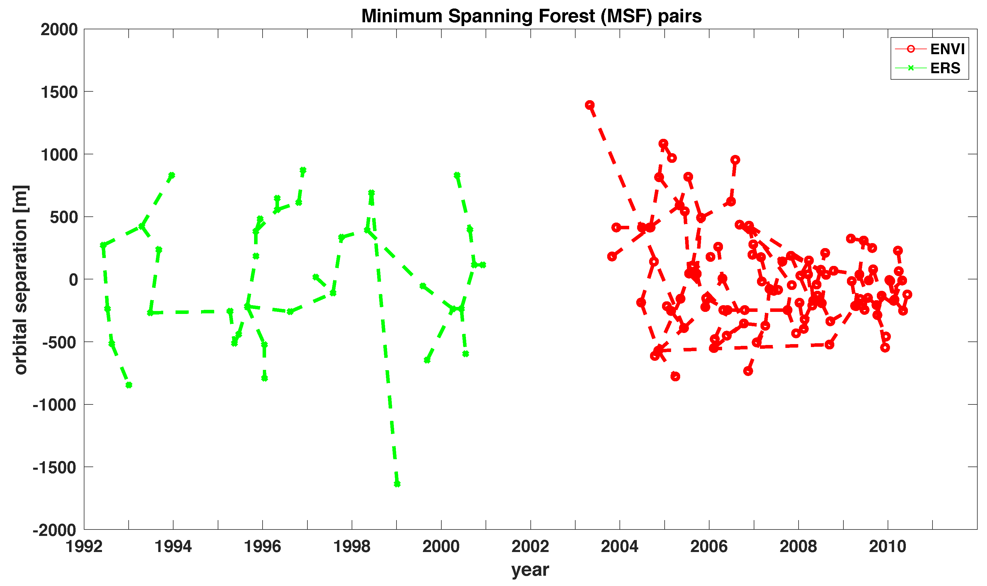
2.2.1. Selecting and Weighting Pairs
2.2.2. Deformation Modeling
2.2.3. Time-Series Analysis
3. Results
3.1. Analysis of Data Quality
3.2. Deformation Modeling
3.3. Time-Series Analysis
4. Discussion
5. Conclusions
Author Contributions
Funding
Acknowledgments
Conflicts of Interest
Abbreviations
| dof | Degrees of freedom |
| ENVI | Envisat, Environmental satellite |
| ERS | European Remote-Sensing satellite |
| InSAR | Interferometric Synthetic Aperture Radar |
| GIPhT | General inversion of phase technique |
| GMT | Generic mapping tools |
| MST | Minimum spanning tree |
| MSF | Minimum spanning forest |
| SAR | Synthetic aperture radar |
| UTM | Universal Transverse Mercator |
Appendix A. SAR and InSAR Data Sets

| Epoch (YYYY–MM–DD) | Satellite | Track | Frame |
|---|---|---|---|
| 1992–05–03 | ERS | T27 | 2799 |
| 1992–06–07 | ERS | T27 | 2799 |
| 1992–07–12 | ERS | T27 | 2799 |
| 1992–08–16 | ERS | T27 | 2799 |
| 1993–01–03 | ERS | T27 | 2799 |
| 1993–041–8 | ERS | T27 | 2799 |
| 1993–06–27 | ERS | T27 | 2799 |
| 1993–09–05 | ERS | T27 | 2799 |
| 1993–12–19 | ERS | T27 | 2799 |
| 1995–04–11 | ERS | T27 | 2799 |
| 1995–05–16 | ERS | T27 | 2799 |
| 1995–06–20 | ERS | T27 | 2799 |
| 1995–08–29 | ERS | T27 | 2799 |
| 1995–11–07 | ERS | T27 | 2799 |
| 1995–11–08 | ERS | T27 | 2799 |
| 1995–12–12 | ERS | T27 | 2799 |
| 1996–01–16 | ERS | T27 | 2799 |
| 1996–01–17 | ERS | T27 | 2799 |
| 1996–04–30 | ERS | T27 | 2799 |
| 1996–05–01 | ERS | T27 | 2799 |
| 1996–08–14 | ERS | T27 | 2799 |
| 1996–10–23 | ERS | T27 | 2799 |
| 1996–11–27 | ERS | T27 | 2799 |
| 1997–03–12 | ERS | T27 | 2799 |
| 1997–07–30 | ERS | T27 | 2799 |
| 1997–10–08 | ERS | T27 | 2799 |
| 1998–05–06 | ERS | T27 | 2799 |
| 1998–06–10 | ERS | T27 | 2799 |
| 1999–01–06 | ERS | T27 | 2799 |
| 1999–08–04 | ERS | T27 | 2799 |
| 1999–09–08 | ERS | T27 | 2799 |
| 2000–04–05 | ERS | T27 | 2799 |
| 2000–05–10 | ERS | T27 | 2799 |
| 2000–06–14 | ERS | T27 | 2799 |
| 2000–07–19 | ERS | T27 | 2799 |
| 2000–08–23 | ERS | T27 | 2799 |
| 2000–09–27 | ERS | T27 | 2799 |
| 2000–12–06 | ERS | T27 | 2799 |
| 2001–01–10 | ERS | T27 | 2799 |
| 2003–10–29 | ENVI | T120 | 801 |
| 2003–12–03 | ENVI | T120 | 801 |
| 2004–06–23 | ENVI | T27 | 2799 |
| 2004–06–30 | ENVI | T120 | 801 |
| 2004–09–01 | ENVI | T27 | 2799 |
| 2004–09–08 | ENVI | T120 | 801 |
| 2004–10–06 | ENVI | T27 | 2799 |
| 2004–10–13 | ENVI | T120 | 801 |
| 2004–11–10 | ENVI | T27 | 2799 |
| 2004–11–17 | ENVI | T120 | 801 |
| 2004–12–22 | ENVI | T120 | 801 |
| 2005–01–19 | ENVI | T27 | 2799 |
| 2005–02–23 | ENVI | T27 | 2799 |
| 2005–03–02 | ENVI | T120 | 801 |
| 2005–03–30 | ENVI | T27 | 2799 |
| 2005–05–04 | ENVI | T27 | 2799 |
| 2005–05–11 | ENVI | T120 | 801 |
| 2005–06–08 | ENVI | T27 | 2799 |
| 2005–06–15 | ENVI | T120 | 801 |
| 2005–07–13 | ENVI | T27 | 2799 |
| 2005–07–20 | ENVI | T120 | 801 |
| 2005–08–17 | ENVI | T27 | 2799 |
| 2005–09–21 | ENVI | T27 | 2799 |
| 2005–10–26 | ENVI | T27 | 2799 |
| 2005–11–30 | ENVI | T27 | 2799 |
| 2005–12–07 | ENVI | T120 | 801 |
| 2006–01–11 | ENVI | T120 | 801 |
| 2006–02–08 | ENVI | T27 | 2799 |
| 2006–02–15 | ENVI | T120 | 801 |
| 2006–03–15 | ENVI | T27 | 2799 |
| 2006–04–19 | ENVI | T27 | 2799 |
| 2006–04–26 | ENVI | T120 | 801 |
| 2006–05–24 | ENVI | T27 | 2799 |
| 2006–05–31 | ENVI | T120 | 801 |
| 2006–06–28 | ENVI | T27 | 2799 |
| 2006–08–02 | ENVI | T27 | 2799 |
| 2006–09–06 | ENVI | T27 | 2799 |
| 2006–10–11 | ENVI | T27 | 2799 |
| 2006–10–18 | ENVI | T120 | 801 |
| 2006–11–15 | ENVI | T27 | 2799 |
| 2006–11–22 | ENVI | T120 | 801 |
| 2006–12–20 | ENVI | T27 | 2799 |
| 2006–12–27 | ENVI | T120 | 801 |
| 2007–01–24 | ENVI | T27 | 2799 |
| 2007–02–28 | ENVI | T27 | 2799 |
| 2007–03–07 | ENVI | T120 | 801 |
| 2007–04–04 | ENVI | T27 | 2799 |
| 2007–05–09 | ENVI | T27 | 2799 |
| 2007–06–13 | ENVI | T27 | 2799 |
| 2007–07–18 | ENVI | T27 | 2799 |
| 2007–08–22 | ENVI | T27 | 2799 |
| 2007–10–03 | ENVI | T120 | 801 |
| 2007–10–31 | ENVI | T27 | 2799 |
| 2007–11–07 | ENVI | T120 | 801 |
| 2007–12–12 | ENVI | T120 | 801 |
| 2008–01–09 | ENVI | T27 | 2799 |
| 2008–01–16 | ENVI | T120 | 801 |
| 2008–02–13 | ENVI | T27 | 2799 |
| 2008–02–20 | ENVI | T120 | 801 |
| 2008–03–19 | ENVI | T27 | 2799 |
| 2008–03–26 | ENVI | T120 | 801 |
| 2008–04–23 | ENVI | T27 | 2799 |
| 2008–04–30 | ENVI | T120 | 801 |
| 2008–05–28 | ENVI | T27 | 2799 |
| 2008–06–04 | ENVI | T120 | 801 |
| 2008–07–02 | ENVI | T27 | 2799 |
| 2008–07–09 | ENVI | T120 | 801 |
| 2008–08–06 | ENVI | T27 | 2799 |
| 2008–08–13 | ENVI | T120 | 801 |
| 2008–09–10 | ENVI | T27 | 2799 |
| 2008–09–17 | ENVI | T120 | 801 |
| 2008–10–15 | ENVI | T27 | 2799 |
| 2009–03–04 | ENVI | T27 | 2799 |
| 2009–03–11 | ENVI | T120 | 801 |
| 2009–04–08 | ENVI | T27 | 2799 |
| 2009–04–15 | ENVI | T120 | 801 |
| 2009–05–13 | ENVI | T27 | 2799 |
| 2009–05–20 | ENVI | T120 | 801 |
| 2009–06–17 | ENVI | T27 | 2799 |
| 2009–06–24 | ENVI | T120 | 801 |
| 2009–07–22 | ENVI | T27 | 2799 |
| 2009–07–29 | ENVI | T120 | 801 |
| 2009–08–26 | ENVI | T27 | 2799 |
| 2009–09–02 | ENVI | T120 | 801 |
| 2009–09–30 | ENVI | T27 | 2799 |
| 2009–10–07 | ENVI | T120 | 801 |
| 2009–11–11 | ENVI | T120 | 801 |
| 2009–12–09 | ENVI | T27 | 2799 |
| 2009–12–16 | ENVI | T120 | 801 |
| 2010–01–13 | ENVI | T27 | 2799 |
| 2010–01–20 | ENVI | T120 | 801 |
| 2010–02–17 | ENVI | T27 | 2799 |
| 2010–02–24 | ENVI | T120 | 801 |
| 2010–03–24 | ENVI | T27 | 2799 |
| 2010–03–31 | ENVI | T120 | 801 |
| 2010–04–28 | ENVI | T27 | 2799 |
| 2010–05–05 | ENVI | T120 | 801 |
| 2010–06–09 | ENVI | T120 | 801 |
| Epoch 1 | Epoch 2 | ||
|---|---|---|---|
| 1992–06–07 | 1992–07–12 | −507.8 | 35 |
| 1992–06–07 | 1993–04–18 | 151.1 | 315 |
| 1992–07–12 | 1992–08–16 | −279.5 | 35 |
| 1992–08–16 | 1993–01–03 | −329.8 | 140 |
| 1993–04–18 | 1993–09–05 | −188.8 | 140 |
| 1993–04–18 | 1993–12–19 | 407.6 | 245 |
| 1993–06–27 | 1993–09–05 | 502.7 | 70 |
| 1993–06–27 | 1995–04–11 | 13.1 | 653 |
| 1995–04–11 | 1995–05–16 | −256.8 | 35 |
| 1995–05–16 | 1995–06–20 | 71.9 | 35 |
| 1995–06–20 | 1995–08–29 | 223.5 | 70 |
| 1995–08–29 | 1995–11–08 | 401.6 | 71 |
| 1995–08–29 | 1996–01–16 | −305.5 | 140 |
| 1995–08–29 | 1996–08–14 | −42.1 | 351 |
| 1995–11–07 | 1995–11–08 | −197.8 | 1 |
| 1995–11–07 | 1995–12–12 | 99.9 | 35 |
| 1995–11–07 | 1996–05–01 | 173.4 | 176 |
| 1996–01–16 | 1996–01–17 | −268.2 | 1 |
| 1996–04–30 | 1996–05–01 | −90.4 | 1 |
| 1996–05–01 | 1996–10–23 | 57.8 | 175 |
| 1996–08–14 | 1997–07–30 | 148.9 | 350 |
| 1996–10–23 | 1996–11–27 | 257.5 | 35 |
| 1997–03–12 | 1997–07–30 | −126.5 | 140 |
| 1997–07–30 | 1997–10–08 | 445.7 | 70 |
| 1997–10–08 | 1998–05–06 | 57.3 | 210 |
| 1998–05–06 | 1998–06–10 | 297.2 | 35 |
| 1998–05–06 | 1999–08–04 | −447 | 455 |
| 1998–06–10 | 1999–01–06 | −2326.6 | 210 |
| 1999–08–04 | 2000–04–05 | −182.5 | 245 |
| 1999–09–08 | 2000–04–05 | 410 | 210 |
| 2000–04–05 | 2000–06–14 | 0.5 | 70 |
| 2000–05–10 | 2000–08–23 | −434.2 | 105 |
| 2000–06–14 | 2000–07–19 | −359.2 | 35 |
| 2000–06–14 | 2000–09–27 | 350.5 | 105 |
| 2000–08–23 | 2000–09–27 | −282.1 | 35 |
| 2003–10–29 | 2004–09–08 | 231.9 | 315 |
| 2003–12–03 | 2004–09–08 | 315.6 | 280 |
| 2004–06–23 | 2004–10–06 | 326.7 | 105 |
| 2004–06–23 | 2004–11–10 | −385.3 | 140 |
| 2004–09–08 | 2004–11–17 | 401.8 | 70 |
| 2004–10–13 | 2005–05–11 | 456.9 | 210 |
| 2004–11–10 | 2005–03–30 | −206.1 | 140 |
| 2004–11–10 | 2008–09–10 | 48.8 | 1400 |
| 2004–11–17 | 2004–12–22 | 268.3 | 35 |
| 2004–11–17 | 2005–06–15 | −272.4 | 210 |
| 2004–12–22 | 2005–03–02 | −115.1 | 70 |
| 2005–01–19 | 2005–02–23 | −38.4 | 35 |
| 2005–05–11 | 2005–07–20 | 201.5 | 70 |
| 2005–06–15 | 2005–07–20 | −497.3 | 35 |
| 2005–07–20 | 2006–01–11 | 132.7 | 175 |
| 2005–11–30 | 2006–04–19 | 227.7 | 140 |
| 2006–02–15 | 2006–05–31 | 232.1 | 105 |
| 2006–03–15 | 2006–04–19 | −253.9 | 35 |
| 2006–04–26 | 2007–10–03 | 527.7 | 525 |
| 2006–06–28 | 2006–08–02 | 332.7 | 35 |
| 2006–11–15 | 2007–04–04 | 361.7 | 140 |
| 2006–11–22 | 2006–12–27 | −149.4 | 35 |
| 2006–11–22 | 2007–11–07 | −475.2 | 350 |
| 2006–11–22 | 2008–08–13 | −393 | 630 |
| 2006–12–20 | 2007–02–28 | −19.3 | 70 |
| 2006–12–27 | 2007–03–07 | −296.5 | 70 |
| 2007–01–24 | 2007–04–04 | 133 | 70 |
| 2007–05–09 | 2007–07–18 | −7.2 | 70 |
| 2007–06–13 | 2007–07–18 | 7.2 | 35 |
| 2007–06–13 | 2007–08–22 | 234 | 70 |
| 2007–10–03 | 2007–11–07 | 199.3 | 35 |
| 2007–10–03 | 2007–12–12 | −186.1 | 70 |
| 2008–01–09 | 2008–02–13 | −208.5 | 35 |
| 2008–01–16 | 2008–03–26 | 121.2 | 70 |
| 2008–02–13 | 2008–04–23 | 186.3 | 70 |
| 2008–02–20 | 2008–04–30 | 148.3 | 70 |
| 2008–03–19 | 2008–04–23 | −248.7 | 35 |
| 2008–03–26 | 2008–04–30 | −322.1 | 35 |
| 2008–04–30 | 2008–07–09 | −19.5 | 70 |
| 2008–05–28 | 2008–07–02 | 118 | 35 |
| 2008–05–28 | 2008–08–06 | 253.3 | 70 |
| 2008–06–04 | 2008–07–09 | −60.1 | 35 |
| 2008–07–09 | 2008–08–13 | 226.6 | 35 |
| 2008–07–09 | 2008–09–17 | −144.6 | 70 |
| 2008–09–10 | 2009–04–08 | 309.8 | 210 |
| 2008–09–17 | 2009–04–15 | 120.9 | 210 |
| 2008–10–15 | 2009–05–13 | −30.2 | 210 |
| 2009–03–04 | 2009–06–17 | −16 | 105 |
| 2009–03–11 | 2009–04–15 | −200.1 | 35 |
| 2009–04–08 | 2009–05–13 | 250.2 | 35 |
| 2009–04–15 | 2009–05–20 | 57 | 35 |
| 2009–05–13 | 2009–06–17 | 271.2 | 35 |
| 2009–05–13 | 2009–07–22 | −186.6 | 70 |
| 2009–05–20 | 2009–06–24 | −86.6 | 35 |
| 2009–06–17 | 2009–08–26 | −59.2 | 70 |
| 2009–06–24 | 2009–07–29 | 235.4 | 35 |
| 2009–07–22 | 2009–09–30 | −57.6 | 70 |
| 2009–07–29 | 2009–09–02 | 88.4 | 35 |
| 2009–09–02 | 2009–11–11 | −210.6 | 70 |
| 2009–09–30 | 2009–12–09 | −339.8 | 70 |
| 2009–09–30 | 2010–04–28 | 196.3 | 210 |
| 2009–10–07 | 2009–11–11 | 154.6 | 35 |
| 2009–10–07 | 2009–12–16 | −171.8 | 70 |
| 2009–11–11 | 2010–05–05 | −119.7 | 175 |
| 2010–01–13 | 2010–02–17 | −165.8 | 35 |
| 2010–01–20 | 2010–02–24 | −149.6 | 35 |
| 2010–02–17 | 2010–04–28 | 161.8 | 70 |
| 2010–02–24 | 2010–03–31 | 227.8 | 35 |
| 2010–02–24 | 2010–05–05 | −87.8 | 70 |
| 2010–03–24 | 2010–04–28 | −238.7 | 35 |
| 2010–05–05 | 2010–06–09 | 129.4 | 35 |


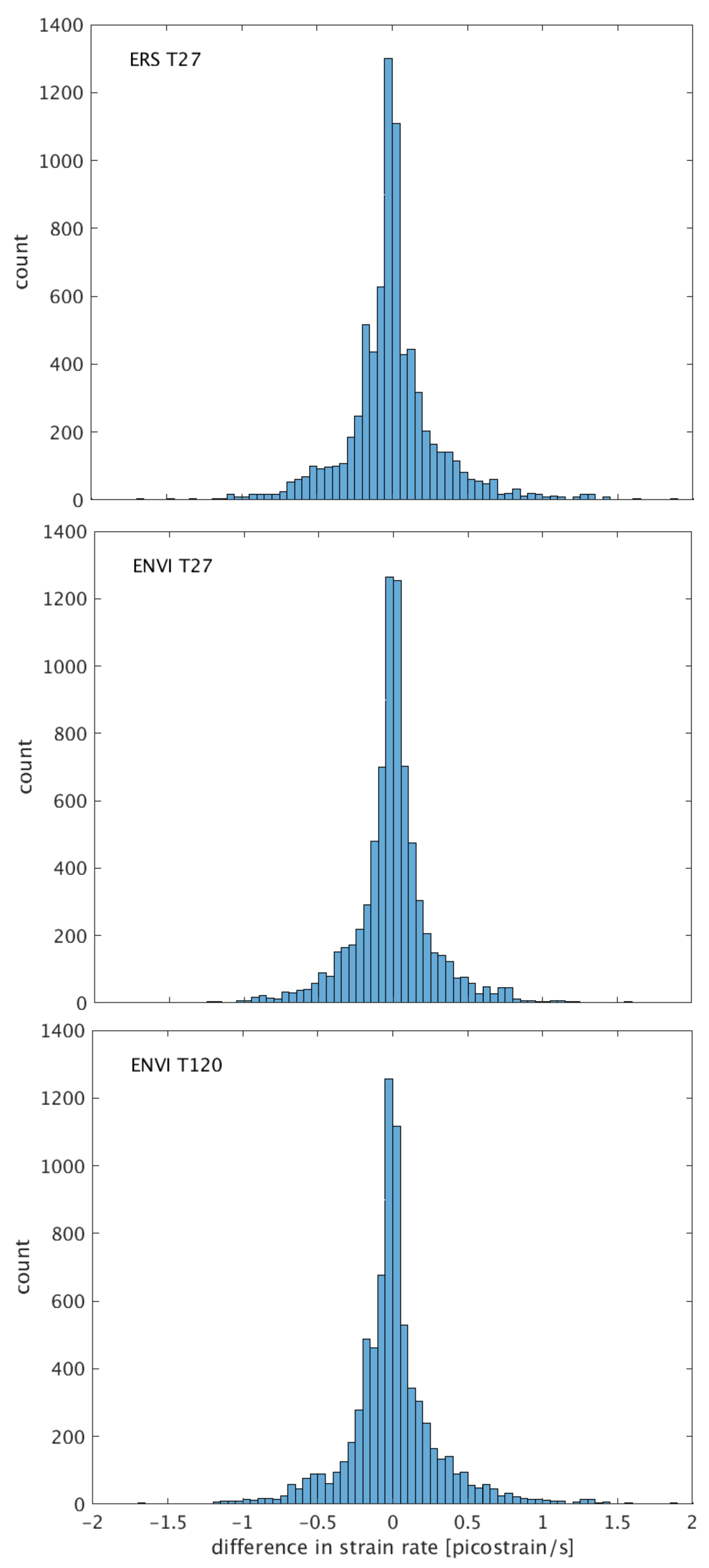
Appendix B. Strain Rate Analysis


| Data Set | SQR Sample Mean | MST Sample Mean | Differenced Mean |
|---|---|---|---|
| Data Set | and std. Deviation | and std. Deviation | and std. Deviation |
| [picostrain/s] | [picostrain/s] | [picostrain/s] | |
| ERS T27 | |||
| ENVI T27 | |||
| ENVI T120 |
Appendix C. Pumping Data


References
- Massonnet, D.; Feigl, K.L. Radar interferometry and its application to changes in the Earth’s surface. Rev. Geophys. 1998, 36, 441–500. [Google Scholar] [CrossRef]
- Moreira, A.; Prats-Iraola, P.; Younis, M.; Krieger, G.; Hajnsek, I.; Papathanassiou, K.P. A tutorial on synthetic aperture radar. IEEE Geosci. Remote Sens. Mag. 2013, 1, 6–43. [Google Scholar] [CrossRef] [Green Version]
- Massonnet, D.; Holzer, T.; Vadon, H. Land subsidence caused by the East Mesa geothermal field, California, observed using SAR interferometry. Geophys. Res. Lett. 1997, 24, 901–904. [Google Scholar] [CrossRef]
- Vasco, D.; Wicks, C., Jr.; Karasaki, K.; Marques, O. Geodetic imaging: Reservoir monitoring using satellite interferometry. Geophys. J. Int. 2002, 149, 555–571. [Google Scholar] [CrossRef]
- Liu, F.; Fu, P.; Mellors, R.J.; Plummer, M.A.; Ali, S.T.; Reinisch, E.C.; Liu, Q.; Feigl, K.L. Inferring Geothermal Reservoir Processes at the Raft River Geothermal Field, Idaho, USA, Through Modeling InSAR-Measured Surface Deformation. J. Geophys. Res. Solid Earth 2018, 123, 3645–3666. [Google Scholar] [CrossRef]
- Ali, S.; Akerley, J.; Baluyut, E.; Cardiff, M.; Davatzes, N.; Feigl, K.; Foxall, W.; Fratta, D.; Mellors, R.; Spielman, P.; et al. Time-series analysis of surface deformation at Brady Hot Springs geothermal field (Nevada) using interferometric synthetic aperture radar. Geothermics 2016, 61, 114–120. [Google Scholar] [CrossRef] [Green Version]
- Ali, S.T.; Reinisch, E.C.; Moore, J.; Plummer, M.; Warren, I.; Davatzes, N.C.; Feigl, K.L. Geodetic measurements and numerical models of transient deformation at Raft River geothermal field, Idaho, USA. Geothermics 2018, 74, 106–111. [Google Scholar] [CrossRef]
- Barbour, A.J.; Evans, E.L.; Hickman, S.H.; Eneva, M. Subsidence rates at the southern Salton Sea consistent with reservoir depletion. J. Geophys. Res. Solid Earth 2016, 121, 5308–5327. [Google Scholar] [CrossRef] [Green Version]
- Ferretti, A.; Fumagalli, A.; Novali, F.; Prati, C.; Rocca, F.; Rucci, A. A New Algorithm for Processing Interferometric Data-Stacks: SqueeSAR. IEEE Trans. Geosci. Remote Sens. 2011, 49, 3460–3470. [Google Scholar] [CrossRef]
- Xu, X.; Sandwell, D.T.; Tymofyeyeva, E.; González-Ortega, A.; Tong, X. Tectonic and anthropogenic deformation at the Cerro Prieto geothermal step-over revealed by Sentinel-1A InSAR. IEEE Trans. Geosci. Remote Sens 2017, 55, 5284–5292. [Google Scholar] [CrossRef]
- Rhodes, G.T. Structural Controls of the San Emidio Geothermal System, Northwestern Nevada; University of Nevada: Reno, NV, USA, 2011. [Google Scholar]
- Eneva, M.; Falorni, G.; Teplow, W.; Morgan, J.; Rhodes, G.; Adams, D. Surface deformation at the San Emidio geothermal field, Nevada, from satellite radar interferometry. Geotherm. Resour. Counc. Trans. 2011, 35, 1647–1653. [Google Scholar]
- Faulds, J.E. Slip and Dilation Tendency Analysis of the San Emidio Geothermal Area [data set]. Technical report, Slip and Dilation Tendency Analysis of the San Emidio Geothermal Area. University of Nevada, 2014. Available online: https://0-dx-doi-org.brum.beds.ac.uk/10.15121/1136718 (accessed on 3 August 2019).
- Warren, I.; Gasperikova, E.; Pullammanappallil, S.; Grealy, M. Mapping Geothermal Permeability Using Passive Seismic Emission Tomography Constrained by Cooperative Inversion of Active Seismic and Electromagnetic Data. In Proceedings of the 43rd Stanford Workshop on Geothermal Reservoir Engineering, Stanford, CA, USA, 12–14 February 2018. [Google Scholar]
- Snyder, J.P. Map Projections–A Working Manual; US Government Printing Office: Washington, DC, USA, 1987; Volume 1395.
- McLeod, I.H.; Cumming, I.G.; Seymour, M.S. ENVISAT ASAR data reduction: Impact on SAR interferometry. IEEE Trans. Geosci. Remote Sens. 1998, 36, 589–602. [Google Scholar] [CrossRef]
- Fletcher, K. ERS Missions: 20 Years of Observing Earth (ESA SP-1326); European Space Agency (ESA): Paris, France, 2013. [Google Scholar]
- Sandwell, D.; Mellors, R.; Tong, X.; Wei, M.; Wessel, P. Open radar interferometry software for mapping surface deformation. Eos Trans. Am. Geophys. Union 2011, 92, 234. [Google Scholar] [CrossRef]
- Sandwell, D.; Mellors, R.; Tong, X.; Wei, M.; Wessel, P. GMTSAR: An InSAR Processing System Based on Generic Mapping Tools; UC San Diego: Scripps Institution of Oceanography: La Jolla, CA, USA, 2011; Available online: http://escholarship.org/uc/item/8zq2c02m (accessed on 10 April 2019).
- Goldstein, R.; Werner, C. Radar ice motion interferometry. In Proceedings of the 3rd ERS Symposium on Space at the Service of Our Environment, Florence, Italy, 14–21 March 1997; Volume 2, pp. 969–972. [Google Scholar]
- Baran, I.; Stewart, M.P.; Kampes, B.M.; Perski, Z.; Lilly, P. A modification to the Goldstein radar interferogram filter. IEEE Trans. Geosci. Remote Sens. 2003, 41, 2114–2118. [Google Scholar] [CrossRef] [Green Version]
- Refice, A.; Bovenga, F.; Nutricato, R. MST-based stepwise connection strategies for multipass Radar data, with application to coregistration and equalization. IEEE Trans. Geosci. Remote Sens. 2006, 44, 2029–2040. [Google Scholar] [CrossRef]
- Perissin, D.; Wang, T. Repeat-Pass SAR Interferometry With Partially Coherent Targets. IEEE Trans. Geosci. Remote Sens. 2012, 50, 271–280. [Google Scholar] [CrossRef]
- Agram, P.S.; Simons, M. A noise model for InSAR time series. J. Geophys. Res. Solid Earth 2015. [Google Scholar] [CrossRef]
- Berardino, P.; Fornaro, G.; Lanari, R.; Sansosti, E. A new algorithm for surface deformation monitoring based on small baseline differential SAR interferograms. IEEE Trans. Geosci. Remote Sens. 2002, 40, 2375–2383. [Google Scholar] [CrossRef] [Green Version]
- Feigl, K.L.; Reinisch, E.C.; Ali, S.T.; Thurber, C.H.; Powell, L.; Sobol, P.; Masters, A. General Inversion of Phase Technique (GIPhT) software repository—San Emidio branch. Technical report, GitHub. 2019. Available online: https://github.com/feigl/gipht/tree/SanEmidio (accessed on 26 June 2019).
- Rodriguez, E.; Martin, J. Theory and design of interferometric synthetic aperture radars. IEE Proc. F (Radar Signal Process.) 1992, 139, 147–159. [Google Scholar] [CrossRef]
- Holzner, J. Performance of ENVISAT/ASAR Interferometric Products; ESA Special Publication: Paris, France, 2003; Volume 531. [Google Scholar]
- Reinisch, E.C.; Feigl, K.L. Envisat Tracks 27 and 120 and ERS Track 27 Interferometric Synthetic Aperture Radar Data of San Emidio Geothermal Field, Nevada, USA, 1992–2010; Technical report, DOE Geothermal Data Repository; University of Wisconsin: Madison, WI, USA, 2019; Available online: http://gdr.openei.org/submissions/1147 (accessed on 28 June 2019).
- Feigl, K.L.; Thurber, C.H. A method for modelling radar interferograms without phase unwrapping: Application to the M 5 Fawnskin, California earthquake of 1992 December 4. Geophys. J. Int. 2009, 176, 491–504. [Google Scholar] [CrossRef]
- Reinisch, E.C.; Cardiff, M.; Feigl, K.L. Graph theory for analyzing pair-wise data: Application to geophysical model parameters estimated from interferometric synthetic aperture radar data at Okmok volcano, Alaska. J. Geod. 2017, 91, 9–24. [Google Scholar] [CrossRef]
- Ali, S.; Feigl, K. A new strategy for estimating geophysical parameters from InSAR data: Application to the Krafla central volcano in Iceland. Geochem. Geophys. Geosyst. 2012, 13. [Google Scholar] [CrossRef] [Green Version]
- Malvern, L.E. Introduction to the Mechanics of a Continuous Medium; Number Monograph; Prentice-Hall, Inc.: Upper Saddle River, NJ, USA, 1969. [Google Scholar]
- Sandwell, D.T.; Price, E.J. Phase gradient approach to stacking interferograms. J. Geophys. Res. Solid Earth 1998, 103, 30183–30204. [Google Scholar] [CrossRef] [Green Version]
- Wackerly, D.; Mendenhall, W.; Scheaffer, R. Mathematical Statistics with Applications; Cengage Learning: Boston, MA, USA, 2007; 944p. [Google Scholar]
- Strang, G.; Borre, K. Linear Algebra, Geodesy, and GPS; SIAM: Philadelphia, PA, USA, 1997; 624p. [Google Scholar]
- Matlick, S. San Emidio Geothermal System; GRC Field Trip; Mesquite Group, Inc.: Hurst, TX, USA, 1995. [Google Scholar]
- Wessel, P.; Smith, W.H.; Scharroo, R.; Luis, J.; Wobbe, F. Generic Mapping Tools: Improved version released. Eos Trans. Am. Geophys. Union 2013, 94, 409–410. [Google Scholar] [CrossRef]


| Satellite | Track | ||
|---|---|---|---|
| ERS | T27 | ||
| ENVI | T27 | ||
| ENVI | T120 |
| Data Set | SQR Mean | MST Mean |
|---|---|---|
| [picostrain/s] | [picostrain/s] | |
| ERS T27 | ||
| ENVI T27 | ||
| ENVI T120 |
| Data Set | Sample Mean | Sample std. Deviation |
|---|---|---|
| [picostrain/s] | [picostrain/s] | |
| ERS T27 | 0.34 | |
| ENVI T27 | 0.28 | |
| ENVI T120 | 0.34 |
| Data Set | p-Value |
|---|---|
| ERS T27 | 0.94 |
| ENVI T27 | 0.97 |
| ENVI T120 | 0.82 |
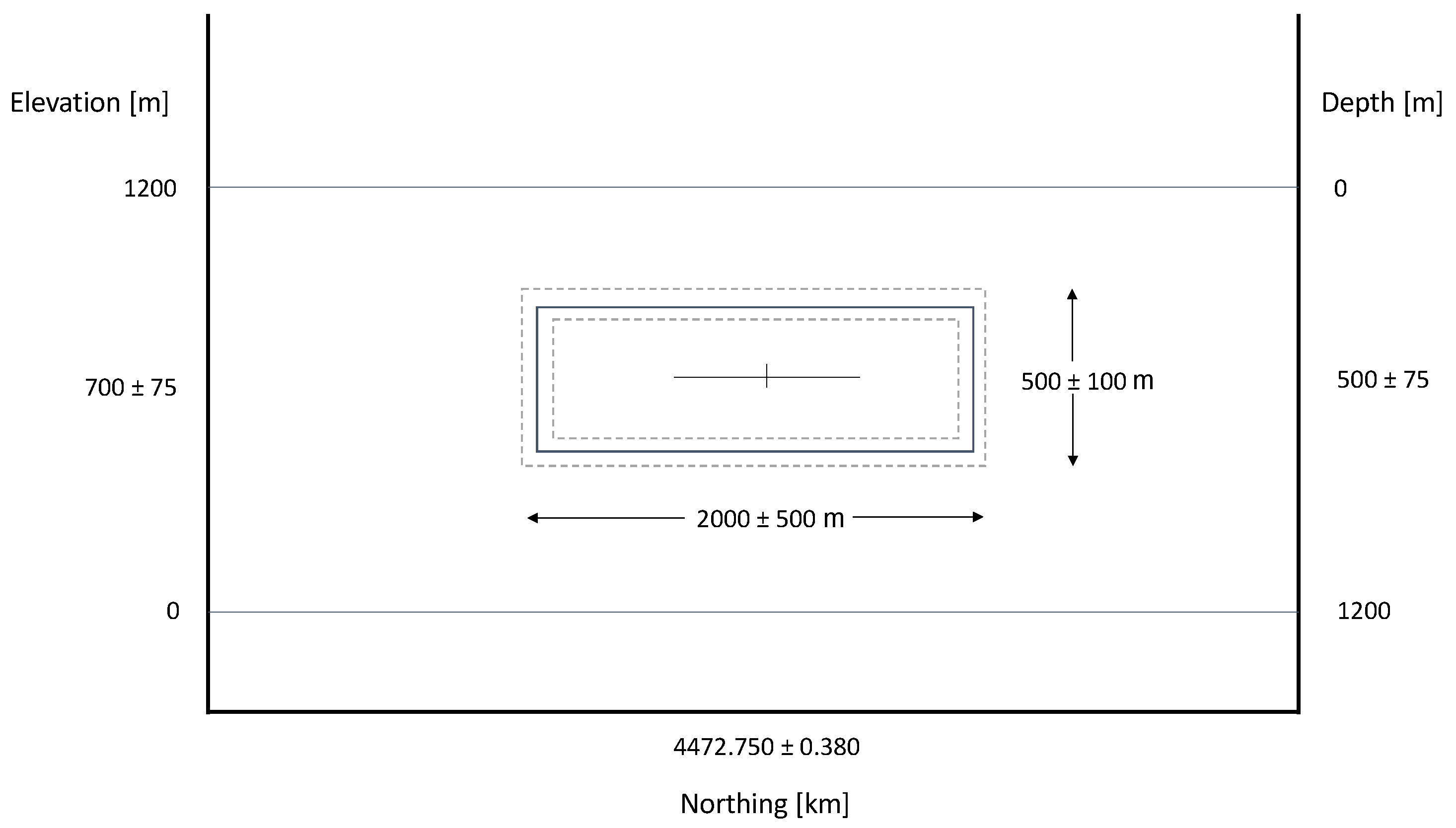
| Parameter Name | Best-Fitting Estimate | Uncertainty |
|---|---|---|
| Centroid Easting in m | 296,109 | 375 |
| Centroid Northing in m | 4,472,750 | 380 |
| Centroid Depth in m | 500 | 75 |
| Cuboid Length in m | 2000 | 500 |
| Cuboid Width in m | 200 | 50 |
| Cuboid Thickness in m | 500 | 100 |
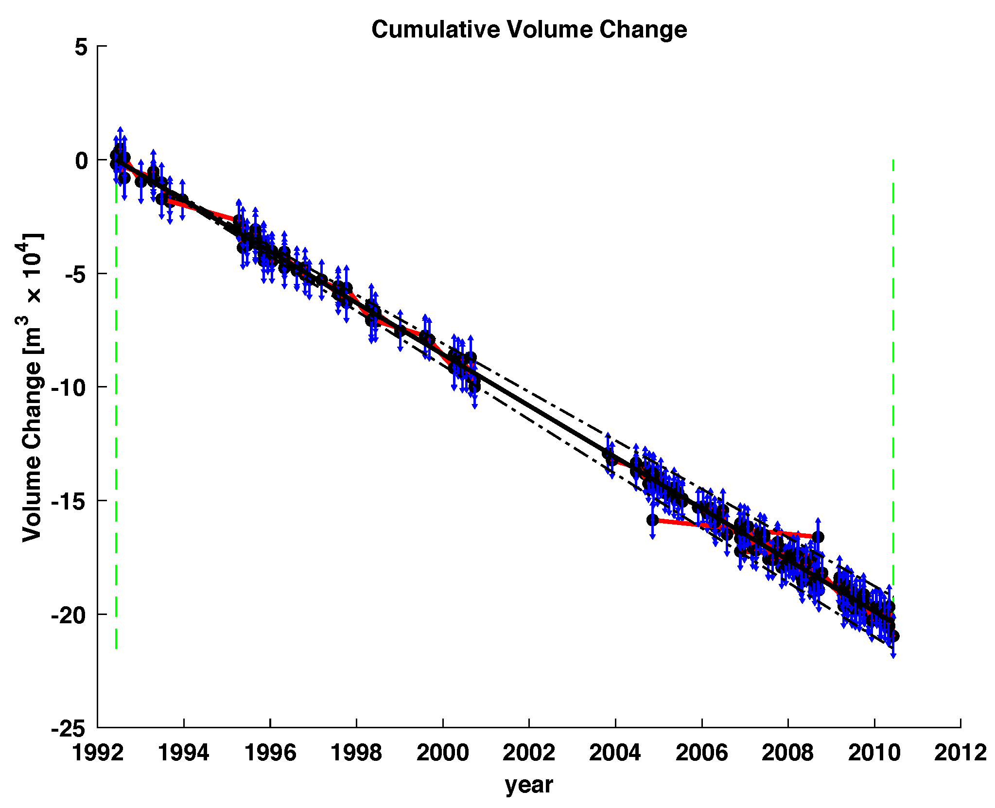
| Volume Change Rate () |
| Test Value | Critical Value | Result | ||
|---|---|---|---|---|
| 105 | 104 | −10.44 | 1.38 | fail to reject |
© 2019 by the authors. Licensee MDPI, Basel, Switzerland. This article is an open access article distributed under the terms and conditions of the Creative Commons Attribution (CC BY) license (http://creativecommons.org/licenses/by/4.0/).
Share and Cite
Reinisch, E.C.; Cardiff, M.; Akerley, J.; Warren, I.; Feigl, K.L. Spatio–Temporal Analysis of Deformation at San Emidio Geothermal Field, Nevada, USA Between 1992 and 2010. Remote Sens. 2019, 11, 1935. https://0-doi-org.brum.beds.ac.uk/10.3390/rs11161935
Reinisch EC, Cardiff M, Akerley J, Warren I, Feigl KL. Spatio–Temporal Analysis of Deformation at San Emidio Geothermal Field, Nevada, USA Between 1992 and 2010. Remote Sensing. 2019; 11(16):1935. https://0-doi-org.brum.beds.ac.uk/10.3390/rs11161935
Chicago/Turabian StyleReinisch, Elena C., Michael Cardiff, John Akerley, Ian Warren, and Kurt L. Feigl. 2019. "Spatio–Temporal Analysis of Deformation at San Emidio Geothermal Field, Nevada, USA Between 1992 and 2010" Remote Sensing 11, no. 16: 1935. https://0-doi-org.brum.beds.ac.uk/10.3390/rs11161935