Compensation of Dispersion in Sinuous Antennas for Polarimetric Ground Penetrating Radar Applications


1
Sandia National Laboratories, Albuquerque, NM 87185, USA
2
School of Electrical and Computer Engineering, Georgia Institute of Technology, Atlanta, GA 30332, USA
*
Author to whom correspondence should be addressed.
Remote Sens. 2019, 11(16), 1937; https://0-doi-org.brum.beds.ac.uk/10.3390/rs11161937
Submission received: 27 June 2019
/
Revised: 26 July 2019
/
Accepted: 12 August 2019
/
Published: 19 August 2019
(This article belongs to the Special Issue Recent Advances in Subsurface Sensing Technologies)
Abstract
:In order to improve the accuracy of subsurface target classification with ground penetrating radar (GPR) systems, it is desired to transmit and receive ultra-wide band pulses with varying combinations of polarization (a technique referred to as polarimetry). The sinuous antenna exhibits such desirable properties as ultra-wide bandwidth, polarization diversity, and low-profile form factor, making it an excellent candidate for the radiating element of such systems. However, sinuous antennas are dispersive since the active region moves with frequency along the structure, resulting in the distortion of radiated pulses. This distortion may be compensated in signal processing with accurately simulated or measured antenna phase information. However, in a practical GPR, the antenna performance may deviate from that simulated, accurate measurements may be impractical, and/or the dielectric loading of the environment may cause deviations. In such cases, it may be desirable to employ a simple dispersion model based on antenna design parameters which may be optimized in situ. This paper explores the dispersive properties of the sinuous antenna and presents a simple, adjustable, model that may be used to correct dispersed pulses. The dispersion model is successfully applied to both simulated and measured scenarios, thereby enabling the use of sinuous antennas in polarimetric GPR applications.

1. Introduction
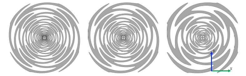
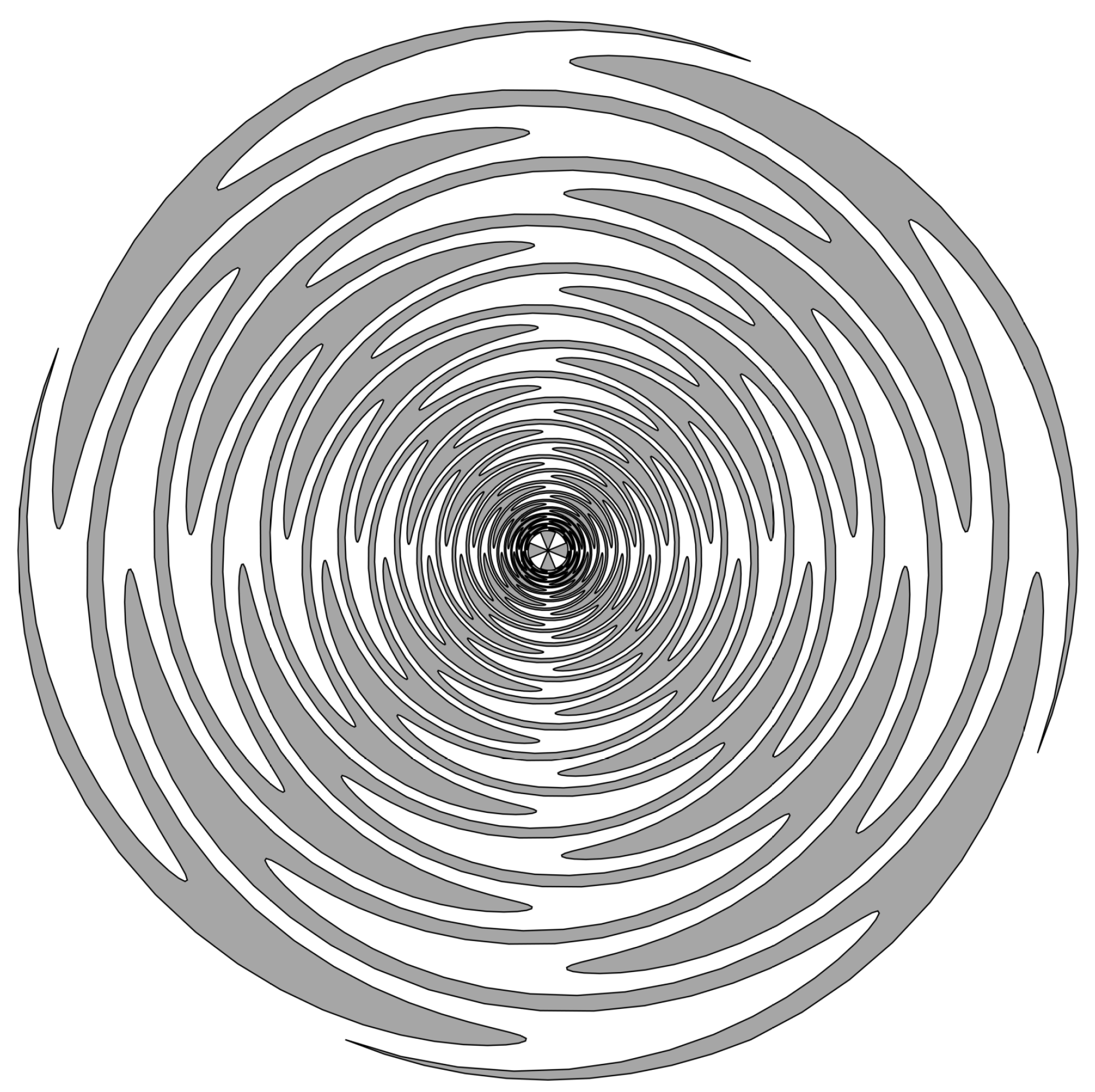
Ground penetrating radar (GPR) systems have been utilized for the detection of a diverse set of buried objects [1] largely due to their ability to sense changes in both electrical conductivity and permittivity i.e., both metal and non-metal targets [2]. The use of GPRs for the detection of buried antipersonnel landmines has been an area of extensive research [3,4]. For such applications, accurate target classification is critical, which presents challenges in GPR sensor design. Ultra-wideband (UWB) pulses are often utilized by GPR systems to improve range resolution and thus target discrimination [3]. Additionally, polarimetric radar techniques [5] have been applied to GPR to increase the accuracy of target classification [6]. These techniques require an antenna capable of producing UWB radiation at multiple polarizations. The sinuous antenna, first published in a patent by DuHamel in 1987, is an excellent candidate for such systems. The patent describes the sinuous antenna as a combination of spiral and log-periodic antenna concepts, which resulted in a design capable of producing ultra-wideband radiation with polarization diversity [7]. Other wideband antenna designs such as quad-ridge horn [8], Vivaldi [9], and resistive-vee [10] antennas provide similar capabilities. However, they require relatively large and often complex three-dimensional structures in order to produce orthogonal senses of polarization. Alternatively, the sinuous antenna (depicted in Figure 1) may be implemented as a low-profile planar structure [7]. Low profile antennas are particularly attractive for hand-held landmine detection systems that employ both GPR and metal-detector sensors [11,12].
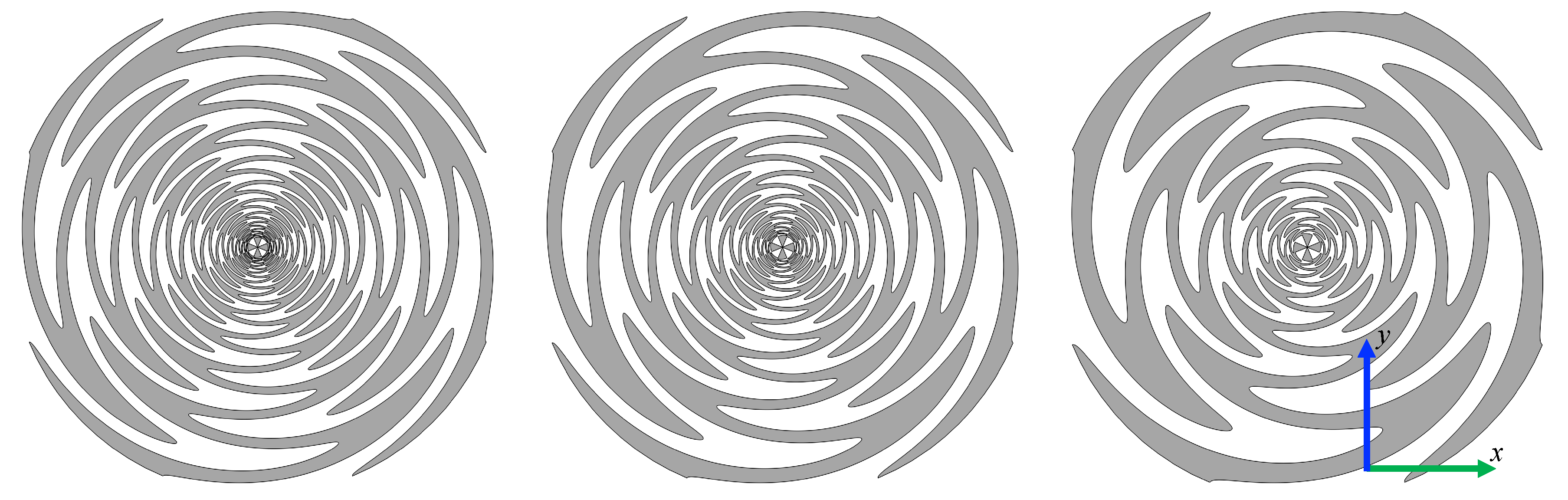
Although sinuous antennas provide the desirable properties described above, they are dispersive since the active region (see Figure 2) moves on the structure with frequency. Dispersive behavior is well documented in other log-periodic antennas such as planar spirals [13], conical spirals [14], log-periodic dipole [15,16], and planar toothed log-periodic antennas [17]. Dispersive antennas are problematic for pulsed-radar applications as the radiated pulses become distorted in the time domain, thereby reducing range resolution. Dispersed pulses may be corrected via signal processing by applying compensating phase information, which may be obtained through accurate simulation or measurement of the antenna [14]. However, for practical antennas, accurate measurement or simulation may be difficult. Furthermore, environmental effects such as thermal expansion or the dielectric loading of the soil may alter the antenna performance and thereby reduce the accuracy of previously obtained phase information. Alternatively, analytical models based on the antenna design parameters may be used to compensate for the dispersion. Such models may be desirable for GPR applications since they can be adjusted in situ to accommodate environmental effects and have low memory storage requirements. Similar analytical models have been applied successfully to GPR systems with spiral antennas [18,19]. However, for such models to remain valid when implemented for sinuous antennas, care must be taken when making antenna design decisions to avoid the excitation of unintended resonant modes, which may result in pulse distortion not correctable with simple dispersion models [20,21].
This work seeks to build an understanding of the dispersive nature of sinuous antennas and develop a model for its compensation, thereby enabling polarimetric GPR systems to obtain the benefits of sinuous antennas while utilizing them for transmitting/receiving UWB pulses with polarization diversity. Such models do not account for dispersion resulting from propagation through dispersive soil, which must be corrected by additional methods [22,23].
2. Sinuous Antenna Dispersion
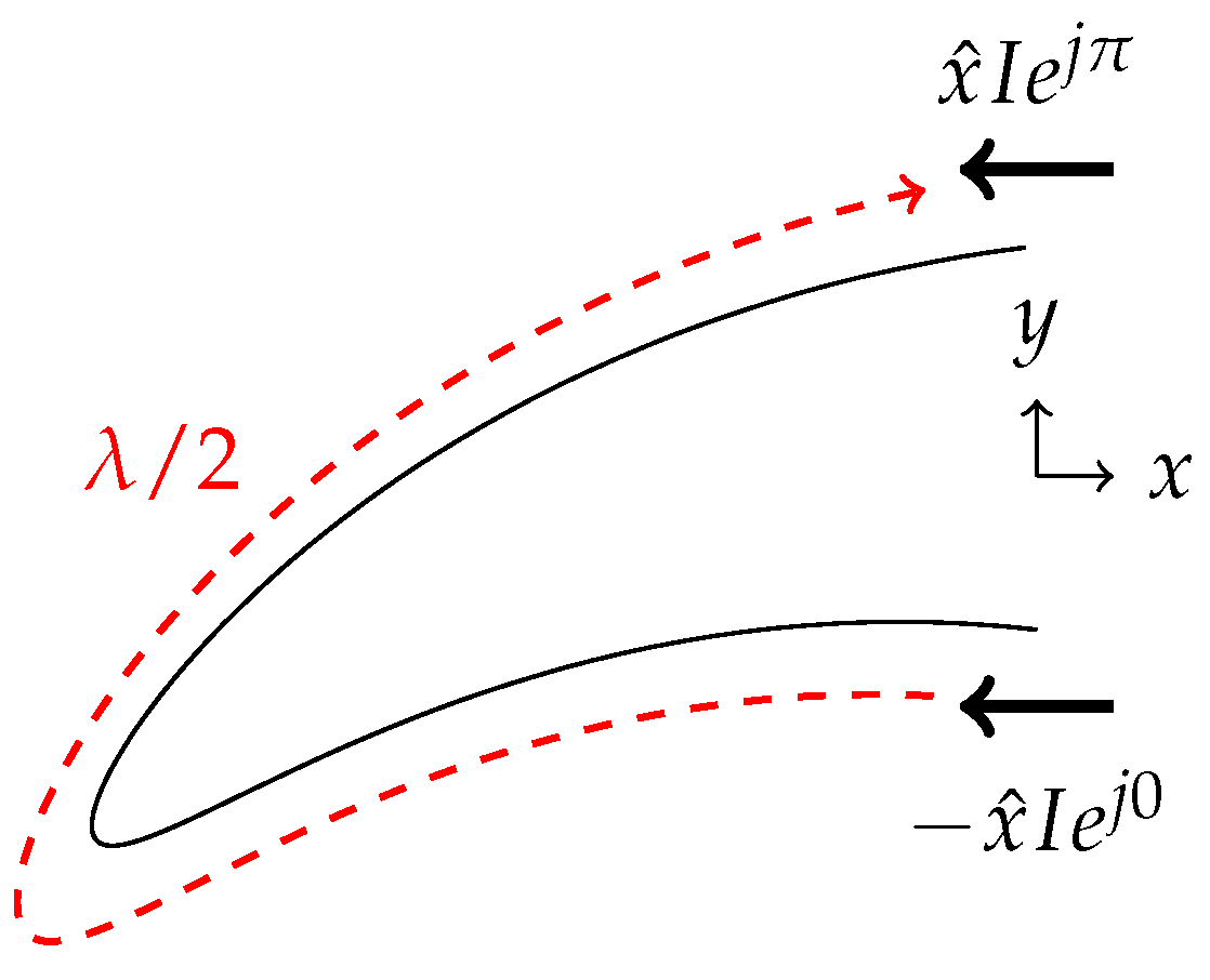
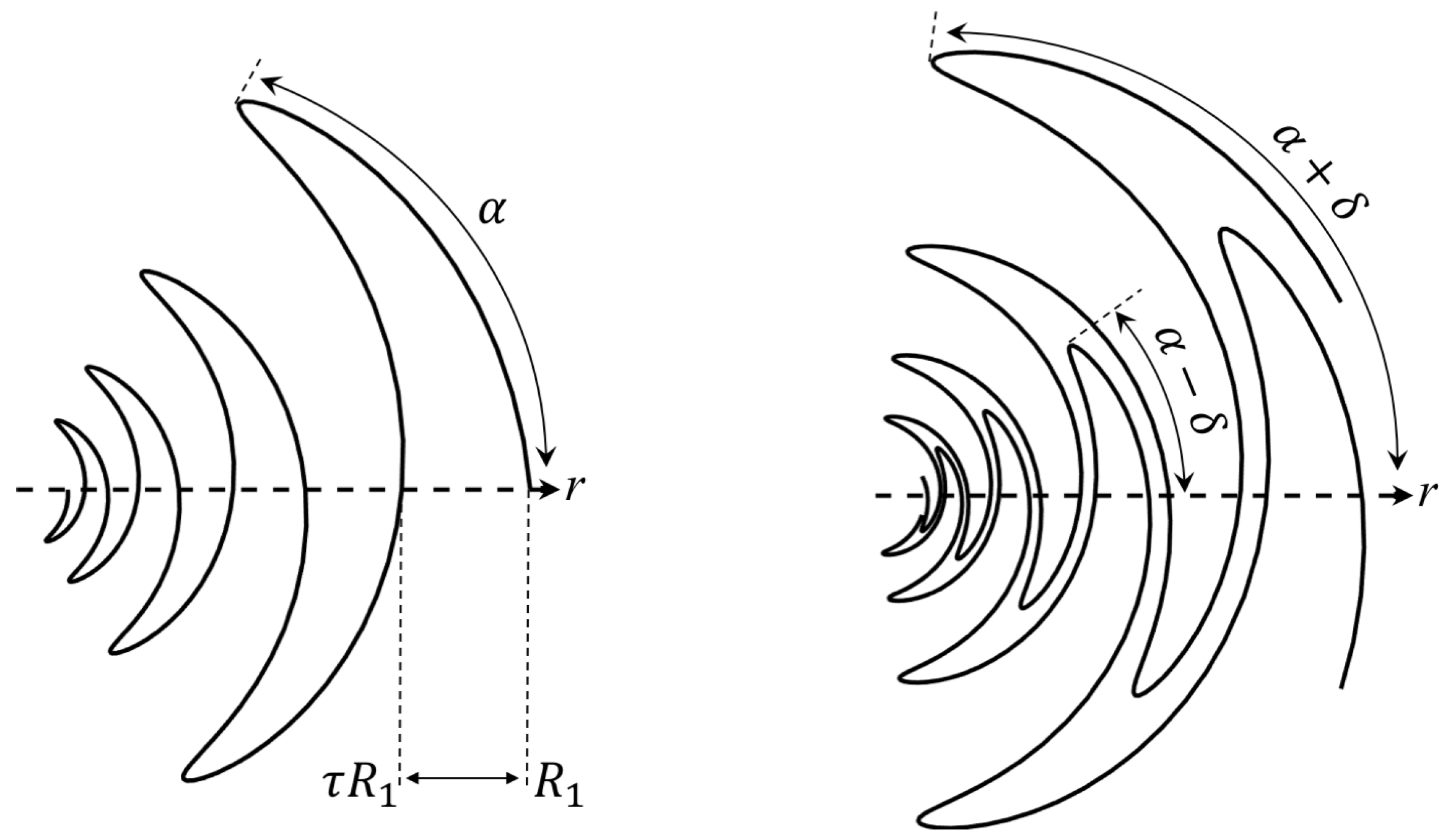
Sinuous antennas are comprised of N arms each made up of P cells where the curve of the cell is described in polar coordinates (r, ) by
where [7]. In Equation (1), controls the outer radius, the growth rate i.e., , and the angular width of the cell. The trace width of the antenna arm is controlled by rotating the sinuous curve ± the angle as illustrated in Figure 3. In this analysis, four-arm () log-periodic sinuous antennas are considered. The structures are considered log-periodic when , , and are held constant for all cells [7,24]. Additionally, is set to 22.5° in order to produce self-complementary structures. The self-complementary condition helps to ensure that the sinuous antenna’s input impedance is both real and frequency independent [25]. The antennas analyzed in this work are fed by a self-complimentary arrangement of orthogonal bow-tie elements, with radius , each feeding a set of opposing sinuous arms as illustrated in Figure 1. Furthermore, the outer truncation radius is placed at the tip of the outermost cell, i.e., , to prevent an unintended low-frequency resonance that may distort the radiation [20].
Radiation from a sinuous antenna, as described in [7], occurs at active regions that are formed when the length of a cell is approximately a multiple of . In this case, the current at the start and end of a cell is in phase due to the wrapping of the arm and travel as illustrated by Figure 2. These active regions move inward and outward on the antenna as the frequency increases and decreases respectively, resulting in a time delay between frequencies i.e., dispersion. The dispersion increases with since larger values of result in more cells i.e., longer travel times along the arms. This may encourage GPR system designers to choose small values of ; however, larger values of result in better pattern uniformity and increase operating bandwidth [7,25,26].
To investigate the dispersion, full-wave electromagnetic analysis of multiple sinuous antennas was conducted using CST Microwave Studio’s [27] time-domain solver. The sinuous antennas simulated were designed to operate from 800 MHz to 10 GHz using the following design parameters: cm, cm (bow-tie radius), = 45°, and = 22.5°. Three different values of , and subsequently P, were evaluated while maintaining all other parameters constant. Additionally, was selected as 45° in order to prevent unintended resonant modes which distort the radiation [20,21]. This will be further discussed in Section 5. The antennas (illustrated in Figure 1) were simulated in free-space (no substrate) to simplify the analysis. Both pairs of opposing sinuous arms were terminated by an ideal port set to the theoretical impedance of 267 [25]. A single pair was then driven, with the other pair remaining matched, to produce linearly-polarized radiation. The reflection coefficient and realized gain for each antenna simulated are provided in Figure 4 and Figure 5.
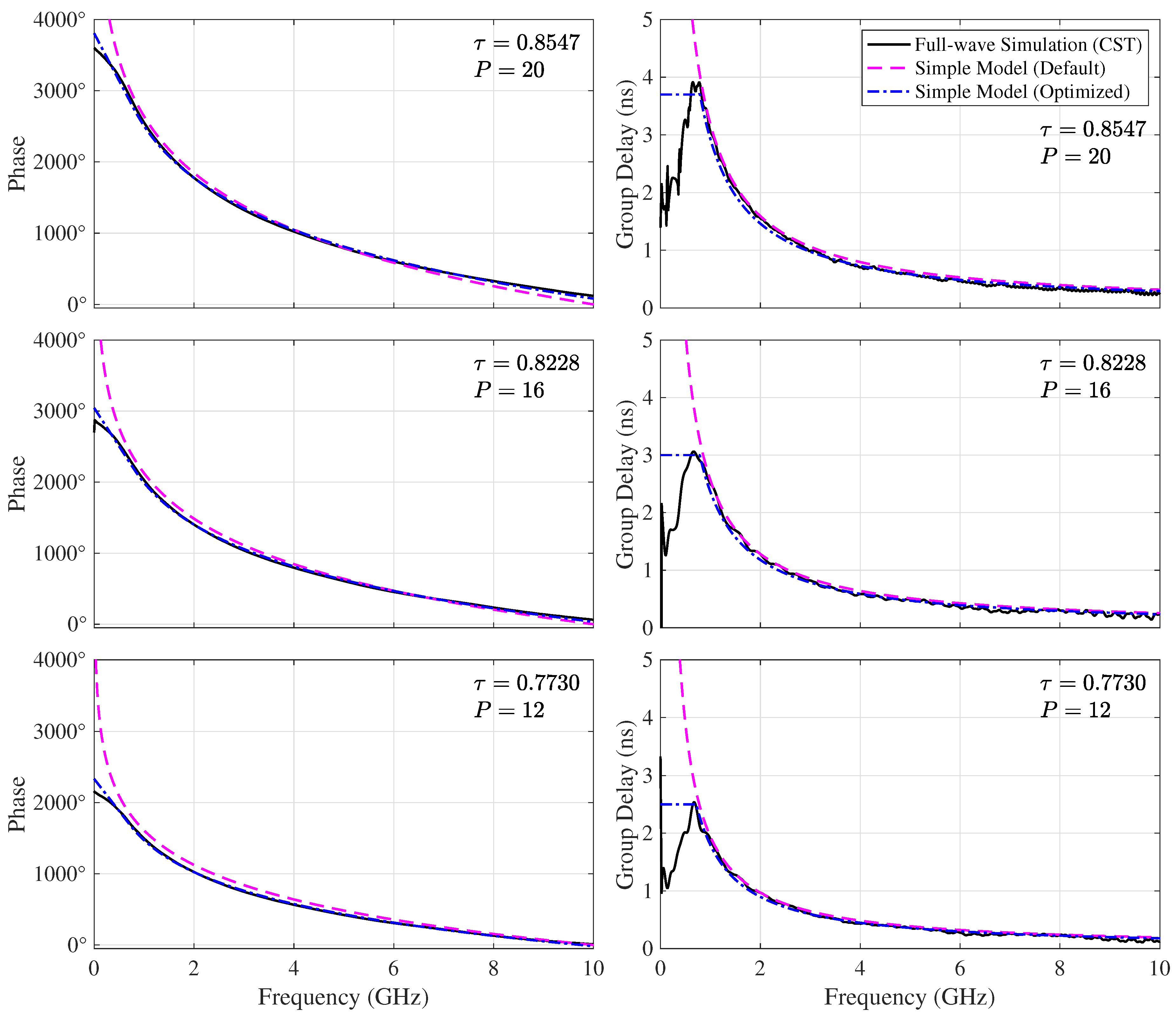
The simulated co-polarized radiated fields were probed at a boresight distance of m (far-field) and the corresponding phase was then propagated back to the antenna leaving only the phase due to dispersion
The phase is then unwrapped (starting with the 10 GHz sample) and shown in Figure 6. The corresponding group delay [17]
is also shown in Figure 6 (right column). Note that Figure 6 also displays the simple dispersion models, which will be discussed in Section 3. As expected, lower frequencies exhibit a larger delay since the corresponding active region is farther out on the antenna—where the antenna is larger. Furthermore, the results confirm the relationship between the dispersion and , i.e., increasing also increases dispersion. These effects are also evident in the time domain as will be discussed next.
The time-domain radiated pulse for a given excitation can be computed from the frequency-domain radiated fields by
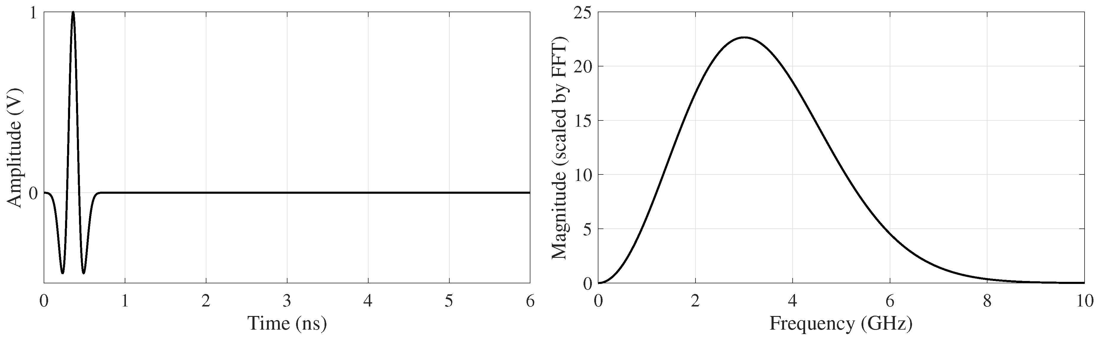
where is the frequency-domain excitation in the simulation and and are the Fourier and inverse Fourier transform, respectively. The pulse excitation used was a double-differentiated Gaussian defined as
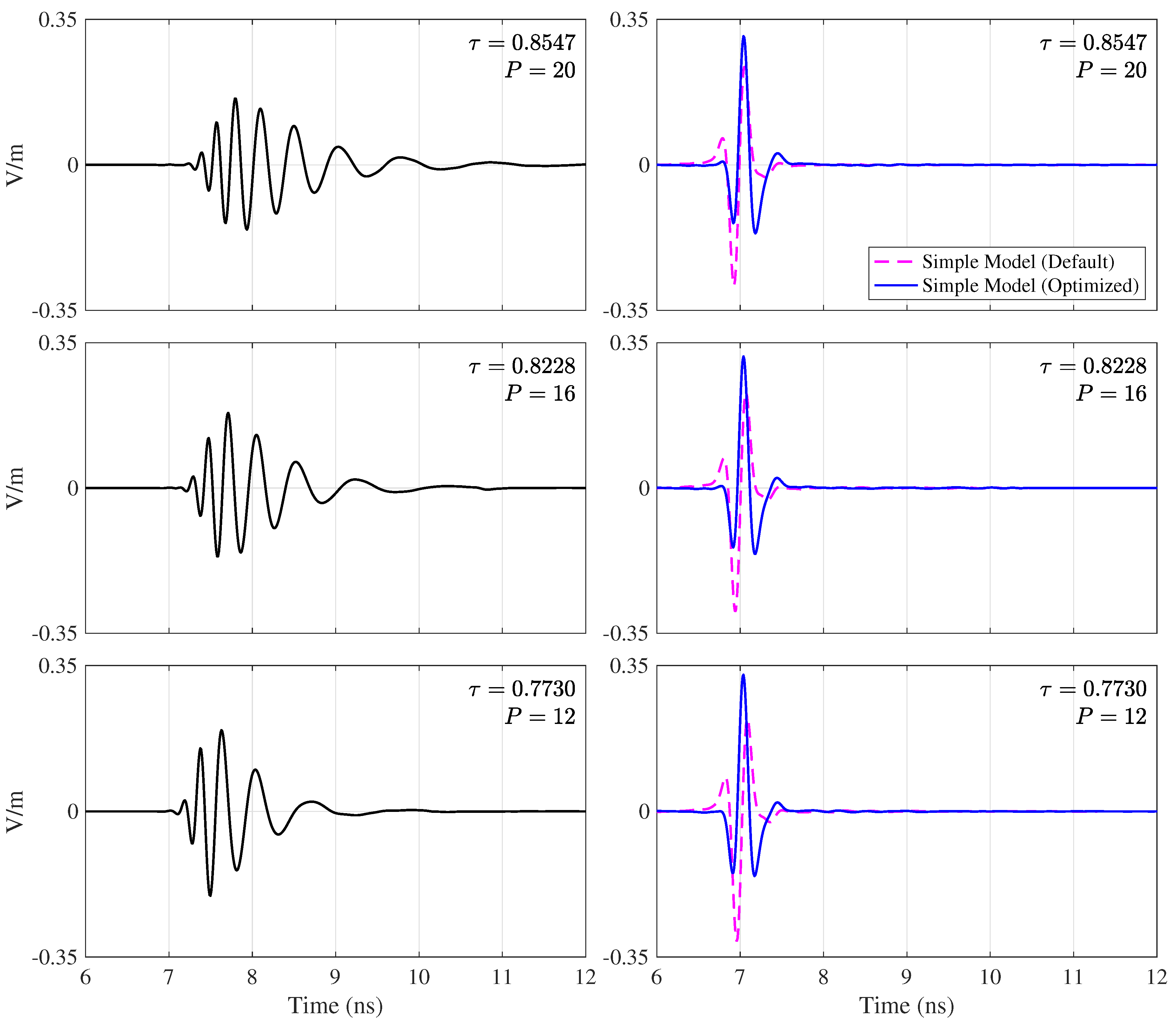
where represents an arbitrary time shift and the width of the pulse is controlled by . The double-differentiated Gaussian may be derived by multiplying the Gaussian function [28] with the second-order Hermite polynomial [29,30]. The coefficients are changed to produce a positive peak voltage at . In the presented analysis, the parameters were set to produce a 1 V peak signal at 0.36 ns with maximum spectral energy at 3 GHz (see Figure 7). The corresponding radiated pulses for the antennas simulated are shown in Figure 8. As expected from the group delay shown in Figure 6, the lower-frequency content is delayed in time from the higher-frequency content resulting in a distorted pulse with larger values of resulting in greater dispersion. It is important to note that this is only the radiated pulse; the dispersive properties will double when the antenna is used for both transmit and receive.
3. Log-Periodic Dispersion Model
Since the values of both and remain constant for each cell in the sinuous antennas analyzed, the antennas are log-periodic structures [7]. Thus, the radiated fields at frequency will repeat, since the structure repeats (scaled in size), at frequencies where n is an integer [24]. A dispersion model for log-periodic antennas has been presented in the literature [15,16,17]. As will be demonstrated, this model may also be successfully applied to log-periodic sinuous antennas.
The model represents the phase due to dispersion as
where [16]. The value controls the zero crossing of the phase model and is generally set to the highest frequency of operation (where the dispersion is defined to be zero); for this case, was used. In Figure 6, the model with the default parameters fits the stimulation results well, but with some noticeable deviation. An optimization procedure, similar to what was done in [17], may be employed to produce an improved model as shown in Figure 6. The optimization was done using MATLAB’s global optimizer [31] to find the best values for and when fitting the simulated phase , from 800 MHz to 10 GHz, starting with the initial suggested values. The default and optimized model parameters are compared in Table 1. The group delay can then be computed from the phase model using Equation (3) and is shown in Figure 6. As can be seen, the model fits the delay well with only a slight improvement obtained from the curve fit optimization. However, the model degrades at frequencies below 800 MHz where the sinuous antenna cells become electrically small and no longer radiate as intended. A similar model developed for spiral antennas implemented a constant delay below the antenna’s intended operating frequency [13]. In this work, has a constant delay imposed for frequencies below 800 MHz (see Table 1) as illustrated in Figure 6.
The optimized dispersion model was then used to correct the dispersed radiated pulse via
The radiated pulse with applied dispersion compensation is shown for each antenna in Figure 8. For comparison, Figure 8 also shows the corrected pulse computed with the default dispersion model. The applied correction causes the radiated pulse to closely match the shape of the input voltage with the optimized model giving the best result.
3.1. Off-Boresight Angles
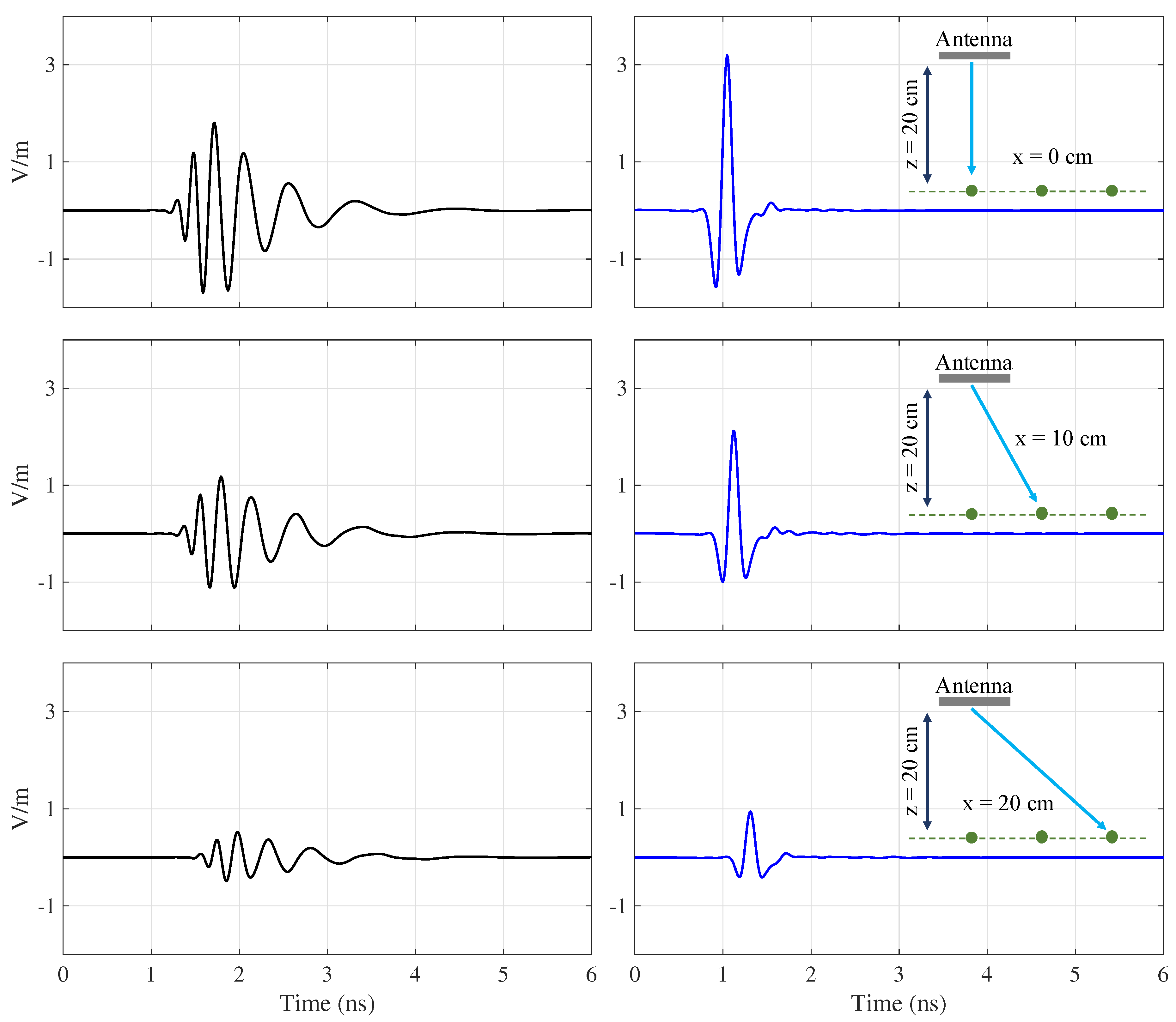
For close-in sensing applications like GPR, it is important to understand the performance of the dispersion model at off-boresight angles. In order to investigate this, simulated co-polarized radiated fields were sampled along the x-axis running parallel to the face of the 16-cell () antenna 20 cm away on boresight (). The x-axis samples are 0, 10, and 20 cm corresponding to the off-boresight angles 0°, 26°, and 45°, respectively. The dispersed radiated pulses were computed at each sample location similarly to those computed in Section 2. Both the dispersed and corrected pulses are shown in Figure 9. The parameters for the dispersion model used are from Table 1, which are optimized for m. The results show that the model can successfully correct the dispersed pulses at the off-boresight angles. Should increased accuracy be desired for imaging algorithms, separate model parameters may be stored in a look-up table corresponding to the different angles and used when the relative antenna and image pixel locations are known. The benefit of a simple model in such a case would be requiring significantly less computer memory compared to full phase datasets.
3.2. Effectiveness for Different Soil Environments
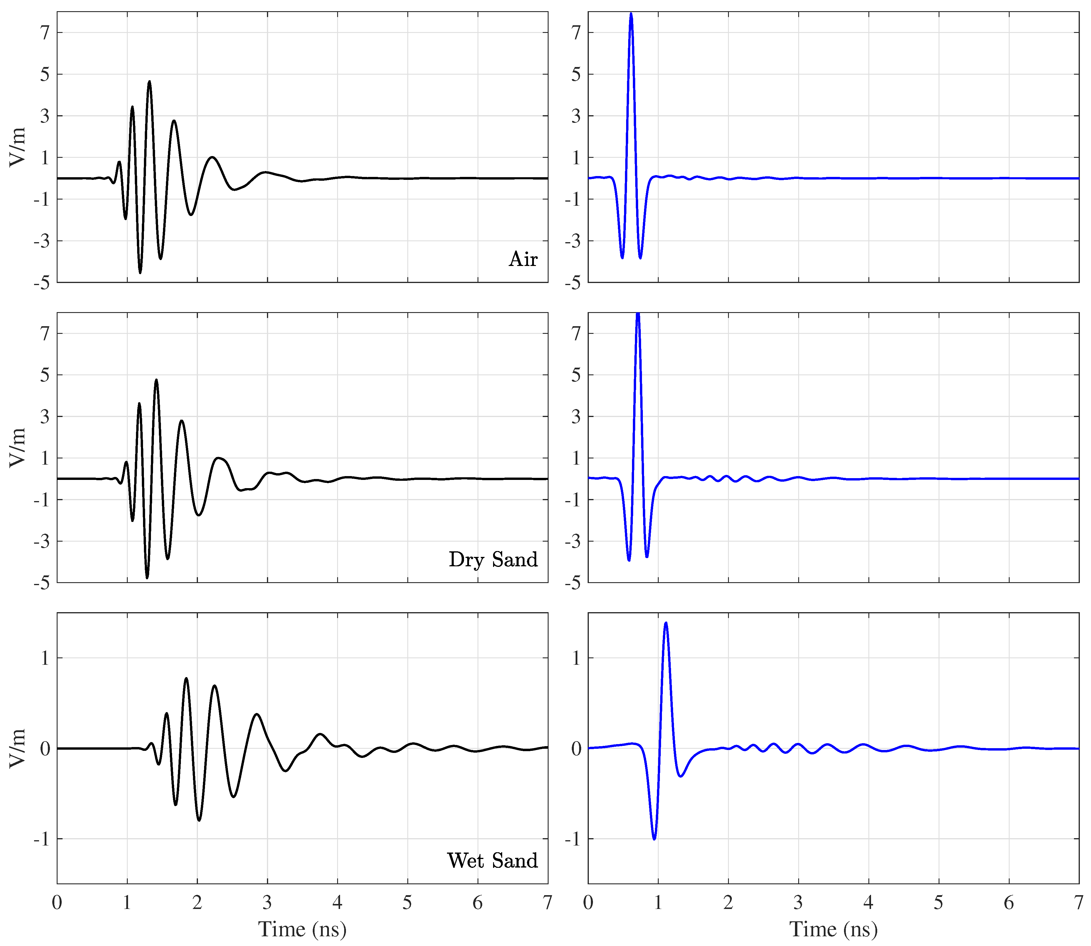
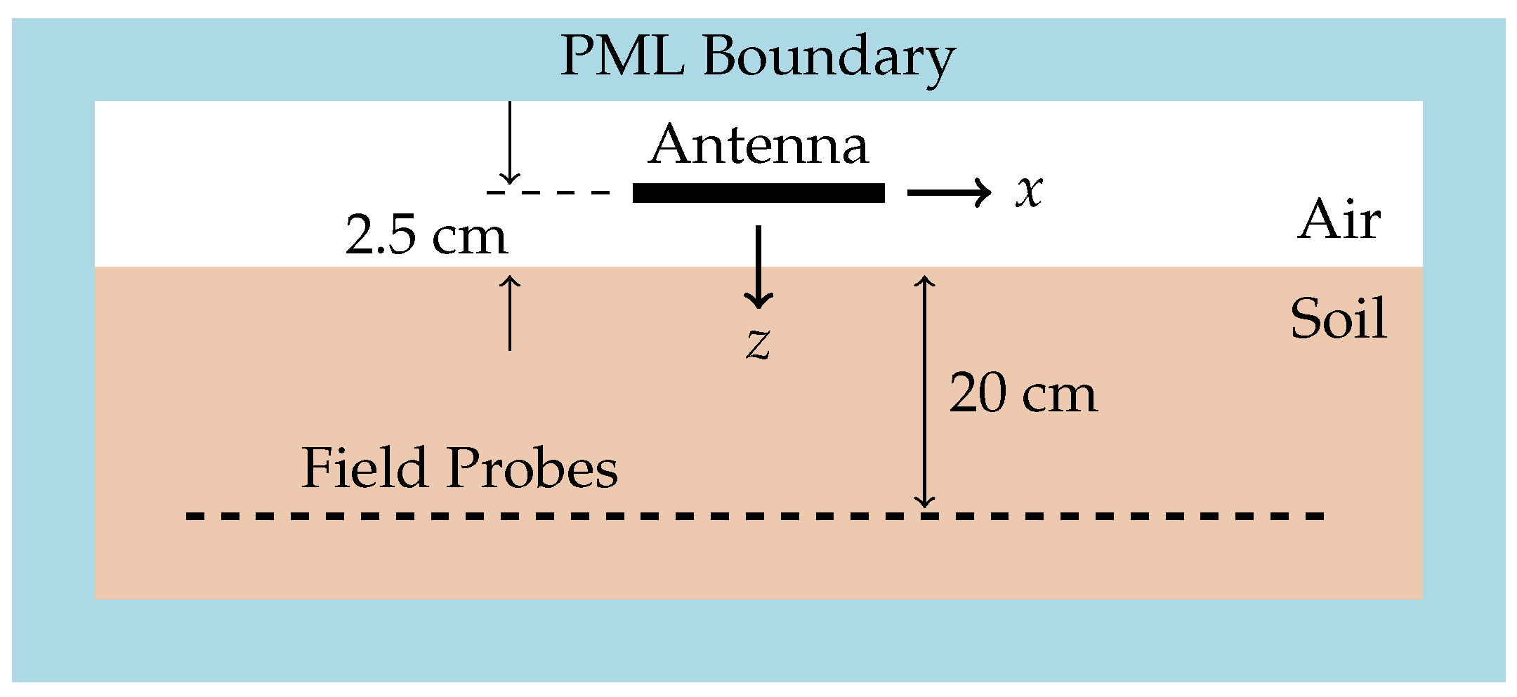
The effectiveness of the dispersion model in the presence of different soils was investigated by simulating the 16-cell antenna over both dry and wet sandy soil. The simulations were done using CST Microwave Studio’s [27] built-in dispersive models for dry and wet sandy soil. The wet sandy-soil model ( at 3 GHz) represented 18.8% moisture content and was significantly more lossy and dispersive than the dry sandy-soil model ( at 3 GHz). The antenna was placed 2.5 cm above a soil half-space and the radiated electric field was probed at a boresight depth of 5 cm below the surface. The soil was replaced with air () for comparison as well. The phase of the simulated radiated fields was propagated backward through the soil (5 cm) and free-space (2.5 cm) layers to the antenna, using the appropriate propagation constant per frequency, leaving approximately only the phase due to dispersion. The dispersion model was then fit to this phase—similar to what was done in Section 2. The optimized dispersion model parameters show little difference between materials: equal to 14.80, 14.80, 14.74 for the air, dry sand and wet sand, respectively. This indicated the presence of the soil had a negligible effect on the antenna’s dispersion.
The results, shown in Figure 10, indicate that the dispersion model is effective at removing the dispersion from the antenna; however, it does not remove dispersion due to propagation through the soil. The effects of the slight soil dispersion in the dry sand case and the moderate soil dispersion in the wet sand case are evident in the graphs. Such effects of the soil must be compensated by additional methods [22,23]. Additionally, both pulses simulated with the soil show a late-time pulse that is attributed to multiple reflections between the soil surface and the antenna. The large reflected wave is received and re-transmitted again from the antenna showing up delayed in time and further dispersed by the antenna. Although it cannot compensate for all non-ideal effects, the results indicate that the simple model is accurate enough to correct the antenna dispersion in multiple environments.
4. GPR Simulations
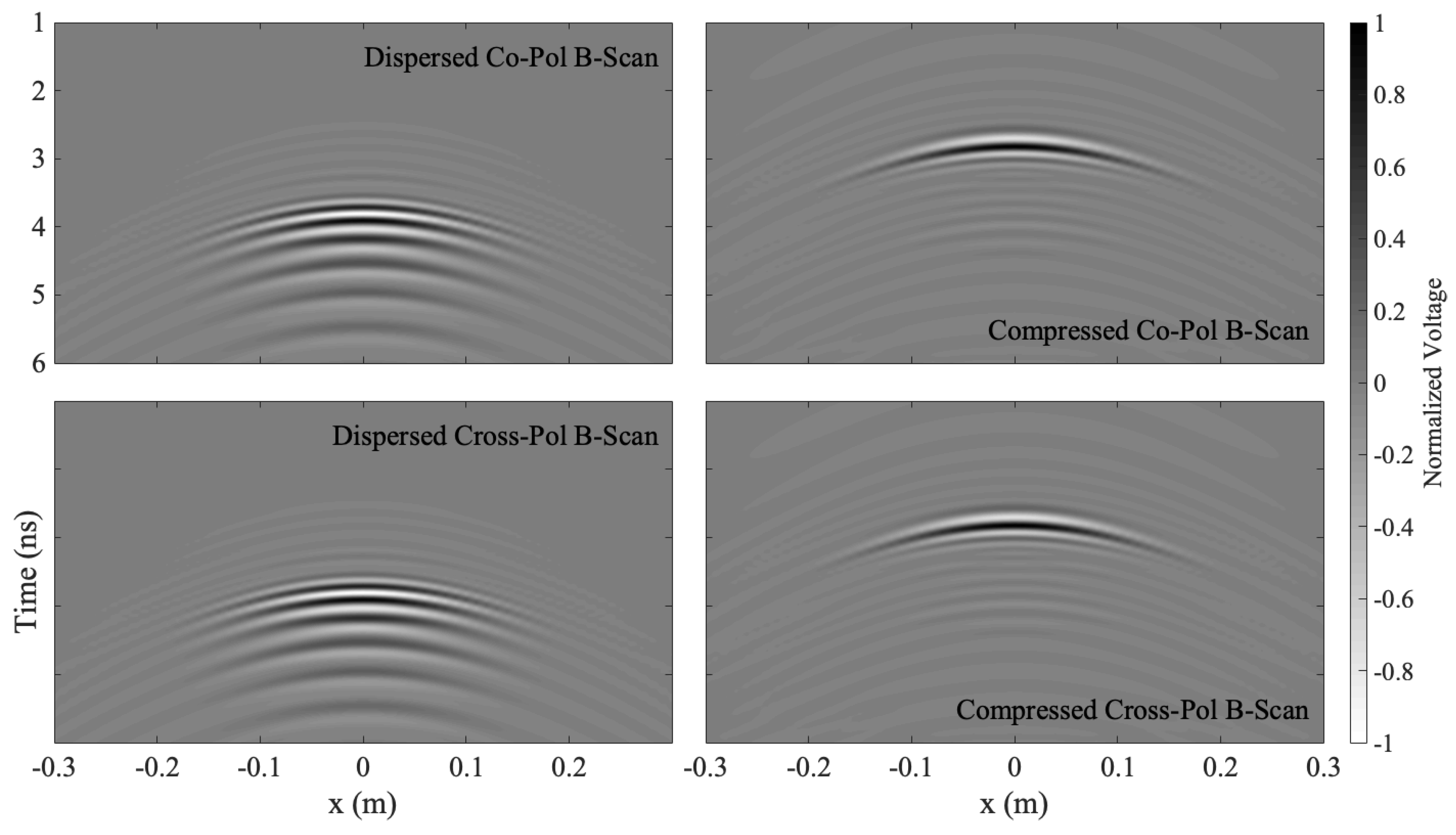
The dispersion model was applied to a simulated GPR scenario where the 16-cell () sinuous antenna was simulated over a dry sandy-soil half-space (CST Microwave Studio) as depicted by Figure 11. Each pair of antenna arms were excited individually in order to produce orthogonal senses of linear polarization i.e., and . The radiated electric field was probed at a 20 cm depth along the x-axis and used to compute the returned signal from a small linear scatter (3 cm long wire with a 1 mm radius) via the reciprocity model and polarizability tensor developed in [13]. Two orientations of the target were considered: first, the target was aligned at a 45° angle in the x–y plane to produce equal co-polarized and cross-polarized returns, and, second, the target was aligned at a 0° to produce only a co-polarized response. The resulting time-domain B-scans, both with and without dispersion compensation, for the cross-polarized and co-polarized targets are displayed in Figure 12 and Figure 13, respectively. The returns were normalized to the peak voltage for display purposes.
The optimized dispersion model from Table 1 was applied twice to the received voltage to compensate for dispersion produced during both transmit and receive. Results presented in Section 3.2 indicated the applicability of this dispersion model since the proximity of the dry sandy-soil produced only negligible effects on the antenna’s dispersion. As can be seen, the model can successfully correct the dispersed pulses both on and off-boresight, thereby significantly increasing the GPR’s range resolution. Furthermore, the dispersion model behaves as expected for both co-polarized and cross-polarized targets. This confirms the applicability of the model to sinuous antennas employed in polarimetric systems.
5. Limitations of the Log-Periodic Dispersion Model
The presented dispersion model is based on the assumption of log-periodic antenna operation. When the actual radiation from the antenna breaks this assumption, the dispersion model becomes invalid. This was evident for frequencies below the operating range of the antenna where the constant delay was applied to the dispersion model (see Figure 6). Another factor that reduces the effectiveness of the dispersion model is radiation from the bow-tie feed. A good guideline is to keep , for the highest frequency desired, to prevent such radiation. Reducing also results in small trace widths at the feed, which may be difficult to reliably manufacture. For this reason, some have proposed breaking the log-periodic nature of the sinuous by letting vary with the radius [32,33]. In this case, the model would need to be altered since the antenna is now quasi-log-periodic [7].
Another potential pitfall is the unintended excitation of resonant modes that produce sharp variations in gain and phase of the antenna over frequency [21]. This may occur if the sinuous antenna design parameters and outer truncation method are not properly selected [20]. The lower bound on the sinuous antenna operating frequency may be approximated as
where v is the wave velocity and and are specified in radians [7]. Such a relationship may encourage GPR antenna designers to choose larger values of for lower operating frequencies. However, large values of have been shown to result in undesired resonate modes excited between adjacent antenna arms; furthermore, the traditional truncation of sinuous antennas produces a sharp end that resonates at low frequencies [20,21]. These unintended resonate modes reduce the ability of simple dispersion models to accurately compensate for dispersion in radiated pulses.
In order to illustrate this, a traditionally truncated sinuous antenna with = 65° (see Figure 14) was simulated similarly to the antennas presented in Section 2. The group delay is shown in Figure 15 and displays sharp discontinuities resulting from the excitation of unintended resonant modes. The group delay computed from the corresponding dispersion model is also shown in Figure 15. The default model with a fixed delay cap of 4.7 ns at low frequencies is used here since the sharp discontinuities complicate improving the model with an optimized curve fit. The dispersion model is used to correct the radiated pulse as shown in Figure 16; it is not able to correct the ringing resulting from the unintended resonant modes since it no longer fully represents the group delay of the antenna. Thus, the sinuous antenna must be designed to mitigate such ringing, as outlined in [20], before the application of the simple log-periodic dispersion model.
6. Experimental Validation
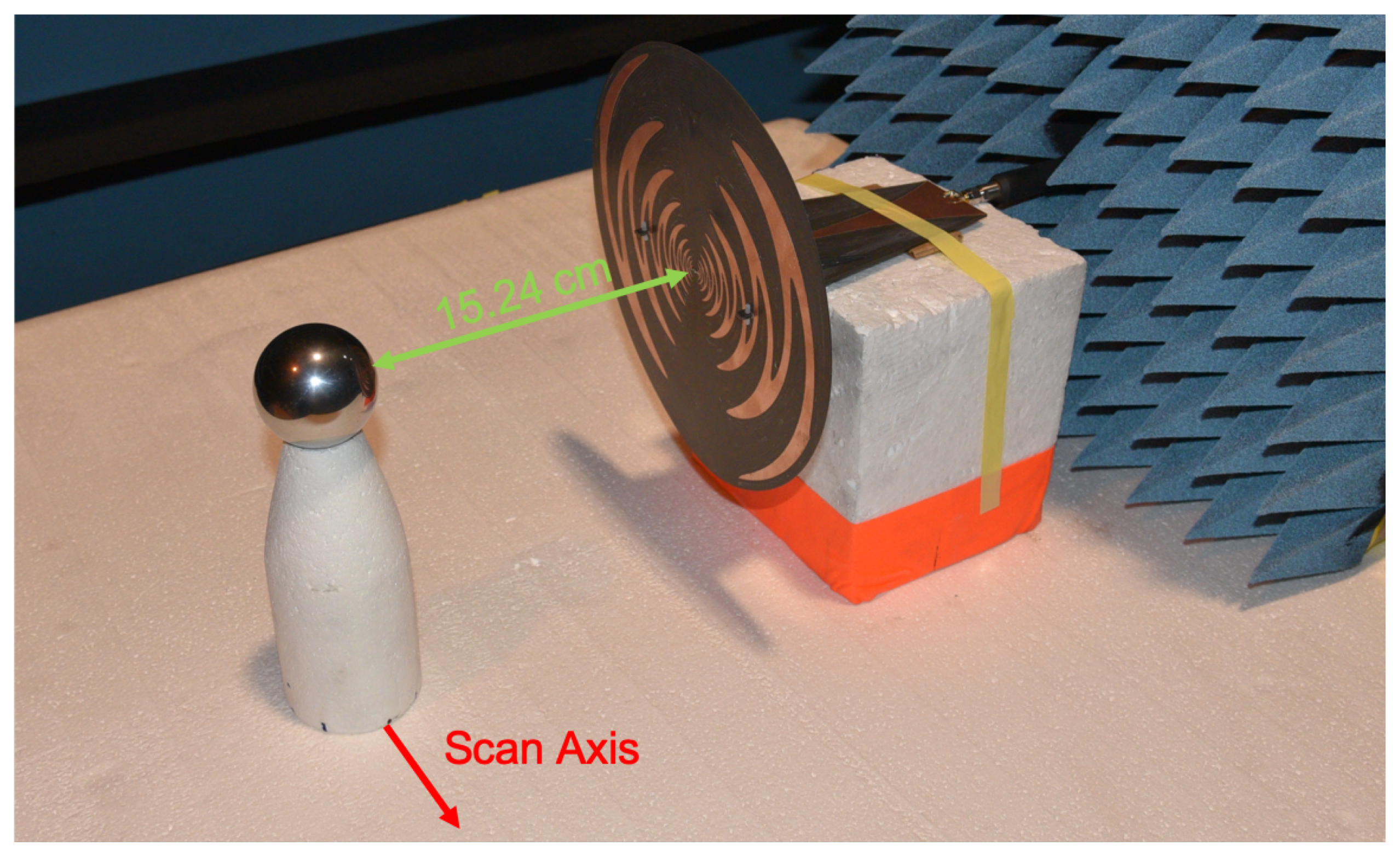
In order to validate the analysis presented above, the 16-cell antenna defined in Section 2 was fabricated and measured. The dispersive nature of the antenna was investigated by measuring the response from a 5.08 cm diameter sphere. The sphere was placed 15.24 cm from the antenna on boresight and then scanned perpendicular to the antenna another 15.24 cm in 1.27 cm increments. The fabricated antenna in the measurement setup is shown in Figure 17.
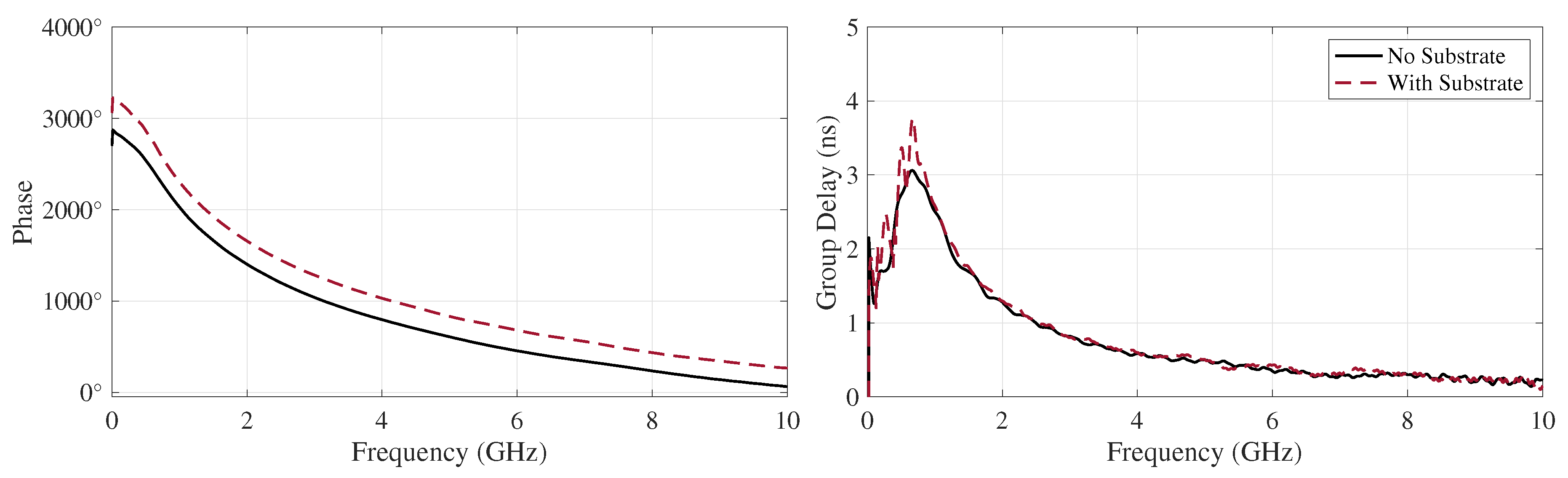
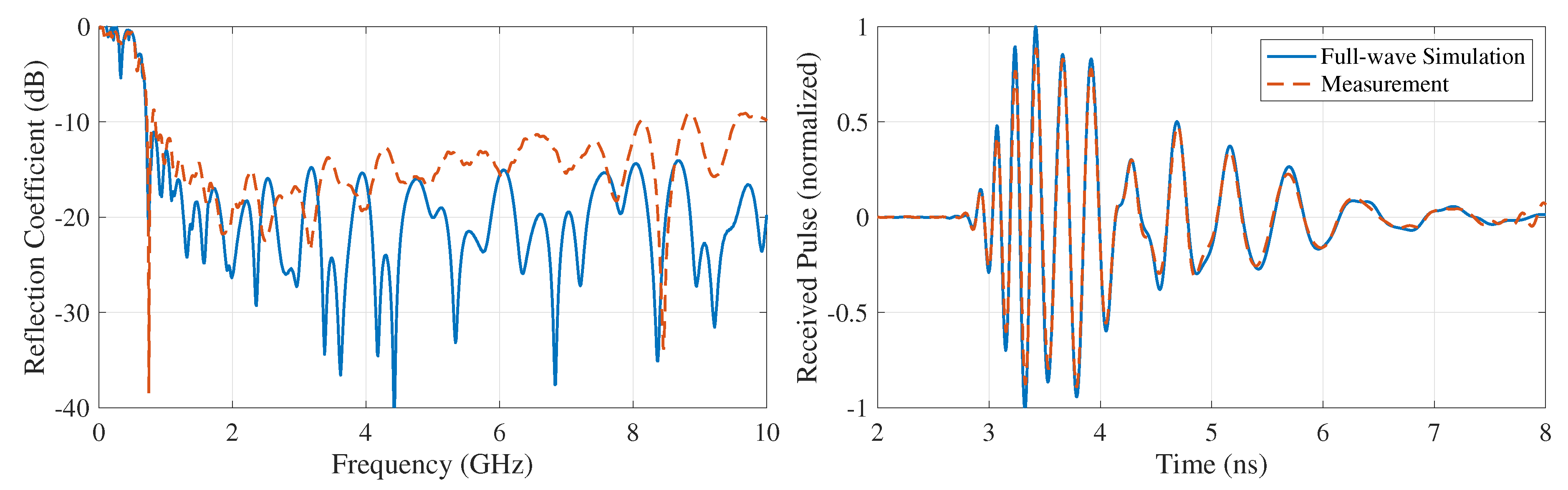
The antenna was manufactured using an LPKF circuit board milling machine [34] out of 0.031” Rogers RT/duroid® 5880 laminate (1 oz. copper clad) [35]. The 5880 material has very low loss (tan of 0.0009 at 10 GHz) and a relative permittivity of 2.20 [35]. Simulations showed the effect of the substrate on the antenna’s dispersion to be small (see Figure 18). As can be seen from Figure 17, each set of opposing sinuous arms were placed on opposite sides of the substrate. This was done to simplify feeding the antenna. Only a single pair of arms was fed by a tapered microstrip balun while the other pair of arms was terminated with a 221 chip resistor resulting in the antenna producing linear (horizontal) polarization [20,36,37]. Simulation results showed the presence of the substrate lowered the input impedance to approximately 230 (averaged over the band). The constructed balun was milled from 0.062” Rogers RT/duroid® 5880 laminate (0.5 oz. copper clad) and started as unbalanced 50 microstrip, which was then tapered over a 150 mm length to balanced parallel stripline. The top trace was tapered linearly while an exponential taper was used for the ground plane. The microstrip was fed by an SMA edge connector. For structural stability, triangular braces were included (also cut from the 5880 material) and the balun had tabs that extended through slots cut into the antenna substrate, allowing plastic pins to hold the parts together [20]. A detailed model of the measured antenna, including the balun and SMA transition, was developed in CST Microwave Studio and simulated using the time-domain solver. The simulated and measured reflection coefficient vs. frequency is compared in Figure 19. As can be seen, the simulated and measured results correlate quite well.
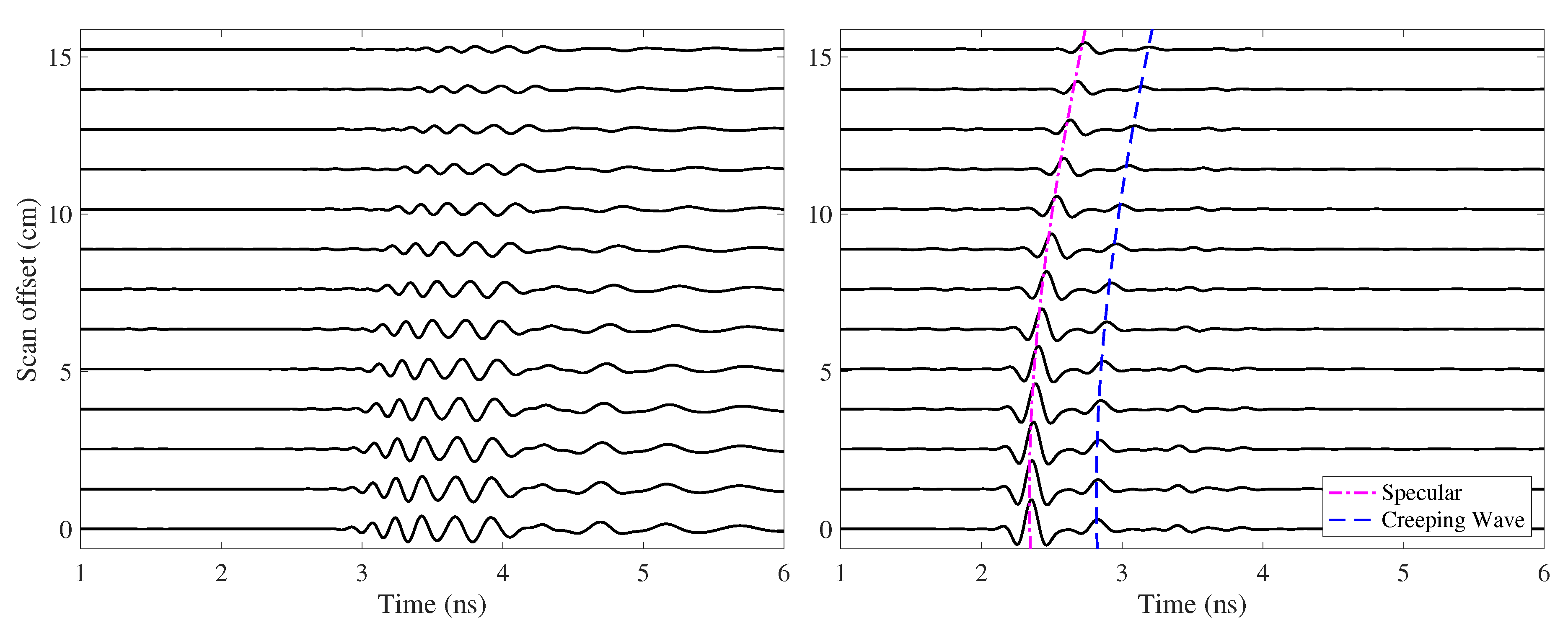
The target returns () were measured in the frequency domain from 10 MHz to 10 GHz with a vector network analyzer. The background, including the foam mast, was also measured at each scan location and subsequently removed from the target results by coherent subtraction. Note that the calibration plane is located at the SMA connection to the antenna; therefore, the time delay due to the balun is included in the results. The sans background target returns were then weighted by a Taylor window ( and ) [38] and transformed to the time domain via inverse fast Fourier transform (IFFT). The measurement setup, i.e., antenna and 2” sphere on boresight, were also simulated and the resulting received (dispersed) pulses are compared in Figure 19. The waterfall diagram in Figure 20 shows the processed time-domain responses for each scan location both with and without dispersion compensation. The dispersion model parameters were determined by an optimization process that maximized the cross-correlation of the boresight return with that of the time-domain window function i.e., the IFFT of the Taylor window. This was done to adjust the model for the presence of the substrate and feed. The optimized parameters were and GHz. As can be seen, identifying aspects of the target are indistinguishable before dispersion compensation. With the dispersion model applied, the specular and creeping wave returns from the sphere become clearly visible. The model is also able to successfully remove the dispersion for the off-boresight scan locations.
7. Conclusions
Sinuous antennas embody many characteristics that are advantageous to GPR applications e.g., ultra-wideband (UWB) radiation and polarization diversity. However, they are dispersive, which reduces effectiveness when radiating UWB pulses. In this work, a model was presented for the compensation of dispersion in log-periodic sinuous antennas, which is based on antenna design parameters and can be optimized for best fit. The model was shown to have application for different sinuous antenna designs as well as in the vicinity of different soils. Additionally, it was shown that care must be taken when designing sinuous antennas to ensure the applicability of such dispersion models i.e., preventing unintended resonant modes. Both numerical and experimental scenarios were investigated with the model successfully used to compensate sinuous antenna dispersion, thereby improving range resolution for polarimetric GPR applications. Such a model may have advantages over applying simulated or measured phase information since the model is simplistic and can be adjusted in the field to accommodate any changes in antenna performance due to the environment.
Funding
This work was supported in part by Sandia National Laboratories, a multimission laboratory managed and operated by National Technology and Engineering Solutions of Sandia, LLC., a wholly-owned subsidiary of Honeywell International, Inc., for the U.S. Department of Energy’s National Nuclear Security Administration under Contract DE-NA0003525. This paper describes objective technical results and analysis. Any subjective views or opinions that might be expressed in the paper do not necessarily represent the views of the U.S. Department of Energy or the United States Government.
Acknowledgments
The authors would like to thank Bernd Strassner II, Doug Brown, Diana Frederick, John Borchardt, Tyler LaPointe, Troy Satterthwait, Wade Freeman and Ward Patitz of Sandia National Laboratories for helpful discussion and feedback during the development of this manuscript as well as assistance in the use of the fabrication and measurement equipment.
Conflicts of Interest
The authors declare no conflicts of interest.
References
- Peters, L.P.; Daniels, J.J.; Young, J.D. Ground penetrating radar as a subsurface environmental sensing tool. Proc. IEEE 1994, 82, 1802–1822. [Google Scholar] [CrossRef]
- Krueger, K.R.; McClellan, J.H.; Scott, W.R. Efficient Algorithm Design for GPR Imaging of Landmines. IEEE Trans. Geosci. Remote Sens. 2015, 53, 4010–4021. [Google Scholar] [CrossRef]
- Daniels, D.J. (Ed.) Ground Penetrating Radar, 2nd ed.; Electromagnetics and Radar Series; Institution of Engineering and Technology: London, UK, 2004. [Google Scholar]
- MacDonald, J.; Lockwood, J.R. Alternatives for Landmine Detection; RAND Corporation: Santa Monica, CA, USA, 2003. [Google Scholar]
- Giuli, D. Polarization diversity in radars. Proc. IEEE 1986, 74, 245–269. [Google Scholar] [CrossRef]
- Yu, Y.; Chen, C.C.; Feng, X.; Liu, C. Application of entropy classification method to the detection of subsurface linear targets in polarimetric GPR data. In Proceedings of the 2016 IEEE International Geoscience and Remote Sensing Symposium (IGARSS), Beijing, China, 10–15 July 2016; pp. 7438–7441. [Google Scholar]
- DuHamel, R.H. Dual Polarized Sinuous Antennas. U.S. Patent 4,658,262, 14 April 1987. [Google Scholar]
- Blejer, D.J.; Scarborough, S.M.; Frost, C.E.; Catalan, H.R.; McCoin, K.H.; Roman, J.; Mukai, D.M. Ultra-wideband polarimetric imaging of corner reflectors in foliage. In Proceedings of the IEEE Antennas and Propagation Society International Symposium 1992 Digest, Chicago, IL, USA, 18–25 June 1992; Volume 1, pp. 587–590. [Google Scholar] [CrossRef]
- Pochanin, G.P.; Kaluzhny, N.M.; Masalov, S.A.; Pochanina, I.Y. Ultrawideband linearly polarized antennas of Vivaldi type for ground penetrating radar. In Proceedings of the 2015 International Conference on Antenna Theory and Techniques (ICATT), Kharkiv, Ukraine, 21–24 April 2015; pp. 1–3. [Google Scholar] [CrossRef]
- Sustman, J.W.; Scott, W.R. A resistive-vee dipole based polarimetric antenna. In Proceedings of the 2013 IEEE Antennas and Propagation Society International Symposium (APSURSI), Orlando, FL, USA, 7–13 July 2013; pp. 888–889. [Google Scholar] [CrossRef]
- Feng, X.; Sato, M.; Liu, C. Subsurface Imaging Using a Handheld GPR MD System. IEEE Geosci. Remote Sens. Lett. 2012, 9, 659–662. [Google Scholar] [CrossRef]
- McMichael, I.T.; Scott, W.R.; Nallon, E.C.; Schnee, V.P.; Mirotznik, M.S. EBG antenna for GPR co-located with a metal detector for landmine detection. In Proceedings of the 2013 IEEE International Geoscience and Remote Sensing Symposium—IGARSS, Melbourne, Australia, 21–26 July 2013; pp. 3915–3918. [Google Scholar] [CrossRef]
- McFadden, M. Analysis of the Equiangular Spiral Antenna. Ph.D. Thesis, School of Electrical and Computer Engineering, Georgia Institute of Technology, Atlanta, GA, USA, 2009. Available online: https://smartech.gatech.edu/handle/1853/31726 (accessed on 18 August 2019).
- Hertel, T.W.; Smith, G.S. On the dispersive properties of the conical spiral antenna and its use for pulsed radiation. IEEE Trans. Antennas Propag. 2003, 51, 1426–1433. [Google Scholar] [CrossRef]
- Knop, C. On transient radiation from a log-periodic dipole array. IEEE Trans. Antennas Propag. 1970, 18, 807–808. [Google Scholar] [CrossRef]
- McLean, J.; Foltz, H.; Sutton, R. The quantitative assessment of the UWB performance of log-periodic dipole antennas with fixed equalization. In Proceedings of the 2004 International Workshop on Ultra Wideband Systems Joint with Conference on Ultra Wideband Systems and Technologies, Joint UWBST IWUWBS 2004 (IEEE Cat. No.04EX812), Kyoto, Japan, 18–21 May 2004; pp. 317–321. [Google Scholar] [CrossRef]
- Olvera, A.D.J.F.; Nandi, U.; Norman, J.; Gossard, A.C.; Roskos, H.; Preu, S. Dispersive properties of self-complementary log-periodic antennas in pulsed THz systems. In Proceedings of the 2017 42nd International Conference on Infrared, Millimeter, and Terahertz Waves (IRMMW-THz), Cancun, Mexico, 27 August–1 September 2017; pp. 1–2. [Google Scholar] [CrossRef]
- Bradley, M.R.; Witten, T.R.; Duncan, M.; McCummins, R. Mine detection with a forward-looking ground-penetrating synthetic aperture radar. In Proceedings of the Detection and Remediation Technologies for Mines and Minelike Targets VIII, International Society for Optics and Photonics, Orlando, FL, USA, 11 September 2003; Volume 5089. [Google Scholar] [CrossRef]
- Clark, W.W.; Lacko, P.R.; Ralston, J.M.; Dieguez, E. Wideband 3D imaging radar using Archimedean spiral antennas. In Proceedings of the Detection and Remediation Technologies for Mines and Minelike Targets VIII, International Society for Optics and Photonics, Orlando, FL, USA, 11 September 2003; Volume 5089. [Google Scholar]
- Crocker, D.; Scott, W. On the Design of Sinuous Antennas for UWB Radar Applications. IEEE Antennas Wirel. Propag. Lett. 2019, 18, 1347–1351. [Google Scholar] [CrossRef]
- Kang, Y.; Kim, K.; Scott, W.R. Modification of Sinuous Antenna Arms for UWB Radar Applications. IEEE Trans. Antennas Propag. 2015, 63, 5229–5234. [Google Scholar] [CrossRef]
- Sower, G.D.; Kilgore, R.; Roman, J.R. GSTAMIDS ground-penetrating radar: Data processing algorithms. In Proceedings of the Detection and Remediation Technologies for Mines and Minelike Targets VI, International Society for Optics and Photonics, Orlando, FL, USA, 18 October 2001; Volume 4394. [Google Scholar] [CrossRef]
- Jin, T.; Zhou, Z. Refraction and Dispersion Effects Compensation for UWB SAR Subsurface Object Imaging. IEEE Trans. Geosci. Remote Sens. 2007, 45, 4059–4066. [Google Scholar] [CrossRef]
- DuHamel, R.; Isbell, D. Broadband logarithmically periodic antenna structures. In Proceedings of the 1958 IRE International Convention Record, New York, NY, USA, 21–25 March 1966; Volume 5, pp. 119–128. [Google Scholar] [CrossRef]
- Edwards, J.M.; O’Brient, R.; Lee, A.T.; Rebeiz, G.M. Dual-Polarized Sinuous Antennas on Extended Hemispherical Silicon Lenses. IEEE Trans. Antennas Propag. 2012, 60, 4082–4091. [Google Scholar] [CrossRef]
- Baldonero, P.; Manna, A.; Trotta, F.; Pantano, A.; Bartocci, M. UWB Double polarised phased array. In Proceedings of the 2009 3rd European Conference on Antennas and Propagation, Berlin, Germany, 23–27 March 2009; pp. 556–560. [Google Scholar]
- Dassault Systèmes. CST STUDIO SUITE 2018. Available online: https://www.3ds.com/products-services/simulia/products/cst-studio-suite (accessed on 25 July 2019).
- Weisstein, E.W. Gaussian Function. From MathWorld—A Wolfram Web Resource. Available online: http://mathworld.wolfram.com/GaussianFunction.html (accessed on 25 July 2019).
- Weisstein, E.W. Hermite Polynomial. From MathWorld—A Wolfram Web Resource. Available online: http://mathworld.wolfram.com/HermitePolynomial.html (accessed on 25 July 2019).
- Lee, S. Approximation of Gaussian by Scaling Functions and Biorthogonal Scaling Polynomials. Bull. Malays. Math. Sci. Soc. 2009, 32. [Google Scholar]
- The MathWorks, Inc. MATLAB R2018 Optimization Toolbox. Available online: https://www.mathworks.com/products/optimization.html (accessed on 25 July 2019).
- Sammeta, R.; Filipovic, D. Quasi-frequency independent high power sinuous antenna. In Proceedings of the 2012 IEEE International Symposium on Antennas and Propagation, Chicago, IL, USA, 8–14 July 2012; pp. 1–2. [Google Scholar] [CrossRef]
- Sammeta, R.; Filipovic, D.S. Improved Efficiency Lens-Loaded Cavity-Backed Transmit Sinuous Antenna. IEEE Trans. Antennas Propag. 2014, 62, 6000–6009. [Google Scholar] [CrossRef]
- LPKF Laser & Electronics AG. LPKF Laser & Electronics. Available online: https://www.lpkf.com/en/ (accessed on 29 January 2019).
- Rogers Corporation. RT/duroid 5880 Laminates. Available online: http://www.rogerscorp.com/acs/products/32/rt-duroid-5880-laminates.aspx (accessed on 29 January 2019).
- Lorho, N.; Lirzin, G.; Bikiny, A.; Lestieux, S.; Chousseaud, A.; Razban, T. Miniaturization of an UWB Dual-Polarized Antenna. In Proceedings of the 2015 IEEE International Conference on Ubiquitous Wireless Broadband (ICUWB), Montreal, QC, Canada, 4–7 October 2015; pp. 1–5. [Google Scholar]
- Aghdam, K.M.P.; Faraji-Dana, R.; Rashed-Mohassel, J. Optimization of microstrip tapered balun for sinuous antenna feeding circuits. In Proceedings of the 2004 10th International Symposium on Antenna Technology and Applied Electromagnetics and URSI Conference, Ottawa, ON, Canada, 20–23 July 2004; pp. 1–4. [Google Scholar] [CrossRef]
- Richards, M.A.; Sheer, J.A.; Holm, W.A. (Eds.) Principles of Modern Radar; SciTech: Edison, NJ, USA, 2010; Volume 1, pp. 797–800. [Google Scholar]
Figure 1.
Sinuous antennas having parameters: cells, (left); cells, (center); and cells, (right). Other parameters constant for all antennas: arms, cm, cm, = 45°, and = 22.5°.
Figure 1.
Sinuous antennas having parameters: cells, (left); cells, (center); and cells, (right). Other parameters constant for all antennas: arms, cm, cm, = 45°, and = 22.5°.

Figure 2.
Illustration of the sinuous antenna active region as described in the original patent [7].
Figure 2.
Illustration of the sinuous antenna active region as described in the original patent [7].

Figure 3.
Illustration of sinuous antenna design parameters: angular width , expansion ratio , outermost cell radius , and curve rotation angle .
Figure 3.
Illustration of sinuous antenna design parameters: angular width , expansion ratio , outermost cell radius , and curve rotation angle .

Figure 4.
Reflection coefficient and boresight realized gain vs. frequency for the sinuous antennas investigated.
Figure 4.
Reflection coefficient and boresight realized gain vs. frequency for the sinuous antennas investigated.

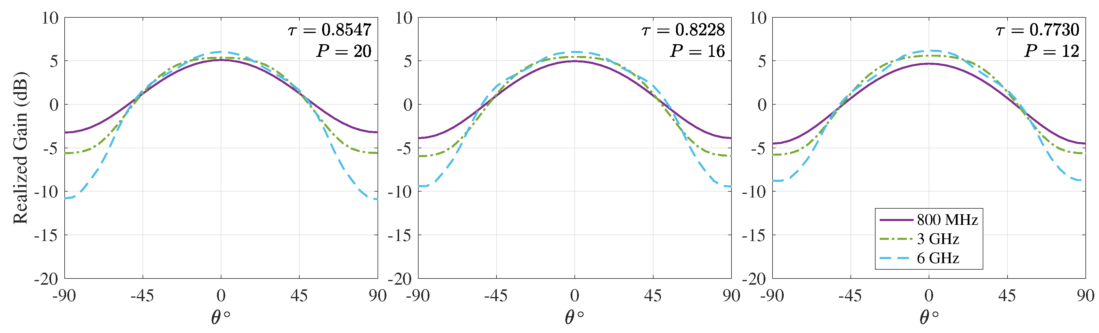
Figure 5.
Principle E-plane pattern cuts at 800 MHz, 3 GHz, and 5 GHz for the sinuous antennas investigated.
Figure 5.
Principle E-plane pattern cuts at 800 MHz, 3 GHz, and 5 GHz for the sinuous antennas investigated.

Figure 6.
Full-wave simulation vs. simple model of both phase (left) and group delay (right) due to dispersion in the 20, 16, and 12 cell sinuous antennas. Note that phase unwrapping starts at 10 GHz.
Figure 6.
Full-wave simulation vs. simple model of both phase (left) and group delay (right) due to dispersion in the 20, 16, and 12 cell sinuous antennas. Note that phase unwrapping starts at 10 GHz.

Figure 7.
Double-differentiated Gaussian pulse used as the voltage excitation to compute the radiated pulses from the simulated electric field data using Equation (4). The time-domain representation of the signal (left) shows a peak amplitude of 1 V at 0.36 ns, while in the frequency-domain (right) the signal has maximum spectral energy at 3 GHz.

Figure 8.
Dispersed radiated pulses at 2 m on boresight (left), and the corrected radiated pulse at 2 m on boresight after the simple antenna dispersion model has been applied (right).
Figure 8.
Dispersed radiated pulses at 2 m on boresight (left), and the corrected radiated pulse at 2 m on boresight after the simple antenna dispersion model has been applied (right).

Figure 9.
Radiated pulses from the 16-cell antenna at 20 cm boresight depth and three perpendicular scan locations: 0, 10, 20 cm. The pulses are shown both before (left) and after (right) application of the optimized simple antenna dispersion model listed in Table 1.
Figure 9.
Radiated pulses from the 16-cell antenna at 20 cm boresight depth and three perpendicular scan locations: 0, 10, 20 cm. The pulses are shown both before (left) and after (right) application of the optimized simple antenna dispersion model listed in Table 1.

Figure 10.
Boresight radiated pulses at 5 cm depth in three different materials: air, dry sand, and wet sand. The pulses are shown both before (left) and after (right) application of the dispersion model. The wet sand was highly lossy and dispersive, resulting in significantly smaller pulses and less effective pulse correction when using only the simple dispersion model for the antenna.

Figure 11.
Illustration of the GPR simulation: the sinuous antenna is simulated over a lossy soil half-space containing field probes at a depth of 20 cm. The target response at each field-probe location was determined with a reciprocity model.
Figure 11.
Illustration of the GPR simulation: the sinuous antenna is simulated over a lossy soil half-space containing field probes at a depth of 20 cm. The target response at each field-probe location was determined with a reciprocity model.

Figure 12.
GPR simulation results: dispersed co-pol and cross-pol B-scans (left) and corrected B-scans using an optimized dispersion model (right) for a small linear target aligned at a 45° angle to the incident wave polarization.
Figure 12.
GPR simulation results: dispersed co-pol and cross-pol B-scans (left) and corrected B-scans using an optimized dispersion model (right) for a small linear target aligned at a 45° angle to the incident wave polarization.

Figure 13.
GPR simulation results: dispersed co-pol and cross-pol B-scans (left) and corrected B-scans using an optimized dispersion model (right) for a small linear target aligned with the incident wave polarization.
Figure 13.
GPR simulation results: dispersed co-pol and cross-pol B-scans (left) and corrected B-scans using an optimized dispersion model (right) for a small linear target aligned with the incident wave polarization.

Figure 14.
Traditional sinuous antenna having parameters: arms, cells, cm, , = 65°, and = 22.5°. This antenna exhibits sharp discontinuities in the gain due to unintended resonate modes.
Figure 14.
Traditional sinuous antenna having parameters: arms, cells, cm, , = 65°, and = 22.5°. This antenna exhibits sharp discontinuities in the gain due to unintended resonate modes.

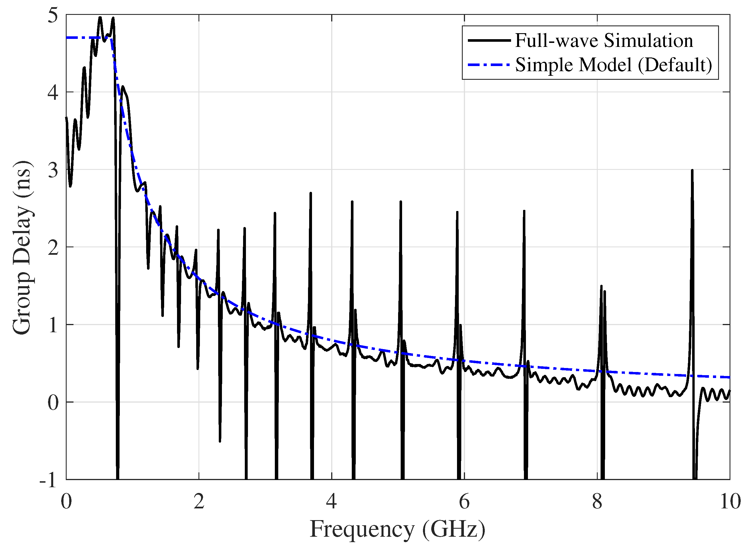
Figure 15.
Full-wave simulation vs. simple model (default parameters with fixed delay cap ) of the group delay due to dispersion in the traditional sinuous antenna with resonances.
Figure 15.
Full-wave simulation vs. simple model (default parameters with fixed delay cap ) of the group delay due to dispersion in the traditional sinuous antenna with resonances.

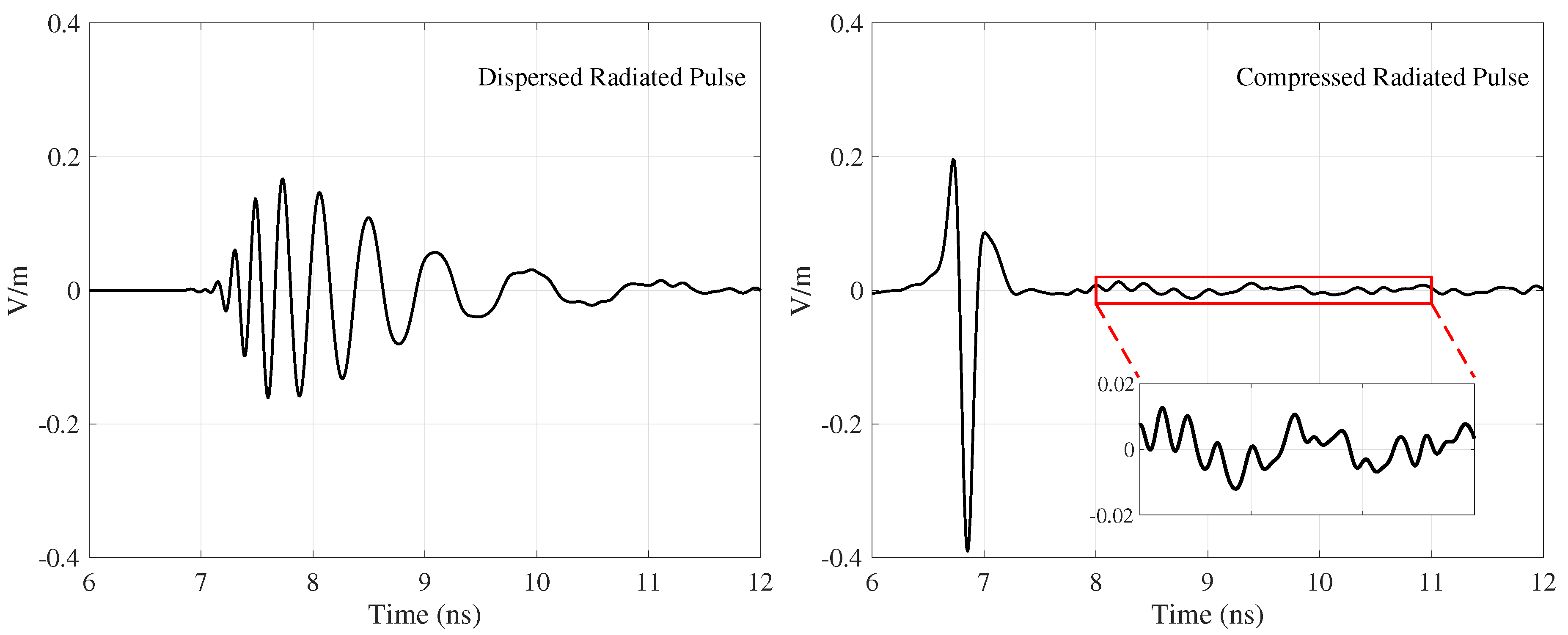
Figure 16.
Dispersed radiated pulse at 2 m (left), and the corrected radiated pulse at 2 m after the dispersion model has been applied (right) for the traditional sinuous antenna with resonances. Note that the dispersion model does not compensate for the late-time ringing due to the unintended resonant modes.

Figure 17.
Setup of the validation measurement showing the fabricated 16-cell sinuous antenna and the 5.08 cm spherical target at the boresight scan location.
Figure 17.
Setup of the validation measurement showing the fabricated 16-cell sinuous antenna and the 5.08 cm spherical target at the boresight scan location.

Figure 18.
Full-wave simulations of the 16-cell antenna’s phase (left) and group delay (right) due to dispersion both with and without the inclusion of a substrate. Note that phase unwrapping starts at 10 GHz.
Figure 18.
Full-wave simulations of the 16-cell antenna’s phase (left) and group delay (right) due to dispersion both with and without the inclusion of a substrate. Note that phase unwrapping starts at 10 GHz.

Figure 19.
Full-wave simulation vs. measurement of the 16-cell antenna with tapered balun feed. Reflection coefficient comparison (left) and 2” sphere target return pulse (right).
Figure 19.
Full-wave simulation vs. measurement of the 16-cell antenna with tapered balun feed. Reflection coefficient comparison (left) and 2” sphere target return pulse (right).

Figure 20.
Waterfall plot of measured B-scan showing the dispersed (left) and corrected (right) time-domain responses from the measured 5.08 cm sphere. Both the specular and creeping wave reflections (denoted by the hyperbolic curves) are evident in the corrected results. Note that the results also contain the time delay due to the balun.


Table 1.
Log-periodic dispersion model parameters from Equation (6) and optimized versions for the three different sinuous antennas investigated.
Table 1.
Log-periodic dispersion model parameters from Equation (6) and optimized versions for the three different sinuous antennas investigated.
| Antenna Parameters | Default Model Parameters | Optimized Model Parameters | |||||
|---|---|---|---|---|---|---|---|
| P | (rad) | (GHz) | (ns) | (rad) | (GHz) | (ns) | |
| 20 | 0.8547 | 20.01 | 10.0 | N/A | 18.38 | 10.8 | 3.7 |
| 16 | 0.8228 | 16.11 | 10.0 | N/A | 14.82 | 10.4 | 3.0 |
| 12 | 0.7730 | 12.20 | 10.0 | N/A | 11.28 | 9.77 | 2.5 |
© 2019 by the authors. Licensee MDPI, Basel, Switzerland. This article is an open access article distributed under the terms and conditions of the Creative Commons Attribution (CC BY) license (http://creativecommons.org/licenses/by/4.0/).
Share and Cite
MDPI and ACS Style
Crocker, D.A.; Scott, W.R., Jr. Compensation of Dispersion in Sinuous Antennas for Polarimetric Ground Penetrating Radar Applications. Remote Sens. 2019, 11, 1937. https://0-doi-org.brum.beds.ac.uk/10.3390/rs11161937
AMA Style
Crocker DA, Scott WR Jr. Compensation of Dispersion in Sinuous Antennas for Polarimetric Ground Penetrating Radar Applications. Remote Sensing. 2019; 11(16):1937. https://0-doi-org.brum.beds.ac.uk/10.3390/rs11161937
Chicago/Turabian StyleCrocker, Dylan A., and Waymond R. Scott, Jr. 2019. "Compensation of Dispersion in Sinuous Antennas for Polarimetric Ground Penetrating Radar Applications" Remote Sensing 11, no. 16: 1937. https://0-doi-org.brum.beds.ac.uk/10.3390/rs11161937
Note that from the first issue of 2016, this journal uses article numbers instead of page numbers. See further details here.