Spatial Variation of NO2 and Its Impact Factors in China: An Application of Sentinel-5P Products


1
School of Geographical Sciences, Guangzhou University, Guangzhou 510006, China
2
Department of Land, Environment, Agriculture and Forestry, University of Padova, 35020 Padova, Italy
3
Guangdong Province Engineering Technology Research Center for Geographical Conditions Monitoring and Comprehensive Analysis, Guangzhou 510006, China
*
Author to whom correspondence should be addressed.
Remote Sens. 2019, 11(16), 1939; https://0-doi-org.brum.beds.ac.uk/10.3390/rs11161939
Submission received: 30 June 2019
/
Revised: 8 August 2019
/
Accepted: 9 August 2019
/
Published: 19 August 2019
(This article belongs to the Special Issue Innovative Remote Sensing for Monitoring and Assessment of Natural Resources)
Abstract
:As an important tropospheric trace gas and precursor of photochemical smog, the accumulation of NO2 will cause serious air pollution. China, as the largest developing country in the world, has experienced a large amount of NO2 emissions in recent decades due to the rapid economic growth. Compared with the traditional air pollution monitoring technology, the rapid development of the remote sensing monitoring method of atmospheric satellite has gradually become the critical technical means of global atmospheric environmental monitoring. To reveal the NO2 pollution situation in China, based on the latest NO2 products from Sentinel-5P TROPOMI, the spatial–temporal characteristics and impact factors of troposphere NO2 column concentration of mainland China in the past year (February 2018 to January 2019) were analyzed on two administrative levels for the first time. Results show that the monthly fluctuation of tropospheric NO2 column concentration has obvious characteristics of “high in winter and low in summer”, while the spatial distribution forms a “high in East and low in west” pattern, bounded by Hu Line. The comparison of Coefficient of Variation (CV) and spatial autocorrelation models at two kinds of administrative scales indicates that although the spatial heterogeneity of NO2 column concentration is less affected by the observed scale, there is a “delayed effect” of about one month in the process of NO2 column concentration fluctuation. Besides, the impact factors analysis based on Spatial Lag Model (SLM) and Geographic Weighted Regression (GWR) reveals that there is a positive correlation between nighttime light intensity, the secondary and tertiary industries proportion and NO2 column concentration. Furthermore, for regions with serious NO2 pollution in North China Plain, the whole society electricity consumption and vehicle ownership also play a positive role in increasing the NO2 column concentration. This study will enlighten the government and policy makers to formulate policies tailored to local conditions, to more effectively implement NO2 emission reduction and air pollution prevention.
1. Introduction
In the past decades, concomitant with the rapid process of industrialization and urbanization, China’s urban construction and socioeconomic development have made remarkable achievements [1]. At present, China has become the world’s most populous country with the second largest economy in the world, especially for eastern China, which has become one of the areas with the most intensive and intense human activities. However, the large-scale urban construction, urban population aggregation, and the rapid growth of the number of motor vehicles accompanied by urban development have led to the deterioration of air quality in urban areas of China, which not only reduces the visibility of the urban atmosphere, but also causes great harm to human health, thus threatening the sustainable development of economy and society. Among the various atmospheric pollutants, the large-scale emission of NOX (mainly including NO2 and NO) in China makes the concentration and growth rate of NO2 in the troposphere at a higher level, which is much higher than other countries and regions [2,3,4,5,6]. As an important trace gas, NO2 is mainly distributed in the troposphere and stratosphere, and plays an important role in the stratospheric and tropospheric atmospheric chemistry. NO2 is not only the main air pollution gas, but also an important precursor of ozone, acid rain, and photochemical smog. The nitrate aerosols produced by NO2 have significant radiation forcing, which makes NO2 an important factor in climate change [7]. Especially, since the middle of the 20th century, the emission of NO2 has increased dramatically, and the concentration of NO2 in the atmosphere has also increased continuously, which has a great negative impact on human health, ecological environment, biochemical cycle, tropospheric atmospheric composition, and air quality [8,9,10,11].
Generally, the sources of NO2 in the atmosphere mainly include natural and anthropogenic emissions [7]. Among them, the natural emission sources mainly include natural combustion of biomass, atmospheric lightning process, and nitrates of microbial action; while artificial emission sources mainly include agricultural burning, burning of fossil fuels, industrial production, and vehicle exhaust emissions [12,13,14,15]. However, with the development of human society, industrial thermal power and motor vehicle emissions have gradually become the main sources of nitrogen oxides, accounting for 90% of the total emissions [16]. At present, the anthropogenic emission of NO2 is mainly in the troposphere, and the concentration and fluctuation trend of NO2 in the stratosphere is smaller than that of the troposphere [17], mainly from the conversion of N2O and the direct emission of supersonic aircraft [18]. Hence, the higher the regional human activity intensity, the more drastic the change of tropospheric NO2 column concentration [19,20,21]. For years, the emission of NOX in China’s atmosphere has increased significantly, and the pollution of NOX has been deteriorating due to excessive coal combustion, lack of emission reduction measures, and the sharp increase of motor vehicle emissions.
Nowadays, the concentration of NO2 in the atmosphere has become one of the common indicators to measure the intensity of air pollution [22]. The study of temporal and spatial variations of NO2 and its influencing factors has become a hot topic in the study of atmospheric composition and trace gases. Since satellite remote sensing can efficiently and dynamically monitor the trend and distribution characteristics of gas pollutants, it has gradually become the key means for long-term large-scale monitoring of atmospheric changes in recent years [23,24,25,26,27,28]. The study of atmospheric trace gases by using remote sensing monitoring technology of atmospheric satellite began in the 1970s. In 1978, the United States carried a Total Ozone Mapping Spectrometer (TOMS) sensor on the Nimbus-7 satellite to monitor the total ozone change, marking the beginning of the formal study of tropospheric trace gases by satellite remote sensing [29]. Then, the ERS-2 satellite launched by European Space Agency (ESA) in 1995 was loaded with Global Ozone Monitoring Experiment (GOME), which was used to monitor the global distribution of trace gases [30]. In 2002, ENVISAT-1, launched by ESA, was loaded with three detectors Global Ozone Monitoring by Occultation of Stars (GOMOS), Moderate Resolution Imaging Spectroradiometer (MODIS), and SCanning Imaging Absorption SpectroMeter for Atmospheric CHartographY (SCIAMACHY), which were used to study the composition changes of HNO3, CH4, H2, N2O, Chlorofluorocarbon (CFC) and to detect the concentration distribution of aerosol and ozone layer [31]. In 2004, the Ozone Monitor (OMI) on NASA’s Earth Observation System (EOS) satellite Aura was able to obtain the global distribution of trace gases such as O3, NO2, and SO2 [32]. Subsequently, as the new-generation European instruments carried on MetOp series satellites, the Global Ozone Monitoring Experiment-2 (GOME-2) provides unique and long data sets for Atmospheric Research and application by measuring ozone, trace gases, and ultraviolet radiation [33,34].
However, the in-depth study of NO2 monitoring and analysis has prompted scholars to put forward higher requirements for the quality and resolution of satellite monitoring data. Meanwhile, in order to compensate for the data gap between the existing SCIAMACHY detector and the subsequent launch of Sentinel-5, the new Tropospheric Monitoring Instrument (TROPOMI) was loaded onboard the Sentinel-5 satellite for fine gas monitoring [35]. The core mission of the project is to monitor global-scale air quality, climate, and ozone layer from 2017 to 2023, providing better data support for scholars’ research on NO2 [36]. As a first imaging spectrometer to provide global data in medium spatial resolution, TROPOMI has a significant advantage over the previous sensor in spatial resolution (7 x 3.5km) and number of clear-sky observations per day [37]. Considering that the application and analysis of data products for Sentinel-5P are constantly improving, this paper selects the latest Sentinel-5P NO2 data product as data source, and synthesizes the distribution data of tropospheric NO2 column concentration in China [38]. Moreover, based on the spatial statistical analysis model, the distribution characteristics and impact factors of NO2 column concentration in the troposphere of China are analyzed and modeled, which can reveal the variation characteristics of NO2 and the source of pollutants, and provide suggestions for the designation of air quality control policies.
2. Study Area
The economic and urban development of China, as the largest and most representative developing country in the world, has achieved remarkable results since the 1980s with the implementation of the market economy and the reform of the economic system. In 2018, China’s Gross Domestic Product (GDP) reached 90.03 trillion yuan, which has become the second largest economy in the world after the United States and one of the fastest growing economies in the world. Meanwhile, the rapid development of China’s economy, the surge of urban population, and the increase of car ownership have led to a sharp increase in NO2 emissions, and the growth rate is much higher than that of other countries [6,39,40].
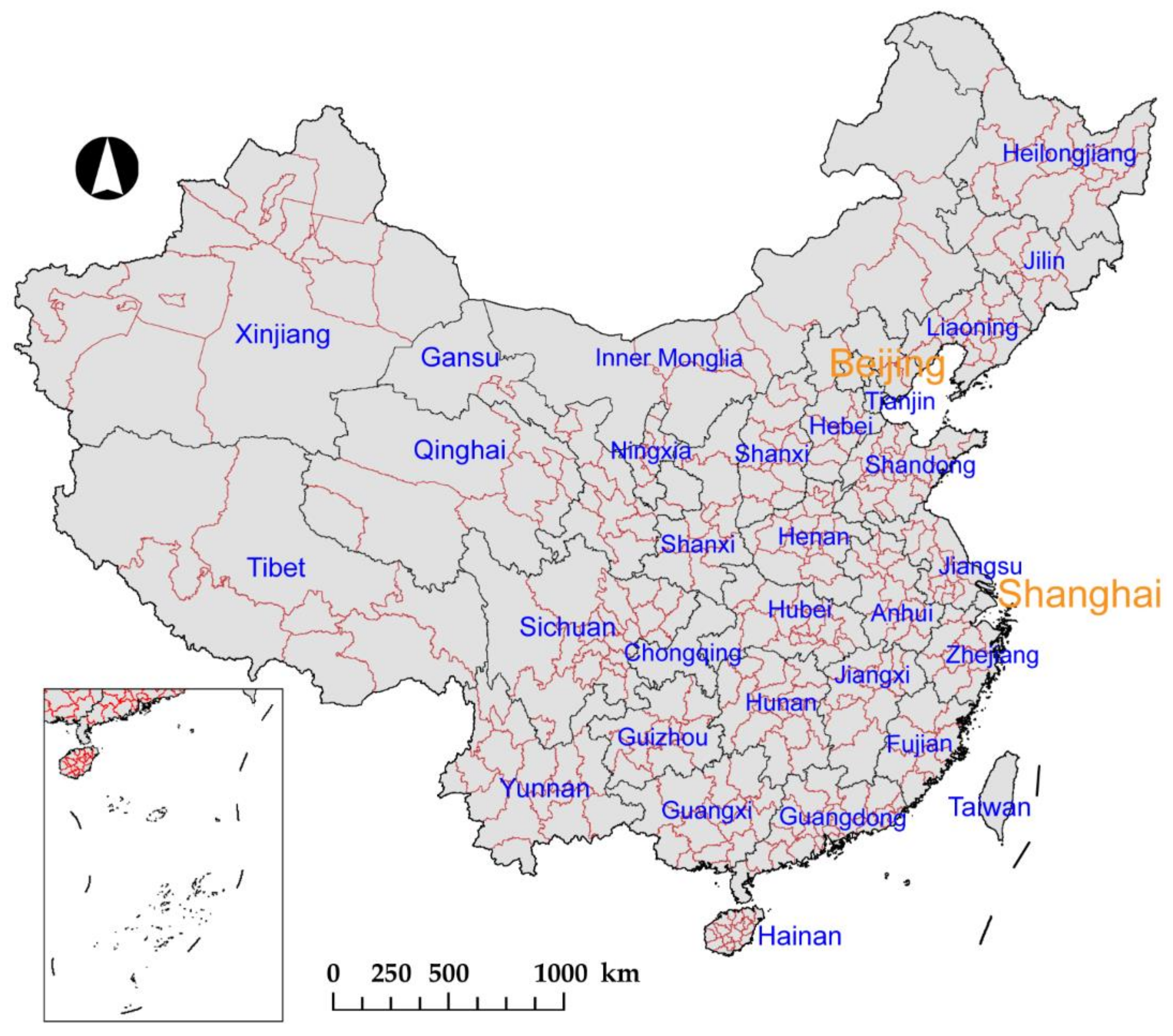
Due to its large population and vast territory, the administrative regionalization of China has a spatial stratification structure. The social and economic policies formulated or promulgated by the central government can be conveyed through the governments at the provincial, state, county, town, and village levels [41]. Since the 21st century, the number of prefecture level units in mainland China has gradually stabilized. As of October 2017, there are 334 prefecture-level administrative units in China, including: prefecture-level cities (294), autonomous prefectures (30), regions (7), and alliances (3). Since the provincial and prefectural units are the most representative and basic administrative units in China’s policy implementation, this paper selects them as the spatial units for NO2 spatial differentiation analysis (Figure 1). In addition, the statistics released by the Chinese government, including GDP, population, energy consumption, etc., are published on the basis of administrative divisions. Therefore, the spatial analysis with these two levels was carried out, which minimized the difficulty of collecting and sorting multidimensional socioeconomic data.
3. Materials and Methods
3.1. Data Collection
3.1.1. Remote Sensing Images
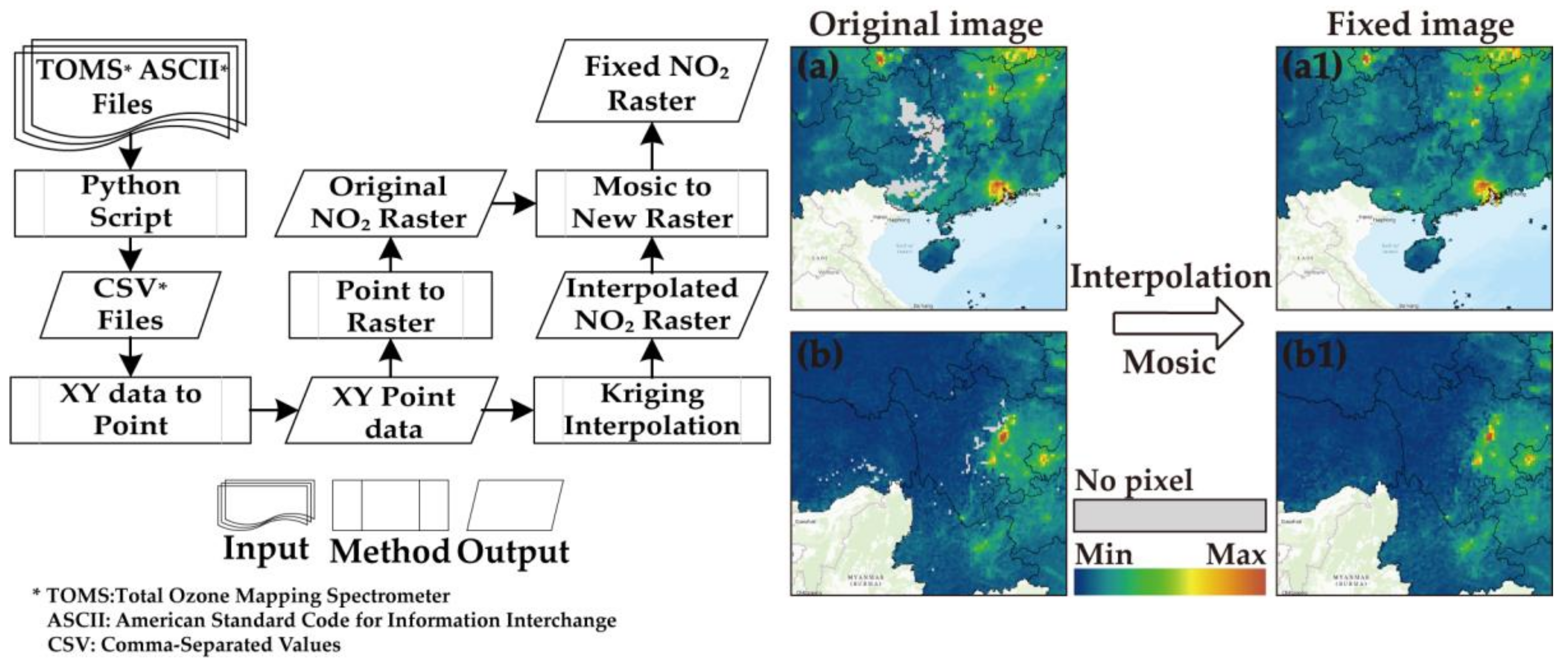
The tropospheric NO2 column concentration data used in this paper are produced by a TROPOMI instrument on a Sentinel-5 precursor (also known as Sentinel-5P). Sentinel-5P is the first Copernicus mission to monitor the atmosphere, with the aim of reducing the data gap between Envisat satellites (especially SCIAMACHY instruments) and the launch of Sentinel-5 [42]. The satellite carries the most advanced TROPOMI instrument for measuring ultraviolet-visible (270–500 nm), near-infrared (675–775 nm) and short-wave infrared (2305–2385 nm) spectral bands, which means it can image various air pollutants such as NO2, O3, CH2O, SO2, CH4, and CO more accurately than ever before [43]. Since Sentinel-5P Level-2 data products provide atmospheric geophysical parameters and the total column of trace gases, the monthly tropospheric NO2 column concentration data (February 2018–January 2019) from the Royal Netherlands Meteorological Research Institute (KNMI) are used in this paper. Following the technical route (Figure 2), the TOMS format files of tropospheric NO2 columns released by KNMI are rasterized to generate a time-series raster dataset. Besides, for the TROPOMI NO2 column products, a quality band ( ranging from 0 (poor) to 1 (excellent)) for performing pixel filtering is also provided to eliminate cloud interference and ensure data quality [38]. Since the research area of this paper is vast, and the weather changes significantly during the research period, the monthly NO2 columns used in this paper have the problem of pixel loss in some areas (). Therefore, based on the Kriging algorithm, the tropospheric NO2 column concentration in the pixel-loss region is interpolated (Figure 2).
The Suomi National Polar Orbiting Partnership (NPP), a near-polar geosynchronous orbit satellite with an orbital altitude of 824 km, carries a total of five sensors, and the Visible Infrared Imaging Radiometer Suite (VIIRS) is the most important of these [44]. VIIRS has 22 spectral bands with a spectral range of “0.3∼14 μm”. Among them, the Day/Night Band (DNB) operates in the visible and near-infrared spectrum, between 500 and 900 nm, to collect low-light imaging data. This paper uses the NPP/VIIRS DNB dataset to characterize surface dynamics in the analysis of the impact factor of NO2 columns in China. Specifically, we used the DNB images from February 2018 to January 2019 and eliminated the image background noise, based on the method proposed by Li et al. [45].
3.1.2. Statistical Bulletin Data
During the process of exploring the influencing factors of tropospheric NO2 column concentration, we also selected a series of socio-economic statistical indicators as potential impact factors, including population, GDP, industrial GDP and its proportion, social power consumption, total energy consumption, and motor vehicle ownership. These data (except for Hong Kong, Macao, and Taiwan) were mainly collected from national statistical databases, and provincial and prefectural Statistical Yearbooks of 2018. Moreover, the “China Urban Air Quality Monthly Report” published by the Ministry of Ecology and Environment of China was used to test coherence between NO2 tropospheric column concentration of Sentinel-5P and surface NO2 monitoring concentration [46]. The monthly report published the ranking of the average surface concentrations of major air pollutants in major cities in China, including the average surface concentrations of NO2 pollutants.
3.2. Spatial–Temporal Variation Models
Based on the preprocessed monthly NO2 tropospheric column concentration images of China, the spatial–temporal variation of NO2 tropospheric column concentration in provincial and prefectural administrative units was further explored. In this part, three models were applied to evaluate the spatial distribution characteristics of NO2 column concentration, aggregated by two kinds of administrative units, including coefficient of variation, and global and local spatial autocorrelation.
3.2.1. Coefficient of Variation of Tropospheric NO2 Columns
In statistics, the coefficient of variation (CV) is a normalized measure of the degree of dispersion of probability distribution [47]. Since CV can eliminate the influence of measurement scale and dimension when measuring data dispersion, it is widely used in geoscience and social statistics research [48]. CV is defined as the ratio of standard deviation to mean of data:
where represents the concentration of tropospheric NO2 column of administrative unit ; is the number of all administrative units; is the average tropospheric NO2 column concentration of all administrative units.
3.2.2. Spatial Autocorrelation of Troposphere NO2 Columns
As an important method in the study of spatial statistics, spatial autocorrelation reflects the spatial dependence between geographical attributes and adjacent units on a regional unit, including global spatial autocorrelation and local spatial autocorrelation [49]. As the most well known and widely used global spatial autocorrelation evaluation index, Global Moran’s I is usually used to describe the overall distribution of a geographical phenomenon or attribute value and to determine whether it has spatial aggregation characteristics [50]. The specific formula is as follows:
where represents the total number of administrative units; and represent the tropospheric NO2 column concentration of administrative unit and ; is the mean concentration of tropospheric NO2 column of all administrative units; and is the weight matrix of binary inverse distance space, which can be defined as the inverse of the distance among units and . At a given level of significance, the closer value approaches 1, the more significant the spatial aggregation of object attributes is; and the closer value approaches −1, the more significant the spatial divergence of object attributes is.
Unlike global spatial autocorrelation, local spatial autocorrelation is used to reflect the degree of correlation between a certain geographic phenomenon or attribute value on a local small-area unit and an adjacent local small-area unit [49]. To reveal the spatial heterogeneity of the tropospheric NO2 columns, we used the local spatial autocorrelation index Local Moran’s I to estimate the local autocorrelation [51]. The Local Moran’s I of spatial unit is defined as:
where is the variance of tropospheric NO2 column concentration. Under a specific level of significance, the administrative units can be divided into the following four categories on the basis of the results of Local Moran’s I: (a) High-High (HH) accumulation, where both administrative unit i and neighboring units have higher observations; (b) Low-Low (LL) aggregation, where both unit i and neighboring units have lower observations; (c) High-Low (HL) dispersion, where observations of adjacent units are lower than unit i; (d) Low-High (LH) dispersion, where observations of adjacent units are higher than unit i.
3.3. Impact Factors Analysis
3.3.1. Filtration of Impact Factors
As mentioned above, NO2 emissions in the troposphere are mainly man-made, mainly affected by population, urban economic development level, motor vehicle exhaust, and so on. Based on the references and prior knowledge, we collected statistical yearbooks and bulletins of various administrative units, and selected 10 socio-economic indicators including permanent population, GDP, secondary industry GDP and its proportion, tertiary industry GDP and its proportion, urbanization rate, whole society electricity consumption, total energy consumption, and vehicle ownership as potential NO2 column concentration impact factors. In addition, the light intensity mean and Digital Elevation Model (DEM) mean in each unit were extracted from NPP/VIIRS and SRTM3 Terrain Data to supplement the potential indicators. Parts of the indicators are explained as follows: (1) As anthropogenic emissions are the main source of tropospheric NO2, more people will probably bring more demand for emissions. (2) GDP is a key indicator of the economic situation of a country or region, while the secondary and tertiary industry GDP and its proportion can reflect the characteristics of China’s industrial structure. Previous studies have pointed out that industrial production is an important source of tropospheric NO2 emissions, so industrial restructuring will likely affect regional NO2 column concentrations. (3) Urbanization rate is the proportion of urban permanent residents in the region at the end of the year to the total resident population in the region, which is an indicator of the urbanization process. Therefore, the different levels of urbanization will cause differences in NO2 emissions. (4) Vehicle ownership is the stock of civil vehicles in the whole society of the region. Many literatures point out that automobile exhaust has become the main source of urban air pollution. (5) Nighttime light intensity is monitored by VIIRS sensor, which can effectively reflect the real vitality of the surface. Areas with high surface vitality tend to exchange more intense energy streams and produce more NO2 emissions. (6) For DEM, different terrain conditions (elevation) inevitably affect the intensity of human activity and the level of NO2 emissions [52]. Besides, since the economic statistics are published on an annual basis, the NO2 column concentration and monthly nighttime light data are synthesized annually in the impact factors analysis.
These potential impact factors and dependent variable (NO2 column concentration) may have multiple collinearities, so redundant variables need to be removed. Based on the spatial analysis module of ArcGIS, the Ordinary Least Square (OLS) was used to evaluate the degree of redundancy between variables, and the results showed that: (1) At the provincial units level, the Variance Inflation Factors (VIF) of population, GDP, secondary industry GDP, tertiary industry GDP, urbanization rate, total energy consumption, and vehicle ownership are greater than 7.5, indicating that there are obvious multiple collinearities among these variables [53]. Therefore, the indicators of nighttime light intensity, DEM, whole society electricity consumption, and the proportion of GDP in the secondary industry and tertiary industry are retained to evaluate the mechanisms of NO2 column concentration distribution in troposphere at the provincial unit scale. (2) At the prefectural unit level, especially the cities in the underdeveloped western regions, due to the serious incomplete records of socio-economic indicators, such as the whole society electricity consumption, total energy consumption, and the vehicle ownership, the Multicollinearity testing was performed only with a complete record. Finally, the indicators including the nighttime light intensity, DEM, population, and the proportion of secondary and tertiary industry GDP were selected to reveal the NO2 column concentration distribution mechanism at the prefecture unit level.
3.3.2. Spatial Econometric Model
Compared with the classical OLS linear model, the spatial economic model considers the spatial dependence effect of variables, which is the inheritance and development of traditional statistical methods. Generally, spatial economic models mainly include Spatial Lag Model (SLM) and Spatial Error Model (SEM) [54]. These two models are applicable to the spatial correlation of different spatial effects: 1) SLM is applied when there is significant spatial dependence between dependent variables; 2) SEM is applied when the error terms of the model are spatially correlated. The Lagrange multiplier test (LM) constructed by Burridge [55] and Anelin [52] is widely used in the selection of spatial econometric models because it can effectively detect the types of spatial effects. Hence, in this paper, Lagrange Multiplier (LM) test and Robust LM test are used to determine the appropriate spatial economic model for provincial units [56]. The results showed that LM-lag and Robust LM-lag have passed the significance test, while LM-Error and Robust LM-Error failed, so SLM was used to evaluate the impact factors of NO2 column concentration at the provincial unit level. The formula of the SLM model is as follows:
where is the vector of dependent variable (NO2 column concentration); is a data matrix of selected independent variables (impact factors, such as permanent population, GDP, etc.); is a vector of regression coefficient, which reflects the influence of independent variable on dependent variable ; is the spatial weight matrix, and is the coefficient of spatial lag variable ; is the random errors term.
3.3.3. Geographically Weighted Regression
The results of multiple collinear tests of prefectural administrative units show that the Koenker (BP) statistic of the model is significant, which means that the model has significant heteroscedasticity or instability in statistics. Regression models with statistically significant instability state are often well suited for performing Geographic Weighted Regression (GWR) analysis. The GWR Model Based on the first law of geography [57] extends the framework of the traditional OLS model, adds geographic location to regression parameters, and considers the spatial weights of adjacent points to allow local parameter estimation [58]. The calculation formula of the GWR model is as follows:
where is the dependent variable, the NO2 column concentration at point ; is the spatial coordinate of point ; is the regression coefficient of the independent variable k at point ; is the impact factors, and is the random errors terms.
4. Results
4.1. Coherence of NO2 Surface Concentration and Tropospheric Columns
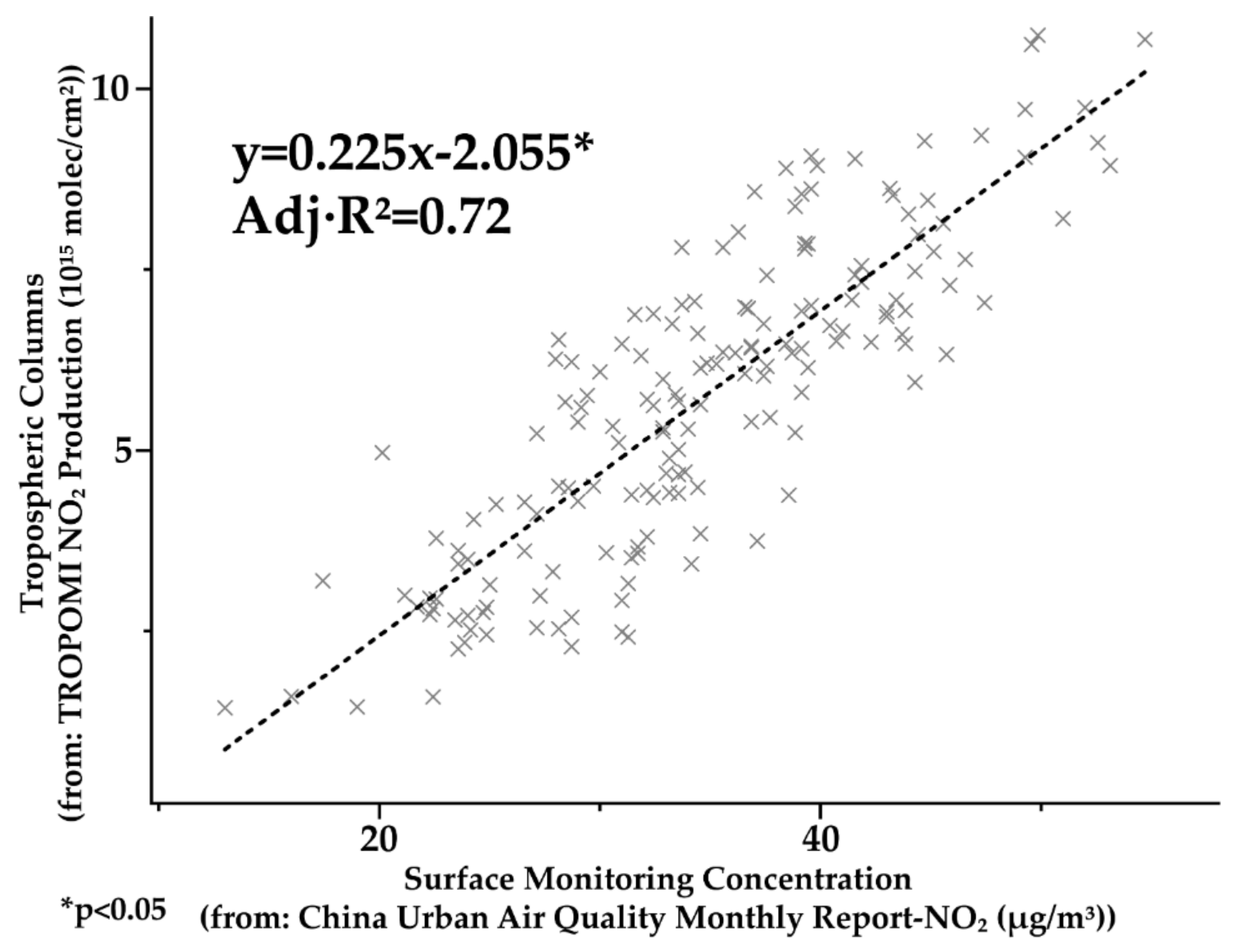
Until now, a series of ground experiments have shown that the NO2 column concentration based on remote sensing interpretation has a strong correlation with ground-based data, and the correlation coefficients are mostly above 0.8, which well reflects the characteristics of atmospheric NO2 concentration [59,60,61]. It is worth emphasizing that as the latest tropospheric NO2 column concentration inversion results, the coherence analysis of Sentinel-5P TROPOMI’s NO2 data and surface monitoring data is still insufficient, so it is useful to carry out a coherence analysis of NO2 surface monitoring concentration and tropospheric column concentration in China.
The China Urban Air Quality Monthly Report was used as the data source of NO2 surface monitoring concentration. The monthly report provides monthly averages of NO2 concentrations at surface monitoring stations in major cities in China (a total of 169 cities, accounting for 60% of all prefecture-level cities). In addition, on the basis of the monthly air quality report data, we selected multiperiod data (9 months available for public access) for mean processing, in order to reduce the interference of data occasional fluctuations and weather factors. The results of coherence analysis between NO2 monitoring concentration on urban surface and TROPOMI tropospheric column concentration are shown in Figure 3. The results show that the NO2 column concentration retrieved by TROPOMI is highly correlated with the surface monitoring concentration of NO2 on urban area (p < 0.05, Adj.R2 = 0.72).
4.2. Spatial–Temporal Characteristics of Tropospheric NO2 Columns
4.2.1. General characteristics
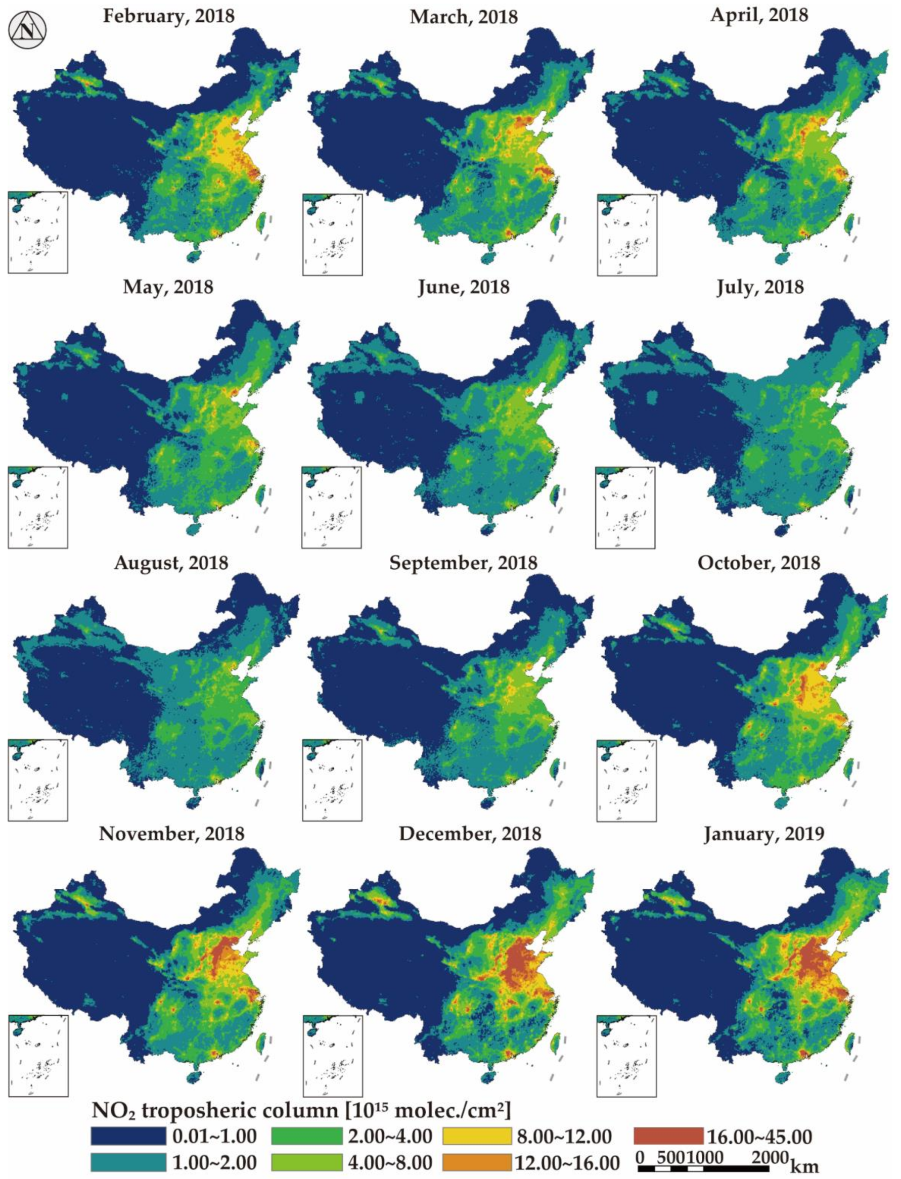
Figure 4 presents the monthly means maps of tropospheric NO2 columns from February 2018 to January 2019. The most significant feature of the tropospheric NO2 column concentration in China is that it is high in the east and low in the west. For western China, the NO2 column concentration in most areas is less than , while the areas with columns more than are mainly concentrated in Junggar Basin (Urumqi) and Turpan Basin (Turpan). For eastern China, the tropospheric NO2 column concentration above is mainly concentrated in the North China Plain (Hebei Province), Shandong Peninsula (Shandong Province), and the middle and middle-lower Yangtze Plain (Hubei, Anhui, Jiangsu Province, Shanghai). The North China Plain, with warm temperate monsoon climate, has insufficient precipitation and large seasonal variations in temperature. During winter, the decrease of temperature has greatly increased the demand for regional heating, and the consumption of coal has increased sharply. Besides, with abundant coal, iron, and petroleum deposits in the plain, the heavy industries such as coal, electricity, petroleum, chemical industry, and iron and steel occupy an important position in the region’s economic system. The special geographical conditions and socio-economic development background have led to the high concentration of tropospheric NO2 columns in the region, which has become the core of NO2 pollution areas in China. Another notable tropospheric NO2 column high-concentration agglomeration zone is the Middle-Lower Yangtze Plain, an important industrial base in China, with developed land and water transportation. Within the plain, there are two “peaks” of NO2 column concentration, which are the Yangtze River Delta Plain in the East and the Jianghan Plain in the west. The Yangtze River Delta Plain is one of the world’s famous estuary deltas. The advantageous geographical conditions have nurtured the Yangtze River Delta Urban Agglomeration (YRDUA), one of the six largest urban agglomerations in the world. As the most developed region in China, YRDUA is an important engine of China’s economic development, a 2.1% land area that concentrates 1/4 of the total economic output and industrial-added value of the whole country. The Jianghan Plain, located in the south-central part of Hubei Province, is one of the lowest elevations in China. The NO2 column concentration in Jianghan Plain shows a decreasing distribution from Wuhan City to the surrounding area. Wuhan is the capital of Hubei Province, the only sub-provincial city and mega-city in middle-China. As an important industrial base and core transportation hub in China, Wuhan has made remarkable achievements in urban construction and economic development in the recent ten years, but at the same time, it has also brought tremendous pressure to the environment and causes serious air pollution [62].
Besides, there are also several small-scale high-concentration NO2 distribution areas centered on the regional central cities. These small-scale NO2 column concentration distribution areas mainly include: Guangzhou and Shenzhen in South China, Chengdu and Chongqing in southwest China, Xi’an, Lanzhou, and Urumqi in western China, Anshan and Shenyang in northeast China. Most of the above cities are provincial capitals and regional central cities, where economic development level and human activity intensity are significantly higher than the local average level. The rapid development of economy and the increase of external population have increased NO2 anthropogenic emission sources, aggravated atmospheric pollution, and led to the sharp increase of NO2 column concentration in the troposphere around urban areas [63,64,65].
In this paper, the concentration data of tropospheric NO2 column from February 2018 to January 2019 were used for monthly statistics, and the results show that there was a significant seasonal variation of the tropospheric NO2 column concentration in China during the past year (Table 1). The minimum concentration of NO2 column in each month was relatively stable, with only slight fluctuation in June and August of 2018. The maximum of NO2 column concentration in each month had a significant difference, and the maximum value decreased from February 2018 to June 2018, and then rebounded to the highest level in January 2019. The monthly mean of NO2 column concentration was high in winter, low in summer, and transitional in spring and autumn, which is consistent with the observations of previous atmospheric monitoring satellites. Specifically, the mean concentration of NO2 in July and August of 2018 was the lowest (), while the mean value in December 2018 and January 2019 was the highest (about ).
At the national scale, the significant negative correlation between NO2 column concentration and temperature once again confirms that temperature is an important inducement for seasonal variation of NO2 column concentration. Except for the northwest China and Qinghai-Tibet Plateau, most of China is affected by the monsoon climate, with low temperature in winter and high temperature in summer. As a trace gas, the concentration of NO2 is determined not only by the total amount of emissions, but also by the intensity of solar radiation and other factors. Every winter, with the decrease of temperature, urban heating demand and coal consumption also increase rapidly, greatly increasing the NO2 emissions in the troposphere. Moreover, frequent cold, fog, snow, and frost weather in winter lead to weak solar radiation and a thick inversion layer in the troposphere, which is not conducive to the dissipation of NO2 and aggravates the concentration of NO2 column in the troposphere. Correspondingly, every summer, with the increase of solar radiation, rainwater, and the decrease of coal consumption, the decomposition of light and rainwater and the wet deposition will further reduce the concentration of pollutants in the atmosphere.
4.2.2. The Spatial Heterogeneity of NO2 Columns at Provincial Units
Figure 5 shows the monthly CV and Global Moran’s I of the tropospheric NO2 column concentration on the provincial units from February 2018 to January 2019. At the provincial unit level, the CV of NO2 column concentration fluctuated significantly, which indicated that there is a significant difference in the dispersion of the monthly tropospheric NO2 column concentration in China. Specifically, we found that the value of CV dropped rapidly from 0.9 in February to 0.56 in July, a drop of about 38%, and then increased month by month and returned to above 0.9 after November. In fact, the fluctuation characteristics of CV were similar to the mean fluctuation of NO2 column concentration, showing an obvious trend of “high in winter and low in summer”. The seasonal variations in NO2 emissions between different provinces are the possible causes of CV fluctuations. Although China has made remarkable achievements in social and economic development since its reform and development in 1978, the difference in regional development level has been further widened. The eastern coastal provinces benefit from the advantages of location and policy, and become the “first rich” area, while the inland provinces in the central and western regions, due to the limitations of natural conditions and other factors, make the region become the “second rich” area. Differences in economy, population, and urban development between eastern and western provinces will inevitably lead to differences in NO2 emissions. This difference will fluctuate regularly and periodically with the seasonal change. For example, during winter, the heating demand of eastern and northern provinces is significantly higher than that of southern and western provinces, which aggravates the emission of NO2 and other atmospheric pollutants, while in summer, the difference of NO2 emission between provinces decreases, and the NO2 column concentration CV of provincial units also drops to the lowest.
From the results of Global Moran’s I (p < 0.05), it clearly increased with a small fluctuation during the past year. Specifically, after the Global Moran’s I rose from 0.45 in February to 0.57, it fluctuated around 0.55 in the next few months, until September. Since October, the Global Moran’s I has increased significantly, and then reached its highest value in November, then fell back to about 0.65. Generally, the Global Moran’s I in autumn and winter is higher than that in spring and summer, which indicates that the aggregation distribution pattern of the tropospheric NO2 column concentration of the provincial units in the autumn and winter is more significant. In addition, we also found that the Global Moran’s I and CV fluctuations were synergistic for most of the time, except for June to July. In fact, CV measures the dispersion of data as a whole, while the Global Moran’s I measures the level of data aggregation after considering spatial location. Therefore, it can be considered that from May to July, although the dispersion degree of NO2 column concentration between provinces decreased, the aggregation degree of high and low values between provinces increased.
As shown by the results of local spatial autocorrelation (Figure 6), the four-month concentration data were used to explore Local Moran’s I change in different seasons. The results showed that in spring, the aggregation units of HH and LL in NO2 column concentration accounted for 95.0% of all significant units; in summer, the aggregation units accounted for 85.0% of all significant units; in autumn, the aggregation units of HH and LL accounted for 84.2% of all significant units; in winter, the aggregation units accounted for 86.4% of all significant units. The HH and LL aggregated units accounted for the majority of the significant units in the whole year, which indicated that the distribution of troposphere NO2 column concentration was mainly under the aggregation effect. From the spatial distribution HH and LL units, the LL aggregation was mainly distributed in western provinces including Qinghai, Tibet, Yunnan, Sichuan, Guangxi, and Guizhou, while the HH aggregation was concentrated in eastern provinces including Beijing, Hebei, Henan, Shandong, Shanxi, Anhui, Jiangsu, and Shanghai. Moreover, there were also provinces with low concentration of NO2 column such as Inner Mongolia, Hubei, Zhejiang, and so on around HH concentration provinces, which show as LH outlier.
4.2.3. The Spatial Heterogeneity of NO2 Columns at Prefectural Units
The CV fluctuations on prefectural units showed a typical “V” shape, that is, high in autumn, winter, and spring, but low in summer. Specifically, from February to July 2018, CV continued to decline from 0.85 to 0.52 (minimum), and then began to rise to 0.94 in January 2019 (Figure 5b). According to the fluctuation stage of CV, during the transition period from spring to summer, CV maintained a rapid decline of 38.8%, while in autumn and winter, CV continued to rise rapidly, with an increase of 80.8%. The variation of CV reflects that there are also significant differences in the dispersion degree of NO2 column concentration at prefectural units: during the summer, especially July and August, the difference of NO2 column concentration between cities is shrinking; in spring and autumn, the NO2 column concentration differences between cities is increasing, and reaches the maximum in winter. The periodic variation characteristics of the Global Moran’s I at prefectural units are similar to that of the provincial units, with only differences between February and March.
In addition, according to the Local Moran’s I of tropospheric NO2 column concentration in prefectural level, the units with spatial autocorrelation occupy the majority (Figure 7). The significant spatial autocorrelation units decreased from 283 in spring to 279 in summer, and then increased to 289 in autumn and 296 in winter. Besides, the proportion of HH and LL units in significant units in the four seasons also showed similar characteristics of “first falling then rising, high in winter and low in summer” (83.75%, 80.65%, 84.08%, and 85.47%). The high-value agglomeration units represented by HH mainly concentrated in eastern China, while the low-value agglomeration represented by LL mainly distributed in southwest and northeast China. The high-value discrete (high value surrounded by low value) units represented by HL are concentrated in Sichuan, China. The special topographic structure and development history of Sichuan Basin have resulted in a large number of people gathering, and a high concentration NO2 distribution area centered on Chengdu has been formed. Compared to the HL units, the number of low-value discrete units of LH is significantly more and mostly located in the transition zone between the LL aggregation and HH aggregation. In general, the spatial agglomeration of the tropospheric NO2 column concentration in the prefecture level has significant seasonal differences (high in winter and low in summer), and the distribution pattern of spatial agglomeration units is relatively stable.
4.3. Impact Factors of Tropospheric NO2 Columns
4.3.1. Impacts Factor Analysis at Provincial Units
Considering the availability of data, SLM was used to implement impact factors analysis, with NO2 column concentration in troposphere as dependent variable, nighttime light intensity, DEM, whole society electricity consumption, and the proportion of secondary and tertiary industries GDP as independent variables. The model performance indicators of R2, Log Likelihood, Akaike Info Criterion (AIC), and Schwarz Criterion are listed in Table 2, respectively. In this paper, the R2 and Log Likelihood of SLM were larger than OLS, while AIC and Schwarz Criterion were smaller than OLS. This showed that after consideration of the spatial effect, SLM effectively eliminates the spatial autocorrelation and improves the goodness of fit of the model, which is superior to the classical linear regression OLS model. Besides, according to the factor coefficients listed in Table 2, the nighttime light intensity, proportion of secondary and tertiary industries GDP are significant at provincial unit level. It is worth noting that the coefficients for the 3 factors are positive, which indicated that the human activity intensity and industrial structure can promote the regional concentration of NO2.
Actually, nighttime light intensity has been proved to be effective and accurate in reflecting the difference of human activity intensity and material energy distribution on the earth’s surface [66]. The regional higher nighttime light intensity means higher land development intensity and is usually accompanied by severe environmental pollution, especially for China, which is developing rapidly [67,68]. The regression coefficients of the secondary and tertiary industries GDP proportion reflect the contribution of industrial production, transportation, and services to regional NO2 column concentration.
4.3.2. Impact Factors Analysis at Prefectural Units
As mentioned above, through VIF and coefficient significance test in OLS model, we selected the independent variables from the ensemble of available variables, including nighttime light intensity, DEM, population, and the proportion secondary and tertiary industries GDP. Since bandwidth is a key parameter in GWR, the AIC method was used to determine the most bandwidth to ensure the fit and smoothness of the model. The model performance evaluation indicators of the GWR and OLS at the prefecture level (Table 3) showed that the R2 rises from 0.505 for OLS to 0.643 for GWR, and AICc (corrected AIC) also drops from 1488 to 1395, which indicates that the performance of the GWR model with local parameter estimation is better than OLS.
Meanwhile, we made statistics on the independent variable coefficients of prefecture units. The results showed that among the selected independent variables, the coefficients of nighttime light intensity, the proportion of secondary and tertiary industries, and the population were positive, which indicated that these factors have a positive correlation with the NO2 column concentration; the coefficient of DEM was negative, which means that the higher the terrain, the lower the concentration of NO2. Unlike OLS, GWR model provides local model results for predicted variables and gives Adj.R2 and each independent variable coefficient for each prefectural unit. Although the entirety R2 of GWR reached 0.643, there were still significant differences in R2 of each prefecture unit. As shown in Figure 8, the Local R2 increased gradually from east to west, and the independent variables of the eastern coastal cities can only explain about 50% of the dependent variables, while the model explanatory power of the western inland cities can reach more than 75%.
Similarly, the coefficients of the independent variables between regions are also differences. For example, the coefficient of nighttime light intensity increased from southeast to northwest, indicating that the effect of light intensity on NO2 column concentration increases from southeast to northwest (Figure 8). The reason for this phenomenon may be the difference of regional economic development level. The southeast of China is the most economically developed and populous region in China due to geographical conditions, policy conditions, and historical development, while the northwest of China is less developed due to the restrictions of natural conditions and transportation. Compared with the northwestern region, the nighttime light intensity between cities in southeastern China was relatively close, which cannot effectively reveal the difference in nitrogen dioxide concentration in the region.
5. Discussion
5.1. Division Line of Tropospheric NO2 Columns
Generally, the areas with high NO2 column concentration are located in the southeast of China, while the low value areas are mostly located in the Northwest inland. By extracting the high and low boundary lines of NO2 column concentration, we generated a NO2 column concentration division line (Figure 9). This division line is mainly composed of a series of mountains, including Lesser Khingan, Great Khingan, Yin Mountains, Helan Mountains, Qilian Mountains, Laji Mountains, Min Mountains, and Hengduan Mountains. To a certain extent, the division line, which consists of the series of mountains, restricts the westward diffusion of NO2 in the eastern developed areas and gradually forms the spatial distribution pattern of NO2 column concentration in China, which is an east-high and west-low pattern.
It is worth noting that the NO2 column concentration division line is quite similar to the Hu Line. Hu Line, also known as Heihe−Tengchong Line, was proposed in 1935 by Hu Huanyong, a Chinese geographer [69]. In addition, the Hu Line coincides with the 400 mL precipitation line and the demarcation line between monsoon and non-monsoon climate. This line has even become the dividing line of China’s urbanization level. Most cities on the southeast side of the line have higher urbanization levels than the national average, while the cities on the northwest side of the line are usually lower than the average. The differences in natural geographical conditions, economic development levels, and population aggregation on both sides of the Hu Line led to significant differences in tropospheric NO2 emissions and gradually shaped the NO2 column concentration distribution pattern in China. Therefore, in order to simplify the division line, we can roughly assume that Hu Line is not only the boundary line between population density and urbanization level, but also the division line of tropospheric NO2 column concentration in China. It must be emphasized that this is the first report on a similar dividing line between the Hu line and the NO2 column concentration.
5.2. Spatial−Temporal Characteristics Comparison at Different Administrative Units Level
The comparison of CV fluctuations between provincial and prefectural units from February 2018 to January 2019 showed a similar fluctuation evolution. For both administrative units levels, the highest CV in winter was around 0.9; the lowest CV in summer was between 0.5 and 0.6; the spring (autumn) season is the transition period of CV and showed a trend of decreasing (increasing) month by month. Although the seasonal fluctuation trend of CV between the levels was similar, there were still some differences in the fluctuation of CV during winter. As can be seen from Figure 10a, during the winter (Nov 2018–Jan 2019), the CV of the provincial units showed slight fluctuations around 0.9, while the CV of the prefecture-level units maintained a relatively stable growth. We believe that there are two main reasons for this difference: on the one hand, there are 34 provincial units in China, while 333 prefectural administrative units. Provincial units with less NO2 column concentration samples increase the instability and discreteness of data, resulting in higher CV. On the other hand, provincial units are composed of several prefectural units, which will lead the provincial units to “amplify” or “narrow” the range of NO2 change of prefectural units in the region, resulting in prominent differences between provincial units.
Unlike the high similarity of fluctuation trend between two levels of CV, the fluctuation of Global Moran’s I appears significant differences at different levels of administrative units. First, the provincial-level Global Moran’s I was higher than the prefectural-level units; second, there were inconsistencies in the direction of data fluctuations in some months. For example, from February to March, the Global Moran’s I showed an upward trend in provincial units and a downward trend in prefectural units; from October to December, the Global Moran’s I of provincial units rose first and then decreased, while the Global Moran’s I of prefectural units showed the opposite trend. We speculate that the main reason for this difference is the “delayed effect” caused by different observational scales in the process of concentration and dispersion of NO2. From February to March, the NO2 emission decreased as the temperature rose, and the column concentration of tropospheric NO2 decreased accordingly. The reduction of NO2 column concentration is more obvious in cities with high NO2 concentration, which leads to the reduction of high value agglomeration and the decrease of Global Moran’s I. For provincial units, the larger space scales with multiple prefecture-level cities serve as a “buffer” when NO2 begins to decline, which delays the change of the Global Moran’s I caused by the change of NO2 column concentration. From September to November, with the decrease of temperature, the NO2 emission of prefecture-level cities increased, the NO2 column concentration in the troposphere increased, and the Global Moran’s I of prefectural units rose rapidly. Similarly, the rise of the Global Moran’s I was delayed due to the delayed effect at the provincial level. In Figure 10b, the fluctuation trend of the adjusted Global Moran’s I of prefecture-level cities is highly similar to that of the provincial-level Global Moran’s I, which further confirms that the provincial units with a larger spatial range have a one-month “delayed effect” of the fluctuation.
From the analysis of Local Moran’s I, it can be seen that the distribution of HH agglomeration units in provincial and prefectural units is similar, that is, HH agglomeration is mainly concentrated in North China Plain and the middle-lower Yangtze Plain. For LL agglomeration, the LL agglomeration units number of prefectural level has been expanded compared with provincial level, and LL agglomeration have also appeared in northeast China. In addition, another noteworthy difference is HL distribution. The NO2 column concentration of provincial units is the average value of the cities under the jurisdiction, thus ignoring the discrete situation within provincial units. Conversely, because of the small spatial scale of prefectural units, there are also differences in NO2 column concentration between cities in the province, which affects the evaluation level of high-value aggregation and low-value aggregation.
5.3. The Impact Factors Analysis at Different Administrator Units Level
By comparing the impact factors at different administrative levels, we can find that the light intensity and the proportion of secondary and tertiary industries are always the positive factors affecting the distribution of NO2 column concentration, while DEM is the negative factor. The difference is that population also plays a positive role in promoting the distribution of NO2 column concentration in prefecture-level cities. In fact, the CV of population and NO2 column concentration in provincial units are quite different (Population: 0.45; NO2: 0.812), while those in prefectural units are relatively close (Population: 0.86; NO2: 0.77). This indicates that the discrete degree of population and NO2 column concentration at the prefectural level is closer compare with provincial units, so it can be selected as an effective independent variable to participate in the regression model.
Besides, the goodness of fit of GWR model with local regression at prefectural level is higher than SLM model in provincial units. With the reduction of spatial scale of spatial evaluation units and the increase of the number of units, the difference of NO2 column concentration between cities is highlighted. In the case of the statistically significant unsteady regression model, the GWR model based on local regression can restore the local characteristics of variables and better fit the distribution of NO2 column concentration than the provincial SLM model.
Although GWR performs well in overall fitting performance, the significant aggregation of standardized residuals reflects the absence of key variables in high concentration NO2 agglomeration areas, especially in North China and East China (Figure 11). Therefore, we re-executed GWR modeling in cities with higher than 1.5 times standardized residuals in North and East China. For East China and North China, due to the close relationship and social-economic development between cities, the statistical data is more robust than the western cities. Hence, in the sub-region, the whole society electricity consumption and vehicle ownership are supplemented as new independent variables to participate in the construction of the model. The results showed that the Adj.R2 of the new model with independent variables reaches 0.685 (previous model: 0.620), and the distribution of the standardized residuals of the new model presents random distribution (Global Moran’s I = 0.04, p < 0.05). At present, many scholars have shown that with the rapid increase in the number of urban motor vehicles and the rising energy consumption, the proportion of NO2 from coal-fired emissions and motor vehicle exhaust in tropospheric NO2 is also increasing, and the problem of NO2 pollution is more serious than ever [70,71,72]. Moreover, due to the flat terrain and the leading economic level between cities in North China and East China, the NO2 pollutants in the region transfer and influence each other among cities, forming a huge “North China−East China NO2 pollution system”.
6. Conclusions
Based on the NO2 data products of Sentinel-5P with TROPOMI, the spatial−temporal characteristics and impact factors of tropospheric NO2 column concentration in China in 2018 were analyzed at provincial and prefectural levels in this paper. It is an application of NO2 data products based on the Sentinel-5P TROPOMI sensor in China. The results of the study clarify the seasonal effect and agglomeration effect of the NO2 column concentration distribution in China, which could help us better understand the distribution pattern of tropospheric NO2 pollutants in China and its potential impact factors. The coherence analysis with the NO2 surface monitoring concentration released by China Urban Air Quality Monthly Report reflects the high correlation between the NO2 column concentration inverted by TROPOMI and the measured surface concentration, which reveals the great potential of the TROPOMI NO2 column concentration in indicating urban surface air pollution conditions. The analysis of the spatial−temporal characteristics of the tropospheric NO2 column concentration shows that: (1) the monthly fluctuation of the tropospheric NO2 column concentration has a significant “winter high summer low” cycle characteristic; (2) the spatial distribution pattern of NO2 column concentration in troposphere shows a general pattern of “east-high and west-low”, and the division line between the eastern high-value area and the western low-value area of NO2 column concentration is close to the Hu Line; (3) the results of CV and spatial autocorrelation models at two kinds of administrative scales show that although the spatial heterogeneity of NO2 column concentration does not differ significantly with the scale change, NO2 column concentration has a certain degree of “delayed effect” during the fluctuation process. Furthermore, the results of modelling and impact factors analysis of NO2 column concentration at different levels show that: (4) nighttime light intensity, the proportion of secondary and tertiary industries GDP, and tropospheric NO2 column concentration are positively correlated at two administrative levels; while population is positively correlated with NO2 only at the prefecture level; (5) within the areas with high concentration of NO2 pollution in North China and East China, the whole social electricity consumption and vehicle ownership also play a positive role in promoting the column concentration of NO2.
The results of the present study have implications for governments and policymakers to develop effective NO2 emissions reduction and air pollution prevention policies. Firstly, the tropospheric NO2 pollution in China has serious spatial differences, which requires us to adopt “local measures” to deal with NO2 pollution. Among them, North China and East China, as the most serious and concentrated areas of NO2 pollution in China, should take measures to optimize industrial integration and limit the number and total emissions of enterprises with high pollution and energy consumption. Meanwhile, the government should urge enterprises to increase investment in research and development of emission reduction technology to minimize the direct emission of NO2 pollutants. For the underdeveloped areas in Western China, the column concentration of NO2 is still in a low state, and the overall pollution situation can be neglected. Therefore, for the western region, the government should also take economic development as its main goal while controlling NO2 emissions. Furthermore, considering the seasonal variation of NO2 pollution, it is necessary and effective to adjust the NO2 emission strategy seasonally.
Although the spatial−temporal characteristics and impact factors of NO2 column concentration distribution in China are analyzed, there are still some limitations and shortcomings in this paper. For example, the incompleteness and partial absence of socio-economic statistics in prefectural units greatly limit the analysis of influential factors of NO2 pollution. Therefore, the next stage of research should focus on exploring the impact mechanism of NO2 pollutants at the local scale to guide the formulation of fine-scale NO2 pollution control policies. Besides, since Sentinel-5P’s NO2 data monthly products are only available after February 2018, the longer time-scale fluctuation studies, such as the annual variation of NO2 column concentration in China, cannot be implemented. As TROPOMI atmospheric monitoring data is being produced continuously, the available datasets are expanding. Therefore, collecting dynamically updated NO2 column concentration data and carrying out long-span fluctuation analysis of air pollutants will also be our next focus.
Author Contributions
Conceptualization, Z.Z. and F.M.; Funding acquisition, Z.W. and F.M.; Methodology, Z.Z.; Project administration, Z.W.; Software, Z.Z. and Z.Y.; Supervision, Z.W. and F.M.; Validation, Z.Z. and Z.Y.; Writing–original draft, Z.Z.; Writing–review & editing, F.M.
Funding
This study has been supported by National Social Science Foundation of China (41671430) and Natural Science Foundation of Guangdong Province (2018B030312004).
Acknowledgments
We acknowledge the free use of tropospheric NO2 column data from the TROPOMI (Sentinel-5P) sensor from www.temis.nl. We also want to express our sincere gratitude to the anonymous reviews and editors for their efforts in the improvement of the paper.
Conflicts of Interest
The authors declare no conflict of interest.
References
- Guan, X.L.; Wei, H.K.; Lu, S.S.; Dai, Q.; Su, H.J. Assessment on the urbanization strategy in China: Achievements, challenges and reflections. Habitat Int. 2018, 71, 97–109. [Google Scholar] [CrossRef]
- Richter, A.; Burrows, J.P.; Nüß, H.; Granier, C.; Niemeier, U. Increase in tropospheric nitrogen dioxide over China observed from space. Nature 2005, 437, 129. [Google Scholar] [CrossRef] [PubMed]
- Van Der A, R.J.; Peters, D.H.M.U.; Eskes, H.; Boersma, K.F.; Van Roozendael, M.; De Smedt, I.; Kelder, H.M. Detection of the trend and seasonal variation in tropospheric NO2 over China. J. Geophys. Res. Atmos. 2006, 111. [Google Scholar] [CrossRef]
- Duncan, B.N.; Lamsal, L.N.; Thompson, A.M.; Yoshida, Y.; Lu, Z.F.; Streets, D.G.; Hurwitz, M.M.; Pickering, K.E. A Space-based, high-resolution view of notable changes in urban NOX pollution around the world (2005–2014). J. Geophys. Res. Atmos. 2016, 121, 976–996. [Google Scholar] [CrossRef]
- Schneider, P.; Lahoz, W.A.; Van der, A.R. Recent satellite-based trends of tropospheric nitrogen dioxide over large urban agglomerations worldwide. Atmos. Chem. Phys. 2015, 15, 1205–1220. [Google Scholar] [CrossRef] [Green Version]
- Georgoulias, A.K.; Van der A, R.J.; Stammes, P.; Boersma, K.F.; Eskes, H.J. Trends and trend reversal detection in 2 decades of tropospheric NO2 satellite observations. Atmos. Chem. Phys. 2019, 19, 6269–6294. [Google Scholar] [CrossRef]
- Seinfeld, J.H.; Pandis, S.N.; Noone, K. Atmospheric chemistry and physics: From air pollution to climate change. Phys. Today 1998, 51, 88. [Google Scholar] [CrossRef]
- Crutzen, P.J. The role of NO and NO2 in the chemistry of the troposphere and stratosphere. Annu. Rev. Earth Planet. Sci. 1979, 7, 443–472. [Google Scholar] [CrossRef]
- Crutzen, P.J.; Schmailzl, U. Chemical budgets of the stratosphere. Planet. Space Sci. 1983, 31, 1009–1032. [Google Scholar] [CrossRef]
- Lee, D.S.; Köhler, I.; Grobler, E.; Rohrer, F.; Sausen, R.; Gallardo-Klenner, L.; Olivier, J.G.; Dentener, F.J.; Bouwman, A.F. Estimations of global no, emissions and their uncertainties. Atmos. Environ. 1997, 31, 1735–1749. [Google Scholar] [CrossRef]
- Solomon, S.; Qin, D.; Manning, M.; Chen, Z.; Marquis, M.; Averyt, K.; Tignor, M.; Miller, K.L. The physical science basis. In Contribution of Working Group I to the Fourth Assessment Report of the Intergovernmental Panel on Climate Change; Cambridge University Press: Cambridge, UK; New York, NY, USA, 2007. [Google Scholar]
- Beirle, S.; Platt, U.; Wenig, M.; Wagner, T. Weekly cycle of NO2 by GOME measurements: A signature of anthropogenic sources. Atmos. Chem. Phys. 2003, 3, 2225–2232. [Google Scholar] [CrossRef]
- Van Der A, R.J.; Eskes, H.J.; Boersma, K.F.; Van Noije, T.P.C.; Van Roozendael, M.; De Smedt, I.; Peters, D.H.M.; Meijer, E.W. Trends, seasonal variability and dominant NOX source derived from a ten year record of NO2 measured from space. J. Geophys. Res. Atmos. 2008, 113. [Google Scholar] [CrossRef]
- Tian, H.; Wang, Y.; Zhao, D.; Chai, F.; Xing, Z.; Chen, K. Zhongguo Taihangshan Donglu NOX Zhongwuran Chengyin Fenxi. Chin. Sci. Bull. 2011, 56, 1464–1469. [Google Scholar]
- Huang, H.J.; Fu, D.Y.; Qi, W. Effect of driving restrictions on air quality in Lanzhou, China: Analysis integrated with internet data source. J. Clean. Prod. 2017, 142, 1013–1020. [Google Scholar] [CrossRef]
- Diao, B.D.; Zeng, K.F.; Su, P.D.; Ding, L.; Liu, C. Temporal-spatial distribution characteristics of provincial industrial NOX emissions and driving factors in China from 2006 to 2013. Resour. Sci. 2016, 38, 1768–1779. [Google Scholar]
- Hendrick, F.; Mahieu, E.; Bodeker, G.E.; Boersma, K.F.; Chipperfield, M.P.; Maziere, M.D.; Smedt, I.D.; Demoulin, P.; Fayt, C.; Hermans, C.; et al. Analysis of stratospheric NO2 trends above Jungfraujoch using ground-based UV-visible, FTIR, and satellite nadir observations. Atmos. Chem. Phys. 2012, 12, 8851–8864. [Google Scholar] [CrossRef]
- Velders, G.J.; Granier, C.; Portmann, R.W.; Pfeilsticker, K.; Wenig, M.; Wagner, T.; Platt, U.; Richter, A.; Burrows, J.P. Global tropospheric NO2 column distributions: Comparing three-dimensional model calculations with GOME measurements. J. Geophys. Res. Atmos. 2001, 106, 12643–12660. [Google Scholar] [CrossRef]
- Zhang, X.; Zhang, P.; Zhang, Y.; Li, Y.; Qiu, H. Zhongguo Duiliuceng NO2 de Bianhua Qushi, Shikong Fenbu Tezheng Jiqi Laiyuan Jiexi. Sci. China 2007, 37, 1409. [Google Scholar]
- Xiao, Z.; Jiang, H.; Chen, M. Characteristics of atmospheric NO2 over China using OMI remote sensing data. Acta Sci. Circumstantiae 2011, 31, 2080–2090. [Google Scholar]
- Sun, C.W.; Luo, Y.; Li, J.L. Urban traffic infrastructure investment and air pollution: Evidence from the 83 cities in China. J. Clean. Prod. 2018, 172, 488–496. [Google Scholar] [CrossRef]
- Liu, W.Q.; Chen, Z.Y.; Liu, J.G.; Xie, P.H. Stereoscopic monitoring technology and applications for the atmospheric environment in China. Chin. Sci. Bull. 2016, 61, 3196–3207. [Google Scholar] [CrossRef] [Green Version]
- Tømmervik, H.; Johansen, B.E.; Pedersen, J.P. Monitoring the effects of air pollution on terrestrial ecosystems in Varanger (Norway) and Nikel-Pechenga (Russia) using remote sensing. Sci. Total Environ. 1995, 160, 753–767. [Google Scholar] [CrossRef]
- Emeis, S.; Schäfer, K. Remote sensing methods to investigate boundary-layer structures relevant to air pollution in cities. Bound. Layer Meteorol. 2006, 121, 377–385. [Google Scholar] [CrossRef]
- Gupta, P.; Christopher, S.A.; Wang, J.; Gehrig, R.; Lee, Y.C.; Kumar, N. Satellite remote sensing of particulate matter and air quality assessment over global cities. Atmos. Environ. 2006, 40, 5880–5892. [Google Scholar] [CrossRef]
- Peng, J.; Chen, S.; Lv, H.L.; Liu, Y.X.; Wu, J.S. Spatiotemporal patterns of remotely sensed PM2.5 concentration in China from 1999 to 2011. Remote Sens. Environ. 2016, 174, 109–121. [Google Scholar] [CrossRef]
- Xue, T.; Zheng, Y.X.; Geng, G.N.; Zheng, B.; Jiang, X.J.; Zhang, Q.; He, K.B. Fusing observational, satellite remote sensing and air quality model simulated data to estimate spatiotemporal variations of PM2.5 exposure in China. Remote Sens. 2017, 9, 221. [Google Scholar] [CrossRef]
- Marinello, F. Last generation instrument for agriculture multispectral data collection. Agric. Eng. Int. CIGR J. 2017, 19, 87–93. [Google Scholar]
- Stolarski, R.S.; Bloomfield, P.; McPeters, R.D.; Herman, J.R. Total ozone trends deduced from Nimbus 7 TOMS data. Geophys. Res. Lett. 1991, 18, 1015–1018. [Google Scholar] [CrossRef]
- Burrows, J.P.; Weber, M.; Buchwitz, M.; Rozanov, V.; Ladstätter-Weißenmayer, A.; Richter, A.; DeBeek, R.; Hoogen, R.; Bramstedt, K.; Eichmann, K.; et al. The global ozone monitoring experiment (GOME): Mission concept and first scientific results. J. Atmos. Sci. 1999, 56, 151–175. [Google Scholar] [CrossRef]
- Desnos, Y.L.; Buck, C.; Guijarro, J.; Levrini, G.; Suchail, J.L.; Torres, R.; Laur, H.; Closa, J.; Rosich, B. The ENVISAT advanced synthetic aperture radar system. In Proceedings of the IGARSS 2000. IEEE 2000 International Geoscience and Remote Sensing Symposium, Honolulu, HI, USA, 24–28 July 2000; Volume 3, pp. 1171–1173. [Google Scholar]
- Krotkov, N.A.; McLinden, C.A.; Li, C.; Lamsal, L.N.; Celarier, E.A.; Marchenko, S.V.; Swartz, W.H.; Bucsela, E.J.; Joiner, J.; Duncan, B.N.; et al. Aura OMI observations of regional SO2 and NO2 pollution changes from 2005 to 2015. Atmos. Chem. Phys. 2016, 16, 4605–4629. [Google Scholar] [CrossRef]
- Munro, R.; Lang, R.; Klaes, D.; Poli, G.; Retscher, C.; Lindstrot, R.; Huckle, R.; Lacan, A.; Grzegorski, M.; Holdak, A.; et al. The GOME-2 instrument on the Metop series of satellites: Instrument design, calibration, and level 1 data processing-An overview. Atmos. Meas. Tech. 2016, 9, 1279–1301. [Google Scholar] [CrossRef]
- Hassinen, S.; Balis, D.; Bauer, H.; Begoin, M.; Delcloo, A.; Eleftheratos, K.; Garcia, S.G.; Granville, J.; Grossi, M.; Hao, N.; et al. Overview of the O3M SAF GOME-2 operational atmospheric composition and UV radiation data products and data availability. Atmos. Meas. Tech. 2016, 9, 383–407. [Google Scholar] [CrossRef] [Green Version]
- Showstack, R. Sentinel satellites initiate new era in earth observation. Eos Trans. Am. Geophys. Union 2014, 95, 239–240. [Google Scholar] [CrossRef]
- Berger, M.; Moreno, J.; Johannessen, J.A.; Levelt, P.F.; Hanssen, R.F. ESA’s sentinel missions in support of Earth system science. Remote Sens. Environ. 2012, 120, 84–90. [Google Scholar] [CrossRef]
- Guanter, L.; Aben, I.; Tol, P.; Krijger, J.M.; Hollstein, A.; Köhler, P.; Damm, A.; Joiner, J.; Frankenberg, C.; Landgraf, J. Potential of the TROPOspheric Monitoring Instrument (TROPOMI) onboard the Sentinel-5 Precursor for the monitoring of terrestrial chlorophyll fluorescence. Atmos. Meas. Tech. 2015, 8, 1337–1352. [Google Scholar] [CrossRef] [Green Version]
- S5P Mission Performance Centre Nitrogen Dioxide [L2 NO2] Readme. Available online: https://sentinel.esa.int/documents/247904/3541451/Sentinel-5P-Nitrogen-Dioxide-Level-2-Product-Readme-File (accessed on 23 July 2019).
- Guan, D.; Hubacek, K.; Weber, C.L.; Peters, G.P.; Reiner, D.M. The drivers of Chinese CO2 emissions from 1980 to 2030. Glob. Environ. Chang. 2008, 18, 626–634. [Google Scholar] [CrossRef]
- Li, K.; Bai, K.X. Spatiotemporal associations between PM2.5 and SO2 as well as NO2 in China from 2015 to 2018. Int. J. Environ. Res. Public Health 2019, 16, 2352. [Google Scholar] [CrossRef]
- Li, Y.; Wei, Y.D. The spatial-temporal hierarchy of regional inequality of China. Appl. Geogr. 2010, 30, 303–316. [Google Scholar] [CrossRef]
- Veefkind, J.P.; Aben, I.; McMullan, K.; Förster, H.; De Vries, J.; Otter, G.; Class, J.; Eskes, H.J.; De Haan, J.F.; Kleipool, Q.; et al. TROPOMI on the ESA Sentinel-5 Precursor: A GMES mission for global observations of the atmospheric composition for climate, air quality and ozone layer applications. Remote Sens. Environ. 2012, 120, 70–83. [Google Scholar] [CrossRef]
- Galli, A.; Butz, A.; Scheepmaker, R.A.; Hasekamp, O.; Landgraf, J.; Tol, P.; Wunch, D.; Deutscher, P.O.; Toon, G.C.; Wennberg, P.O.; et al. CH4, CO, and H2O spectroscopy for the Sentinel-5 Precursor mission: An assessment with the Total Carbon Column Observing Network measurements. Atmos. Meas. Tech. 2012, 5, 1387–1398. [Google Scholar] [CrossRef]
- Cao, C.; Xiong, J.; Blonski, S.; Liu, Q.; Uprety, S.; Shao, X.; Bai, Y.; Weng, F. Suomi NPP VIIRS sensor data record verification, validation, and long-term performance monitoring. J. Geophys. Res. Atmos. 2013, 118, 11–664. [Google Scholar] [CrossRef]
- Li, F.; Wei, A.H.; Mi, X.N.; Sun, G.T. An approach of GDP spatialization in Hebei Province using NPP/VIIRS nighttime light data. J. Xinyang Norm. Univ. 2016, 29, 152–156. [Google Scholar]
- Monthly Report on Urban Air Quality. Available online: http://www.mee.gov.cn/hjzl/dqhj/cskqzlzkyb/ (accessed on 23 July 2019).
- Abdi, H. Coefficient of variation. Encycl. Res. Des. 2010, 1, 169–171. [Google Scholar]
- Reed, G.F.; Lynn, F.; Meade, B.D. Use of coefficient of variation in assessing variability of quantitative assays. Clin. Vaccine Immunol. 2002, 9, 1235–1239. [Google Scholar] [CrossRef] [PubMed]
- Zhang, J.Q.; Chen, J.F. Study on construction land distribution in Fujian and Taiwan Provinces based on spatial autocorrelation analysis. Prog. Geogr. 2007, 26, 11–17. [Google Scholar]
- Boots, B.; Tiefelsdorf, M. Global and local spatial autocorrelation in bounded regular tessellations. J. Geogr. Syst. 2000, 2, 319–348. [Google Scholar] [CrossRef]
- Premo, L.S. Local spatial autocorrelation statistics quantify multi-scale patterns in distributional data: An example from the Maya Lowlands. J. Archaeol. Sci. 2004, 31, 855–866. [Google Scholar] [CrossRef]
- Yang, W.; Chen, B.Y.; Cao, X.; Li, T.; Li, P. The spatial characteristics and influencing factors of modal accessibility gaps: A case study for Guangzhou, China. J. Transp. Geogr. 2017, 60, 21–32. [Google Scholar] [CrossRef]
- Burridge, P. On the Cliff-Ord Test for Spatial Correlation. J. R. Stat. Soc. 1980, 42, 107–108. [Google Scholar] [CrossRef]
- Anselin, L. Lagrange Multiplier Test Diagnostics for Spatial Dependence and Spatial Heterogeneity. Geogr. Anal. 1988, 20, 1–17. [Google Scholar] [CrossRef]
- Wang, P.; Wu, W.; Zhu, B.; Wei, Y. Examining the impact factors of energy-related CO2 emissions using the STIRPAT model in Guangdong Province, China. Appl. Energy 2013, 106, 65–71. [Google Scholar] [CrossRef]
- Xie, X.; Liao, L. A study on the relationship between tourism development and economic growth in Yunnan Province based on spatial econometric model. J. Kunming Univ. Sci. Technol. 2015, 15, 77–84. [Google Scholar]
- Tobler, W. On the first law of geography: A reply. Ann. Assoc. Am. Geogr. 2004, 94, 304–310. [Google Scholar] [CrossRef]
- Wheeler, D.C.; Calder, C.A. An assessment of coefficient accuracy in linear regression models with spatially varying coefficients. J. Geogr. Syst. 2007, 9, 145–166. [Google Scholar] [CrossRef]
- Kramer, L.J.; Leigh, R.J.; Remedios, J.J.; Monks, P.S. Comparison of OMI and ground-based in situ and MAX-DOAS measurements of tropospheric nitrogen dioxide in an urban area. J. Geophys. Res. Atmos. 2008, 113. [Google Scholar] [CrossRef]
- Bucsela, E.J.; Perring, A.E.; Cohen, R.C.; Boersma, K.F.; Celarier, E.A.; Gleason, J.F.; Wenig, M.O.; Bertram, T.H.; Wooldridge, P.J.; Dirksen, R.; et al. Comparison of tropospheric NO2 from in situ aircraft measurements with near-real-time and standard product data from OMI. J. Geophys. Res. Atmos 2008, 113. [Google Scholar] [CrossRef]
- Huijnen, V.; Eskes, H.J.; Poupkou, A.; Elbern, H.; Boersma, K.F.; Foret, G.; Sofiev, M.; Valdebenito, A.; Flemming, J.; Stein, O.; et al. Comparison of OMI NO2 tropospheric columns with an ensemble of global and European regional air quality models. Atmos. Chem. Phys. 2010, 10, 3273–3296. [Google Scholar] [CrossRef]
- Qiu, P.; Tang, X.; Lu, M.; Huang, Y.; Zhou, J. Forecast of changing air pollution trends in Wuhan city. J. Nanjing Univ. Inf. Sci. Technol. 2018, 10, 571–578. [Google Scholar]
- Ma, W.; Li, Y.H.; Hou, X.G. Characteristics of Atmospheric NO2 Vertical Column Densities in Heating Period of Urumqi. Ecol. Environ. Sci. 2016, 25, 1351–1355. [Google Scholar]
- Sun, R.G.; Gao, Y.; Chen, Z.; Zang, Q.D. Characteristics of Temporal and Spatial Distribution of Atmospheric NO2 in Main Urban Areas of Chongqing. Earth Environ. 2019, 47, 26–33. [Google Scholar]
- Zheng, X.X.; Li, L.J.; Zhao, W.J.; Zhao, W.H. Spatial and Temporal Characteristics of Atmospheric NO2 in the Beijing- Tianjin-Hebei Region. Ecol. Environ. Sci. 2014, 23, 1938–1945. [Google Scholar]
- Zheng, Z.H.; Chen, Y.B.; Wu, Z.F.; Ye, X.Y.; Guo, G.H.; Qian, Q.L. The desaturation method of DMSP/OLS nighttime light data based on vector data: Taking the rapidly urbanized China as an example. Int. J. Geogr. Inf. Sci. 2019, 33, 431–453. [Google Scholar] [CrossRef]
- Misra, P.; Takeuchi, W. Analysis of air quality and nighttime light for Indian urban regions. IOP Conf. Ser. Earth Environ. Sci. 2016, 37, 012077. [Google Scholar] [CrossRef] [Green Version]
- Yang, X.C.; Yue, W.Z.; Xu, H.H.; Wu, J.S.; Yue, H. Environmental consequences of rapid urbanization in Zhejiang Province, East China. Int. J. Environ. Res. Public Health 2014, 11, 7045–7059. [Google Scholar] [CrossRef]
- Chen, M.; Gong, Y.; Li, Y.; Lu, D.; Zhang, H. Population distribution and urbanization on both sides of the Hu Huanyong Line: Answering the Premier’s question. J. Geogr. Sci. 2016, 26, 1593–1610. [Google Scholar] [CrossRef]
- Fu, C.B.; Tang, J.X.; Dan, L.; Xue, Y.J. Satellite-based long-term trends analysis in TroNO2 over Hainan Island and its possible resaon. Acta Sci. Circumstantiae 2016, 36, 1402–1410. [Google Scholar]
- Memmesheimer, M.; Jakobs, H.J.; Wurzler, S.; Hebbinghaus, H.; Friese, E.; Piekorz, G.; Kessler, C.; Ebel, A. Possible impact of increased fraction of NO2-emissions due to road traffice on air pollutant concentration in Central Europe and North-Rhine Westphalia. EGU Gen. Assem. 2010, 2, 9554. [Google Scholar]
- Chen, Z.M.; Xie, W. Relations between Traffic Vehicles and Environmental Pollution. In Proceedings of the 2010 Second IITA International Conference on Geoscience and Remote Sensing (IITA-GRS 2010), Qingdao, China, 28–31 August 2010; 2010; Volume 1. [Google Scholar]
Figure 1.
The administrative levels of China. Note: red and black lines are provincial and prefectural boundaries, respectively.
Figure 1.
The administrative levels of China. Note: red and black lines are provincial and prefectural boundaries, respectively.

Figure 2.
The flowchart of image preprocessing and restoration in pixel-missing areas. Note: (a) and (b) are the original images from February and September of 2018, respectively; (a1) and (b1) are the images restored using an interpolation algorithm.
Figure 2.
The flowchart of image preprocessing and restoration in pixel-missing areas. Note: (a) and (b) are the original images from February and September of 2018, respectively; (a1) and (b1) are the images restored using an interpolation algorithm.

Figure 3.
The linear regression between surface NO2 monitoring concentration and TROPOMI tropospheric NO2 column concentration. TROPOMI: TROPOspheric Monitoring Instrument.
Figure 3.
The linear regression between surface NO2 monitoring concentration and TROPOMI tropospheric NO2 column concentration. TROPOMI: TROPOspheric Monitoring Instrument.

Figure 4.
The monthly fixed images of tropospheric NO2 column concentration in China.

Figure 5.
The monthly Coefficient of Variation (CV) and Global Moran’s I at provincial and prefectural units. (Note: (a) shows the CV and Global Moran’s I under the Provincial level unit; (b) shows the CV and Global Moran’s I under the Prefectural level unit).
Figure 5.
The monthly Coefficient of Variation (CV) and Global Moran’s I at provincial and prefectural units. (Note: (a) shows the CV and Global Moran’s I under the Provincial level unit; (b) shows the CV and Global Moran’s I under the Prefectural level unit).

Figure 6.
The Local Moran’s I results of provincial units in one month per season.

Figure 7.
The Local Moran’s I result of prefectural unit in one month per season.

Figure 8.
The Local R2 of GWR and coefficient of Nighttime light intensity at prefectural unit level. (Note: all the coefficients are statistically significant).
Figure 8.
The Local R2 of GWR and coefficient of Nighttime light intensity at prefectural unit level. (Note: all the coefficients are statistically significant).

Figure 9.
The division line of tropospheric NO2 column concentration in China.

Figure 10.
The comparison of CV and Global Moran’s I of provincial and prefectural units.

Figure 11.
The standardized residual of GWR at prefectural level.


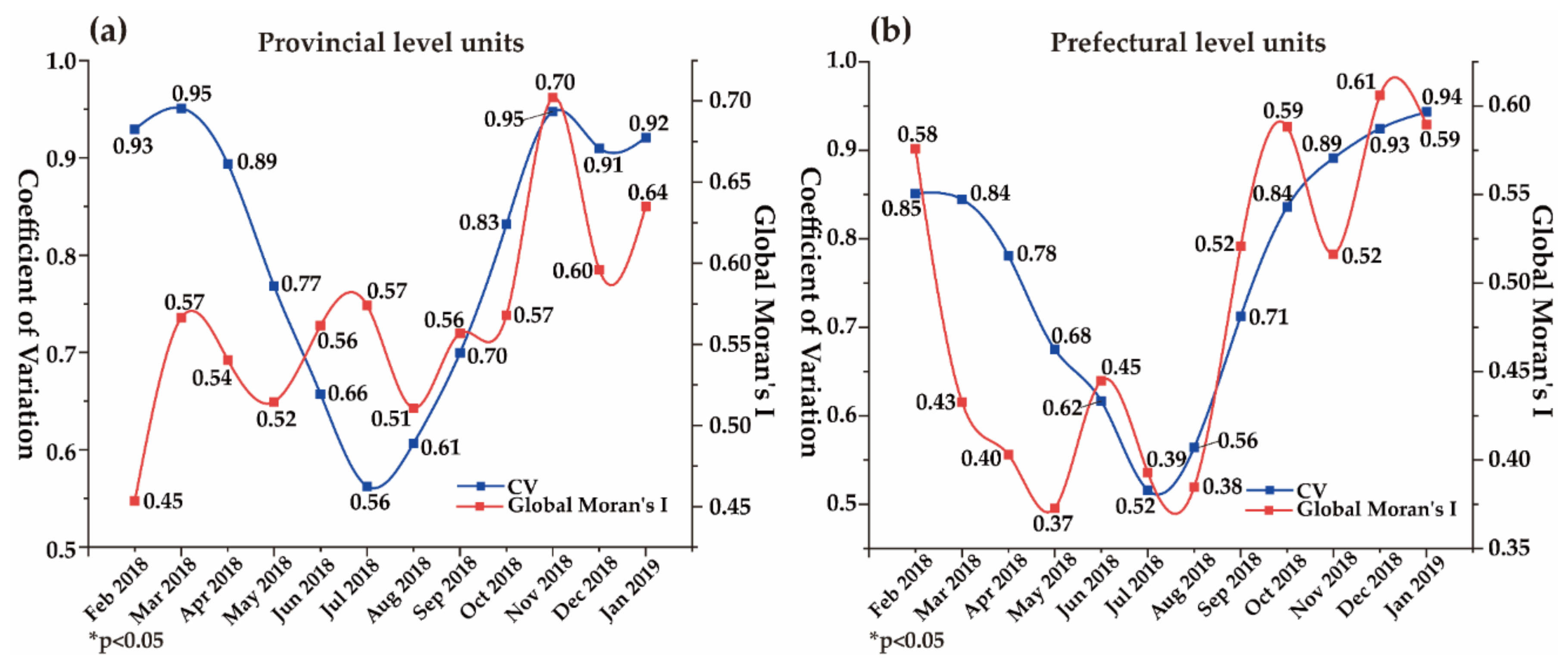
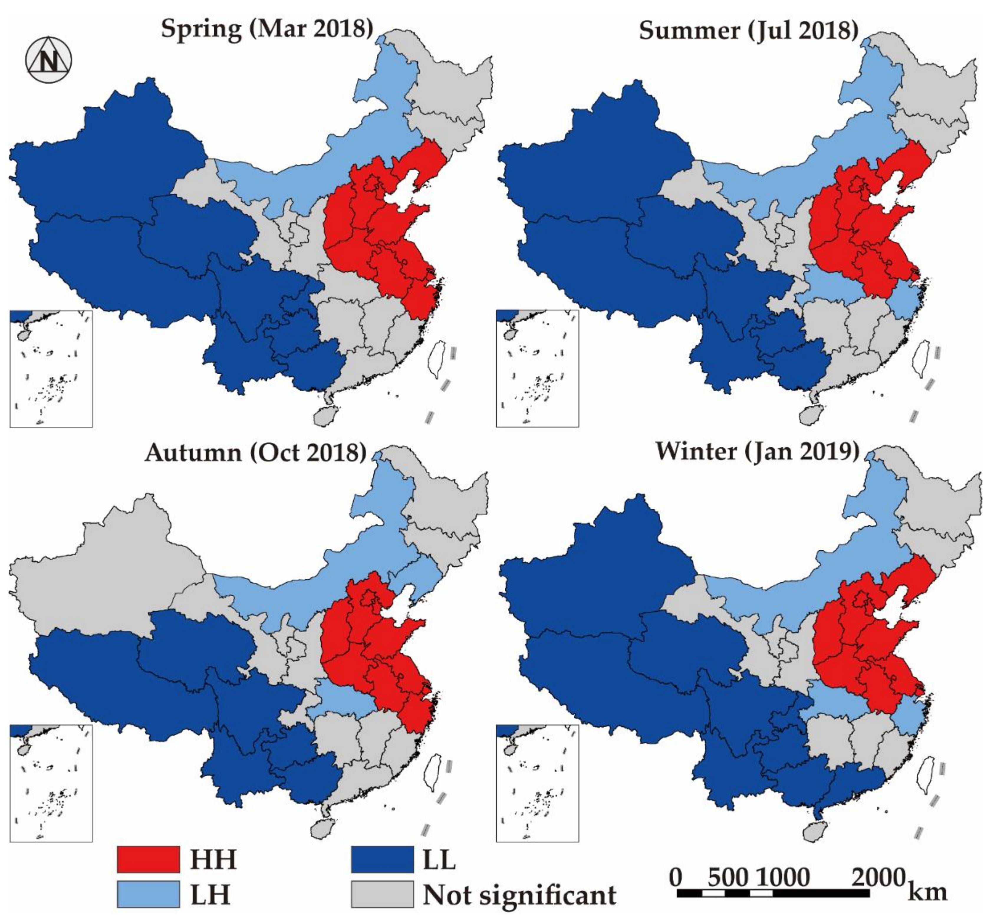
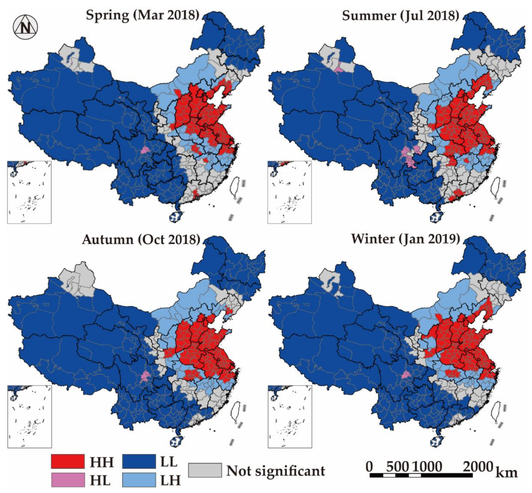
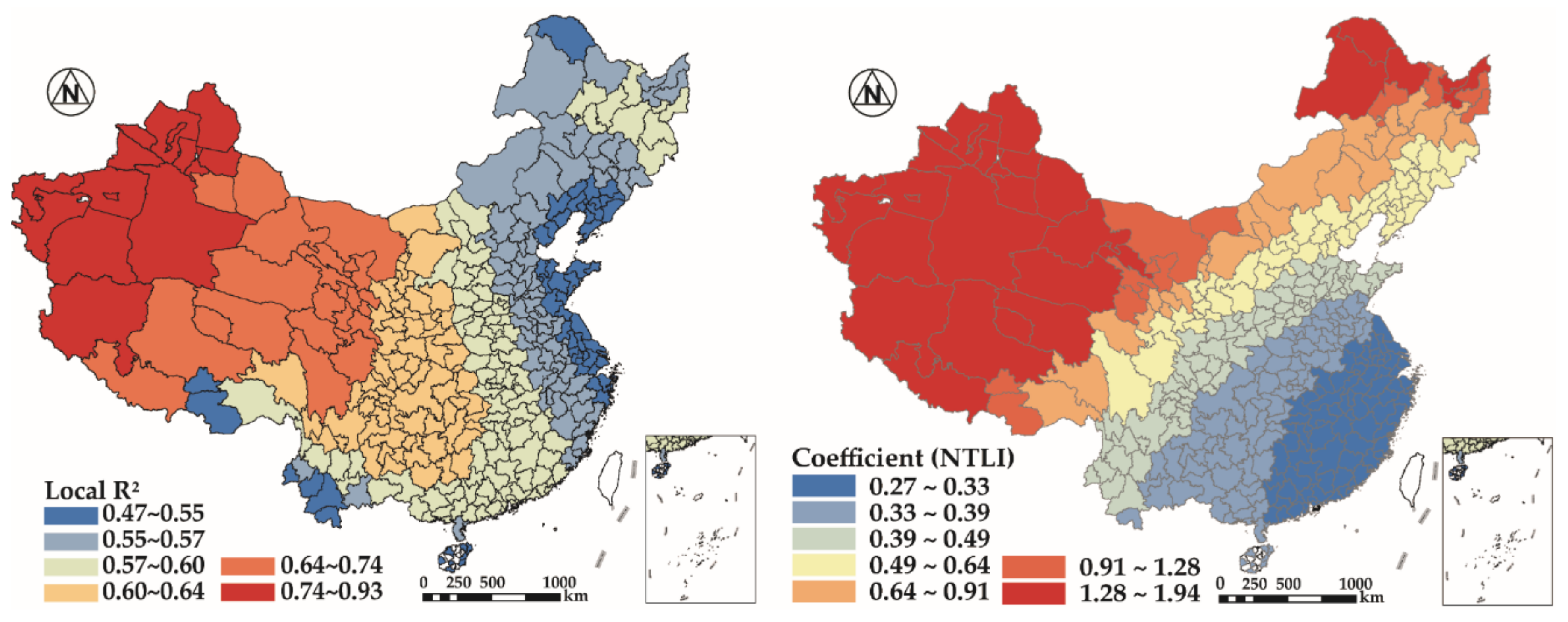
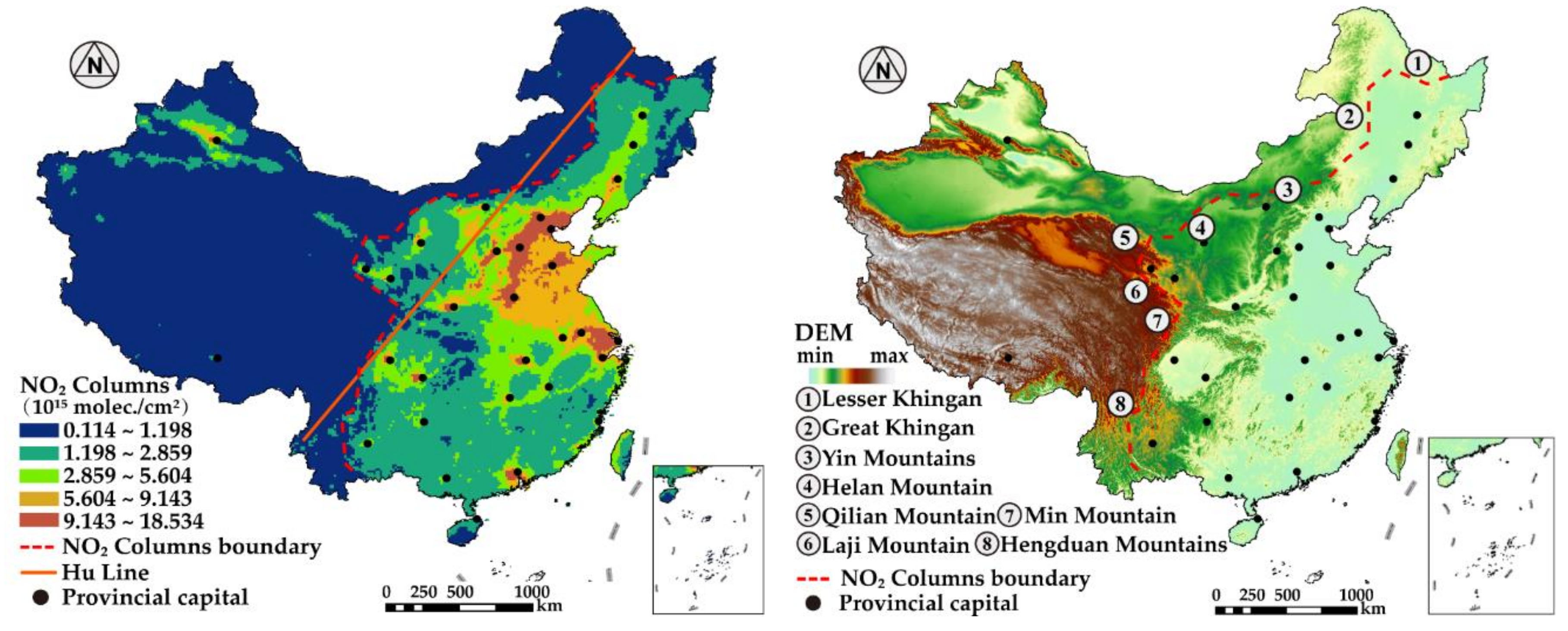
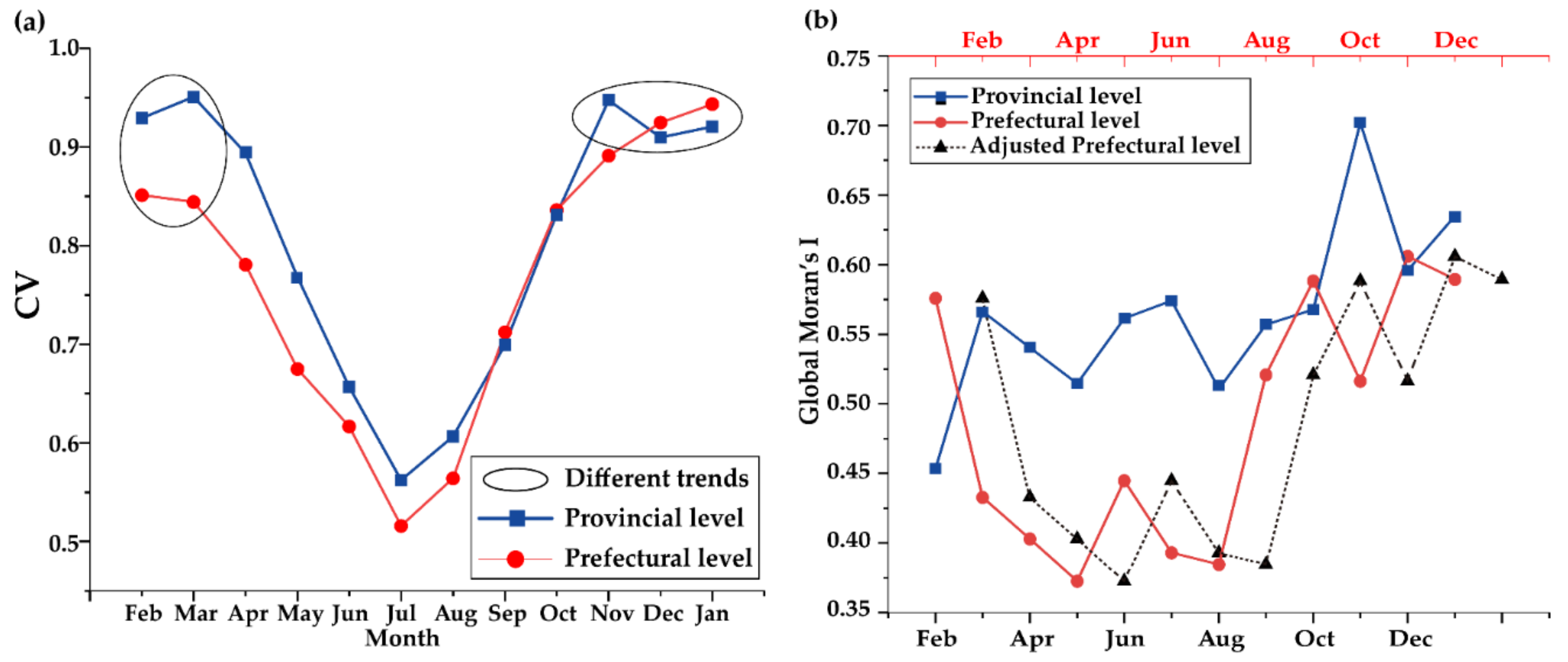
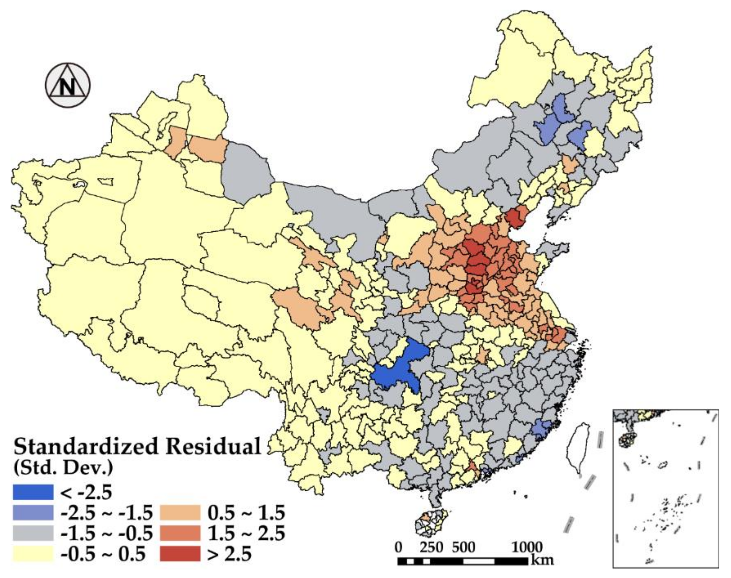
Table 1.
The monthly statistic results of tropospheric NO2 column concentration and temperature (°C).
Table 1.
The monthly statistic results of tropospheric NO2 column concentration and temperature (°C).
| Year | 2018 | 2019 | ||||||||||
|---|---|---|---|---|---|---|---|---|---|---|---|---|
| Month | Feb | Mar | Apr | May | Jun | Jul | Aug | Sep | Oct | Nov | Dec | Jan |
| Min | 0.01 | 0.01 | 0.01 | 0.01 | 0.03 | 0.01 | 0.02 | 0.01 | 0.01 | 0.01 | 0.01 | 0.01 |
| Max | 29.01 | 27.99 | 23.54 | 22.65 | 14.33 | 11.19 | 15.86 | 16.01 | 37.96 | 38.41 | 34.40 | 41.52 |
| Mean | 1.90 | 1.84 | 1.68 | 1.52 | 1.45 | 1.35 | 1.35 | 1.47 | 1.94 | 2.24 | 2.60 | 2.61 |
| Std | 2.71 | 2.47 | 2.06 | 1.56 | 1.24 | 0.90 | 0.98 | 1.52 | 2.66 | 3.40 | 4.13 | 4.23 |
| Temperature | −2.0 | 7.0 | 12.3 | 17.0 | 20.7 | 22.9 | 21.9 | 16.7 | 9.8 | 3.1 | −3.8 | −4.1 |
Table 2.
Results of Spatial Lag Model at provincial unit.
| Impact Factor | Coefficient | Std.Error | z-Value | Probability |
|---|---|---|---|---|
| W_NO2 | 0.454 | 0.174 | 2.614 | 0.009 |
| CONSTANT | −12.337 | 5.668 | −2.176 | 0.030 |
| Nighttime light intensity | 0.451 | 0.128 | 3.527 | 0.000 |
| Digital Elevation Model (DEM) | −0.038 | 0.028 | −1.323 | 0.186 |
| Proportion of second industry | 0.146 | 0.064 | 2.275 | 0.023 |
| Proportion of third industry | 0.156 | 0.071 | 2.194 | 0.028 |
| R-squared | 0.781(0.722) | Log Likelihood | −54.212(−57.268) | |
| Akaike Info Criterion | 120.423(124.536) | Prob | 0.01342 | |
| Schwarz Criterion | 129.027(131.706) |
* Ordinary Least Square (OLS) indicators are list in parentheses.
Table 3.
The model indicator difference between Geographic Weighted Regression (GWR) and OLS at prefectural unit.
Table 3.
The model indicator difference between Geographic Weighted Regression (GWR) and OLS at prefectural unit.
| Model | GWR | OLS | |
|---|---|---|---|
| Model indicator | R2 | 0.643 | 0.505 |
| Adj.R2 | 0.620 | 0.497 | |
| Akaike Info Criterion corrected (AICc) | 1395 | 1488 | |
| Sigma-Squared | 3.040 | 4.025 | |
| Sigma-square Maximum Likelihood (Sigma-square ML) | 2.855 | 3.956 | |
| P-value | 0.000 | 0.000 | |
© 2019 by the authors. Licensee MDPI, Basel, Switzerland. This article is an open access article distributed under the terms and conditions of the Creative Commons Attribution (CC BY) license (http://creativecommons.org/licenses/by/4.0/).
Share and Cite
MDPI and ACS Style
Zheng, Z.; Yang, Z.; Wu, Z.; Marinello, F. Spatial Variation of NO2 and Its Impact Factors in China: An Application of Sentinel-5P Products. Remote Sens. 2019, 11, 1939. https://0-doi-org.brum.beds.ac.uk/10.3390/rs11161939
AMA Style
Zheng Z, Yang Z, Wu Z, Marinello F. Spatial Variation of NO2 and Its Impact Factors in China: An Application of Sentinel-5P Products. Remote Sensing. 2019; 11(16):1939. https://0-doi-org.brum.beds.ac.uk/10.3390/rs11161939
Chicago/Turabian StyleZheng, Zihao, Zhiwei Yang, Zhifeng Wu, and Francesco Marinello. 2019. "Spatial Variation of NO2 and Its Impact Factors in China: An Application of Sentinel-5P Products" Remote Sensing 11, no. 16: 1939. https://0-doi-org.brum.beds.ac.uk/10.3390/rs11161939
Note that from the first issue of 2016, this journal uses article numbers instead of page numbers. See further details here.