Assimilation of Remotely-Sensed LAI into WOFOST Model with the SUBPLEX Algorithm for Improving the Field-Scale Jujube Yield Forecasts

 ,
,
Abstract
:
1. Introduction
- (1)
- To develop SUBPLEX algorithm to optimize the key input parameters of the WFOST model for reducing the uncertainty.
- (2)
- To compare the yield prediction performance of the proposed SUBPLEX assimilation with the EnKF method.
2. Materials and Methods
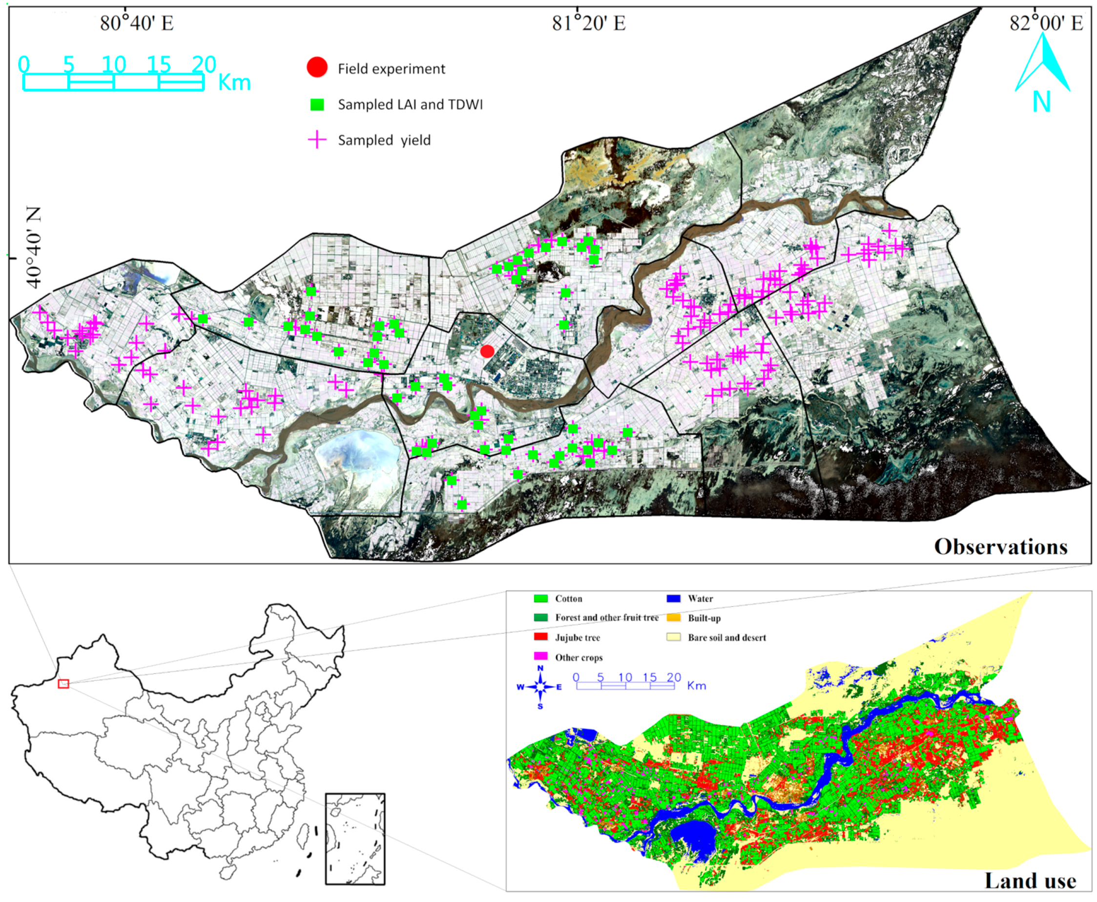
2.1. Study Region
2.2. Model and Data
2.2.1. WOFOST Model
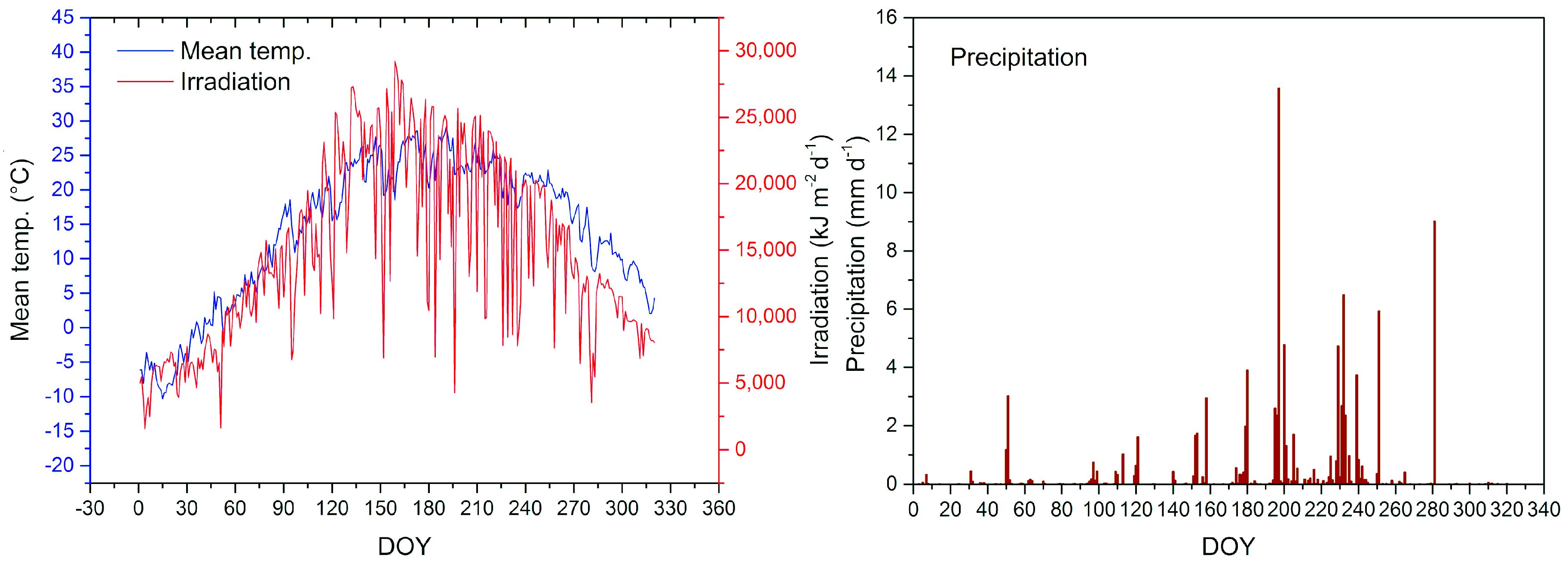
2.2.2. Study Data
2.3. Remotely Sensed LAI
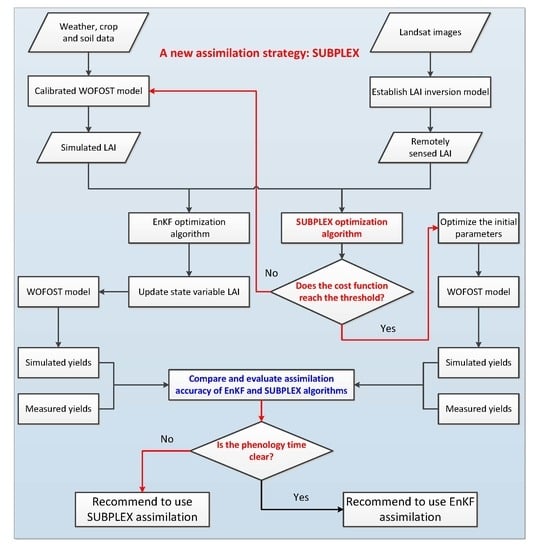
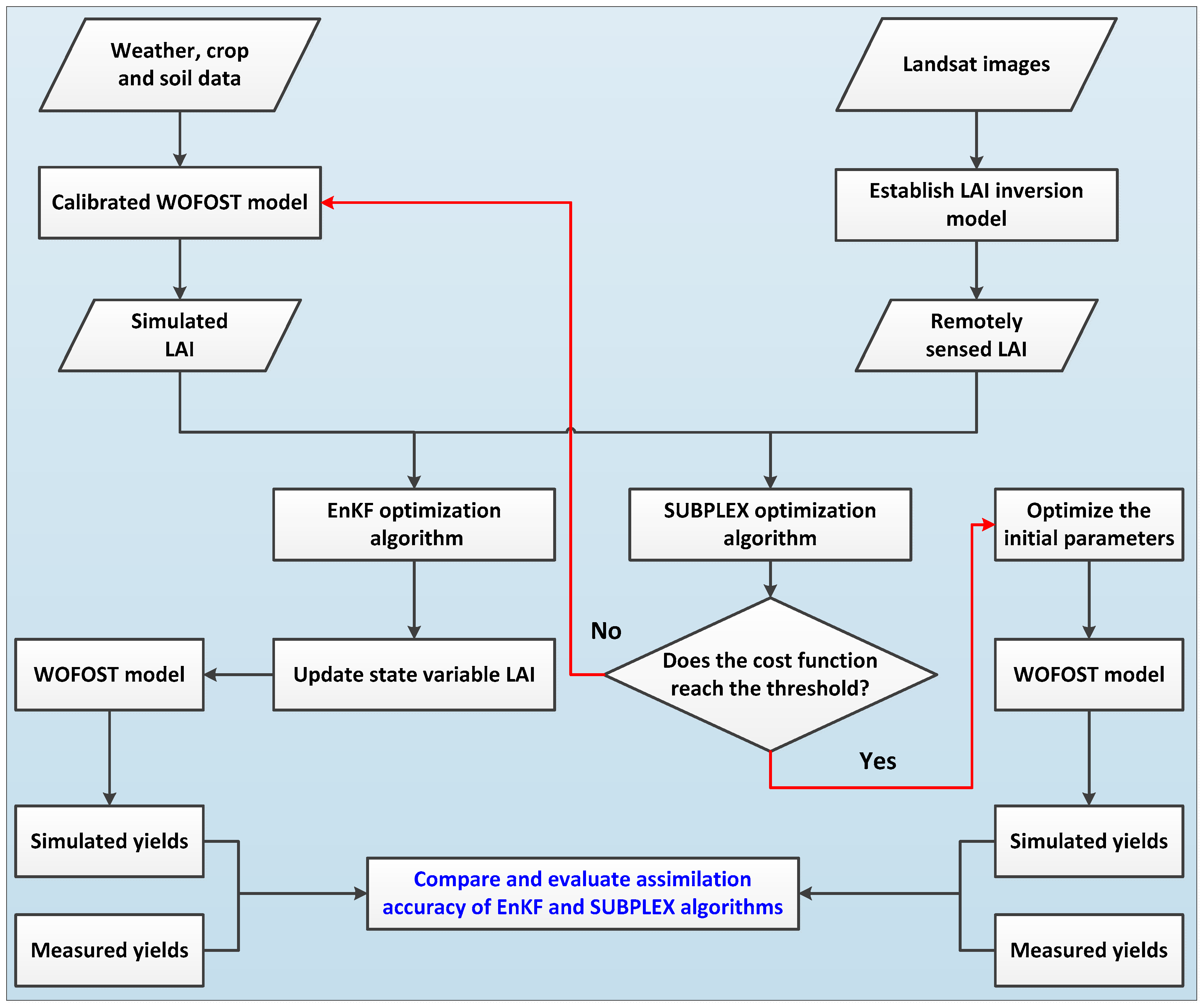
2.4. Assimilation Strategy
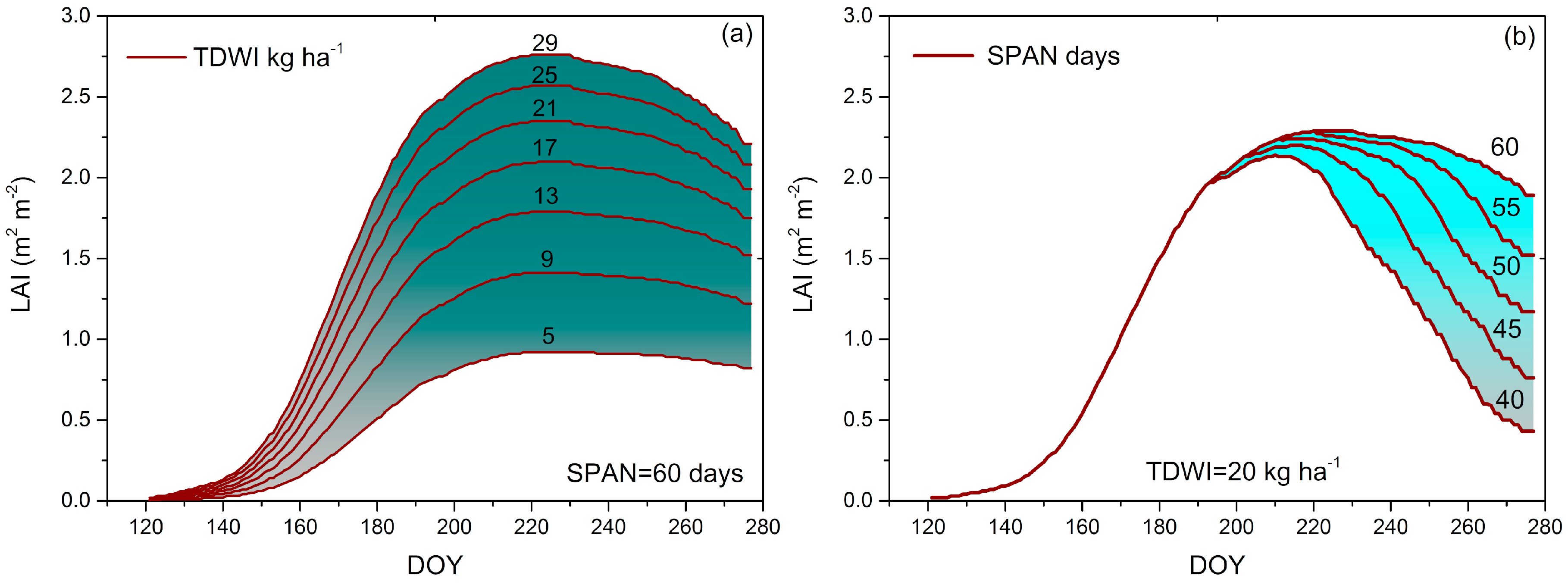
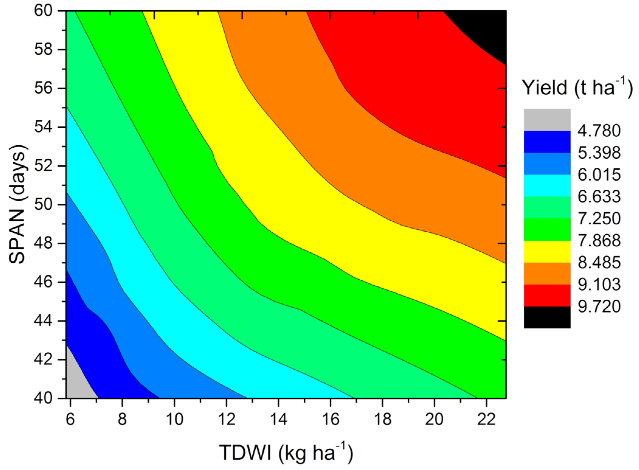
2.4.1. Selection of Reinitialized Parameters for WOFOST
2.4.2. Assimilation Methods
3. Results
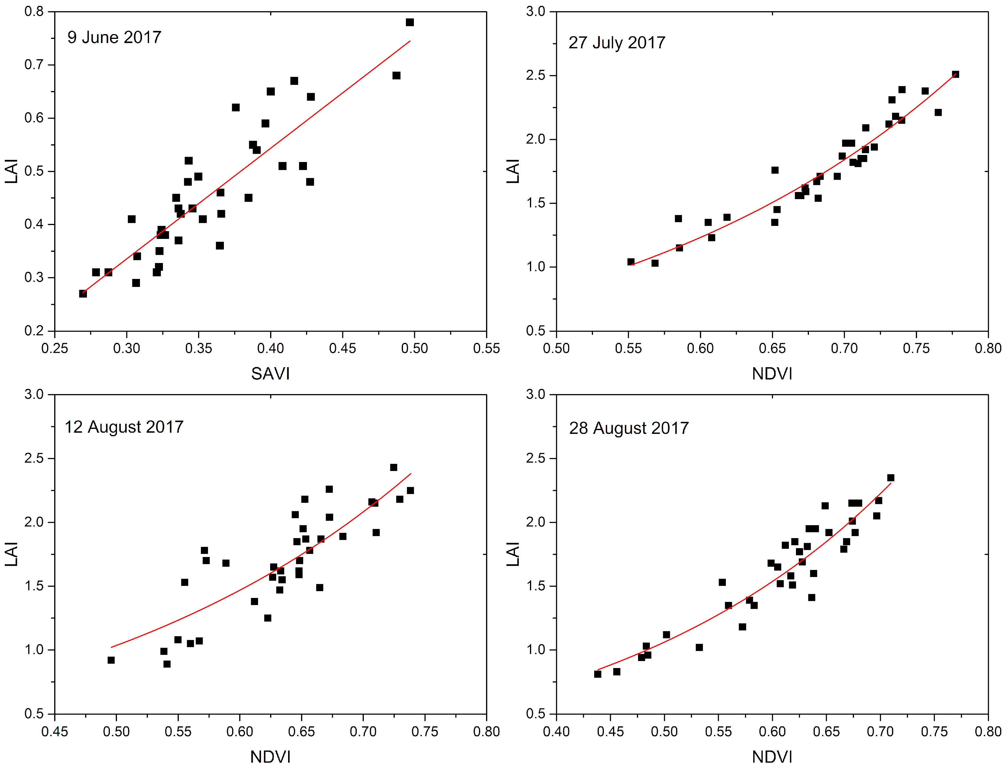
3.1. Remotely Sensed LAI
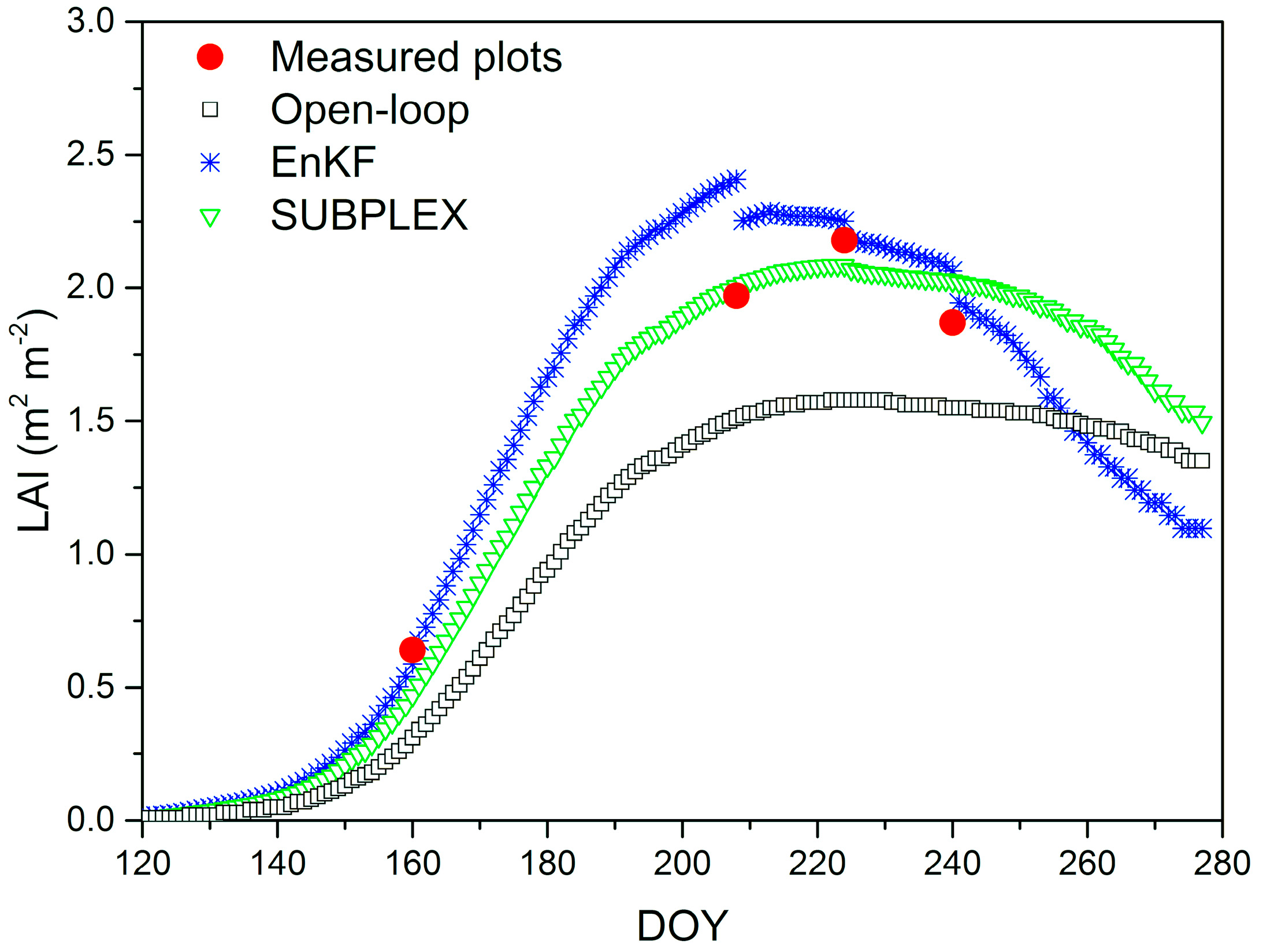
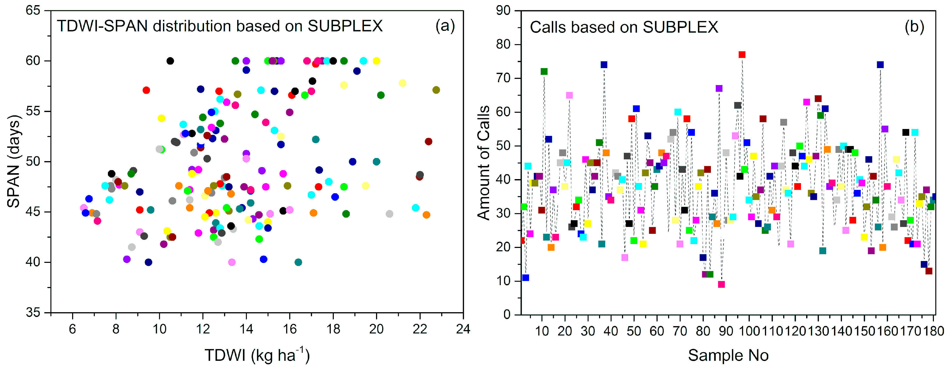
3.2. Assimilation Process
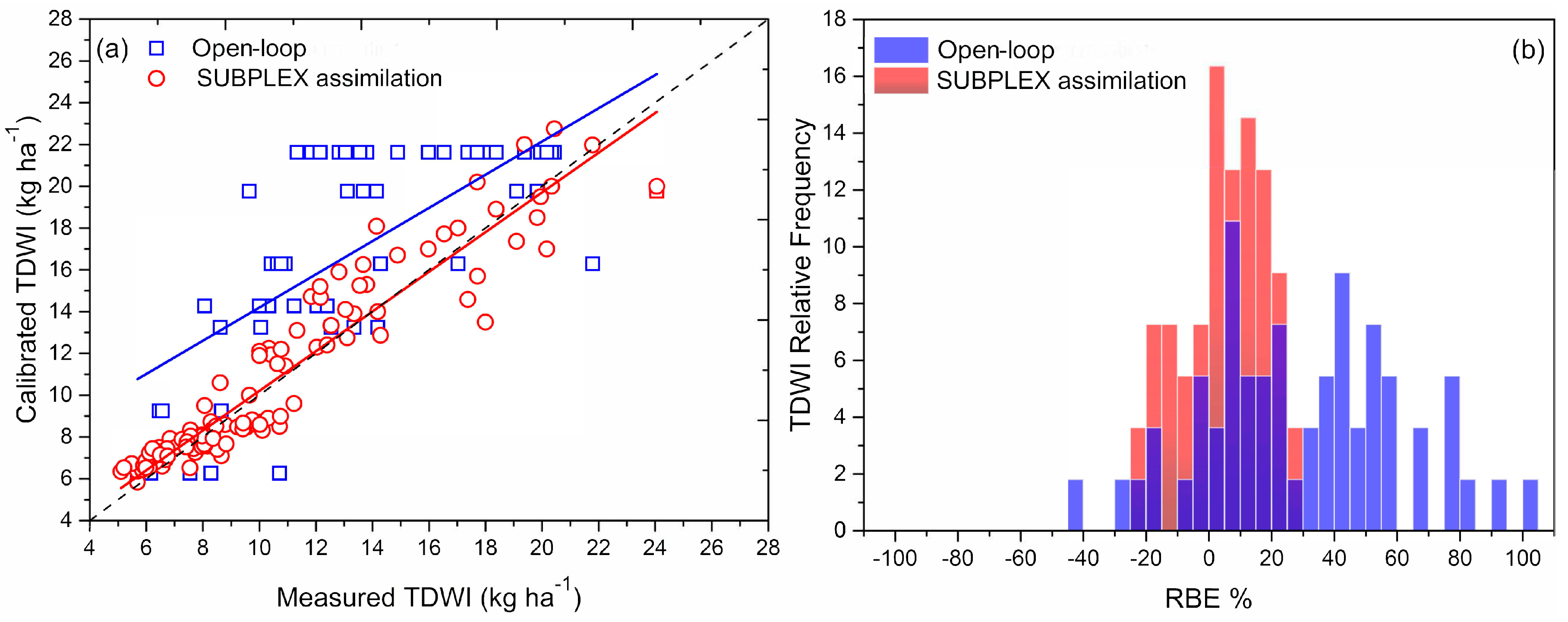
3.3. SUBPLEX Assimilation Evaluation Based on the Field-Measured LAI
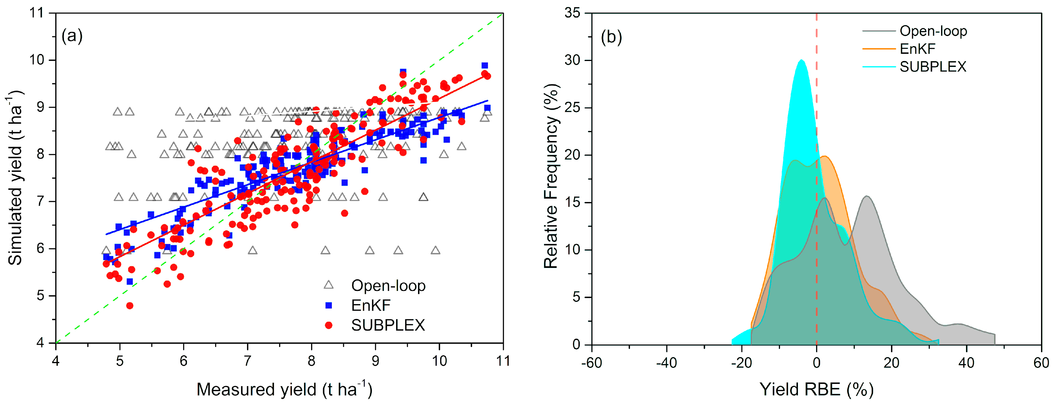
3.4. Evaluation of Model Performance Based on Remotely Sensed LAI
4. Discussion
5. Conclusions
Author Contributions
Funding
Acknowledgments
Conflicts of Interest
References
- Gao, Q.; Wu, C.; Wang, M. The Jujube (Ziziphus Jujuba Mill.) Fruit: A review of current knowledge of fruit composition and health benefits. J. Agric. Food Chem. 2013, 61, 3351–3363. [Google Scholar] [CrossRef] [PubMed]
- Li, J.W.; Fan, L.P.; Ding, S.D.; Ding, X.L. Nutritional composition of five cultivars of chinese jujube. Food Chem. 2007, 103, 454–460. [Google Scholar] [CrossRef]
- Jin, X.; Kumar, L.; Li, Z.; Feng, H.; Xu, X.; Yang, G.; Wang, J. A review of data assimilation of remote sensing and crop models. Eur. J. Agron. 2018, 92, 141–152. [Google Scholar] [CrossRef]
- Zhou, G.; Liu, X.; Liu, M. Assimilating Remote Sensing Phenological Information into the WOFOST Model for Rice Growth Simulation. Remote Sens. 2019, 11, 268. [Google Scholar] [CrossRef]
- Nearing, G.S.; Crow, W.T.; Thorp, K.R.; Moran, M.S.; Reichle, R.H.; Gupta, H.V. Assimilating remote sensing observations of leaf area index and soil moisture for wheat yield estimates: An observing system simulation experiment. Water Resour. Res. 2012, 48, W05525. [Google Scholar] [CrossRef]
- Fang, H.; Liang, S.; Hoogenboom, G.; Teasdale, J.; Cavigelli, M. Corn-yield estimation through assimilation of remotely sensed data into the CSM-CERES-Maize model. Int. J. Remote Sens. 2008, 29, 3011–3032. [Google Scholar] [CrossRef]
- Huang, J.; Ma, H.; Su, W.; Zhang, X.; Huang, Y.; Fan, J.; Wu, W. Jointly Assimilating MODIS LAI and et Products into the SWAP Model for Winter Wheat Yield Estimation. IEEE J. Sel. Top. Appl. Earth Obs. Remote Sens. 2015, 8, 4060–4071. [Google Scholar] [CrossRef]
- Huang, J.; Sedano, F.; Huang, Y.; Ma, H.; Li, X.; Liang, S.; Tian, L.; Zhang, X.; Fan, J.; Wu, W. Assimilating a synthetic Kalman filter leaf area index series into the WOFOST model to improve regional winter wheat yield estimation. Agric. For. Meteorol. 2016, 216, 188–202. [Google Scholar] [CrossRef]
- Huang, J.; Tian, L.; Liang, S.; Ma, H.; Becker-Reshef, I.; Huang, Y.; Su, W.; Zhang, X.; Zhu, D.; Wu, W. Improving winter wheat yield estimation by assimilation of the leaf area index from Landsat TM and MODIS data into the WOFOST model. Agric. For. Meteorol. 2015, 204, 106–121. [Google Scholar] [CrossRef] [Green Version]
- Yao, F.; Tang, Y.; Wang, P.; Zhang, J. Estimation of maize yield by using a process-based model and remote sensing data in the Northeast China Plain. Phys. Chem. Earth 2015, 87, 142–152. [Google Scholar] [CrossRef]
- Jin, X.; Yang, G.; Xu, X.; Yang, H.; Feng, H.; Li, Z.; Shen, J.; Zhao, C.; Lan, Y. Combined multi-temporal optical and radar parameters for estimating LAI and biomass in winter wheat using HJ and RADARSAR-2 data. Remote Sens. 2015, 7, 13251–13272. [Google Scholar] [CrossRef]
- Wang, J.; Li, X.; Lu, L.; Fang, F. Estimating near future regional corn yields by integrating multi-source observations into a crop growth model. Eur. J. Agron. 2013, 49, 126–140. [Google Scholar] [CrossRef]
- Chakrabarti, S.; Bongiovanni, T.; Judge, J.; Zotarelli, L.; Bayer, C. Assimilation of SMOS soil moisture for quantifying drought impacts on crop yield in agricultural regions. IEEE J. Sel. Top. Appl. Earth Obs. Remote Sens. 2014, 7, 3867–3879. [Google Scholar] [CrossRef]
- Ines, A.V.M.; Das, N.N.; Hansen, J.W.; Njoku, E.G. Assimilation of remotely sensed soil moisture and vegetation with a crop simulation model for maize yield prediction. Remote Sens. Environ. 2013, 138, 149–164. [Google Scholar] [CrossRef] [Green Version]
- Mishra, A.K.; Ines, A.V.M.; Das, N.N.; Prakash Khedun, C.; Singh, V.P.; Sivakumar, B.; Hansen, J.W. Anatomy of a local-scale drought: Application of assimilated remote sensing products, crop model, and statistical methods to an agricultural drought study. J. Hydrol. 2015, 526, 15–29. [Google Scholar] [CrossRef]
- Zhuo, W.; Huang, J.; Li, L.; Zhang, X.; Ma, H.; Gao, X.; Huang, H.; Xu, B.; Xiao, X. Assimilating Soil Moisture Retrieved from Sentinel-1 and Sentinel-2 Data into WOFOST Model to Improve Winter Wheat Yield Estimation. Remote Sens. 2019, 11, 1618. [Google Scholar] [CrossRef]
- Huang, J.; Ma, H.; Sedano, F.; Lewis, P.; Liang, S.; Wu, Q.; Su, W.; Zhang, X.; Zhu, D. Evaluation of regional estimates of winter wheat yield by assimilating three remotely sensed reflectance datasets into the coupled WOFOST–PROSAIL model. Eur. J. Agron. 2019, 102, 1–13. [Google Scholar] [CrossRef]
- Dong, T.; Liu, J.; Qian, B.; Zhao, T.; Jing, Q.; Geng, X.; Wang, J.; Huffman, T.; Shang, J. Estimating winter wheat biomass by assimilating leaf area index derived from fusion of Landsat-8 and MODIS data. Int. J. Appl. Earth Obs. Geoinf. 2016, 49, 63–74. [Google Scholar] [CrossRef]
- Ma, G.; Huang, J.; Wu, W.; Fan, J.; Zou, J.; Wu, S. Assimilation of MODIS-LAI into the WOFOST model for forecasting regional winter wheat yield. Math. Comput. Model. 2013, 58, 634–643. [Google Scholar] [CrossRef]
- Ren, J.; Liu, X.; Chen, Z.; Tang, H. Extracting spatial information of harvest index for winter wheat based on modis NDVI in North China. In Proceedings of the International Geoscience and Remote Sensing Symposium (IGARSS), Honolulu, HI, USA, 25–30 July 2010; pp. 2143–2146. [Google Scholar]
- Dong, Y.; Wang, J.; Li, C.; Yang, G.; Wang, Q.; Liu, F.; Zhao, J.; Wang, H.; Huang, W. Comparison and analysis of data assimilation algorithms for predicting the leaf area index of crop canopies. IEEE J. Sel. Top. Appl. Earth Obs. Remote Sens. 2013, 6, 188–201. [Google Scholar] [CrossRef]
- Dong, Y.; Zhao, C.; Yang, G.; Chen, L.; Wang, J.; Feng, H. Integrating a very fast simulated annealing optimization algorithm for crop leaf area index variational assimilation. Math. Comput. Model. 2013, 58, 877–885. [Google Scholar] [CrossRef]
- He, B.; Li, X.; Quan, X.; Qiu, S. Estimating the aboveground dry biomass of grass by assimilation of retrieved LAI into a crop growth model. IEEE J. Sel. Top. Appl. Earth Obs. Remote Sens. 2015, 8, 550–561. [Google Scholar] [CrossRef]
- Jin, H.; Li, A.; Wang, J.; Bo, Y. Improvement of spatially and temporally continuous crop leaf area index by integration of CERES-Maize model and MODIS data. Eur. J. Agron. 2016, 78, 1–12. [Google Scholar] [CrossRef]
- Guo, C.; Zhang, L.; Zhou, X.; Zhu, Y.; Cao, W.; Qiu, X.; Cheng, T.; Tian, Y. Integrating remote sensing information with crop model to monitor wheat growth and yield based on simulation zone partitioning. Precis. Agric. 2017, 19, 55–78. [Google Scholar] [CrossRef]
- Jin, X.; Li, Z.; Yang, G.; Yang, H.; Feng, H.; Xu, X.; Wang, J.; Li, X.; Luo, J. Winter wheat yield estimation based on multi-source medium resolution optical and radar imaging data and the AquaCrop model using the particle swarm optimization algorithm. ISPRS J. Photogramm. Remote Sens. 2017, 126, 24–37. [Google Scholar] [CrossRef]
- Li, Z.; Wang, J.; Xu, X.; Zhao, C.; Jin, X.; Yang, G.; Feng, H. Assimilation of two variables derived from hyperspectral data into the DSSAT-CERES model for grain yield and quality estimation. Remote Sens. 2015, 7, 12400–12418. [Google Scholar] [CrossRef]
- Jin, M.; Liu, X.; Wu, L.; Liu, M. An improved assimilation method with stress factors incorporated in the WOFOST model for the efficient assessment of heavy metal stress levels in rice. Int. J. Appl. Earth Obs. Geoinf. 2015, 41, 118–129. [Google Scholar] [CrossRef]
- Liu, F.; Liu, X.; Ding, C.; Wu, L. The dynamic simulation of rice growth parameters under cadmium stress with the assimilation of multi-period spectral indices and crop model. Field Crops Res. 2015, 183, 225–234. [Google Scholar] [CrossRef]
- Silvestro, P.C.; Pignatti, S.; Pascucci, S.; Yang, H.; Li, Z.; Yang, G.; Huang, W.; Casa, R. Estimating wheat yield in China at the field and district scale from the assimilation of satellite data into the Aquacrop and simple algorithm for yield (SAFY) models. Remote Sens. 2017, 9, 509. [Google Scholar] [CrossRef]
- Fang, H.; Liang, S.; Hoogenboom, G. Integration of MODIS LAI and vegetation index products with the CSM-CERES-Maize model for corn yield estimation. Int. J. Remote Sens. 2011, 32, 1039–1065. [Google Scholar] [CrossRef]
- Tian, L.; Li, Z.; Huang, J.; Wang, L.; Su, W.; Zhang, C.; Liu, J. Comparison of Two Optimization Algorithms for Estimating Regional Winter Wheat Yield by Integrating MODIS Leaf Area Index and World Food Studies Model. Sens. Lett. 2013, 11, 1261–1268. [Google Scholar] [CrossRef]
- Claverie, M.; Demarez, V.; Duchemin, B.; Hagolle, O.; Keravec, P.; Marciel, B.; Ceschia, E.; Dejoux, J.F.; Dedieu, G. Spatialization of crop leaf area index and biomass by combining a simple crop model safy and high spatial and temporal resolutions remote sensing data. In Proceedings of the International Geoscience and Remote Sensing Symposium (IGARSS), Cape Town, South Africa, 12–17 July 2009; Volume 3. [Google Scholar]
- Jégo, G.; Pattey, E.; Liu, J. Using Leaf Area Index, retrieved from optical imagery, in the STICS crop model for predicting yield and biomass of field crops. Field Crops Res. 2012, 131, 63–74. [Google Scholar] [CrossRef]
- Dente, L.; Satalino, G.; Mattia, F.; Rinaldi, M. Assimilation of leaf area index derived from ASAR and MERIS data into CERES-Wheat model to map wheat yield. Remote Sens. Environ. 2008, 112, 1395–1407. [Google Scholar] [CrossRef]
- Hu, S.; Mo, X.; Lin, Z. Optimizing the photosynthetic parameter Vcmax by assimilating MODIS-fPAR and MODIS-NDVI with a process-based ecosystem model. Agric. For. Meteorol. 2014, 198, 320–334. [Google Scholar] [CrossRef]
- Morel, J.; Todoroff, P.; Bégué, A.; Bury, A.; Martiné, J.F.; Petit, M. Toward a satellite-based system of sugarcane yield estimation and forecasting in smallholder farming conditions: A case study on reunion island. Remote Sens. 2014, 6, 6620–6635. [Google Scholar] [CrossRef]
- Ines, A.V.M.; Honda, K.; Das Gupta, A.; Droogers, P.; Clemente, R.S. Combining remote sensing-simulation modeling and genetic algorithm optimization to explore water management options in irrigated agriculture. Agric. Water Manag. 2006, 83, 221–232. [Google Scholar] [CrossRef] [Green Version]
- Wang, H.; Zhu, Y.; Li, W.; Cao, W.; Tian, Y. Integrating remotely sensed leaf area index and leaf nitrogen accumulation with RiceGrow model based on particle swarm optimization algorithm for rice grain yield assessment. J. Appl. Remote Sens. 2014, 8, 083674. [Google Scholar] [CrossRef] [Green Version]
- Zhu, X.; Zhao, Y.; Feng, X. A methodology for estimating Leaf Area Index by assimilating remote sensing data into crop model based on temporal and spatial knowledge. Chin. Geogr. Sci. 2013, 23, 550–561. [Google Scholar] [CrossRef]
- Zhao, Y.; Chen, S.; Shen, S. Assimilating remote sensing information with crop model using Ensemble Kalman Filter for improving LAI monitoring and yield estimation. Ecol. Model. 2013, 270, 30–42. [Google Scholar] [CrossRef]
- Xie, Y.; Wang, P.; Bai, X.; Khan, J.; Zhang, S.; Li, L.; Wang, L. Assimilation of the leaf area index and vegetation temperature condition index for winter wheat yield estimation using Landsat imagery and the CERES-Wheat model. Agric. For. Meteorol. 2017, 246, 194–206. [Google Scholar] [CrossRef]
- Wu, S.; Huang, J.; Liu, X.; Fan, J.; Ma, G.; Zou, J. Assimilating MODIS-LAI into crop growth model with EnKF to predict regional crop yield. In IFIP Advances in Information and Communication Technology, Proceedings of the IFIP Advances in Information and Communication Technology, Beijing, China, 29–31 October 2011; Springer: Berlin/Heidelberg, Germany, 2012; Volume 370, pp. 410–418. [Google Scholar]
- Pauwels, V.R.N.; Verhoest, N.E.C.; De Lannoy, G.J.M.; Guissard, V.; Lucau, C.; Defourny, P. Optimization of a coupled hydrology-crop growth model through the assimilation of observed soil moisture and leaf area index values using an ensemble Kalman filter. Water Resour. Res. 2007, 43, W04421. [Google Scholar] [CrossRef]
- Ma, H.; Huang, J.; Zhu, D.; Liu, J.; Su, W.; Zhang, C.; Fan, J. Estimating regional winter wheat yield by assimilation of time series of HJ-1 CCD NDVI into WOFOST-ACRM model with Ensemble Kalman Filter. Math. Comput. Model. 2013, 58, 759–770. [Google Scholar] [CrossRef]
- Li, Y.; Zhou, Q.; Zhou, J.; Zhang, G.; Chen, C.; Wang, J. Assimilating remote sensing information into a coupled hydrology-crop growth model to estimate regional maize yield in arid regions. Ecol. Model. 2014, 291, 15–27. [Google Scholar] [CrossRef]
- De Wit, A.J.W.; van Diepen, C.A. Crop model data assimilation with the Ensemble Kalman filter for improving regional crop yield forecasts. Agric. For. Meteorol. 2007, 146, 38–56. [Google Scholar] [CrossRef]
- Curnel, Y.; de Wit, A.J.W.; Duveiller, G.; Defourny, P. Potential performances of remotely sensed LAI assimilation in WOFOST model based on an OSS Experiment. Agric. For. Meteorol. 2011, 151, 1843–1855. [Google Scholar] [CrossRef]
- Cheng, Z.; Meng, J.; Qiao, Y.; Wang, Y.; Dong, W.; Han, Y. Preliminary study of soil available nutrient simulation using a modified WOFOST model and time-series remote sensing observations. Remote Sens. 2018, 10, 64. [Google Scholar] [CrossRef]
- Bolten, J.D.; Crow, W.T.; Jackson, T.J.; Zhan, X.; Reynolds, C.A. Evaluating the Utility of Remotely Sensed Soil Moisture Retrievals for Operational Agricultural Drought Monitoring. IEEE J. Sel. Top. Appl. Earth Obs. Remote Sens. 2010, 3, 57–66. [Google Scholar] [CrossRef]
- Jiang, Z.; Chen, Z.; Chen, J.; Liu, J.; Ren, J.; Li, Z.; Sun, L.; Li, H. Application of crop model data assimilation with a particle filter for estimating regional winter wheat yields. IEEE J. Sel. Top. Appl. Earth Obs. Remote Sens. 2014, 7, 4422–4431. [Google Scholar] [CrossRef]
- Vazifedoust, M.; van Dam, J.C.; Bastiaanssen, W.G.M.; Feddes, R.A. Assimilation of satellite data into agrohydrological models to improve crop yield forecasts. Int. J. Remote Sens. 2009, 30, 2523–2545. [Google Scholar] [CrossRef]
- Chen, Y.; Zhang, Z.; Tao, F. Improving regional winter wheat yield estimation through assimilation of phenology and leaf area index from remote sensing data. Eur. J. Agron. 2018, 101, 163–173. [Google Scholar] [CrossRef]
- Huang, Y.; Zhu, Y.; Li, W.; Cao, W.; Tian, Y. Assimilating Remotely Sensed Information with the WheatGrow Model Based on the Ensemble Square Root Filter forImproving Regional Wheat Yield Forecasts. Plant Prod. Sci. 2013, 16, 352–364. [Google Scholar] [CrossRef]
- Huang, J.; Gómez-Dans, J.; Huang, H.; Ma, H.; Wu, Q.; Lewis, P.; Liang, S.; Chen, Z.; Xue, J.; Wu, Y.; et al. Assimilation of remote sensing into crop growth models: current status and perspectives. Agric. For. Meteorol. 2019, 276–277, 107609. [Google Scholar] [CrossRef]
- Rowan, T.H. Functional Stability Analysis of Numerical Algorithms. Ph.D. Thesis, University of Texas, Austin, TX, USA, 1990. [Google Scholar]
- Jonsén, P.; Isaksson, E.; Sundin, K.G.; Oldenburg, M. Identification of lumped parameter automotive crash models for bumper system development. Int. J. Crashworthiness 2009, 14, 533–541. [Google Scholar] [CrossRef]
- De Wit, A.; Boogaard, H.; Fumagalli, D.; Janssen, S.; Knapen, R.; van Kraalingen, D.; Supit, I.; van der Wijngaart, R.; van Diepen, K. 25 years of the WOFOST cropping systems model. Agric. Syst. 2019, 168, 154–167. [Google Scholar] [CrossRef]
- Bai, T.; Zhang, N.; Mercatoris, B.; Chen, Y. Improving Jujube Fruit Tree Yield Estimation at the Field Scale by Assimilating a Single Landsat Remotely-Sensed LAI into the WOFOST Model. Remote Sens. 2019, 11, 1119. [Google Scholar] [CrossRef]
- De Wit, A.; Duveiller, G.; Defourny, P. Estimating regional winter wheat yield with WOFOST through the assimilation of green area index retrieved from MODIS observations. Agric. For. Meteorol. 2012, 164, 39–52. [Google Scholar] [CrossRef]
- Van Diepen, C.A.; Wolf, J.; van Keulen, H.; Rappoldt, C. WOFOST: A simulation model of crop production. Soil Use Manag. 1989, 5, 16–24. [Google Scholar] [CrossRef]
- Bai, T.; Zhang, N.; Mercatoris, B.; Chen, Y. Jujube yield prediction method combining Landsat 8 Vegetation Index and the phenological length. Comput. Electron. Agric. 2019, 162, 1011–1027. [Google Scholar] [CrossRef]
- Huete, A.R. A soil-adjusted vegetation index (SAVI). Remote Sens. Environ. 1988, 25, 295–309. [Google Scholar] [CrossRef]
- Pettorelli, N. The Normalized Difference Vegetation Index; Oxford University Press: London, UK, 2013; pp. 1–208. [Google Scholar] [CrossRef]


| Samples | Sampled Date | Max | Min | Average | STDEV.P |
|---|---|---|---|---|---|
| Yields of 181 samples | 1–15 November | 10.75 | 4.79 | 7.74 | 2.43 |
| TDWI of 55 samples | 25 April to 5 May | 24.06 | 5.69 | 13.45 | 7.53 |
| LAI of 55 samples | 9 June | 0.78 | 0.27 | 0.46 | 0.12 |
| 27 July | 2.51 | 1.03 | 1.76 | 0.37 | |
| 12 August | 2.43 | 0.89 | 1.70 | 0.40 | |
| 28 August | 2.35 | 0.81 | 1.62 | 0.41 |
| Name | Description | Set Value in This Study |
|---|---|---|
| the number of assimilated LAI | 4 | |
| function to be minimized | Equation (3) | |
| the number of optimized parameters for WOFOST | 2 (TDWI and SPAN) | |
| simplex reduction coefficient | 0.25 | |
| step reduction coefficient | 0.1 | |
| relative tolerance for convergence | 0.05 | |
| the range of TDWI | 5–30 | |
| the range of SPAN | 40–60 | |
| max-evaluation | maximum number of evaluations allowed | 200 |
| Initial step | the initial step size to compute numerical gradients | 0.5 for TDWI 1 for SPAN |
| Date | Calibrated R2 | Calibrated RMSE (%) m2 m−2 | Validated R2 | Validated RMSE (%) m2 m−2 |
|---|---|---|---|---|
| 09 June 2017 | 0.774 | 0.058 (12.7) | 0.770 | 0.061 (12.5) |
| 27 July 2017 | 0.918 | 0.108 (6.2) | 0.841 | 0.144 (8.1) |
| 12 August 2017 | 0.710 | 0.229 (13.6) | 0.779 | 0.180 (10.5) |
| 28 August 2017 | 0.884 | 0.115 (7.1) | 0.812 | 0.170 (10.4) |
| Mean t ha−1 | Maxmium t ha−1 | Minmium t ha−1 | R2 | RMSE (%) t ha−1 | |
|---|---|---|---|---|---|
| Field-measured yield at the 55 samples | 7.931 | 10.71 | 4.848 | – | – |
| Open-loop simulation | 8.271 | 8.89 | 5.946 | 0.58 | 0.95 (12.1) |
| EnKF assimilaiton | 7.717 | 9.887 | 5.303 | 0.81 | 0.65 (8.2) |
| SUBPLEX assimulaiton | 7.707 | 9.713 | 4.791 | 0.86 | 0.55 (7.0) |
| R2 | RMSE (%) ha−1 | MAE, % | Average RBE, % | |
|---|---|---|---|---|
| Open-loop simulation | 0.39 | 1.06 (13.8) | 12.5 | 8.65 |
| EnKF with remotely sensed LAI | 0.73 | 0.71 (9.2) | 7.73 | 0.77 |
| SUBPLEX with remotely sensed LAI | 0.78 | 0.64 (8.3) | 6.85 | −0.39 |
| Available Observations | R2 | RMSE (%) t ha−1 | MAE, % | Average RBE, % | |
|---|---|---|---|---|---|
| SUBPLEX | Four observations | 0.86 | 0.55 | 5.77 | −2.3 |
| Without 9 June | 0.84 | 0.59 | 6.04 | −1.75 | |
| Without 27 July | 0.85 | 0.58 | 6.01 | −1.48 | |
| Without 12 August | 0.81 | 0.65 | 6.35 | −3.31 | |
| Without 28 August (a) | 0.36 | 1.18 | 12.3 | 0.23 | |
| Without 28 August (b) | 0.73 | 0.77 | 9.02 | 4.49 | |
| EnKF | Four observations | 0.81 | 0.65 | 6.78 | −1.42 |
| Without 9 June | 0.65 | 0.88 | 8.78 | −7.69 | |
| Without 27 July | 0.75 | 0.75 | 7.93 | −1.87 | |
| Without 12 August | 0.74 | 0.76 | 7.98 | −1.59 | |
| Without 28 August | 0.71 | 0.81 | 8.73 | −1.02 |
© 2019 by the authors. Licensee MDPI, Basel, Switzerland. This article is an open access article distributed under the terms and conditions of the Creative Commons Attribution (CC BY) license (http://creativecommons.org/licenses/by/4.0/).
Share and Cite
Bai, T.; Wang, S.; Meng, W.; Zhang, N.; Wang, T.; Chen, Y.; Mercatoris, B. Assimilation of Remotely-Sensed LAI into WOFOST Model with the SUBPLEX Algorithm for Improving the Field-Scale Jujube Yield Forecasts. Remote Sens. 2019, 11, 1945. https://0-doi-org.brum.beds.ac.uk/10.3390/rs11161945
Bai T, Wang S, Meng W, Zhang N, Wang T, Chen Y, Mercatoris B. Assimilation of Remotely-Sensed LAI into WOFOST Model with the SUBPLEX Algorithm for Improving the Field-Scale Jujube Yield Forecasts. Remote Sensing. 2019; 11(16):1945. https://0-doi-org.brum.beds.ac.uk/10.3390/rs11161945
Chicago/Turabian StyleBai, Tiecheng, Shanggui Wang, Wenbo Meng, Nannan Zhang, Tao Wang, Youqi Chen, and Benoit Mercatoris. 2019. "Assimilation of Remotely-Sensed LAI into WOFOST Model with the SUBPLEX Algorithm for Improving the Field-Scale Jujube Yield Forecasts" Remote Sensing 11, no. 16: 1945. https://0-doi-org.brum.beds.ac.uk/10.3390/rs11161945